Fast parallel calculation of modified Bessel function
of the second kind and its derivatives

Abstract

There are three main types of numerical computations for the Bessel function of the second kind: series expansion, continued fraction, and asymptotic expansion. In addition, they are combined in the appropriate domain for each. However, there are some regions where the combination of these types requires sufficient computation time to achieve sufficient accuracy, however, efficiency is significantly reduced when parallelized. In the proposed method, we adopt a simple numerical integration concept of integral representation. We coarsely refine the integration range beforehand, and stabilize the computation time by performing the integration calculation at a fixed number of intervals. Experiments demonstrate that the proposed method can achieve the same level of accuracy as existing methods in less than half the computation time.

1 Introduction

The modified Bessel function of the second kind $K_{v}(x)$ is an important special function adopted in various fields [1]. In addition to mathematics and physics, it has become increasingly important in the fields of statistics and economics. For example, normal inverse Gaussian [2] has been garnering increasing attention in economics [3], biometrics [4, 5], and machine learning [6, 7].

Three numerical methods exist calculating the Bessel function $K_{v}$: series expansion–based [8], continued fraction-based [8, 9, 10, 11], and asymptotic expansion-based methods [12, 13]. Because each computation method exhibits different accuracies and computation time characteristics for $v$ and $x$, a combined implementation of these methods is generally adopted [14, 15, 16]. However, in some regions, an enormous amount of computation time is required for any method to achieve sufficient accuracy.

Recently, it has become common to adopt GPUs and multi-core processors to perform large-scale paralell or vectorized processing, and it is desirable to support parallel processing for the computation of special functions. When computing function values for several orders and variable combinations of variables simultaneously, computation time depends on the slowest computation combination. Therefore, if computation is slow for a particular combination, the overall performance will decrease significantly.

In this study, we propose an integration-based method for computing $K_{v}(x)$, which is suitable for parallelization. Computing directly from the definition of the integral representation is simple and powerful [17]. However, the method that involves determining the bin size and sustaining addition until convergence cannot handle a wide range of orders $v$ and arguments $x$. In particular, if the bin size is fixed, the number of additions until convergence varies significantly for each argument, making the method unsuitable for parallelization.

Therefore, in the proposed method, the range to be integrated is calculated beforehand, and the number of bins is fixed, instead of the width of the bin. Even if the evaluation of the integration range is coarse, it does not significantly affect the accuracy, and the integration can be performed by adopting the parallelization feature.

The derivative of an arbitrary Bessel function can also be computed similarly. Because there are no major libraries for the differentiation of Bessel functions of any order, it would be beneficial to provide the implementations of these functions.

We implemented the proposed method using Python and TensorFlow [18]. The obtained results indicate that the proposed method outperforms conventional methods in terms of both accuracy and speed.

2 Proposed methods

For $v\in\mathbb{R}$, $x>0$, modified Bessel functions of the second kind can be represented by the evaluation of integrals of the form [1]:

$$K_{v}(x)=\int_{0}^{\infty}\!\!{f_{v,x}(t)}\;dt,$$ (1)

where

$$f_{v,x}(t)=\cosh(vt)\exp\left(-x\cosh t\right).$$ (2)

2.1 Shape of $f_{v,x}$

Considering the shape of $f_{v,x}(t)$, we examine the increase or decrease in its logarithmic form

$$\log f_{v,x}(t)=g_{v,x}(t)=\log\cosh(vt)-x\cosh(t).$$ (3)

The derivatives of $g_{v,x}(t)$ relative to $t$ are given by

$$g^{\prime}_{v,x}(t)=v\tanh(vt)-x\sinh(t),$$ (4)

$$g^{\prime\prime}_{v,x}(t)=v^{2}\operatorname{sech}^{2}(vt)-x\cosh(t),$$ (5)

$$g^{\prime\prime\prime}_{v,x}(t)=-v^{3}\operatorname{sech}^{2}(vt)\tanh(vt)-x\sinh(t).$$ (6)

In particular, $g_{v,x}(0)=-x$, $g^{\prime}_{v,x}(0)=0$ and $g^{\prime\prime\prime}_{v,x}(t)\leq 0$ always hold.

Therefore, in the case of $v^{2}\leq x$, $g_{v,x}(t)$ monotonically decreases because $g^{\prime\prime}_{v,x}(0)\leq 0$ (Fig. 1ab). However, in the case of $v^{2}>x$, $g_{v,x}(t)$ has only one peak $t_{p}\geq 0$, because $g^{\prime\prime}_{v,x}(0)>0$ (Fig. 1cd).

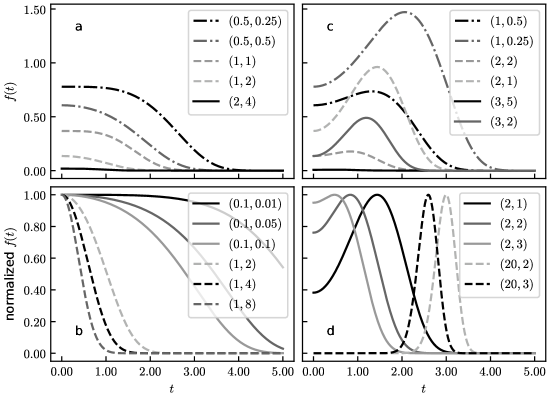
Figure 1: Shape of $f_{v,x}(x)$: two top panels (a, c) are $f_{v,x}(t)$ and two bottom panels (b, d) present the normalized form $f_{v,x}(t)/f_{v,x}(t)$. The two numbers in the legend are the order $v$ and argument $x$. The left and right panels (a, b) and (c, d) present examples with peaks at $t=0$, and $t>0$, respectively.

When integrating $f_{v,x}(t)$ numerically, we sololy need to consider the region where $g_{v,x}(t)\geq\epsilon g_{v,x}(t_{p})$, in which $g_{v,x}(t)$ takes the maximum value at $t_{p}$ and $\epsilon$ denotes the machine epsilon. In fact, from the shape of $g_{v,x}(t)$, the region that satisfies the condition can be defined as a single continuous range as:

$$[t_{0},t_{1}] =\left\{t\,\middle|\,f_{v,x}(t)\geq\epsilon f_{v,x}(t_{p})\right\}$$ (7)

$$=\left\{t\,\middle|\,g_{v,x}(t)\geq g_{v,x}(t_{p})+\log\epsilon\right\}.$$ (8)

2.2 Find peak $t_{p}$

To determine the integral range, we first find the maximum value. In the case of $v^{2}\leq x$, $t_{p}=0$ is obvious from the shape of $g_{v,x}(t)$. In the case of $v^{2}>x$, $g_{v,x}(t)$ exibits the maximum at $t_{p}>0$.

To search for $t_{p}>0$, first, the range where the zero point $t_{p}$ of $g^{\prime}_{v,x}(t_{p})=0$ exists is determined using the property that $g^{\prime}_{v,x}>0$ for $t<t_{p}$ and $g^{\prime}_{v,x}(t)<0$ for $t>t_{p}$. Specifically, for $m\in\mathbb{Z}$, to $[2^{m-1},2^{m}]$ find the smallest $m$, such that $g^{\prime}_{v,x}(2^{m})<0$. The details of this procedure (FindRange) are provided in Algorithm 1.

Algorithm 1 Find range method

1:$g(t_{0})\geq 0$

2:function FindRange($g,t_{0}$) $\triangleright$ return $t_{*}\geq t_{0}$, such that $g(t_{*})<0$

3:     $m\leftarrow 0$

4:     while $g(t_{0}+2^{m+1})\geq 0$ do

5:         $m\leftarrow m+1$      

6:     return $t_{0}+2^{m}$, $t_{0}+2^{m+1}$

Next, for the obtained existence range $[2^{m-1},2^{m}]$, find $t_{p}$, such that $f^{\prime}(t_{p})=0$, using a combination of the binary search and Newton methods. The details of this procedure (FindZero) are provided in Algorithm 2.

Algorithm 2 Modified Newton Method

1:$g(t_{0})>0$, $g(t_{1})<0$

2:function FindZero($g,t_{0},t_{1}$) $\triangleright$ return $t_{0}\leq t_{*}\leq t_{1}$, such that $g(t_{*})=0$

3:     $t_{0}^{(0)},t_{1}^{(0)},i\leftarrow t_{0},t_{1},0$

4:     repeat$\triangleright$ $\text{tol}=1$ and $\text{max\_iter}=10$

5:         $t_{\text{shrink}}\leftarrow t_{0}^{(i)}+(t_{1}^{(i)}-t_{0}^{(i)})/2$$\triangleright$ Binary search

6:         $t_{\text{newton}}\leftarrow\textsc{Clip}(t_{0}^{i+1}-g(t_{0}^{(i)})/g^{\prime}(t_{0}^{(i)}),t_{0},t_{\text{shrink}})$ $\triangleright$ Newton method

7:         if $g(t_{\text{shrink}})<0$ then

8:              $t_{0}^{(i+1)},t_{1}^{(i+1)}\leftarrow t_{\text{shrink}},t_{1}^{(i)}$

9:         else if $g(t_{\text{newton}})<0$ then

10:              $t_{0}^{(i+1)},t_{1}^{(i+1)}\leftarrow t_{\text{newton}},t_{\text{shrink}}$

11:         else

12:              $t_{0}^{(i+1)},t_{1}^{(i+1)}\leftarrow t_{0}^{(i)},t_{\text{newton}}$          

13:         $i\leftarrow i+1$

14:     until $|t_{0}^{i}-t_{0}^{i-1}|<\text{tol}$ and $i<\text{max\_iter}$

15:     return $t_{0}^{(i)}$

2.3 Find the integration range $[t_{0},t_{1}]$

In the cases of $v^{2}\leq x$ or of $v^{2}>x$ and $f(0)-\epsilon f(t_{p})>0$, $t_{0}=0$ from the shape of $f_{v,x}(t)$. Otherwise, FindZero is applied within the range $[t_{0},t_{p}]$ to obtain $t_{0}$, such that $g_{v,x}(t_{0})-g_{v,x}(t_{p})-\log\epsilon=0$.

For $t_{1}$, after applying FindRange to determine the range $[t_{p}+2^{m-1},t_{p}+2^{m}]$, apply FindZero within the range to obtain $t_{1}$, such that $g_{v,x}(t_{1})-g_{v,x}(t_{p})-\log\epsilon=0$.

2.4 Integration

After obtaining $t_{0}$ and $t_{1}$, integrate numerically over the range with the fixed number of divisions $n$:

$$K_{v}(x)\sim h\sum_{m=0}^{n}c_{m}f_{v,x}\left(t_{m}\right),$$ (9)

where

$$h=\frac{t_{1}-t_{0}}{n},\quad t_{m}=t_{0}+mh,$$ (10)

$$c_{0}=c_{n}=1/2,\quad c_{m}=1\,\,(m=1,\ldots,n-1).$$ (11)

In fact, for numerical stability, log_sum_exp was applied to $g_{v,x}(t_{m})$:

$$\log K_{v}(x)\sim g_{v,x}(t_{p})+\log\sum_{m=0}^{n}h\exp\left\{c_{m}\left(g_{v,x}(t_{m})-g_{v,x}(t_{p})\right)\right\}.$$ (12)

2.5 Implementation

The entire proposed algorithm based on integration, which is hereafter denoted as ”I,” is summarized in Algorithm 3. Our implementations using Python and TensorFlow are available at https://github.com/tk2lab/logbesselk. In section 3, the proposed method is compared with implementations by series expansion (”S;” see A), continued fraction (”C;” see B), and asymptotic expansion (”A;” see C). The implementations adopted for the comparison are also available. These implementations used for the comparison are also publicly available at the same already provided url.

Algorithm 3 Main algorithm of logbesselk

1:function LogBesselK($v,x$) $\triangleright$ return $\log K_{v}(x)$

2:     $t_{p}\leftarrow 0$

3:     if $g^{\prime\prime}_{v,x}(0)>0$ then$\triangleright$ find $t_{p}>0$

4:         $t_{s},t_{e}\leftarrow\textsc{FindRange}(g^{\prime}_{v,x}(t),0)$

5:         $t_{p}\leftarrow\textsc{FindZero}(g^{\prime}_{v,x}(t),t_{e},t_{s})$      

6:     $t_{0}\leftarrow 0$

7:     if $g_{v,x}(0)-g_{v,x}(t_{p})\leq\log\epsilon$ then$\triangleright$ find $0<t_{0}\leq t_{p}$

8:         $t_{0}\leftarrow\textsc{FindZero}(g_{v,x}(t)-g_{v,x}(t_{p})-\log\epsilon,0,t_{p})$      

9:     $t_{s},t_{e}\leftarrow\textsc{FindRange}(g_{v,x}(t)-g_{v,x}(t_{p})-\log\epsilon,t_{p})$

10:     $t_{1}\leftarrow\textsc{FindZEro}(g_{v,x}(t)-g_{v,x}(t_{p})-\log\epsilon,t_{e},t_{s})$ $\triangleright$ find $t_{1}>t_{p}$

11:     return $\int_{t_{0}}^{t_{1}}g_{v,x}(t)dt$$\triangleright$ see (12)

3 Evaluation

We adopted the calculations by Mathematica (Walfram) as an accurate reference to evaluate accuracy in the range $v\in[0,99]$, $x\in[10^{-1},10^{2.1}]$. In this study, the errors were evaluated using $\log_{10}\left(|\Delta|/\epsilon+1\right)$, where $\Delta$ is the deviation from the reference. The experiments are conducted in the following environment: Intel(R) Xeon(R) W-2123 3.60GHz CPU, 128GB memory, NVIDIA TITAN RTX GPU, Ubuntu 20.04.2 LTS, Python 3.8.10, and TensorFlow 2.6.0.

3.1 Accuracy

We first evaluate the accuracy of the methods based on series expansion (S), continued fraction (C), asymptotic expansion (A), and integration (I). In the region near $v=x$, the accuracy of these methods deteriorates [19]. It can be deduced that series expansion is accurate for $x<5$, continued fraction is accurate for $x>1$, and asymptotic expansion is accurate in the range $v>10$ or $x>10$ (Fig. 2). However, there is no region where integration is inaccurate.

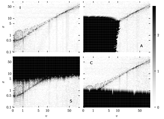
Figure 2: Error corresponding to order $v$ and argument $x$: I) the proposed integration method; S) series expansion method; C) continued fraction method; A) asymptotic expansion method. Error is defined by $\log(|\Delta|/\epsilon+1)$, where $\Delta$ denotes the deviation from the reference.

3.2 Computational time

Next, we examined the computation time for each order $v$ and argument $x$ separately. The computation time was obtained by excluding regions with errors of 4 or more. For I, the computation time tends to be generally uniform; however, for S, C, and A, there are regions in the domain where the computation time becomes large (Fig. 3).

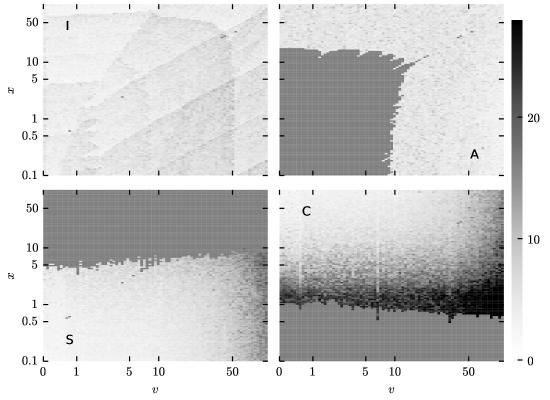
Figure 3: Computational time (msec) corresponding to order $v$ and argument $x$: I) the proposed integration method; S) series expansion method; C) continued fraction method; A) asymptotic expansion method. The computation time is not measured in the gray area because of the large error.

Although TensorFlow can compute multiple pairs of $v$ and $x$ simultaneously, the computation time in this case is the worst computation time for the included $v$ and $x$. Therefore, the worst-case computation time within the range assumed in the application is required to be small, instead of the average computation time.

3.3 Combinations

For each value of $v$ and $x$, the method with the highest accuracy among S, C, and A was identified. The results demonstrated that S and C were separated by the value of $x$. In contrast, A and S+C are distributed in the same region were sparsely and are considered to be equal in terms of accuracy (Fig. 4a). The criterion for separating S and C was set to $x=1.6+0.5\log(x+1)$.

We also examined the method with the shortest computation time under the condition that the error is less than one. Accordingly, the regions of S, C, and A were clearly separated (Fig. 4b). The criterion for separating S+C and A was $v=25$.

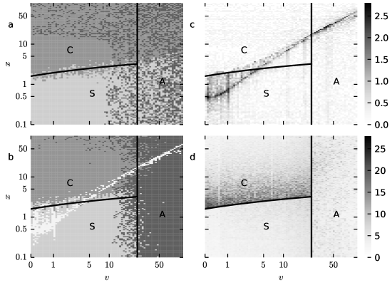
Figure 4: a) Among S, C, and A, the region with the best accuracy for S is depicted in red, the region with the best accuracy for C is in blue, and the region with the best accuracy for A is in green. b) Among S, C, and A, the method with the smallest computation time is shown for the condition that error is less than 1. c, d) Evaluation of theoretical error (c) and computation time (d) by combining S, C, and A.

When the regions were defined in such a way that the accuracy was high and the computation time was short, sufficient results were obtained for the accuracy (Fig. 4c); however, for the computation time, there were regions near the boundary in which the computation was slow (Fig. 4d).

3.4 Advantage of the proposed method

We compared the proposed method with combinations of S, C, and A. Here, in addition to our own implementation of the combination, we also compared the proposed methods with TensorFlowProbability (tfp), an existing implementation of the same combination.

No significant difference in accuracy existed for a wide range of $v$ and $x$. The distribution of errors was not substantially different among methods (Fig. 5a). In addition, the distribution of the errors was not significantly different among the methods, and the mean value was the smallest for the proposed method (Fig. 5b).

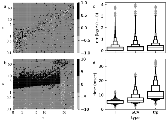
Figure 5: Comparison between the proposed method I and the SCA combination: difference in error (a) and computation time (b). Distribution of error (c) and computation time (d). tfp presents the results of TensorflowProbability.

Regarding execution time, the proposed method exhibited a higher performance in a wide range (Fig. 5c). The computation times were stable at approximately 5 ms, which indicates that it outperforms the other methods (Fig. 5d).

Next, we performed vectorized computations on arrays of various sizes and measured the computation time. Orders $v$ and arguments $x$ were generated in the range $[0,99]$ as $10^{2r}-1$, and $[0.1,100]$ as $10^{3r-1}$, respectively, where $r$ denotes a uniform random number. In this case, the proposed method could compute from an array size of $10^{1}$ up to $10^{4}$, with almost no change in computation time (Fig. 6). The increase in computation time above $10^{4}$ can be attributed to the fact that the memory limit was reached.

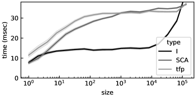
Figure 6: Computation time for parallel computing.

For the SCA and tfp implementations, the computation time increases in the region up to $10^{2}$, and then becomes almost constant (Fig. 6). This can be expected to depend on the probability of including combinations with slow computation speed. As aforementioned, the execution time of a vectorized computation corresponds to the worst-case computational complexity of the included computations; and the computation times of SCA and tfp vary for the combination of $v$ and $x$ (Fig. 5cd).

4 Discussion

4.1 Derivatives

The derivative of the Bessel function $K_{v}(x)$ with respect to the argument $x$ is given by

$$\frac{\partial K_{v}}{\partial x}=-\frac{v}{x}-\frac{K_{v-1}(x)}{K_{v}(x)}.$$ (13)

The derivatives to $x$ of SCA and tfp are calculated using Eq. 13. However, the derivative with respect to order $v$ is not provided by most libraries, and there is no known approach to obtain it indirectly.

The derivatives of the Bessel function $K_{v}(x)$ with respect to the order $v$ and the argument $x$ are obtained by differentiating $f_{v,x}(t)$ and integrating with $t$. The derivatives of $f_{v,x}(t)$ are given by

$$\log(-1)^{m}f_{v,x}^{(n,m)}(t)=\begin{cases}n\log t+m\log\cosh(t)+\log\cosh\left(vt\right)&n~{}\text{is even}\\ n\log t+m\log\cosh(t)+\log\sinh\left(vt\right)&n~{}\text{is odd}\end{cases},$$ (14)

and these also have the single range that should be integrated as the $f_{v,x}(t)$ case. Therefore, the derivatives of $K_{v}(x)$ can be obtained similarly to those of $K_{v}(x)$.

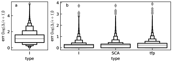
Figure 7: Differentiation errors in $v$ (a) and $x$ (b), respectively.

The derivative with respect to $x$ can be calculated with an error less than one, as $K_{v}(x)$ (Fig. 7a). For the derivative with respect to $v$, the mean of the error is greater than one, which indicates that the accuracy is low. This could be attributed to the presence of the log term in the function to be integrated, and it is believed that the behavior around zero is incompletely captured. Nevertheless, the relative error is approximately $10^{1}4$, which is sufficiently useful, considering that it can be calculated fast.

4.2 Low precision floating point

Experiments were also conducted on 32-bit low-precision floating-point systems, and results of less than $1\epsilon$ were obtained in most regions. The computation time was almost half that of the 64-bit case, and the overall trend was also consistent.

5 Conclusion

We have proposed a computational method suitable for the parallel computation of Bessel functions. The proposed method is a simple method that adds a preprocessing step to efficiently refine the integration range to the approach of computing the integral representation. Accordingly, the proposed method enables fast computation with sufficient accuracy.

This method is also applicable to the differentiation of Bessel functions, and is effective in various fields such as mathematics, physics, and statistics. In the future, it will be beneficial to investigate faster methods for the parallel processing of several related special functions.

Appendix A Series expansion

When $|u|\leq 1/2$ and $x$ is small, $K_{u}(x)$ can be expanded into a series [8]:

$$K_{u}(x)=\sum_{n=0}^{\infty}\frac{1}{n!}\left(\frac{x}{2}\right)^{2n}f_{n},\quad K_{u+1}(x)=\sum_{n=0}^{\infty}\frac{1}{n!}\left(\frac{x}{2}\right)^{2n-1}g_{n},$$ (15)

where

$$f_{n}=\frac{\pi}{2\sin u\pi}\left\{\left(\frac{x}{2}\right)^{-u}\Gamma(n+1-u)^{-1}-\left(\frac{x}{2}\right)^{u}\Gamma(N+1+u)^{-1}\right\},$$ (16)

$$g_{n}=p_{n}-nf_{n},\quad p_{n}=\frac{1}{2\left(n-u\right)!}\left(\frac{x}{2}\right)^{-u}\Gamma(1+u)^{-1}.$$ (17)

The coefficients $f_{n}$, $p_{n}$, and $q_{n}$ can be obtained via forward recursion:

$$f_{n}=\frac{nf_{n-1}+p_{n}+q_{n}}{n^{2}+u^{2}},\quad p_{n}=\frac{p_{n-1}}{n-u},\quad q_{n}=\frac{q_{n-1}}{n+u}.$$ (18)

$K_{v}(x)$ = $K_{n+u}(x)$ is recursively obtained from $K_{u}$ and $K_{u+1}$:

$$K_{u+1}=\frac{2u}{x}K_{u}+K_{u-1}.$$ (19)

Appendix B Continued fraction method

Using a sequence of numbers $p_{n}$ containing hypergeometric functions [8, 11]

$$p_{n}=(2x)^{n}{}_{2}F_{0}\left(u+n+\frac{1}{2};u-n-\frac{1}{2};-2x\right)\\ =\sum_{m=0}^{\infty}\frac{(2x)^{n+m}}{m!}\prod_{i=1}^{m}\left\{\left(n+i-\frac{1}{2}\right)^{2}-u^{2}\right\},$$ (20)

the Bessel function $K_{u}(x)$ for a large $x$ can be defined as:

$$K_{u}(x)=\sqrt{\frac{\pi}{2x}}e^{-x}p_{0}.$$ (21)

From the derivative of $p_{0}$ and $K_{u}(x)$, an adjacent value $K_{u+1}(x)$ is also given by

$$K_{u+1}(x)=\left\{\frac{1}{x}\left(\frac{1}{2}+v+x\right)+\frac{a_{1}}{x}\frac{p_{1}}{p_{0}}\right\}K_{u}(x).$$ (22)

The value of $K_{v}(x)$ for any order $v=n+u$ can be obtained recursively, similar to the series expansion case.

From an asymptotic expression for $p_{n}$

$$p_{n-1}=b_{n}p_{n}-a_{n+1}p_{n+1},$$ (23)

$$a_{n}=\left(n-\frac{1}{2}\right)^{2}-u^{2},\quad b_{n}=2(x+n),$$ (24)

the ratio $q_{n}=p_{n}/p_{0}$ can be calculated recursively:

$$q_{-1}=0,\quad q_{0}=1,\quad q_{n+1}=\frac{q_{n-1}-b_{n}q_{n}}{a_{n+1}}.$$ (25)

The ratios of adjacent $p_{n}$ are also represented using Steel’s method:

$$c_{1}=\frac{1}{b_{1}},\quad c_{n+1}=\frac{1}{b_{n+1}-a_{n+1}c_{n}},$$ (26)

$$r_{1}=\frac{1}{b_{1}},\quad r_{n+1}=r_{n}(b_{n+1}c_{n+1}-1),$$ (27)

$$\frac{p_{n}}{p_{n-1}}=\sum_{m=n-1}^{\infty}r_{m}.$$ (28)

From Temme’s rule

$$\sum_{m=0}^{\infty}d_{m}p_{m}=1,\quad d_{n}=\frac{1}{n!}\prod_{m=1}^{n}a_{m},$$ (29)

we can calculate $p_{0}$ from $d_{n}$, $r_{n}$, and $p_{n}$:

$$p_{0}=p_{0}\left(\sum_{n=0}^{\infty}d_{n}p_{n}\right)^{-1}=\left(1+\sum_{n=1}^{\infty}d_{n}\frac{p_{n-1}}{p_{0}}\frac{p_{n}}{p_{n-1}}\right)^{-1}\\ =\left(1+\sum_{n=1}^{\infty}d_{n}q_{n}\sum_{m=n-1}^{\infty}r_{m}\right)^{-1}=\left(1+\sum_{m=0}^{\infty}r_{m}\sum_{n=1}^{m}d_{n}q_{n}\right)^{-1}.$$ (30)

Appendix C Asymptotic expansion

The expansion in terms of the harmonic functions for $K_{v}(x)$ is given by [12]

$$K_{v}(x)=\sqrt{\frac{\pi}{2p}}\left(\frac{v+p}{x}\right)^{v}e^{-p}\sum_{i=0}^{\infty}\sum_{j=0}^{i}c_{i,j}p^{-i}q^{j},$$ (31)

$$p=\sqrt{v^{2}+x^{2}},\quad q=\frac{v^{2}}{v^{2}+x^{2}}.$$ (32)

The coefficients $c_{i,j}$ can be evaluated using a recurrence relationship:

$$c_{i+1,j}=\left(\frac{k-2}{2}+\frac{5}{8(k+1)}\right)c_{i,j-1}-\left(\frac{k}{2}+\frac{1}{8(k+1)}\right)c_{i,j},$$ (33)

$$i=0,\dots,\quad j=0,\dots,i+1,\quad k=i+2j,$$ (34)

$$c_{0,-1}=c_{0,1}=0,\quad c_{0,0}=1.$$ (35)

References

- [1] G. N. Watson, A treatise on the theory of Bessel functions, Cambridge University Press, Cambridge, 1922.
- [2] O. E. Barndorff-Nielsen, Processes of normal inverse gaussian type, Finance and stochastics 2 (1) (1997) 41–68.
- [3] O. E. Barndorff-Nielsen, Normal inverse gaussian distributions and stochastic volatility modelling, Scandinavian Journal of statistics 24 (1) (1997) 1–13.
- [4] A. R. Hassan, M. I. H. Bhuiyan, An automated method for sleep staging from eeg signals using normal inverse gaussian parameters and adaptive boosting, Neurocomputing 219 (2017) 76–87.
- [5] A. B. Das, M. I. H. Bhuiyan, S. S. Alam, Classification of eeg signals using normal inverse gaussian parameters in the dual-tree complex wavelet transform domain for seizure detection, Signal, Image and Video Processing 10 (2) (2016) 259–266.
- [6] A. O’Hagan, T. B. Murphy, I. C. Gormley, P. D. McNicholas, D. Karlis, Clustering with the multivariate normal inverse gaussian distribution, Computational Statistics & Data Analysis 93 (2016) 18–30.
- [7] T. Takekawa, Clustering of non-gaussian data by variational bayes for normal inverse gaussian mixture models, arXiv preprint arXiv:2009.06002 (2020).
- [8] N. Temme, On the numerical evaluation of the modified Bessel function of the third kind, Journal of Computational Physics 19 (1975) 324.
- [9] D. E. Amos, Computation of modified Bessel functions and their ratios, Mathematics of Computation 28 (1974) 239–251.
- [10] J. B. Campbell, On Temme’s algorithm for the modified Bessel function of the third kind, ACM Trans. Math. Softw. 6 (4) (1980) 581––586. doi:10.1145/355921.355928.
- [11] I. J. Thompson, A. R. Barnett, Modified Bessel functions and of real order and complex argument, to selected accuracy, Computer Physics Communications 47 (1987) 245–257.
- [12] F. W. J. Olver, Asymptotics and special functions, Academic Press, 1974, reprinted as AKP Classics A.K. Peters Ltd., Wellesley , MA, 1997.
- [13] F. W. J. Olver, L. C. Maximon, Bessel functions, https://dlmf.nist.gov/10, digital Library of Mathematics Functions.
- [14] M. Galassi, et al., GNU scientific library reference manual (3rd ed.), Software available from https://www.gnu.org/software/gsl/.
- [15] J. Maddock, P. Bristow, H. Holin, X. Zhang, Boost C++ Libraries, Math/Special Functions, Reference available from https://www.boost.org/doc/libs/1_77_0/libs/math/doc/html/math_toolkit/bessel/mbessel.html (2008).
- [16] J. V. Dillon, I. Langmore, D. Tran, E. Brevdo, S. Vasudevan, D. Moore, B. Patton, A. Alemi, M. Hoffman, R. A. Saurous, Tensorflow distributions, Software available from https://www.tensorflow.org/probability/ (2017). arXiv:arXiv:1711.10604.
- [17] C. Schwartz, Numerical calculation of Bessel functions, International Journal of Modern Physics C 23 (12) (2012) 1250084. doi:10.1142/S0129183112500842.
- [18] M. Abadi, et al., TensorFlow: Large-scale machine learning on heterogeneous systems, Software available from https://www.tensorflow.org (2015).
- [19] A. Gil, J. Segura, N. M. Temme, Computation of the modified Bessel function of the third kind of imaginary orders: uniform Airy-type asymptotic expansion, Journal of Computational and Applied Mathematics 153 (2003) 225–234.