Lies My Teacher Told Me About Density Functional Theory: Seeing Through Them with the Hubbard Dimer

Abstract

Most realistic calculations of moderately correlated materials begin with a ground-state density functional theory (DFT) calculation. While Kohn-Sham DFT is used in about 40,000 scientific papers each year, the fundamental underpinnings are not widely appreciated. In this chapter, we analyze the inherent characteristics of DFT in their simplest form, using the asymmetric Hubbard dimer as an illustrative model. We begin by working through the core tenets of DFT, explaining what the exact ground-state density functional yields and does not yield. Given the relative simplicity of the system, almost all properties of the exact exchange-correlation functional are readily visualized and plotted. Key concepts include the Kohn-Sham scheme, the behavior of the XC potential as correlations become very strong, the derivative discontinuity and the difference between KS gaps and true charge gaps, and how to extract optical excitations using time-dependent DFT. By the end of this text and accompanying exercises, the reader will improve their ability to both explain and visualize the concepts of DFT, as well as better understand where others may go wrong. This chapter appears in the book Autumn School on Correlated Electrons: Simulating Correlations with Computers (2021) prepared by Forschungszentrum Jülich.

1 Introduction

Density functional theory (DFT) is an extremely sophisticated approach to many-body problems Mahan (2000); Blöchl (2011). It must be among the most used and least understood of all successful theories in physics. Currently, about 50,000 papers each year report results of Kohn-Sham (KS) DFT calculations Pribram-Jones et al. (2015), including room temperature superconductors under high pressure Pickard et al. (2020), heterogeneous catalysis at metal surfaces and for nanoparticles Nørskov et al. (2011), understanding the interior of Jupiter and exoplanets Zeng et al. (2019), studying how ocean acidification affects the seabream population Velez et al. (2019), and even which water to use when making coffee Hendon et al. (2014).

But much of modern condensed matter physics involves using model Hamiltonians to study strongly correlated systems, where understanding new phenomena is considered far more important than generating accurate materials-specific properties Lechermann (2011); Solovyev (2008). In fact, our standard diagrammatic approach (expansions in the strength of the electron-electron coupling) is hard-wired into all our descriptions of such many-body phenomena, be it the fractional quantum Hall effect Tsui et al. (1982) or the Kondo effect (even when perturbation theory fails, we still think of resummed diagrams) Kondo (1964).

Because DFT is logically subtle, without requiring much mathematical gymnastics (although they are available for those that enjoy them Lieb (1983)) or skill with summing Feynman diagrams, and because DFT is entirely different from the standard approach, most of what you may have learned is hopelessly confused or simply downright untrue. Hence the title of this article, taken from a popular book on history Loewen (2008). For example, any conflation of the KS scheme with traditional mean-field theory is a dire mistake, and should be avoided at all costs.

This chapter is primarily designed to explain essential concepts of DFT to theorists more familiar with standard many-body theory and perhaps more experienced in dealing with strongly correlated systems. It should also prove useful for anyone performing DFT calculations on weakly correlated systems, who might be wondering where things go wrong as correlations grow stronger. Additionally, the Hubbard dimer is a wonderful teaching tool for basic concepts, as so many of its exact results can be derived analytically.

The first use of this material came in a conversation between KB and Duncan Haldane at a meeting sponsored by the US Department of Energy. Duncan asked KB to explain this DFT business, and he suggested the dimer as the minimal relevant model. After 45 minutes of tough argument, Haldane said “That’s the first time I’ve ever really understood this Kohn-Sham scheme. Thanks.” Within 2 years, he was awarded a share in a Nobel Prize in physics Haldane (2017). While correlation is not causation, Haldane did not win his share until after he understood KS-DFT with the aid of this simple model!

However, it is important to note that the benefits of this type of analysis are not solely limited to those working in theoretical physics. In the fields of theoretical chemistry and material science, for instance, where ground-state electronic energies are often required to be extremely accurate Lee and Scuseria (1995); Feller and Peterson (2007); Vuckovic et al. (2019), there has been growing technological interest in the study of both chemically complex and strongly correlated materials Hafner et al. (2011); O’Regan and Grätzel (1991). This chapter was partly designed with these fields in mind, serving as a resource for any computational scientist who wishes to better comprehend the limitations of their computational methods. Throughout this text, there will be various highlighted sections dedicated to examples, exercises, and key concepts to aid the reader in applying what is learned in this study to their own endeavors.

There are now a huge number of diverse introductions to DFT, with many different perspectives. These include a simple tutorial for anyone with knowledge of quantum mechanics Burke and Wagner (2013), a very long online textbook with lots of nasty problems Burke (2007), a many-body introduction Dreizler and Gross (1989), and even video lectures de Calcul Atomique et Moléculaire . But this chapter is specifically aimed at explaining the most essential concepts, and why strongly correlated systems are more challenging in DFT. All the Hubbard material appears in two long review articles, one on the ground state theory Carrascal et al. (2015) and a second on linear-response TDDFT Carrascal et al. (2018). The Hubbard dimer has been recently used to explore effects in other aspects of DFT, such as magnetic DFT Ullrich (2018), ensemble DFT Sagredo and Burke (2018), and thermal DFT Sagredo and Burke (2020).

1.1 Background

We work in the non-relativistic non-magnetic Born-Oppenheimer approximation, using Hartree atomic units ($e^{2}=\hbar=m_{e}=1$). The Hamiltonian for the electrons is simple and known exactly

$$\hat{H}=\hat{T}+\hat{V}_{\rm ee}+\hat{V}\!,$$ (1)

where $\hat{T}$ is their kinetic energy, $\hat{V}_{\rm ee}$ is the electron-electron Coulomb repulsion, and $\hat{V}$ is the one-body potential, equal to a sum of Coulomb attractions to the ions in an isolated molecule or solid. We let $N$ be the number of electrons.

A first-principles approach to this problem is to feed a computer a list of nuclear types and positions and, following a recipe, it spits out various properties of the electronic system. In quantum chemistry Szabo and Ostlund (1996), the recipe is called a model chemistry Ochterski et al. (1995); Bartlett and Musial (2007) if both the method (e.g. Hartree-Fock) and the basis set are specified.

We contrast this with traditional approaches in condensed matter Girvin and Yang (2019). Often a model Hamiltonian is written down, hoping that it describes the dominant physical effects. For most interesting problems, standard approaches to solving this Hamiltonian will fail, i.e., be hopelessly inadequate or require near-infinite computer resources. An inspired approximation may be found that works well enough, and so the underlying physics can be explained. Well enough will usually mean that with good estimates of the model parameters, qualitative and even semi-quantitative agreement is found with key properties of interest.

Each of these are excellent approaches, especially for the purposes they were designed for. Modern DFT calculations of weakly correlated materials (and molecules) are of the first-principles type, and often yield atomic positions within 1-2 hundredths of an Ångstrom and phonon frequencies within 10%, without any materials-specific input, an impossibility with a simple model Hamiltonian. On the other hand, with standard approximations, DFT calculations always fail whenever a bond such as H₂ is stretched, and correlations become strong Cohen et al. (2008). Even simple Mott-Hubbard physics is beyond such methods (and we shall see why in this chapter), or Kondo physics (but see Reference Jacob et al. (2020)).

But more and more of modern materials research requires the intelligent application of both approaches, and many methods, such as DFT+U Himmetoglu et al. (2014) or dynamical mean field theory (DMFT) Anisimov et al. (1997); Kotliar et al. (2006); Vollhardt (2011); Pavarini (2011) are being developed to bridge the gap. Many of the materials of greatest practical interest to energy research (such as for batteries Hafner et al. (2011) or photovoltaics O’Regan and Grätzel (1991)) include a moderate level of correlation that require a pure DFT approach to be enhanced, by adding vital missing ingredients of the physics.

The US and Britain are friends ‘separated by a common language’ Wilde (1887). This is essentially true of the mass of confusion between traditional many-body theory and DFT. In DFT, we use the same words as in MBT, but giving them different meanings, simply because we enjoy confusing folks.

Finally, we mention an intermediate Hamiltonian between the dazzling complexity of the real physical and chemical world and the beautiful simplicity of the Hubbard model. A great challenge to studying the effects of strong correlation has been the difficulty in producing highly accurate benchmark data. Molecular electronic structure calculations are much simpler than materials calculations, and quantum chemistry has long been able to provide highly accurate answers for many small molecules at or near equilibrium Bartlett and Musial (2007), as well as the complete binding energy curves of others Harriman (1986). But this is much harder to do for materials. Recent illustrations of this difficulty are the careful bench-marking of model Hamiltonians (such as an $8{\times}8$ Hubbard lattice) using highly accurate many-body solvers LeBlanc et al. (2015), the amount of computation needed to find an accurate cohesive energy of the benzene crystal Yang et al. (2014), and the celebration of merely being able to agree on approximate DFT results with a variety of solid-state codes Lejaeghere et al. (2016).

To overcome this difficulty, about 10 years ago, a mimic of realistic electronic structure calculations was established Stoudenmire et al. (2012). This mimic uses potentials that are defined continuously in space (i.e., not a lattice model) but are one-dimensional. In fact, ultimately, a single exponential was chosen Baker et al. (2015), whose details mimic those of the popular soft Coulomb potential. With about 20 grid points per ‘atom’, standard density-matrix renormalization (DMRG) methods White (1992, 1993) could then rapidly produce extremely accurate ground-state energies and densities for chains of up to about 100 atoms Stoudenmire et al. (2012). By living in 1D, not only is DMRG very efficient, but the thermodynamic limit (of the number of atoms going to infinity with fixed interatomic spacing) is also reached much more quickly than in 3D. Moreover, the parameters were chosen so that standard density functional approximations, such as the local density approximation Kohn and Sham (1965), succeeded and failed in ways that were qualitatively similar to those in the real world Wagner et al. (2012). We will refer to this 1D laboratory for further demonstration of some of the simple results shown in this chapter.

1.2 Hubbard dimer

The Hubbard model (in 1, 2 or 3D) Hubbard (1963) is the standard model for studying the effects of strong correlation on electrons. By default, it implies an infinite periodic array of sites. For our demonstration, we simply need two sites. We have $N=2$ and the ground-state is always a singlet. The Hamiltonian (in 2nd quantization) is

$${\hat{H}}=-t\sum_{\sigma}\left(\hat{c}_{1\sigma}^{\dagger}\hat{c}_{2\sigma}+h.c.\right)+U\sum_{i}\hat{n}_{i\uparrow\,}\hat{n}_{i\downarrow}+\sum_{i}v_{i}\hat{n}_{i}\,.$$ (2)

The kinetic term is just hopping between the sites, and is the discretization of the kinetic operator on the lattice, with the diagonal elements set to 0. The electron-electron repulsion is just an onsite $U\!$, while the one-body operator is just an on-site potential, $v_{1}$ and $v_{2}$.

In this chapter, we imagine a world in which Eq. (1) is replaced by Eq. (2), i.e., as if the many-body problem to be solved is simply that of Eq. (2). So, for us, the Hubbard dimer is not an approximation to anything. We will choose the values of $U\!$, $t$, and $v_{i}$ as we wish, to explore various regimes in the model. Any question concerning the origins of these values in terms of realistic orbitals and matrix elements is irrelevant to our work here.

Since a constant in the potential is just a shift in the energy, we set $v_{2}{\,=\,}{-}v_{1}$ and use the parameter $\mathrm{\Delta}v{\,=\,}v_{2}{-}v_{1}$ as the sole determinant of the potential of our system. Similarly, with $N{\,=\,}2$, $n_{2}{\,=\,}N{-}n_{1}$, and we use $\mathrm{\Delta}n{\,=\,}n_{2}{-}n_{1}$ as the single parameter characterizing the ground-state density. Thus ground-state DFT in this model is simply site-occupation function theory (SOFT) and density functionals are replaced by simple functions of a single variable, $\mathrm{\Delta}n$. Finally, we choose $t{\,=\,}1/2$ and report all variables in units of $2t$, as one can scale all energies by a constant.

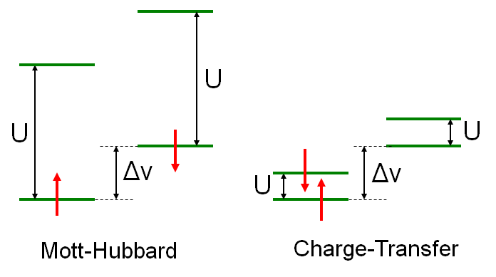
Figure 1: Two distinct regimes of the asymmetric Hubbard dimer. On the left, the charging energy is much greater than the difference in on-site potentials, and the left- and right-occupation numbers are similar. On the right, the situation is reversed, and the occupation on the left is much greater than that of the right. Reproduced from Ref. Carrascal et al. (2015).

Different physics appears depending on the ratio of $U$ to $\mathrm{\Delta}v$, i.e., on-site repulsion versus inhomogeneity, see Fig. 1. When $U{\,\gg\,}\mathrm{\Delta}v$, the system is strongly correlated, with both site occupations close to $1$, despite any inhomogeneity. For $\mathrm{\Delta}v\gg U\!$, the system is weakly correlated, and the on-site $U$ is insufficient to stop one occupation becoming much greater than the other.

For those with a chemical inclination, this is a minimal basis model for a diatomic with $2$ electrons (with some matrix elements and orbital overlap ignored). For H₂, $\mathrm{\Delta}v=0$, but $t$ decreases as the separation between the nuclei is increased, so that $U$ (in units of $2t$) grows exponentially. The ground-state is close to a single Slater determinant near equilibrium ($U{\ll}1$), so that Hartree-Fock (HF) is a reasonable approximation. But $U{\gg}1$ when very stretched, so that the ground-state is now a Heitler-London wavefunction, and (restricted) HF is very poor. The highly unsymmetric case corresponds to HeH⁺, where both electrons reside on the He side, as long as $\mathrm{\Delta}v$ remains larger than $U$ as the bond is stretched.

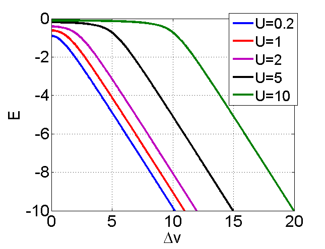
Figure 2: Exact ground-state energy of the Hubbard dimer as a function of $\mathrm{\Delta}v$ for several values of $U\!$.  The qualitative behavior changes as $\mathrm{\Delta}v$ passes through $U\!$. Reproduced from Ref. Carrascal et al. (2015).

There are well-known analytic solutions for all states of the 2-site Hubbard model and the behavior of the ground-state energy Carrascal et al. (2015) is shown in Fig. 2. Simple limits include the symmetric case

$$\hskip 4.30554ptE=-\sqrt{1+(U/2)^{2}}+U/2,~{}~{}~{}~{}~{}\mathrm{\Delta}n=0\hskip 25.83325pt\mbox{SYM}$$ (3)

An expansion of the square root in the symmetric case in powers of $U$ has a radius of convergence of 2, while the opposite expansion in $1/U$ has a radius of 1/2. Thus there is a well-defined critical point at $U{\,=\,}2$, below which perturbation in the electron-electron coupling strength converges, i.e., the system is weakly correlated, and above which it is strongly correlated. Another simple limit is the non-interacting (tight-binding) case ($U{\,=\,}0$)

$$E=-\sqrt{1+\mathrm{\Delta}v^{2}},~{}~{}~{}~{}\mathrm{\Delta}n=-2\,\frac{\mathrm{\Delta}v}{\sqrt{1+\mathrm{\Delta}v^{2}}}\hskip 17.22217pt\mbox{($U{=}0$)}$$ (4)

which is given by the blue curve in the figure. We see from the figure that, on a broad scale, $E\approx-(\mathrm{\Delta}v-U)\,\Theta(\mathrm{\Delta}v-U)$. Explicit formulas exist for all the excited-state energies, wavefunctions, and densities also. Approximations in many different limits are given in the many appendices of Reference Carrascal et al. (2015).

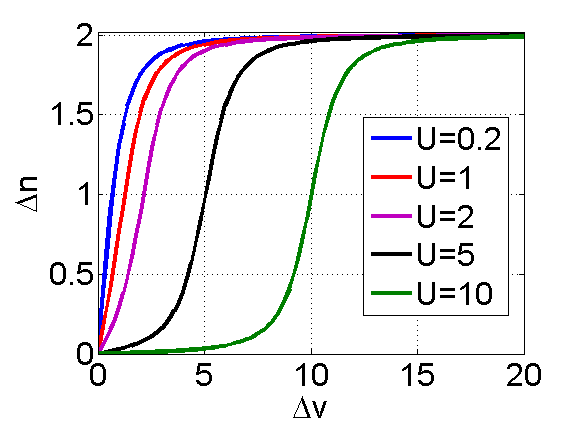
Figure 3: Ground-state occupation of the Hubbard dimer as function of $\mathrm{\Delta}v$ for several values of $U\!$. Reproduced from Ref. Carrascal et al. (2015).

We can also extract any other property we wish from the analytic solution, such as the one-electron density (here the occupations). Fig. 3 shows the ground-state density as a function of $\mathrm{\Delta}v$ for several values of $U\!$.  For any $U\!$,  $n_{2}=n_{1}$ when $\mathrm{\Delta}v=0$. The blue line is essentially the tight-binding solution. In that case, as $\mathrm{\Delta}v$ increases, the occupation difference rapidly increases towards 2. Then, as we turn on $U\!$,  this increase becomes less and less rapid. By the time $U$ reaches 10, the occupations remain close to balanced until $\mathrm{\Delta}v$ becomes close to 10, when (on the scale of $\mathrm{\Delta}v$), it rapidly flips to close to 2.

2 Density functional theory

We have now defined the machinery required to understand the central theorems of DFT through the lens of the Hubbard dimer. The theorems discussed in this section, like their real-space counterparts, are exact and apply directly to ground-state calculations (we will cover time-dependent DFT later). Most DFT calculations are used to determine the ground-state electronic energy of a system, or more specifically, determine the energy of a system as a function of nuclear coordinates. In this section, we will discuss the underlying principles of these calculations by examining their role at the most fundamental level, in their simplest form.

The Hohenberg-Kohn theoremHohenberg and Kohn (1964) is actually three theorems in sequence. These were proved in a simple proof-by-contradiction argument based on the Rayleigh-Ritz variational principle for the wavefunction. Later, the more direct and more general constrained search approach was given by Levy Levy (1982) and Lieb Lieb (1983).

2.1 Hohenberg-Kohn I

HKI proves that the (usual) map of $\mathrm{\Delta}v\to\mathrm{\Delta}n$ is invertible, i.e., $\mathrm{\Delta}n$ is a single-valued function of $\mathrm{\Delta}v$ for a given $U\!$.  This is obvious from Fig. 3 (and its inversion, Fig. 4), and in the TB case

$$\hskip 55.97205pt\mathrm{\Delta}v=\frac{\mathrm{\Delta}n}{\sqrt{4-\mathrm{\Delta}n^{2}}}\hskip 55.97205pt\mbox{($U{=}0$)}.$$ (5)

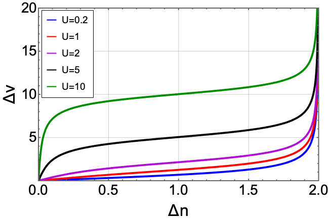
Figure 4: Ground-state potential difference as a function of $\mathrm{\Delta}n$ for several values of $U$.

Fig. 4 is simply Fig. 3 drawn sideways, i.e., with x and y axes reversed. Clearly, for any given value of $U\!$,  there is a unique $\mathrm{\Delta}v$.

A much-stated (but often out of context) corollary of this is that all properties of the system are (implicitly) functionals of $n_{1}$. While this is true, almost all research in DFT focuses on the ground-state energy functional, because it is so useful, and we have few useful approximations for others (e.g., for the first excited-state energy, but see discussion in TDDFT section). Recently, machine learning methods have been trained to find some of these other functionals Moreno et al. (2020, 2021).

2.2 Hohenberg-Kohn II

HKII states that the function below exists and is independent of $\mathrm{\Delta}v$:

$$F_{\scriptscriptstyle\rm U}(n_{1})=\min_{\mathrm{\Psi}\rightarrow n_{1}}{\langle\mathrm{\Psi}|\hat{T}+\hat{V}_{\rm ee}|\mathrm{\Psi}\rangle}=\max_{\mathrm{\Delta}v}\bigg{\{}E(\mathrm{\Delta}v)-\mathrm{\Delta}v\mathrm{\Delta}n/2\bigg{\}}.$$ (6)

where the minimum is over all antisymmetrized normalized 2-electron wavefunctions whose occupation of site 1 is $n_{1}$. The middle expression is the constrained search definition due to Levy Levy (1979). The rightmost form is due to Lieb Lieb (1983). Either definition works here. This $F_{\scriptscriptstyle\rm U}$ functional was termed universal by HK, by which they simply meant that it does not depend on the $\mathrm{\Delta}v$ of your given system, i.e., it is a pure density functional. The phrase, often appearing in the literature, that $F$ is a universal functional, is not meaningful.

Figure 5: Universal part of the energy function(al) of a Hubbard dimer as a function of $n_{1}$ for several values of $U\!$.  As $U$ increases, $F$ tends to $U|1{-}n_{1}|$. Reproduced from Ref. Carrascal et al. (2015).

Although one can write analytic formulas for the ground-state energy for the dimer, there is no explicit analytic formula for $F\!$.  It is trivial to calculate $F$ numerically and $F$ is shown in the Fig. 5. In the special case of $U=0$, it is easy,

$$F_{U=0}(n_{1})=T_{\scriptscriptstyle\rm S}(n_{1})=-\sqrt{n_{1}(2-n_{1})}.$$ (7)

Here we have attached the subscript S to remind us that $U=0$, so this is the kinetic energy function for a single Slater determinant, and is indistinguishable from the blue line of Fig. 5.

2.3 Hohenberg-Kohn III

HKIII states that there is a variational principle for the ground-state energy directly in terms of the density alone:

$$E(\mathrm{\Delta}v)=\min_{n_{1}}\bigg{\{}F_{\scriptscriptstyle\rm U}(n_{1})+\mathrm{\Delta}v\mathrm{\Delta}n/2\bigg{\}}.$$ (8)

This bypasses all the difficulties of approximating the wavefunction (but of course buries them in the definition of $F_{\scriptscriptstyle\rm U}$). Usually, the minimum can be found from the Euler equation

$$\frac{dF_{\scriptscriptstyle\rm U}(n_{1})}{dn_{1}}-\frac{\mathrm{\Delta}v}{2}=0,$$ (9)

and the unique $n_{1}(\mathrm{\Delta}v)$ is the one that satisfies this equation.

This allows us to find a solution to the many-body problem, without ever calculating the wavefunction. Given an expression for $F_{\scriptscriptstyle\rm U}(n_{1})$, either exact or approximate, for any value of $\mathrm{\Delta}v$, one can solve Eq. (9) above to find the corresponding $\mathrm{\Delta}v$ (exact or approximate) and insert into Eq. (8) to find the energy. Any approximation to $F(n_{1})$ provides approximate solutions to all many body problems (every value of $\mathrm{\Delta}v$).

3 Kohn-Sham DFT

The original DFT, called Thomas-Fermi theory Thomas (1927); Fermi (1928), tried to approximate $F_{\scriptscriptstyle\rm U}(n_{1})$ directly, but such direct approximations have never been accurate enough for most electronic structure calculations. A tremendous step forward occurred when Kohn and Sham considered a fictitious system of non-interacting fermions with the same ground-state density as the true many-body one Burke (2012). In our case, this is just the TB problem, for which we already have explicit solutions.

They wrote the $F$ function in terms of quantities that could easily be calculated in such a system:

$$F_{\scriptscriptstyle\rm U}(n_{1})=T_{\scriptscriptstyle\rm S}(n_{1})+U_{\scriptscriptstyle\rm H}(n_{1})+E_{\scriptscriptstyle\rm XC}(n_{1}).$$ (10)

Here, $T_{\scriptscriptstyle\rm S}$ is just the TB hopping energy of Eq. (4), and the Hartree energy is just the mean-field electron-electron repulsion

$$U_{\scriptscriptstyle\rm H}=\frac{U}{2}\big{(}n_{1}^{2}+n_{2}^{2}\big{)},$$ (11)

which is an explicit function of the occupations. Then $E_{\scriptscriptstyle\rm XC}$, the exchange-correlation (XC) energy (about which, much more, later) is simply everything else, i.e., $E_{\scriptscriptstyle\rm XC}$ is defined by Eq. (10). It is then trivial to show, from the Euler equation, that the TB potentials that will reproduce the exact occupations are

$$v_{\scriptscriptstyle\rm{S},i}=v_{i}+Un_{i}+\frac{\partial E_{\scriptscriptstyle\rm XC}}{\partial n_{i}}\,.$$ (12)

The first correction to $v_{i}$ is the Hartree potential, while the second is the XC potential. These KS TB equations must be solved self-consistently, as the potentials depend on the occupations. Once converged, the final densities can be used to extract the total energy of the MB system, via

$$E=T_{\scriptscriptstyle\rm S}+U_{\scriptscriptstyle\rm H}+E_{\scriptscriptstyle\rm XC}+V=\varepsilon-U_{\scriptscriptstyle\rm H}+E_{\scriptscriptstyle\rm XC}-\mathrm{\Delta}v_{\scriptscriptstyle\rm XC}\mathrm{\Delta}n/2\,,$$ (13)

where $\varepsilon$ is the eigenvalue in the TB KS calculation. Again, just like in the HK case, once $E_{\scriptscriptstyle\rm XC}(n_{1})$ is given (either approximate or exact), the KS equations can be solved for any electronic system and a ground-state energy and occupation extracted.

The wondrous improvement due to the KS scheme is that only a small fraction of the total energy (the XC part) need be approximated. Many of the most important quantum effects, such as screening, shell structure, binding energies, etc. are mostly accounted for by the quantum effects of the one-body system. Finally, a very simple, intuitive approximation suggested by KS themselves (the local density approximation (LDA) Dirac (1930); Kohn and Sham (1965)) produced far better results than they expected (but with binding energy errors too large for quantum chemistry taste).

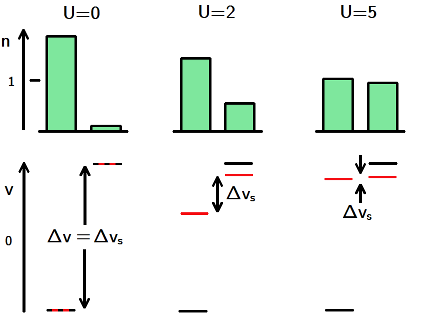
Figure 6: KS DFT view of an asymmetric half-filled Hubbard dimer as a function of $U$. The on-site potential difference $\mathrm{\Delta}v$ is shown in black and the KS on-site potential difference $\mathrm{\Delta}v_{\scriptscriptstyle\rm S}$ is in red. Reproduced from Ref. Carrascal et al. (2015).

Fig. 6 gives us some sense of how this works, for $\mathrm{\Delta}v=1$. Then, if $U=0$, most occupation is on the left. For $U=2$, the repulsion makes the occupations more equal. The KS potential is simply that TB potential that produces those (many-body) occupations. So it must be a smaller potential difference than the real potential. One can see that the Hartree potential will typically overestimate repulsion, while XC corrects that to give the exact answer. Finally, when $U$ is ramped up to 5, the occupations become very close to equal, and the KS potential difference becomes very small.

Traditionally, $E_{\scriptscriptstyle\rm XC}$ is separated into an exchange and a correlation contribution. The exchange contribution is then defined as

$$E_{\scriptscriptstyle\rm X}=\langle\mathrm{\Phi_{\scriptscriptstyle\rm S}}|\hat{V}_{\rm ee}|\mathrm{\Phi_{\scriptscriptstyle\rm S}}\rangle-U_{\scriptscriptstyle\rm H},$$ (14)

where $\Phi_{\scriptscriptstyle\rm S}$ is the KS wavefunction, and $E_{\scriptscriptstyle\rm X}$ is always negative. Then one can show correlation is just

$$E_{\scriptscriptstyle\rm C}=\langle\mathrm{\Psi}|\hat{H}|\mathrm{\Psi}\rangle-\langle\mathrm{\Phi_{\scriptscriptstyle\rm S}}|\hat{H}|\mathrm{\Phi_{\scriptscriptstyle\rm S}}\rangle$$ (15)

and, by the variational principle, is also never positive. These definitions (almost) match those of quantum chemistry Umrigar and Gonze (1994), except that in KS-DFT, all orbitals come from a single potential, while in HF orbitals are freely chosen to minimize the HF energy. But there are some surprises relative to the traditional many-body expansion. For example, because of the definitions, $E_{\scriptscriptstyle\rm X}$ includes some ‘self-exchange’, i.e., it is non-zero even for a single electron (where $E_{\scriptscriptstyle\rm X}$ is $-U_{\scriptscriptstyle\rm H}$ and $E_{\scriptscriptstyle\rm C}=0$). DFT approximations which do not satisfy these conditions for all one-electron densities are said to have self-interaction errors Perdew and Zunger (1981). Moreover, ‘higher-order exchange effects’ are all lumped into the correlation energy. In any event, for our 2-electron problem, in a spin singlet, $E_{\scriptscriptstyle\rm X}=-U_{\scriptscriptstyle\rm H}/2$, but no simple relation exists for larger $N\!$.

The traditional Hartree-Fock approximation comes from expanding the electron-electron interaction to first order, which means neglecting $E_{\scriptscriptstyle\rm C}$, and then minimizing the energy. In full DFT terms, for our 2-electron system,

$$F^{\rm HF}=T_{\scriptscriptstyle\rm S}+\frac{1}{2}U_{\scriptscriptstyle\rm H},$$ (16)

or in KS-DFT terms

$$E_{\scriptscriptstyle\rm XC}^{\rm HF}=-U_{\scriptscriptstyle\rm H}/2\,.$$ (17)

Thus, solving the TB equation self-consistently with Eq. (17) produces the minimum for the total energy using $F^{\rm HF}$ of Eq. (16).

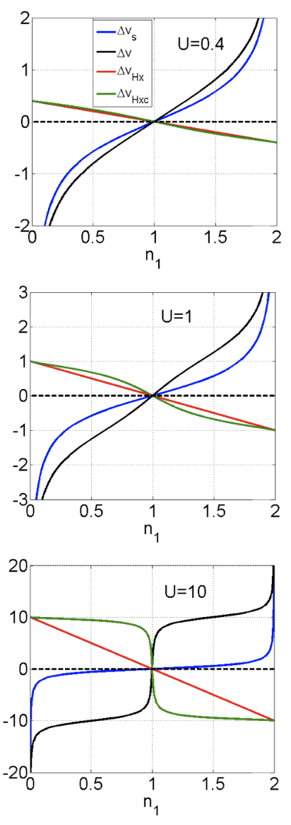
Figure 7: Plots of $\mathrm{\Delta}v_{\scriptscriptstyle\rm S}$ (blue) and its components, the one-body potential $\mathrm{\Delta}v$ (black), the Hartree plus exchange potentials, $U\mathrm{\Delta}n/2$ (red), and the same with correlation added, $U\mathrm{\Delta}n/2+\mathrm{\Delta}v_{\scriptscriptstyle\rm C}$ (green) plotted against $n_{1}$ for various values of $U$. Reproduced from Ref. Carrascal et al. (2015).

In Fig. 7, we show the contributions to the KS potential for a sequence of different $U$ values, as a function of the occupation. The effect of repulsion is to always oppose the potential difference, making the KS potential difference smaller. In the first, $U$ is small, and correlation is of order $U^{2}$ (see Reference Carrascal et al. (2015)). Thus the correlation contribution is negligible (red and green overlap) and HF is an excellent approximation. In the middle, $U=1$ is moderate, and now we begin to see the difference correlation makes in the potential. Moreover, its effect is to make $\mathrm{\Delta}v_{\scriptscriptstyle\rm HXC}$ deviate from a straight line. Finally, for strong correlation, the HXC potential (almost) exactly is equal and opposite to the one-body potential. Again, the HX contribution has much curvature, but now correlation wipes that out (almost) entirely. Clearly, the HF approximation will be terrible for the potential in this case, and yield entirely incorrect densities. In fact, a lower-energy solution appears if one allows spin symmetry breaking Perdew et al. (1995).

It is now relatively routine to calculate accurate KS potentials from highly accurate densities found, e.g., via quantum chemical methods Gaiduk et al. (2012). In an insanely demanding calculation, it is even possible to solve the KS equations using the exact XC functional Wagner et al. (2014). Convergence becomes more difficult as correlations grow stronger, but remains possible Wagner et al. (2013).

3.1 KS spectral function

There is a pernicious superstition Tacitus (109) that the KS spectrum is related to the physical response properties of the real system. This false belief has arisen because, for weakly correlated systems, this is approximately true, apart from the fundamental gap of a semiconductor. From a practical viewpoint, the KS bands are marvelously useful as a starting point for Green function calculations of real spectral functions. Moreover, long ago, when the local density approximation ruled supreme, there was no way to know if differences between the KS and exact response properties was due to the crudeness of this approximation Perdew et al. (1982); Sham and Schlüter (1983). These days, there are simple exact answers to such speculations, if we only have the patience to read them.

3.2 The ionization potential theorem

As a simple example of the mysterious workings of the exact functional, we state an important exact result

$$I(N)=E(N{-}1)-E(N)=-\varepsilon^{\rm HO}(N).$$ (18)

Here $E(N)$ is the ground-state of the $N$-electron system, and $\varepsilon^{\rm HO}$ is the energy of the highest-occupied KS orbital. (For those with some chemistry leaning, Koopmans’ theorem is an approximate version of this for HF calculations Parr and Yang (1989)). This illustrates some of the power of KS-DFT. You might think that, with the exact functional, all one can extract is the ground-state energy and density of our system. But the above result shows that the HO of the KS scheme also tells you the ionization energy. One can also extract all static response functions exactly by turning on weak external perturbations, and applying the exact functional to the perturbed systems. In practice, standard DFT approximations tend to violate this exact condition very badly Perdew et al. (1982); Sham and Schlüter (1983); Perdew and Levy (1983). Nonetheless, they often still yield usefully accurate ground-state energies, thus performing their primary function. (On the other hand, returning to the discussion of HKI, knowing the exact XC does not, in general, give you access to, say, the first excited state energy. It is a functional of $n_{1}$ alone, but we cannot deduce that functional from $E_{\scriptscriptstyle\rm XC}(n_{1})$.)

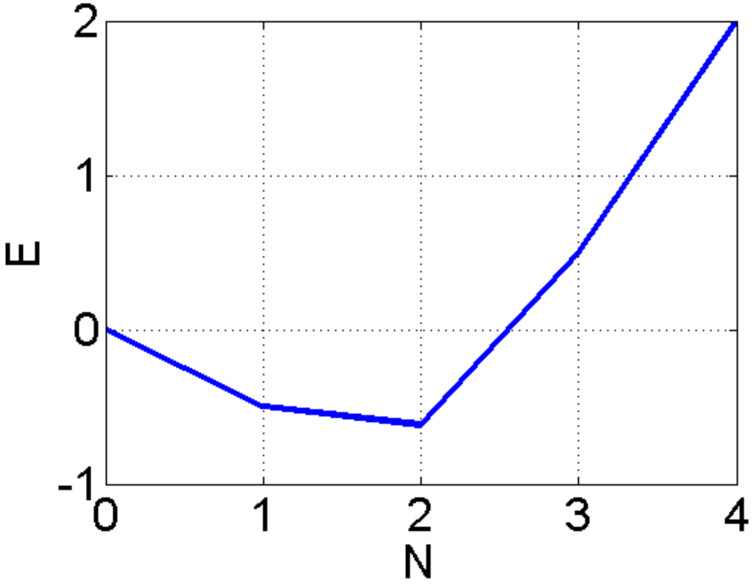
Figure 8: Plot of $E(N)$ for $U=1$ and $\mathrm{\Delta}v=0$. Reproduced from Ref. Carrascal et al. (2015).

Increasing $N$ by $1$ in Eq. (18) yields

$$A(N)=E(N)-E(N{+}1)=-\varepsilon^{\rm HO}(N{+}1)\neq\varepsilon^{\rm LU}(N),$$ (19)

where $A$ is called the electron affinity of the system in chemistry. The difference between the KS HO of the $N{+}1$ electron system and the lowest unoccupied (LU) level of the $N$-electron system is called $\mathrm{\Delta}_{\scriptscriptstyle\rm XC}$, where the $\mathrm{\Delta}$ indicates its origin from the infamous derivative discontinuity of DFT Perdew et al. (1982). This simply means, that at zero temperature, the energy of the system consists of straight line segments between integer values, as shown below in Fig. 8. The energy itself is continuous, but its derivative, the chemical potential, is not. For a neutral system, the chemical potential is $-I$ below the integer and $-A$ above. This discontinuous jump in $\mu$ shifts the KS HO eigenvalue by the same amount, producing the difference with the KS LU of the neutral. (Realistic electronic systems do not have an upward pointing portion of the curve in Fig. 8. This occurs for the dimer because electrons cannot escape to outside the system.)

3.3 Mind the gap

We are now ready to see the relevance of this to solids. Even for a finite system, we define the charge (or fundamental) gap as

$$E_{g}=I-A\,.$$ (20)

As the size of the system grows toward a bulk material, this quantity tends to the fundamental charge (or transport) gap of the system (at least for ordered systems Kohn (1964)). But, because of Eqs. (18) and (19) above, we find

$$E_{g}=E_{s,g}+\mathrm{\Delta}_{\scriptscriptstyle\rm XC}\,,$$ (21)

where$E_{s,g}$ is the KS gap (i.e., the difference between the LU and HO level, or the gap between the KS valence and conduction bands in a solid). Thus, with the exact XC functional of ground-state DFT, we do not get the true gap by looking at its KS value for the neutral system.

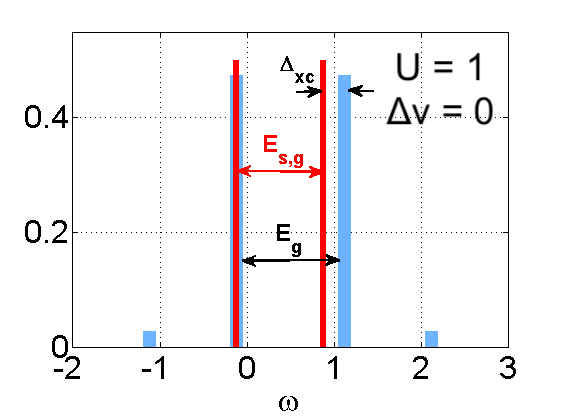
Figure 9: Spectral function of the symmetric dimer for $U=1$ and $\mathrm{\Delta}v=0$. The physical MB peaks are plotted in blue, the KS in red. Here $I=0.1$, $A=-1.1$, and $\varepsilon^{\rm LU}=0.9$. Reproduced from Ref. Carrascal et al. (2015).

Fig. 9 shows the spectral function (projected onto the left-hand site) in a weakly correlated case Carrascal et al. (2018), the symmetric dimer with $U=1$. We can see the sense in which the KS spectral function (red) resembles the blue exact one: the significant KS peaks are of about the same height and position as their blue counterparts, and the blue peaks without KS counterparts are relatively small. The KS gap is smaller than the true gap, but not by much. Because both the KS and the exact spectral functions satisfy the same sum rule (even with an approximate XC), if the dominant peaks are reproduced (even with the wrong gap), only small peaks are missed in the KS spectrum.

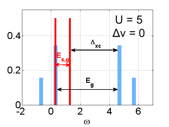
Figure 10: Same as Fig. 9, but now $U=5$. Here $I=-0.3$, $A=-4.7$, and $\varepsilon^{\rm LU}=1.3$. Note that the KS gap remains unchanged by the alteration of $U$ because $\mathrm{\Delta}n=0$ in both cases. Reproduced from Ref. Carrascal et al. (2015).

On the other hand, Fig. 10 shows the same system with a larger $U$ value. Now the strong KS peaks are not in the right place and are noticeably too large. Moreover, the blue peaks with no KS analogs are a substantial contribution.

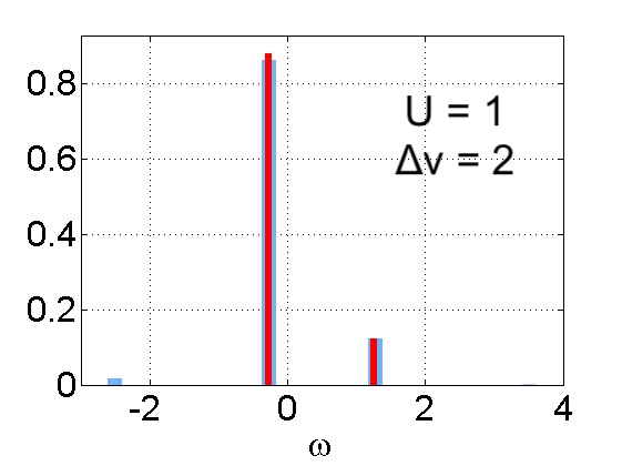
Figure 11: Same as Fig. 9, but now $U=1$, $\mathrm{\Delta}v=2$. Here $I=0.27$, $A=-1.27$, and $\varepsilon^{\rm LU}=1.25$. Reproduced from Ref. Carrascal et al. (2015).

Finally, in the inhomogeneous case, the potential asymmetry overcomes the effects of the Hubbard $U\!$. In Fig. 11, we see that for $\mathrm{\Delta}v=2$ and $U=1$, the KS spectral function is almost identical to the true one.

Lastly, we finish this section illustrating the relevance of this discussion to the thermodynamic limit. The canonical example of the Mott-Hubbard transition is a chain (or lattice) of H atoms. Each atom has one electron, so the bands of the KS potential are always half-filled, with no gap at the Fermi energy. Thus the gap is always zero and the KS band structure suggests it’s a metal. This may be true at moderate separations of the atoms, but as the separation is increased, the electrons must localize on atoms, and it must become a Mott insulator.

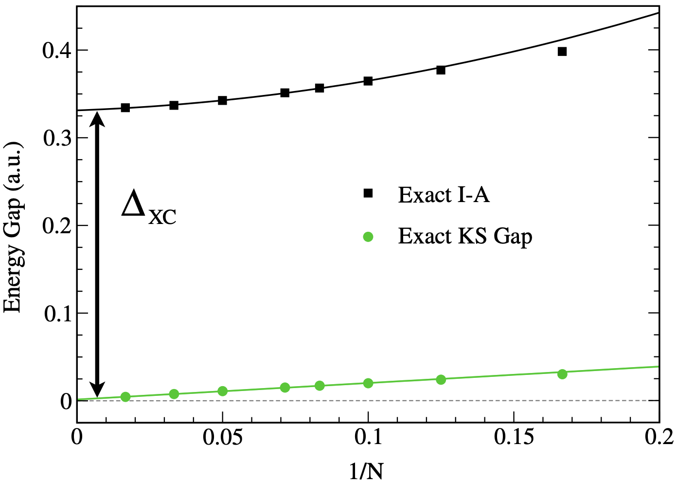
Figure 12: Exact gaps for chains of $N$ soft hydrogen atoms with atomic separation $b=4$ (error bars are less than symbol sizes). The upper curve is a quadratic fit of exact gaps of the largest six systems and extrapolates to a finite value $E_{g}\approx 0.33$. The exact Kohn-Sham gaps, in contrast, extrapolate to zero showing that for $N\rightarrow\infty$ the true KS system is metallic (lower curve is a linear fit of exact KS gaps of the largest six systems). Reproduced from Reference Stoudenmire et al. (2012).

Fig. 12 shows the gap, calculated for chains of well-separated 1D H atoms of increasing length Stoudenmire et al. (2012). By performing the calculation with finite systems, i.e., without periodic boundary conditions, we calculate the gap for each $N$ by adding and removing electrons, as in Eq. (20), and then take the limit as $N\to\infty$. On the other hand, we extract the exact ground-state density from our DMRG calculation at each $N\!$,  and find the corresponding exact KS potential for each $N\!$.  We could then as easily extrapolate the KS gap, from the HO and LU, showing that indeed the KS gap vanishes in the thermodynamic limit – exactly the same as if we had calculated the KS band structure, in which the Fermi energy would be right in the middle of the band. This provides a dramatic illustration of the KS underestimate of the true gap, even when using the exact XC functional.

3.4 Talking about ground-state DFT

First, we review our crucial formal points.

1. In general, the KS scheme with the exact functional yields ground-state energy and density, and any other quantities that can be teased from them, such as static response properties and ionization potentials.

2. There is no formal meaning for most KS eigenvalues in ground-state DFT, despite the fact that many practitioners treat them as if there were. Of course, they do provide tremendous physical and intuitive insight, especially for weakly correlated systems, where they are good approximations to the excitations (either quasi-particle or optical). But when correlations are strong, explicit methods are needed to correct them Zhang and Pavarini (2019).

3. The strongest manifestation of point 2 above is that the exact KS gap is typically smaller than the true gap, and can vanish in cases where the true gap is finite (Mott insulator).

4. Moreover, there is an exact formula relating the total energy to the sum of the KS eigenvalues, which contains finite corrections for double counting. There is no ambiguity about these corrections, they are derived from the formal theory, and yield the exact many-body energy. But when correlated methods are used for a subset of the orbitals, ambiguities can arise that affect occupancies Wang et al. (2012).

5. Although in principle, all properties are functionals of the ground-state density, knowledge of the exact ground-state energy functional (via $E_{\scriptscriptstyle\rm XC}$) does not provide a way to calculate these other functionals. As we see later, TDDFT is a way to do precisely this.

Next, we discuss how these points show up in practical DFT calculations of solids, where XC approximations must be made.

1. The steady progress within quantum chemistry and materials in functional development is almost entirely focused on improvements in accuracy and reliability of the total energy for weakly correlated systems Kohn et al. (1996); Mardirossian and Head-Gordon (2017). This is by far the most important use of DFT in modern electronic structure. Such improvements are often not particularly relevant to the response properties of greatest interest in strongly correlated materials. For example, the KS eigenvalues are often not improved significantly by functionals yielding better energies Stowasser and Hoffmann (1999); Tozer and Handy (1998). Although the KS eigenvalues cannot be directly interpreted in general, they are uniquely defined (up to a constant). Thus the exact KS Hamiltonian is a well-defined starting point for many-body methods.

2. The KS scheme is not a mean-field scheme in the traditional sense of the word, and it can be extremely difficult to relate its features to those of traditional many-body theory. The KS wavefunction is typically a single Slater determinant, but yields the exact many-body energy via its density.

3. Standard approximations, such as LDA and generalized gradient approximations (GGA), by construction produce total energies that are smooth and continuous at integer $N$, unlike the exact $E(N)$. Thus their corresponding $\mathrm{\Delta}_{\scriptscriptstyle\rm XC}$ is zeroPerdew et al. (1982). According to Sec. 3.3, the KS band gap in such approximations is their prediction for the fundamental gap. In fact, it has been found that their KS gaps are likely a good approximation to the exact KS gap Grüning et al. (2006), but their lack of discontinuous behavior means they miss the correction to turn it into the true gap.

4. On the other hand, the range-separated hybrid functional HSE06 is well-known to produce reasonable gaps for moderate gap semiconductors. This is because, instead of performing a true pure KS calculation, most codes (like VASP) perform a generalized KS calculation Seidl et al. (1996) when a functional is orbital-dependentHafner (2008); Perdew et al. (2017). They treat the orbital-dependent part of the potential as if it were a many-body potential, just as is done in HF. (A similar but smaller effect occurs in meta-GGA’s that depend on the kinetic energy density, such as SCAN Sun et al. (2016)). And in fact clever tricks may be used to extract the true gap, even from a periodic code Görling (2015).

4 Time-dependent DFT (TDDFT)

Our last main section is about time-dependent density functional theory (TDDFT) Burke et al. (2005); Marques et al. (2012); Ullrich (2012); Maitra (2016). While this uses many of the forms and conventions of ground-state DFT, it is in fact based on a very different theorem from the HK theorems. When applied to the linear response of a system to a dynamic electric field, it yields the optical transitions (and oscillator strengths) of that system. It has become the standard method for extracting low-level excitations in molecules, where traditional quantum chemical calculations are even more demanding than those for the ground state.

The Runge-Gross theorem Runge and Gross (1984) states that, for a given initial wavefunction, statistics, and interaction, the time-dependent density uniquely determines the one-body potential. In principle, this can be used for any many-electron time-dependent problem, including those in strong laser fields Burke et al. (2005). In practice, such calculations are limited by the accuracy of the approximations and whether the observable of interest can be extracted directly from the one-electron density. One constructs TD KS equations, defined to yield the exact time-dependent one-electron density. Because TDDFT applies to the time-dependent Schrödinger equation, the XC functional differs from that of ground-state DFT in general, and has a time-dependence.

Our interest will be only in the linear-response regime. In that case, one can derive a crucial result, which we give in operator form, called the Gross-Kohn equation Gross and Kohn (1985)

$$\chi(\omega)=\chi_{\scriptscriptstyle\rm S}(\omega)+\chi_{\scriptscriptstyle\rm S}(\omega)*(f_{\scriptscriptstyle\rm H}+f_{\scriptscriptstyle\rm XC}(\omega))*\chi(\omega),$$ (22)

where $\chi(\omega)$ is the dynamic density-density response function of the system, and $\chi_{\scriptscriptstyle\rm S}$ is its KS counterpart. The kernel, $f\!$,  is the functional derivative of the time-dependent potential. Thus, $f_{\scriptscriptstyle\rm H}$ is the Hartree contribution, while $f_{\scriptscriptstyle\rm XC}(\omega)$ is the XC correction.

Eq. (22) is a Dyson-like equation for the polarization. If we set $f_{\scriptscriptstyle\rm XC}=0$, it is the standard random-phase approximation, the Coulomb interaction simply dressing the bare interaction, and producing all the bubble diagrams. But things get a little weird when we assert that inclusion of $f_{\scriptscriptstyle\rm XC}(\omega)$ produces the exact response of the system, for all frequencies. From a many-body viewpoint, this is suspicious, as these are a closed set of equations without coupling to 4-point functions. But the logic is sound and exactly analogous to the ground-state: there exists such a function that could be considered as defined by Eq. (22).

The excitations of a system are given by poles of its response function. Simple analysis (exactly that of RPA) yields a matrix equation that corrects KS transition frequencies to the true transition frequencies, where the matrix elements involve $f_{\scriptscriptstyle\rm H}+f_{\scriptscriptstyle\rm XC}$. With standard ground-state approximations, folks have merrily calculated mostly low-lying valence transitions from the ground-state of many molecules Adamo and Jacquemin (2013), finding accuracies a little lower than those of ground-state DFT Jacquemin et al. (2009), and computational costs that are comparable. This has been invaluable for larger molecules, where many excitations of the same symmetry may overlap, and so TDDFT yields a semiquantitative signature that can be easily matched with experiment Bauernschmitt et al. (1998).

However, not all is well in paradise. Almost immediately, it was noticed that the use of a ground-state approximation is simply the static limit of the corresponding kernel, and can be easily shown to produce only single excitations. While useful workarounds were created for some cases, it was also found that going to higher-order response does not solve the problem. And many of the most exciting transitions in biochemistry are double excitations.

4.1 Hubbard dimer

Happily we care only about Hubbard dimers, where everything is much simpler. First, we note our Hubbard dimer, in the singlet space, has just three states: the ground-state, the first excited state, which has a single excitation, and the second excited state, which is a double excitation out of the ground-state. Since there are no spatial degrees of freedom, our $\chi(\omega)$ is the Fourier transform of $\mathrm{\Delta}n(t)/\mathrm{\Delta}v(0)$, which is just a scalar, with $\omega$-dependence

$$\chi_{n}(\omega)=\frac{a_{1}}{\omega^{2}-\omega_{1}^{2}}+\frac{a_{2}}{\omega^{2}-\omega_{2}^{2}},$$ (23)

where $\omega_{i}$ denotes the transition frequency and $a_{i}$ is related to its oscillator strength Carrascal et al. (2018). Thus $\chi$ has poles at each of the transition frequencies. Fig. 13 shows the value of each of these transitions as a function of $\mathrm{\Delta}v$ for $U=1$. The double excitation is a little above the single for the symmetric case, but grows linearly with $\mathrm{\Delta}v$. The single remains about the same, and even dips, until $\mathrm{\Delta}v=U\!$,  and then begins to grow itself. Here we can use our model system to examine one of the key mysteries of practical TDDFT: Where did all the higher excitations go?

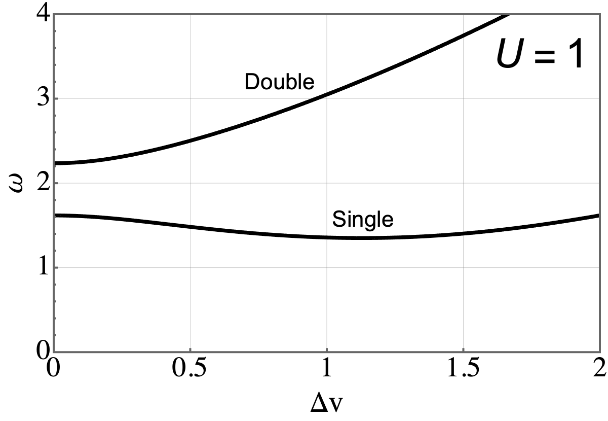
Figure 13: Transition frequencies of the first and second excitations as a function of $\Delta v$ for $U=1$.

First we do an exact ground-state KS calculation, as in the previous sections. Thus the exact KS system is a tight-binding problem with effective potential, $\mathrm{\Delta}v_{\scriptscriptstyle\rm S}$, defined to yield the exact ground state $\mathrm{\Delta}n$. This yields two eigenvalues, the lower symmetric combination and the higher asymmetric combination. The KS ground-state has the lower one doubly occupied. There do exist KS analogs of the many-body states. The single excitation has one electron excited to the higher level, the double has both. Fig. 14 adds the KS transitions to Fig. 13, showing that they loosely follow the accurate transitions, but are significantly different.

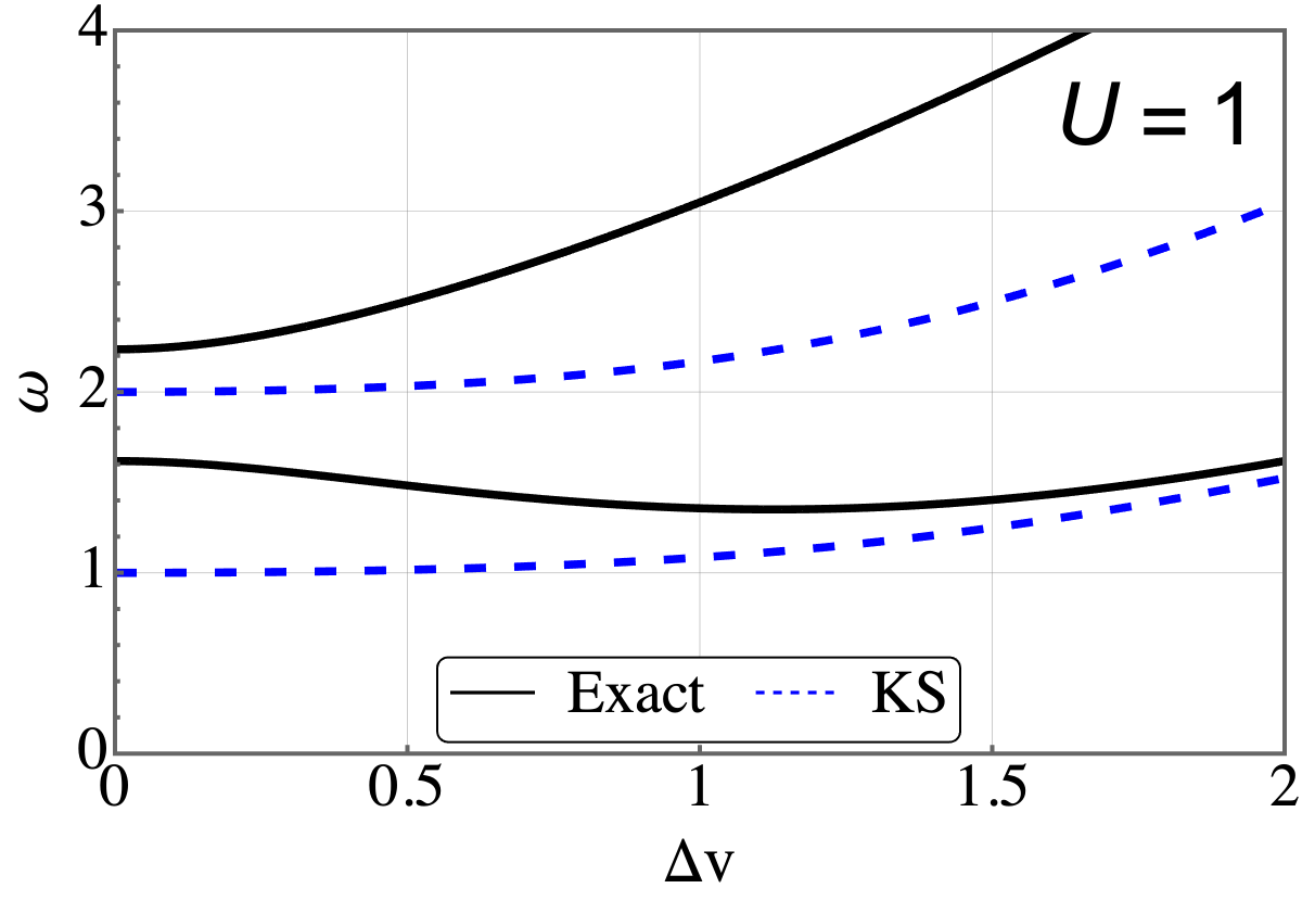
Figure 14: Same as Fig. 13, but with KS transitions (depicted in blue). For $\mathrm{\Delta}v>U\!$, the KS transition is a very good approximation to the true transition.

In the KS response function, $\chi_{\scriptscriptstyle\rm S}$, the matrix elements of the density operator between ground and double excitation are zero, since both KS orbitals are different, so the Slater determinants are not coupled by a single density operator. Hence, such states have no numerator, eliminating any poles that might have arisen in the denominator, i.e.,

$$\chi_{\scriptscriptstyle\rm S}(\omega)=\frac{a_{s}}{\omega^{2}-\omega_{s}^{2}}\,.$$ (24)

Thus the second KS transition, the double, does not appear at all in the response function! It’s position is correctly marked in Fig. 14, but cannot be seen in $\chi_{\scriptscriptstyle\rm S}$.

By requiring the poles occur at the right places, one finds (in general) a matrix equation in the space of single excitations for the true transitions, whose elements are determined by the kernel. Here, this is one dimensional, yielding

$$\omega^{2}=\omega_{\scriptscriptstyle\rm S}^{2}+2\omega_{\scriptscriptstyle\rm S}\,f_{\scriptscriptstyle\rm HXC}(\omega)\,\frac{2}{1+\mathrm{\Delta}v_{\scriptscriptstyle\rm S}^{2}}\,.$$ (25)

The adiabatically exact approximation (AE) is to use the exact ground-state functional here to calculate $f_{\scriptscriptstyle\rm HXC}$. This corrects the single KS transition and is shown in Fig. 15. This works extremely well to capture almost all the difference with the KS transition, yielding very accurate excitations. This becomes even better for $\mathrm{\Delta}v$ greater than $U$, where the corrections virtually vanish (just as in Fig. 11 for the spectral function).

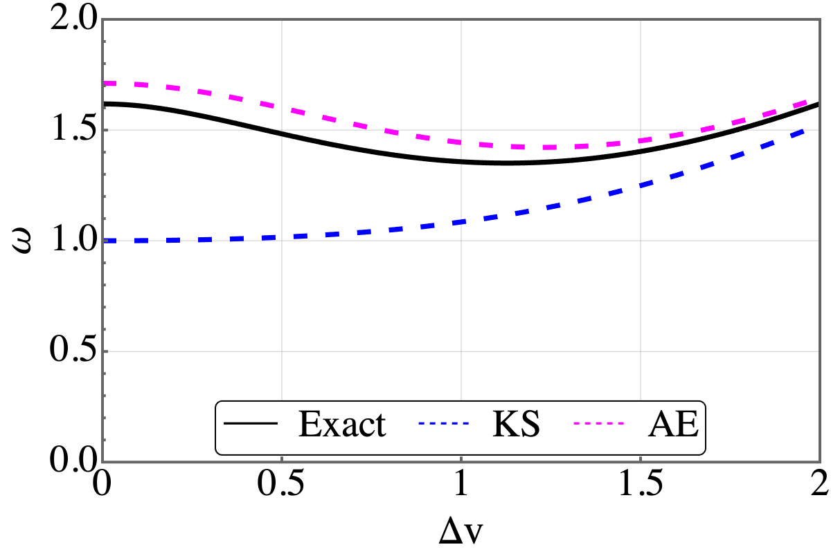
Figure 15: Same as Fig. 13, but with the adiabatically exact approximation (AE, pink dashes).

But Eq. (25) just has one solution if the $\omega$-dependence in the kernel is neglected. On the other hand, if there is strong frequency dependence in the kernel, new transitions, not in the KS system, may appear. In fact, we know that is precisely what happens, as the physical system does have a double excitation. To understand how standard TDDFT fails, we note that we can calculate the exact kernel by finding $\chi(\omega)$ from many-body calculations, $\chi_{\scriptscriptstyle\rm S}(\omega)$ by the techniques of the earlier section, inverting and subtracting

$$f_{\scriptscriptstyle\rm HXC}(\omega)=\chi_{\scriptscriptstyle\rm S}^{-1}(\omega)-\chi^{-1}(\omega)\,.$$ (26)

Fig. 16 shows the singular frequency-dependence of the kernel from Eq. (26), which allows Eq. (25) to have an additional solution.

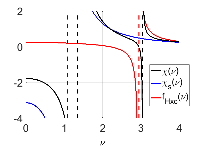
Figure 16: Frequency dependence of exact (black) and Kohn-Sham susceptibilities (blue) and exchange-correlation kernel (red) for $U=\mathrm{\Delta}v=1$. Poles marked by dashed vertical lines, as a function of frequency $\nu$. The red line shows the exchange-correlation kernel. Reproduced from Ref. Carrascal et al. (2018).

However, while all this provides insight into how the exact functional performs its magic, it does not tell us directly how to create a general purpose model, which would build this frequency-dependence into an explicit density functional sufficiently accurately to capture double excitations Maitra (2016).

4.2 Talking about TDDFT

We saw in the earlier sections how the KS eigenvalues did not have a formal meaning in pure ground-state KS-DFT. We have seen here that, with the advent of TDDFT, they form the starting point of a scheme which produces the optical excitations. These are not the quasi-particle excitations associated with the Green function, which involve a change in particle number.

While the primary function of approximate ground-state DFT is to find energies, it usually also produces reasonably accurate densities, but rather erroneous XC potentials. In fact, this feat is achieved by having all the occupied orbitals shifted (higher) than their exact KS counterparts. A constant shift has no effect on the density. But if the unoccupied levels (at least, the low-lying valence excitations) suffer the same shift, then KS transition frequencies are unaffected, and the adiabatic approximation (usually applied to the same XC approximation as the ground-state calculation) is reasonably accurate for many weakly correlated molecules.

Linear-response TDDFT has been less used in solids, because in the case of insulators, it became clear early on Onida et al. (2002) that there is a long-range contribution to the XC kernel (as long-ranged as the Hartree contribution is) that is missed when using a semilocal ground-state approximation adiabatically. There are now many ways around this difficulty Sharma et al. (2011), some based on modelling the kernel using many-body techniques.

There have been many other approaches suggested for extracting optical excitations from DFT. An old simple one is called $\mathrm{\Delta}$-SCF Ziegler et al. (1977), which involves simply using excited-state occupation numbers in a KS calculation, and finding the energy the usual way. Another, which has seen considerable recent interest Gould and Pittalis (2019); Yang et al. (2017), is to use ensemble DFT Gross et al. (1988).

5 Summary

This short review is aimed at broadening understanding of the basic differences between a density functional viewpoint and that of traditional many-body theory. The emphasis here has been on the exact theory, which we have illustrated on the 2-site Hubbard model. We have shown it is confusing to consider KS theory as any kind of traditional mean-field theory, and how the addition of TDDFT allows one to consider the KS eigenvalues as zero-order approximations to the optical excitations, not the quasiparticle excitations.

However, the only reason that anyone cares about the exact theory of DFT is because, in practice, it is extremely useful with relatively unsophisticated approximations. These begin with the famous local density approximation, in which the XC energy per electron at each point in a system is approximated by that of a uniform gas matching the density at this point. This was introduced already in the KS paper (where the statement of exactness appears as a mere footnote), thereby totally muddying the waters between exact and approximate statements. Walter Kohn told KB that he simply noticed the exact nature of the KS scheme after submitting the paper. From about 1990 onwards, many users began using more sophisticated functionals, whose primary effect was to improve total energies and energy differences.

This article has said little or nothing about how to understand such approximations. This is because local (and semilocal) approximations capture a universal limit of all electronic systems, by yielding relatively exact XC energies in this limit Lieb and Simon (1973); Elliott and Burke (2009); Cancio et al. (2018); Okun and Burke (2021). Traditional many-body theory generally considers a power series expansion in the electron-electron interaction. The alternative limit simultaneously increases the number of particles, in a way that the total electron-electron repulsion remains a finite fraction of the total energy even as interactions become weaker. The simplest example of this is that the LDA for exchange, whose formula can be derived by hand, has a percentage error that vanishes for atoms as $Z=N\to\infty$ Elliott and Burke (2009).

This limit is hard-wired into the last term of the real-space Hamiltonian of Eq. (1), which is the integral of the density times the one-body potential. This is why the density is the basic variable in DFT. Even if formal theorems can be proven using other variables, this is why density functional theory has been so successful. It is also the case that the one-body potentials to which we apply DFT are diagonal in coordinate space, which is related to why the LDA is a universal limit.

Thus, key aspects of DFT approximations that are crucial to its success are missing from lattice models like the Hubbard model. There is no corresponding universal limit in which LDA becomes exact, even if one uses an approximation based on the uniform case Lima et al. (2002); Franca et al. (2011). Again, this is why we created our 1D real-space mimic of 3D reality, instead of just solving lattice models.

6 Acknowledgments

K.B. acknowledges support from the Department of Energy, Award No. DOE DE-SC0008696. J.K. acknowledges support from the Department of Energy, Award No. DE-FG02-08ER46496. We thank Eva Pavarini for suggesting this chapter, and making us write it.

Appendix A Exercises

If you have followed the logic throughout this tutorial, you will enjoy sorting out these little questions. If you want solutions, please email either of the authors, with a brief note about your current status and interests.

1. State which aspect of Fig. 4 illustrates the HKI theorem.

2. What geometrical construction gives you the corresponding ground-state potential for a given $n_{1}$ in Fig. 5?

3. Study the extreme edges ($n_{1}=0$ and $2$) of Fig. 5. What interesting qualitative feature is barely visible, and why must it be there?

4. What feature must always be present in Fig. 5 near $n_{1}=1$? Explain.

5. How can you be sure that, no matter how large $U$ becomes, $F_{\scriptscriptstyle\rm U}(n_{1})$ is never quite $U|1{-}n_{1}|$?

6. Assuming the blue line is essentially that of $U=0$, use geometry on Fig. 3 to find $\mathrm{\Delta}v_{\scriptscriptstyle\rm S}$ for $U=5$.

7. What is the relation, if any, between each of the blue plots in the three panels of Fig. 7? Explain.

8. What is the relation, if any, between each of the red plots in the three panels of Fig. 7? Explain.

9. Why is the green line almost the mirror image of the black line in the $U=10$ panel of Fig. 7? Could it be the exact mirror image? Explain.

10. From Fig. 8, using $E(N)$ about $N{\;=\;}2$, determine the locations of the largest peaks of Fig. 9 and compute the gap between them.

11. Sketch how Fig. 8 must look if $U=10$ and $\mathrm{\Delta}v=0$.

12. What is the relation between the two blue lines in Fig. 14? Explain.

13. Give a rule relating the numbers of vertical lines of different color in Fig. 16.
    Explain its significance.

14. Recall the definition of the kernel from section 4. Using this, derive $f_{\scriptscriptstyle\rm H}$ and $f_{\scriptscriptstyle\rm X}$, and draw them on Fig. 16. Explain where double excitations must come from for 2 electrons.

15. Using formulas and figures from both sections, deduce the results of Fig. 15 in the absence of correlation (Hint: You will need to solve the Hartree-Fock self-consistent equations), and comment on the relative errors. This is a little more work than the other exercises.

References

- Mahan (2000) G. D. Mahan, Many-Particle Physics (Springer, 3rd edition, New York, 2000).
- Blöchl (2011) Peter Blöchl, “Theory and practice of density-functional theory,” in Pavarini et al. (2011).
- Pribram-Jones et al. (2015) Aurora Pribram-Jones, David A. Gross, and Kieron Burke, “DFT: A theory full of holes?” Annual Review of Physical Chemistry 66, 283–304 (2015).
- Pickard et al. (2020) Chris J. Pickard, Ion Errea, and Mikhail I. Eremets, “Superconducting hydrides under pressure,” Annual Review of Condensed Matter Physics 11, 57–76 (2020).
- Nørskov et al. (2011) Jens K. Nørskov, Frank Abild-Pedersen, Felix Studt, and Thomas Bligaard, “Density functional theory in surface chemistry and catalysis,” Proceedings of the National Academy of Sciences 108, 937 (2011).
- Zeng et al. (2019) Li Zeng, Stein B. Jacobsen, Dimitar D. Sasselov, Michail I. Petaev, Andrew Vanderburg, Mercedes Lopez-Morales, Juan Perez-Mercader, Thomas R. Mattsson, Gongjie Li, Matthew Z. Heising, Aldo S. Bonomo, Mario Damasso, Travis A. Berger, Hao Cao, Amit Levi, and Robin D. Wordsworth, “Growth model interpretation of planet size distribution,” Proceedings of the National Academy of Sciences 116, 9723–9728 (2019).
- Velez et al. (2019) Zélia Velez, Christina C. Roggatz, David M. Benoit, Jörg D. Hardege, and Peter C. Hubbard, “Short- and medium-term exposure to ocean acidification reduces olfactory sensitivity in gilthead seabream,” Frontiers in Physiology 10, 731 (2019).
- Hendon et al. (2014) Christopher H. Hendon, Lesley Colonna-Dashwood, and Maxwell Colonna-Dashwood, “The role of dissolved cations in coffee extraction,” Journal of Agricultural and Food Chemistry, Journal of Agricultural and Food Chemistry 62, 4947–4950 (2014).
- Lechermann (2011) Frank Lechermann, “Model hamiltonians and basic techniques,” in Pavarini et al. (2011).
- Solovyev (2008) I V Solovyev, “Combining DFT and many-body methods to understand correlated materials,” Journal of Physics: Condensed Matter 20, 293201 (2008).
- Tsui et al. (1982) D. C. Tsui, H. L. Stormer, and A. C. Gossard, “Two-dimensional magnetotransport in the extreme quantum limit,” Phys. Rev. Lett. 48, 1559–1562 (1982).
- Kondo (1964) Jun Kondo, “Resistance Minimum in Dilute Magnetic Alloys,” Progress of Theoretical Physics 32, 37–49 (1964).
- Lieb (1983) Elliott H. Lieb, “Density functionals for coulomb systems,” Int. J. Quantum Chem. 24, 243–277 (1983).
- Loewen (2008) J. Loewen, Lies My Teacher Told Me: Everything Your American History Textbook Got Wrong (New Press, 2008).
- Haldane (2017) F. Duncan M. Haldane, “Nobel lecture: Topological quantum matter,” Rev. Mod. Phys. 89, 040502 (2017).
- Lee and Scuseria (1995) Timothy J. Lee and Gustavo E. Scuseria, “Achieving chemical accuracy with coupled-cluster theory,” in Quantum Mechanical Electronic Structure Calculations with Chemical Accuracy, edited by Stephen R. Langhoff (Springer Netherlands, Dordrecht, 1995) pp. 47–108.
- Feller and Peterson (2007) David Feller and Kirk A. Peterson, “Probing the limits of accuracy in electronic structure calculations: Is theory capable of results uniformly better than “chemical accuracy”?” The Journal of Chemical Physics 126, 114105 (2007).
- Vuckovic et al. (2019) Stefan Vuckovic, Suhwan Song, John Kozlowski, Eunji Sim, and Kieron Burke, “Density functional analysis: The theory of density-corrected DFT,” Journal of Chemical Theory and Computation 15, 6636–6646 (2019).
- Hafner et al. (2011) Jürgen Hafner, Christopher Wolverton, and Gerbrand Ceder, “Toward Computational Materials Design: The Impact of Density Functional Theory on Materials Research,” MRS Bulletin 31, 659–668 (2011).
- O’Regan and Grätzel (1991) Brian O’Regan and Michael Grätzel, “A low-cost, high-efficiency solar cell based on dye-sensitized colloidal tio2 films,” Nature 353, 737–740 (1991).
- Burke and Wagner (2013) Kieron Burke and Lucas O. Wagner, “DFT in a nutshell,” International Journal of Quantum Chemistry, International Journal of Quantum Chemistry 113, 96–101 (2013).
- Burke (2007) K Burke, The ABC of DFT (2007).
- Dreizler and Gross (1989) R.M. Dreizler and E.K.U. Gross, Density Functional Theory: An Approach to the Quantum Many-Body Problem (Springer Berlin Heidelberg, 1989).
- (24) Centre Européen de Calcul Atomique et Moléculaire, “Teaching the theory in density functional theory,” .
- Carrascal et al. (2015) D J Carrascal, J Ferrer, J C Smith, and K Burke, “The hubbard dimer: a density functional case study of a many-body problem,” Journal of Physics: Condensed Matter 27, 393001 (2015).
- Carrascal et al. (2018) Diego J. Carrascal, Jaime Ferrer, Neepa Maitra, and Kieron Burke, “Linear response time-dependent density functional theory of the hubbard dimer,” The European Physical Journal B 91, 142 (2018).
- Ullrich (2018) Carsten A. Ullrich, “Density-functional theory for systems with noncollinear spin: Orbital-dependent exchange-correlation functionals and their application to the hubbard dimer,” Phys. Rev. B 98, 035140 (2018).
- Sagredo and Burke (2018) Francisca Sagredo and Kieron Burke, “Accurate double excitations from ensemble density functional calculations,” The Journal of Chemical Physics 149, 134103 (2018).
- Sagredo and Burke (2020) Francisca Sagredo and Kieron Burke, “Confirmation of the pplb derivative discontinuity: Exact chemical potential at finite temperatures of a model system,” Journal of Chemical Theory and Computation, Journal of Chemical Theory and Computation 16, 7225–7231 (2020).
- Szabo and Ostlund (1996) A. Szabo and N. S. Ostlund, Modern Quantum Chemistry (Dover Publishing, Mineola, New York, 1996).
- Ochterski et al. (1995) Joseph W. Ochterski, George A. Petersson, and Kenneth B. Wiberg, “A comparison of model chemistries,” Journal of the American Chemical Society, Journal of the American Chemical Society 117, 11299–11308 (1995).
- Bartlett and Musial (2007) Rodney J. Bartlett and Monika Musial, “Coupled-cluster theory in quantum chemistry,” Rev. Mod. Phys. 79, 291–352 (2007).
- Girvin and Yang (2019) S.M. Girvin and K. Yang, Modern Condensed Matter Physics (Cambridge University Press, 2019).
- Cohen et al. (2008) Aron J. Cohen, Paula Mori-Sánchez, and Weitao Yang, “Insights into current limitations of density functional theory,” Science 321, 792–794 (2008).
- Jacob et al. (2020) David Jacob, Gianluca Stefanucci, and Stefan Kurth, “Mott metal-insulator transition from steady-state density functional theory,” Phys. Rev. Lett. 125, 216401 (2020).
- Himmetoglu et al. (2014) Burak Himmetoglu, Andrea Floris, Stefano de Gironcoli, and Matteo Cococcioni, “Hubbard-corrected DFT energy functionals: The LDA+U description of correlated systems,” International Journal of Quantum Chemistry 114, 14–49 (2014).
- Anisimov et al. (1997) V I Anisimov, A I Poteryaev, M A Korotin, A O Anokhin, and G Kotliar, “First-principles calculations of the electronic structure and spectra of strongly correlated systems: dynamical mean-field theory,” Journal of Physics: Condensed Matter 9, 7359 (1997).
- Kotliar et al. (2006) G. Kotliar, S. Y. Savrasov, K. Haule, V. S. Oudovenko, O. Parcollet, and C. A. Marianetti, “Electronic structure calculations with dynamical mean-field theory,” Rev. Mod. Phys. 78, 865–951 (2006).
- Vollhardt (2011) Dieter Vollhardt, “Dynamical mean-field approach for strongly correlated materials,” in Pavarini et al. (2011).
- Pavarini (2011) Eva Pavarini, “The LDA+DMFT approach,” in Pavarini et al. (2011).
- Wilde (1887) O. Wilde, The Canterville Ghost (1887).
- Harriman (1986) John E. Harriman, “Densities, operators, and basis sets,” Phys. Rev. A 34, 29–39 (1986).
- LeBlanc et al. (2015) J. P. F. LeBlanc, Andrey E. Antipov, Federico Becca, Ireneusz W. Bulik, Garnet Kin-Lic Chan, Chia-Min Chung, Youjin Deng, Michel Ferrero, Thomas M. Henderson, Carlos A. Jiménez-Hoyos, E. Kozik, Xuan-Wen Liu, Andrew J. Millis, N. V. Prokof’ev, Mingpu Qin, Gustavo E. Scuseria, Hao Shi, B. V. Svistunov, Luca F. Tocchio, I. S. Tupitsyn, Steven R. White, Shiwei Zhang, Bo-Xiao Zheng, Zhenyue Zhu, and Emanuel Gull (Simons Collaboration on the Many-Electron Problem), “Solutions of the two-dimensional hubbard model: Benchmarks and results from a wide range of numerical algorithms,” Phys. Rev. X 5, 041041 (2015).
- Yang et al. (2014) Jun Yang, Weifeng Hu, Denis Usvyat, Devin Matthews, Martin Schütz, and Garnet Kin-Lic Chan, “Ab initio determination of the crystalline benzene lattice energy to sub-kilojoule/mole accuracy,” Science 345, 640–643 (2014).
- Lejaeghere et al. (2016) Kurt Lejaeghere et al., “Reproducibility in density functional theory calculations of solids,” Science 351 (2016).
- Stoudenmire et al. (2012) E. M. Stoudenmire, Lucas O. Wagner, Steven R. White, and Kieron Burke, “One-dimensional continuum electronic structure with the density-matrix renormalization group and its implications for density-functional theory,” Phys. Rev. Lett. 109, 056402 (2012).
- Baker et al. (2015) Thomas E. Baker, E. Miles Stoudenmire, Lucas O. Wagner, Kieron Burke, and Steven R. White, “One-dimensional mimicking of electronic structure: The case for exponentials,” Phys. Rev. B 91, 235141 (2015).
- White (1992) Steven R. White, “Density matrix formulation for quantum renormalization groups,” Phys. Rev. Lett. 69, 2863–2866 (1992).
- White (1993) Steven R. White, “Density-matrix algorithms for quantum renormalization groups,” Phys. Rev. B 48, 10345–10356 (1993).
- Kohn and Sham (1965) W. Kohn and L. J. Sham, “Self-consistent equations including exchange and correlation effects,” Phys. Rev. 140, A1133–A1138 (1965).
- Wagner et al. (2012) Lucas O. Wagner, E. M. Stoudenmire, Kieron Burke, and Steven R. White, “Reference electronic structure calculations in one dimension,” Phys. Chem. Chem. Phys. 14, 8581–8590 (2012).
- Hubbard (1963) J. Hubbard, “Electron correlations in narrow energy bands,” Proceedings of the Royal Society of London. Series A. Mathematical and Physical Sciences 276, 238–257 (1963).
- Hohenberg and Kohn (1964) P. Hohenberg and W. Kohn, “Inhomogeneous electron gas,” Phys. Rev. 136, B864–B871 (1964).
- Levy (1982) Mel Levy, “Electron densities in search of hamiltonians,” Phys. Rev. A 26, 1200–1208 (1982).
- Moreno et al. (2020) Javier Robledo Moreno, Giuseppe Carleo, and Antoine Georges, “Deep learning the hohenberg-kohn maps of density functional theory,” Phys. Rev. Lett. 125, 076402 (2020).
- Moreno et al. (2021) Javier Robledo Moreno, Johannes Flick, and Antoine Georges, “Machine learning band gaps from the electron density,” (2021), arXiv:2104.14351 [cond-mat.dis-nn] .
- Levy (1979) Mel Levy, “Universal variational functionals of electron densities, first-order density matrices, and natural spin-orbitals and solution of the -representability problem,” Proceedings of the National Academy of Sciences of the United States of America 76, 6062–6065 (1979).
- Thomas (1927) L. H. Thomas, “The calculation of atomic fields,” Math. Proc. Camb. Phil. Soc. 23, 542–548 (1927).
- Fermi (1928) E. Fermi, “Eine statistische Methode zur Bestimmung einiger Eigenschaften des Atoms und ihre Anwendung auf die Theorie des periodischen Systems der Elemente (a statistical method for the determination of some atomic properties and the application of this method to the theory of the periodic system of elements),” Zeitschrift für Physik A Hadrons and Nuclei 48, 73–79 (1928).
- Burke (2012) Kieron Burke, “Perspective on density functional theory,” The Journal of Chemical Physics 136, 150901 (2012).
- Dirac (1930) P. A. M. Dirac, “Note on exchange phenomena in the Thomas atom,” Mathematical Proceedings of the Cambridge Philosophical Society 26, 376–385 (1930).
- Umrigar and Gonze (1994) C. J. Umrigar and Xavier Gonze, “Accurate exchange-correlation potentials and total-energy components for the helium isoelectronic series,” Phys. Rev. A 50, 3827–3837 (1994).
- Perdew and Zunger (1981) J. P. Perdew and Alex Zunger, “Self-interaction correction to density-functional approximations for many-electron systems,” Phys. Rev. B 23, 5048–5079 (1981).
- Perdew et al. (1995) John P. Perdew, Andreas Savin, and Kieron Burke, “Escaping the symmetry dilemma through a pair-density interpretation of spin-density functional theory,” Phys. Rev. A 51, 4531–4541 (1995).
- Gaiduk et al. (2012) Alex P. Gaiduk, Dzmitry S. Firaha, and Viktor N. Staroverov, “Improved electronic excitation energies from shape-corrected semilocal kohn-sham potentials,” Phys. Rev. Lett. 108, 253005 (2012).
- Wagner et al. (2014) Lucas O. Wagner, Thomas E. Baker, M. Stoudenmire, E., Kieron Burke, and Steven R. White, “Kohn-sham calculations with the exact functional,” Phys. Rev. B 90, 045109 (2014).
- Wagner et al. (2013) Lucas O. Wagner, E. M. Stoudenmire, Kieron Burke, and Steven R. White, “Guaranteed convergence of the kohn-sham equations,” Phys. Rev. Lett. 111, 093003 (2013).
- Tacitus (109) P. C. Tacitus, Annals 15.44 (109).
- Perdew et al. (1982) John P. Perdew, Robert G. Parr, Mel Levy, and Jose L. Balduz, “Density-functional theory for fractional particle number: Derivative discontinuities of the energy,” Phys. Rev. Lett. 49, 1691–1694 (1982).
- Sham and Schlüter (1983) L. J. Sham and M. Schlüter, “Density-functional theory of the energy gap,” Phys. Rev. Lett. 51, 1888–1891 (1983).
- Parr and Yang (1989) R. G. Parr and W. Yang, Density Functional Theory of Atoms and Molecules (Oxford University Press, 1989).
- Perdew and Levy (1983) John P. Perdew and Mel Levy, “Physical content of the exact kohn-sham orbital energies: Band gaps and derivative discontinuities,” Phys. Rev. Lett. 51, 1884–1887 (1983).
- Kohn (1964) Walter Kohn, “Theory of the insulating state,” Phys. Rev. 133, A171–A181 (1964).
- Zhang and Pavarini (2019) Guoren Zhang and Eva Pavarini, “Optical conductivity, fermi surface, and spin-orbit coupling effects in ,” Phys. Rev. B 99, 125102 (2019).
- Wang et al. (2012) Xin Wang, M. J. Han, Luca de’ Medici, Hyowon Park, C. A. Marianetti, and Andrew J. Millis, “Covalency, double-counting, and the metal-insulator phase diagram in transition metal oxides,” Phys. Rev. B 86, 195136 (2012).
- Kohn et al. (1996) W. Kohn, A. Becke, and R. G. Parr, “Density functional theory of electronic structure,” J. Phys. Chem. 100, 12974 (1996).
- Mardirossian and Head-Gordon (2017) Narbe Mardirossian and Martin Head-Gordon, “Thirty years of density functional theory in computational chemistry: an overview and extensive assessment of 200 density functionals,” Molecular Physics 115, 2315–2372 (2017).
- Stowasser and Hoffmann (1999) Ralf Stowasser and Roald Hoffmann, “What do the kohn-sham orbitals and eigenvalues mean?” Journal of the American Chemical Society, Journal of the American Chemical Society 121, 3414–3420 (1999).
- Tozer and Handy (1998) David J. Tozer and Nicholas C. Handy, “Improving virtual kohn–sham orbitals and eigenvalues: Application to excitation energies and static polarizabilities,” The Journal of Chemical Physics, The Journal of Chemical Physics 109, 10180–10189 (1998).
- Grüning et al. (2006) Myrta Grüning, Andrea Marini, and Angel Rubio, “Density functionals from many-body perturbation theory: The band gap for semiconductors and insulators,” The Journal of Chemical Physics 124, 154108 (2006).
- Seidl et al. (1996) A. Seidl, A. Görling, P. Vogl, J. A. Majewski, and M. Levy, “Generalized kohn-sham schemes and the band-gap problem,” Phys. Rev. B 53, 3764–3774 (1996).
- Hafner (2008) Jürgen Hafner, “Ab-initio simulations of materials using vasp: Density-functional theory and beyond,” Journal of Computational Chemistry 29, 2044–2078 (2008).
- Perdew et al. (2017) John P. Perdew, Weitao Yang, Kieron Burke, Zenghui Yang, Eberhard K. U. Gross, Matthias Scheffler, Gustavo E. Scuseria, Thomas M. Henderson, Igor Ying Zhang, Adrienn Ruzsinszky, Haowei Peng, Jianwei Sun, Egor Trushin, and Andreas Görling, “Understanding band gaps of solids in generalized kohn–sham theory,” Proceedings of the National Academy of Sciences 114, 2801–2806 (2017).
- Sun et al. (2016) Jianwei Sun, Richard C. Remsing, Yubo Zhang, Zhaoru Sun, Adrienn Ruzsinszky, Haowei Peng, Zenghui Yang, Arpita Paul, Umesh Waghmare, Xifan Wu, Michael L. Klein, and John P. Perdew, “Accurate first-principles structures and energies of diversely bonded systems from an efficient density functional,” Nature Chemistry 8, 831–836 (2016).
- Görling (2015) Andreas Görling, “Exchange-correlation potentials with proper discontinuities for physically meaningful kohn-sham eigenvalues and band structures,” Phys. Rev. B 91, 245120 (2015).
- Burke et al. (2005) Kieron Burke, Jan Werschnik, and E. K. U. Gross, “Time-dependent density functional theory: Past, present, and future,” The Journal of Chemical Physics 123, 062206 (2005).
- Marques et al. (2012) Miguel A. L. Marques, Neepa T. Maitra, Fernando M. S. Nogueira, Eberhard K. U. Gross, and Angel Rubio, eds., Fundamentals of Time-Dependent Density Functional Theory, Lecture Notes in Physics No. 837 (Springer, Heidelberg, 2012).
- Ullrich (2012) Carsten A. Ullrich, Time-Dependent Density-Functional Theory (Oxford University Press, Oxford, 2012).
- Maitra (2016) Neepa T. Maitra, “Perspective: Fundamental aspects of time-dependent density functional theory,” The Journal of Chemical Physics 144, 220901 (2016).
- Runge and Gross (1984) Erich Runge and E. K. U. Gross, “Density-functional theory for time-dependent systems,” Phys. Rev. Lett. 52, 997 (1984).
- Gross and Kohn (1985) E.K.U. Gross and W. Kohn, “Local density-functional theory of frequency-dependent linear response,” Phys. Rev. Lett. 55, 2850 (1985).
- Adamo and Jacquemin (2013) Carlo Adamo and Denis Jacquemin, “The calculations of excited-state properties with time-dependent density functional theory,” Chem. Soc. Rev. 42, 845–856 (2013).
- Jacquemin et al. (2009) Denis Jacquemin, Valérie Wathelet, Eric A. Perpète, and Carlo Adamo, “Extensive td-DFT benchmark: Singlet-excited states of organic molecules,” Journal of Chemical Theory and Computation 5, 2420–2435 (2009).
- Bauernschmitt et al. (1998) Rüdiger Bauernschmitt, Reinhart Ahlrichs, Frank H. Hennrich, and Manfred M. Kappes, “Experiment versus time dependent density functional theory prediction of fullerene electronic absorption,” Journal of the American Chemical Society, Journal of the American Chemical Society 120, 5052–5059 (1998).
- Onida et al. (2002) Giovanni Onida, Lucia Reining, and Angel Rubio, “Electronic excitations: density-functional versus many-body green’s-function approaches,” Rev. Mod. Phys. 74, 601–659 (2002).
- Sharma et al. (2011) S. Sharma, J. K. Dewhurst, A. Sanna, and E. K. U. Gross, “Bootstrap approximation for the exchange-correlation kernel of time-dependent density-functional theory,” Phys. Rev. Lett. 107, 186401 (2011).
- Ziegler et al. (1977) Tom Ziegler, Arvi Rauk, and Evert J. Baerends, “On the calculation of multiplet energies by the hartree-fock-slater method,” Theoretica chimica acta 43, 261–271 (1977).
- Gould and Pittalis (2019) Tim Gould and Stefano Pittalis, “Density-driven correlations in many-electron ensembles: Theory and application for excited states,” Phys. Rev. Lett. 123, 016401 (2019).
- Yang et al. (2017) Zeng-hui Yang, Aurora Pribram-Jones, Kieron Burke, and Carsten A. Ullrich, “Direct extraction of excitation energies from ensemble density-functional theory,” Phys. Rev. Lett. 119, 033003 (2017).
- Gross et al. (1988) E.K.U. Gross, L.N. Oliveira, and W. Kohn, “Density-functional theory for ensembles of fractionally occupied states. I. Basic formalism,” Phys. Rev. A 37, 2809 (1988).
- Lieb and Simon (1973) E.H. Lieb and B. Simon, “Thomas-fermi theory revisited,” Phys. Rev. Lett. 31, 681 (1973).
- Elliott and Burke (2009) Peter Elliott and Kieron Burke, “Non-empirical derivation of the parameter in the b88 exchange functional,” Can. J. Chem. Ecol. 87, 1485–1491 (2009).
- Cancio et al. (2018) Antonio Cancio, Guo P. Chen, Brandon T. Krull, and Kieron Burke, “Fitting a round peg into a round hole: Asymptotically correcting the generalized gradient approximation for correlation,” The Journal of Chemical Physics 149, 084116 (2018).
- Okun and Burke (2021) Pavel Okun and Kieron Burke, “Semiclassics: The hidden theory behind the success of DFT,” (2021), arXiv:2105.04384 [physics.chem-ph] .
- Lima et al. (2002) N. A Lima, L. N Oliveira, and K Capelle, “Density-functional study of the mott gap in the hubbard model,” Europhysics Letters (EPL) 60, 601–607 (2002).
- Franca et al. (2011) Vivian V. Franca, Daniel Vieira, and Klaus Capelle, “Analytical parametrization for the ground-state energy of the one-dimensional hubbard model,” arXiv:1102.5018v1 (2011).
- Pavarini et al. (2011) Eva Pavarini, Erik Koch, Dieter Vollhardt, and Alexander Lichtenstein, eds., The LDA+DMFT approach to strongly correlated materials (Forschungszentrum Jülich, 2011).