SOMTimeS: Self Organizing Maps for Time Series Clustering and its Application to Serious Illness Conversations

Abstract

There is an increasing demand for scalable algorithms capable of clustering and analyzing large time series datasets. The Kohonen self-organizing map (SOM) is a type of unsupervised artificial neural network for visualizing and clustering complex data, reducing the dimensionality of data, and selecting influential features. Like all clustering methods, the SOM requires a measure of similarity between input data (in this work time series). Dynamic time warping (DTW) is one such measure, and a top performer given that it accommodates the distortions when aligning time series. Despite its use in clustering, DTW is limited in practice because it is quadratic in runtime complexity with the length of the time series data. To address this, we present a new DTW-based clustering method, called SOMTimeS (a Self-Organizing Map for TIME Series), that scales better and runs faster than other DTW-based clustering algorithms, and has similar performance accuracy. The computational performance of SOMTimeS stems from its ability to prune unnecessary DTW computations during the SOM’s training phase. We also implemented a similar pruning strategy for K-means for comparison with one of the top performing clustering algorithms. We evaluated the pruning effectiveness, accuracy, execution time and scalability on 112 benchmark time series datasets from the University of California, Riverside classification archive. We showed that for similar accuracy, the speed-up achieved for SOMTimeS and K-means was 1.8x on average; however, rates varied between 1x and 18x depending on the dataset. SOMTimeS and K-means pruned 43% and 50% of the total DTW computations, respectively. We applied SOMtimeS to natural language conversation data collected as part of a large healthcare cohort study of patient-clinician serious illness conversations to demonstrate the algorithm’s utility with complex, temporally sequenced phenomena.

Keywords: Time series clustering, self-organizing maps, dynamic time warping, clustering, serious illness conversations

1 Introduction

By 2025, it is estimated that more than four hundred and fifty exabytes of data will be collected and stored daily (WorldEconomicForum,, 2019). Much of that data will be collected continuously and represent phenomena that change over time. We propose that fully understanding the meaning of these data will often require complexity scientists to model them as time series. Examples include data collected by sensors (CRS,, 2020; Evans,, 2011), every day natural language (e.g., Bentley et al.,, 2018; Ross et al.,, 2020; Reagan et al.,, 2016; Chu et al.,, 2017), biomonitors (Gharehbaghi and Lindén,, 2018), waterflow, barometric pressure and other routine environmental condition meters (e.g., Hamami and Dahlan,, 2020; Javed et al., 2020a, ; Ewen,, 2011), social media interactions (e.g., De Bie et al.,, 2016; Javed and Lee,, 2018, 2016, 2017), and hourly financial data reported by fluctuating world stock and currency markets (Lasfer et al.,, 2013). In response to the increasing amounts of time-oriented data available to analysts, the applications of time-series modeling are growing rapidly (e.g., Minaudo et al.,, 2017; Dupas et al.,, 2015; Mather and Johnson,, 2015; Bende-Michl et al.,, 2013; Iorio et al.,, 2018; Gupta and Chatterjee,, 2018; Pirim et al.,, 2012; Souto et al.,, 2008; Flanagan et al.,, 2017).

Time series modeling is computationally “expensive” in terms of processing power and speed of analysis. Indeed, as the numbers of observations or measurement dimensions for each observation increase, the relative efficiency of time series modeling diminishes, creating an exponential deterioration in computational speed. Under conditions where computing power is in excess or when the speed for generating results is not of concern, these challenges would be less pressing. However, these conditions are rarely met currently, and the accelerating rate of data collection promises to continue outpacing the computational infrastructure available to most analysts.

In this work, we embed distance-pruning into a K-means and a new artificial neural network – Self-Organizning Map for time series (SOMTimeS) to improve the execution time of clustering methods that used Dynamic Time Warping (DTW) for large time series applications. The computational efficiency of these algorithms is attributed to the pruning of unnecessary DTW computations during the training phases of each algorithm. When assessed using 112 time series datasets from the University of California, Riverside (UCR) classification archive, SOMTimeS and K-means prunded 43% and 50% of the DTW computations, respectively. On average there is a 2x speed-up when clustering all 112 of the archived datasets. The pruning efficiency and resulting speed-up vary depending on the dataset being clustered. However, to the best of our knowledge, K-means with DTW distance pruning and SOMTimeS are the fastest DTW-based clustering algorithms to date.

SOMTimeS is designed to leverage the outstanding visualization capabilities of the SOM when clustering problems of high complexity. To explore the potential utility of SOMTimeS in this regard, to the natural sequential ordering of data, we evaluated its performance when applied to the science of doctor-family-patient conversations in high emotion settings. Understanding and improving serious illness communication is a national priority for 21st century healthcare, but our existing methods for measuring and analyzing such data is cumbersome, human intensive, and far too slow to be relevant for large epidemiological studies, communication training or time-sensitive reporting. Here, we use data from an existing multi-site epidemiological study of healthcare serious illness conversations as one example of how efficient computational methods can add to the science of healthcare communication.

The remainder of this paper is organized as follows. Section 2 provides background information on SOMs and DTW. Section 3 presents the SOMTimeS algorithm. Section 4 and Section 5 evaluate the results of SOMTimeS as well as two DTW-based clustering algorithms – K-means and TADPole on the UCR benchmark datasets and serious illness discussions, respectively. Section 6 discusses the results. Section 7 concludes the paper and suggests future work.

2 Background

Similar to the work of Silva and Henriques, (2020), Li et al., (2020), Parshutin and Kuleshova, (2008) and, Somervuo and Kohonen, (1999), SOMTimeS is a new artificial neural network that embeds distance-pruning strategy into a DTW-based Kohonen Self-Organizing Map. While the Kohonen SOM (see details in Section 2.1) is linearly scalable with respect to the number of input data, it often performs hundreds of passes (i.e., epochs) when self-organizing or clustering the training data. Each epoch requires $n\times M$ distance calculations, where $n$ is the number of observations and $M$ is the number of nodes in the network map. This large number of distance calculations is problematic, particularly when the distance measure is computationally expensive, as is the case with DTW (see Section 2.2).

DTW, originally introduced in 1970s for speech recognition (Sakoe and Chiba,, 1978), continues to be one of the more robust, top performing, and consistently chosen learning algorithms for time series data (Xi et al.,, 2006; Ding et al.,, 2008; Paparrizos and Gravano,, 2016, 2017; Begum et al.,, 2015; Javed et al., 2020b, ). Its ability to shift, stretch, and squeeze portions of the time series helps address challenges inherent to time series data (e.g., optimize the alignment of two temporal sequences). Unfortunately, the ability to align the temporal dimension comes with increased computational overhead, which has hindered its use in practical applications involving large datasets or long time series clustering (Javed et al., 2020b, ; Zhu et al.,, 2012). The first subquadratic-time algorithm ($O(m^{2}/\log\log{m})$) for DTW computation was proposed by Gold and Sharir, (2018), which is still more computationally expensive in comparison to the simpler Euclidean distance ($O(m)$).

To address the computational cost, several studies have presented approximate solutions (Zhu et al.,, 2012; Salvador and Chan, 2007a, ; Al-Naymat et al.,, 2009). To the best of our knowledge, TADPole by Begum et al., (2015) is the only algorithm (see supplementary material Section 8.1) that speeds up the DTW computation without using an approximation. It does so by using a bounding mechanism to prune the expensive DTW calculations. Yet, when coupled with the clustering algorithm (i.e., Density Peaks of Rodriguez and Laio, (2014)), it still scales quadratically. Thus, even after decades of research (Zhu et al.,, 2012; Begum et al.,, 2015; Lou et al.,, 2015; Salvador and Chan, 2007b, ; Wu and Keogh,, 2020), the almost quadratic time complexity of DTW-based clustering still poses a challenge when clustering time series in practice.

2.1 Self Organizing Maps

Figure 1: Clustering and visualizing times series observations from one of the UCR archive datasets — InsectEPGRegularTrain, using a Self-Organized Map with DTW as the distance measure. Panels (a) – (c) show the three classified time series associated with voltage changes that captures interactions between insects and their food source (e.g., plants). Panel (d) shows clustered observations superimposed on a unified distance matrix, (e) color-coded clusters, and (f) a single input variable (or feature value) in the background.

The Kohonen Self-Organizing Map (Kohonen et al.,, 2001; Kohonen,, 2013) may be used to either cluster or classify observations, and has advantages when visualizing complex, nonlinear data (Alvarez-Guerra et al.,, 2008; Eshghi et al.,, 2011). Additionally, it has been shown to outperform other parametric methods on datasets containing outliers or high variance (Mangiameli et al.,, 1996). Similar to methods such as logistic regression and principal component analysis, SOMs may be used for feature selection, as well as mapping input data from a high-dimensional space to a lower-dimensional space (typically a two-dimensional mesh or lattice). The DTW-based SOM clusters data from one of the UCR archive datasets (InsectEPGRegularTrain) onto a 2-D mesh (see Figure 1). The dataset represents voltage changes of an electrical circuit that captures the interaction between insects and their food source (e.g., plants). These data had already been classified into three categories (see Figures 1a, b, and c). Each gray dot for Figure 1d represents a time series (i.e., temporal pattern or arc). The self-organized observations may be plotted with what is known as a unified distance matrix or U-matrix (Ultsch,, 1993). The latter is obtained by calculating the average difference between the weights of adjacent nodes in the trained SOM, and then plotting these values (in a gray scale of Figure 1(d)) on the trained 2-D mesh. Darker shading represents higher U-matrix values (larger average distance between observations). In this manner, the U-matrix can help assess the quality and the number of clusters. For example, see the U-matrix of Figure 1(e), which separates the observations into three clusters that may be color-coded or labeled (should labels exist). Finally, any information, input features, or metadata associated with the observations may be visualized or superimposed (red shading of Figure 1(f)) in the same 2-D space in order to explore associations and the importance of individual input features with the clustered results. The ability to visualize individual input features in the same space as the clustered observations (known as component planes) makes the SOM a powerful tool for data analysis and feature selection.

2.2 Dynamic time warping

DTW is recognized as one of the most accurate similarity measures for time series data (Paparrizos and Gravano,, 2017; Rakthanmanon et al.,, 2012; Johnpaul et al.,, 2020). While the most common measure, Euclidean distance, uses a one-to-one alignment between two time series (e.g., labeled candidate and query in Figure 2(a)), DTW employs a one-to-many alignment that warps the time dimension (see Figure 2(b)) in order to minimize the sum of distances between time series samples. As such, DTW can optimize alignment both globally (by shifting the entire time series left or right) and locally (by stretching or squeezing portions of the time series). The optimal alignment should adhere to three rules:

1. Each point in the query time series must be aligned with one or more points from candidate time series, and vice versa.

2. The first and last points of the query and a candidate time series must align with each other.

3. No cross-alignment is allowed; that is, the aligned time series indices must increase monotonically.

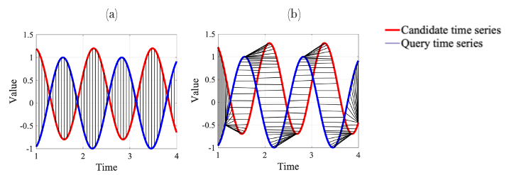
Figure 2: Alignment between two times series for calculating (a) Euclidean distance and (b) DTW distance.

DTW is often restricted to aligning points only within a moving window of a fixed size to improve accuracy and reduce computational cost. The window size may be optimized using supervised learning on the training data. When supervised learning is not possible (i.e., clustering), a window size amounting to 10% of the observation data is usually considered adequate (Ratanamahatana and Keogh,, 2004).

2.2.1 Upper and lower bounds for DTW-based distance metric

SOMTimeS uses distance bounding to prune the DTW calculations performed during the SOM unsupervised learning. This distance bounding involves finding a tight upper and lower bound. Because DTW is designed to find a mapping that minimizes the sum of the point-to-point distances between two time series, that mapping can never result in a summed distance that is greater than the sum of point-to-point Euclidean distance. Hence, finding the tight upper bound is straight forward – it is the Euclidean distance (Keogh,, 2002). To find the lower bound, we use a method – the LB_Keogh method (Keogh,, 2003), common in similarity searches (Keogh,, 2003; Ratanamahatana et al.,, 2005; Li Wei et al.,, 2005) and clustering (Begum et al.,, 2015).

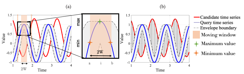
Figure 3: Two steps of calculating the L_Keogh tight lower bound for DTW in linear time: (a) determine the envelope around a query time series, and (b) sum the point to point distance shown in grey lines between the envelope and a candidate time series as LB_Keogh (Equation 2).

The LB_Keogh method comprises two steps (see Figure 3a and Figure 3b). Given a fixed DTW window size, $W$, one of the two time series (called the query time series, Q) is bounded by an envelope having an upper ($U_{i}$) and lower boundary ($L_{i}$) calculated at time step $i$, respectively, as:

$$U_{i}=\max(q_{a},...,q_{i},...,q_{b})$$ (1)

$$L_{i}=\min(q_{a},...,q_{i},...,q_{b}),$$

where $a=i-W$, and $b=i+W$ (see Figure 3a). In the second step, the LB_Keogh lower bound is calculated as the sum of Euclidean distance between the candidate time series and the envelope boundaries (see vertical lines of Figure 3b). Equation 2 shows the formula for calculating the LB_Keogh lower bound:

$$\text{LB\_Keogh}=\sqrt{\sum_{i=1}^{m}{\begin{cases}(t_{i}-U_{i})^{2},&\text{if }t_{i}>U_{i}\\ (t_{i}-L_{i})^{2},&\text{if }t_{i}<L_{i}\\ 0,&\text{otherwise}\end{cases}}}$$ (2)

where $t_{i}$, $U_{i}$, and $L_{i}$ are the values of a candidate time series, the upper and lower envelope boundary, respectively, at time step $i$.

3 The SOMTimeS Algorithm

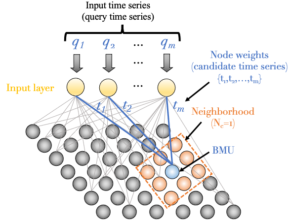
Figure 4: Schematic of the Kohonen Self-Organizing Map (after Kohnen, 2001) showing weights (candidate time series) of the best matching unit (BMU) in blue surrounded by a user-specified neighborhood ($N_{c}$).

SOMTimeS is a variant of the SOM (see Pseudocode 1), where each input observation (i.e., query time series) is compared with the weights (i.e., candidate time series) associated with each node in the 2-D SOM mesh (see Figure 4). During training, the comparison (or distance calculation) between these two time series is performed to identify the SOM node whose weights are most similar to a given input time series; this node is identified as the “best matching unit (BMU)”. Once the nodal weights (candidate time series) of the BMU have been identified, these weights (and those of the neighborhood nodes) are updated to more closely match the query time series (Line 1 of Pseudocode 1). This same process is performed for all query time series in the dataset – defined as one epoch. While iterating through some user-defined fixed number of epochs, both the neighborhood size and the magnitude of change to nodal weights are incrementally reduced. This allows the SOM to converge to a solution (stable map of clustered nodes), where the set of weights associated with these self-organized nodes now approximate the input time series (i.e., observed data). In SOMTimeS, the distance calculation is done using DTW with bounding, which helps prune the number of DTW calculations required to identify the BMU.

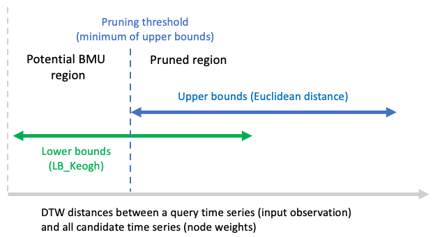
Figure 5: Identification of a qualification region in SOMTimeS.

3.1 Pruning of DTW computations

Pruning is performed in two steps. First, an upper bound (i.e., Euclidean distance) is calculated between the input observation and each weight vector associated with the SOM nodes (Line 1 of Pseudocode 1). The minimum of these upper bounds is set as the pruning threshold (see dotted line in Figure 5). Next, for each SOM node we calculate a lower bound (i.e., LB_Keogh; see Line 1). If the calculated lower bound is greater than the pruning threshold, that respective node is pruned from being the BMU. If the lower bound is less than the pruning threshold, then that SOM node lies in what we refer to as the potential BMU region (see Figure 5, and Line 1). As a result, the more expensive DTW calculations are performed only for the nodes in this potential BMU region. The node having the minimum summed distance is the BMU.

After identifying the BMUs for each input time series, the BMU weights, as well as the weights of nodes in some neighborhood of the BMUs, are updated to more closely match the respective input time series using a traditional learning algorithm based on gradient descent (Line 1 of Pseudocode 1). Both the learning rate and the neighborhood size are reduced (see lines 1 and 1) over each epoch until the nodes have self-organized (i.e., algorithm has converged). In this work, unless otherwise stated, SOMTimeS is trained for 100 epochs. To further reduce the SOM execution time, the set of input (i.e., query) time series may be partitioned in a manner similar to Wu et al., (1991), Obermayer et al., (1990) and  Lawrence et al., (1999) for parallel processing (see Line 1). We should also note that after convergence, SOMTimeS may be used to classify observations into a given number of clusters should a known number of classes exist. This is done by setting the mesh size equal to $k$ (i.e., desired number of classes), and using the weights of the BMUs for direct class assignment.

Algorithm SOMTimeS pseudocode

Input: a set $\mathcal{S}$ of query time series $\{Q_{1},Q_{2},...,Q_{n}\}$, epochs: number of epochs, $W$: warping window size

Assumption: Similarity between two observation is the DTW distance between their time series.

Output: Best Matching Units

Procedure

1 mesh_size $M$ := $5\times\sqrt{n}$    // $n$ = the number of time series in $\mathcal{S}$

2 Create and randomly initialize a mesh of Nodes[$\sqrt{M}$,$\sqrt{M}$], where the weights of each node are a randomly-generated time series (candidate time series) of length equal to the query time series.

3 neighborhood size $N_{c}$ := $\sqrt{M}/2$

4 learning rate $r$ := 0.9

5 Split $\mathcal{S}$ into subsets of equal size, $\mathcal{S}_{1},\mathcal{S}_{2},...,\mathcal{S}_{c}$, where $c$ is the number of available CPU cores in the machine.

6

7for each epoch $p$ do

8       for each split $\mathcal{S}_{i}$ ($i=1,2,...,c$) assigned to the core $i$ in parallel do

9             for each input time series $Q_{i_{j}}(j=1,2,...,n/c)$ in $\mathcal{S}_{i}$ do

10                   upper bounds:= Euclidean distances between $Q_{i_{j}}$ and weights of each node.

11                   lower bounds:= $LB\_Keogh$ between $Q_{i_{j}}$ and weights of each node using the $W$.

                   // Prune the set of all nodes to the set of qualified nodes.

12                   $Qualified$:= Set of nodes whose weights have a lower bound with $Q_{i_{j}}$ $\leq$ $\min(\text{upper bounds})$.

13                   Best matching unit:= Compute DTW distance between $Q_{i_{j}}$ and weights of nodes in $Qualified$. The best matching unit (BMU) is the node whose weights are most similar to $Q_{i_{j}}$.

14             end for

15            

16       end for

17      

18      for each time series $Q_{i}(i=1,2,...,n)$ do

             // Update the node weights of the BMU (and its neighborhood) identified for $Q_{i}$ using a gradient descent based on learning rate, to more closely match $Q_{i}$.

19            

20            for Weights ($t_{1..m}$) of BMU and its neighbor nodes do

21                   $t_{m}$ = $t_{m}+r\times(q_{m}-t_{m})$

22             end for

23            

24       end for

      // Update the neighborhood size and the learning rate in SOM.

25       $N_{c}$ := $\sqrt{M}/2\times(1-p/\textit{\#epochs})$

26       $r$ := $0.9\times(1-p/\textit{\#epochs})$

27      

28 end for

return Best matching units

Pseudocode 1 SOMTimeS algorithm pseudocode

4 Performance Evaluations

The UCR time series classification archive (Dau et al.,, 2018), with thousands of citations and downloads, is arguably the most popular archive for benchmarking time series clustering algorithms. The archive was born out of frustration, with studies on clustering and classification reporting error rates on a single time series dataset, and then implying that the results would generalize to other datasets. At the time of this writing, the archive has 128 datasets comprising a variety of synthetic, real, raw and pre-processed time series data, and has been used extensively for benchmarking the performance of clustering algorithms (e.g., Paparrizos and Gravano,, 2016, 2017; Begum et al.,, 2015; Javed et al., 2020b, ; Zhu et al.,, 2012). To evaluate SOMTimeS, we excluded sixteen of the archive datasets because they contained only a single cluster, or had time series lengths that vary. The latter prohibited a fair comparison of SOMTimeS to DTW-based K-means. The remaining 112 datasets were used to evaluate the accuracy, execution time, and scalability of SOMTimeS. We fixed the DTW window constraint at 5% of the length of the observation data following earlier recommendations by Paparrizos and Gravano, (2016, 2017).

4.1 Algorithm Assessment

Accuracy is reported using six assessment metrics (see Table 1 and Table 2) that include the Adjusted Rand Index (ARI) (Santos and Embrechts,, 2009), Adjusted Mutual Information (AMI) (Romano et al.,, 2016), the Rand Index (RI) (Hubert and Arabie,, 1985), Homogeneity (Rosenberg and Hirschberg,, 2007), Completeness (Rosenberg and Hirschberg,, 2007), and Fowlkes Mallows index (FMS) (Fowlkes and Mallows,, 1983). Scalability and execution time of DTW-based clustering algorithms are inversely affected by the length and total number of times series being clustered or classified. As a result, we report the number of DTW computations and execution time as a function of problem size, defined as $\sum_{i=1}^{n}{|Q|_{i}}$, where $|Q|$ is the length of times series $Q$, and $n$ is the total number of time series in the dataset. The presence of a few large datasets in the archive makes it more informative to visualize problem size as the logarithm to the base 10 (see Figure 1(b) in Supplementary Material). Finally, for comparison purposes, the same assessment metrics are reported for the three more popular clustering algorithms that use DTW as a distance measure — 1) K-means, 2) the SOM, and 3) TADPole. We embedded the same pruning strategy into K-means for a more equitable comparison of speed-up and clustering quality.

4.1.1 Pruning speed-up

The performance of the DTW-based SOM and K-means may be quantified in two important ways: 1) execution speed and 2) clustering quality using six different assessment indices. When pruning is not used and the number of passes (i.e., epochs) through the dataset are fixed at 10, the SOM and K-means require 13 and 14 hours, respectively, to cluster all 112 datasets in the UCR archive with comparable assessment indices (see Table 1). The SOM, however, typically requires more passes through the dataset than K-means to achieve optimal performance. When 100 epochs are used the SOM achieves a higher accuracy than K-means for 5 of the 6 measures (see Table 1); however, the execution time increases almost linearly to $\sim 148$ hours.

Table 1: Assessment of execution times and clustering quality averaged over the 112 datasets in the UCR archive for K-means and the SOM clustering methods (without pruning). Note: The six assessment indices (usually expressed as values between $0$ and $1$) have been multiplied by $100$; metric averages closer to 100 represent better performance.

Algorithm (without pruning)	Hours*	ARI		AMI		RI		H		C		FMS
		avg	std	avg	std	avg	std	avg	std	avg	std	avg	std
K-means - DTW 10-iterations	13	22	23	28	26	66	22	29	26	40	32	49	19
SOM - DTW 10-Epochs	14	21	23	27	24	70	15	28	24	31	26	47	20
SOM - DTW 100-epochs	148	24	23	30	26	71	16	31	25	35	28	50	19
*All algorithms were executed on same computational machine — dual 20-Core Intel Xeon E5-2698 v4 2.2 GHz machine with 512 GB 2,133 MHz DDR4 RDIMM.

Table 2 summarizes the execution time and six assessment indices when both the DTW-based K-means and SOM (i.e., SOMTimeS) clustering algorithms use the pruning mechanism. Additionally we present the results of TADPole (Begum et al.,, 2015), since it also uses DTW distance pruning to speedup clustering. While the speed-up times vary by dataset, DTW distance pruning improves the execution time by a factor of 2x (on average) when clustering all the 112 datasets in the UCR archive (see Figure 6). The clustering results with or without pruning are identical, and therefore, the quality (assessment indices) is the same. In comparison to TADPole, SOMTimeS is 17x faster and has a higher value in 5 out of 6 assessment indices.

Table 2: Assessment of execution times and clustering quality averaged over the 112 datasets in the UCRarchive for 1) DTW-based K-means, 2) SOMTimeS and 3) TADPole with pruning. Note: Assessment indices (usually expressed as values between $0$ and $1$) have been multiplied by $100$; metric averages closer to 100 represent better performance.

Algorithm (with pruning)	Hours*	ARI1		AMI2		RI3		H4		C5		FMS6
		avg	std	avg	std	avg	std	avg	std	avg	std	avg	std
K-means 10-iterations	6	22	23	28	26	66	22	29	26	40	32	49	19
SOMTimeS 10-Epochs	7	21	23	27	24	70	15	28	24	31	26	47	20
SOMTimeS 100-epochs	58	24	23	30	26	71	16	31	25	35	28	50	19
TADPole	1011	16	25	24	27	62	18	25	26	36	31	51	20
*All algorithms were executed on same computational machine — dual 20-Core Intel Xeon E5-2698 v4 2.2 GHz machine with 512 GB 2,133 MHz DDR4 RDIMM.

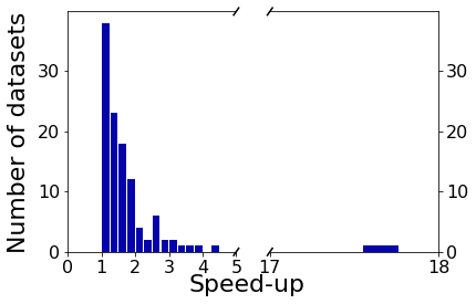
(a) SOMTimeS

(b) K-means

Figure 6: Speed-up factor achieved for different datasets in the UCR archive.

When SOMTimeS is executed in parallel, the reduction in execution time is a factor of the number of CPUs available. To cluster all 112 datasets in the UCR archive, SOMTimeS (at 100 epochs) took 3 hours using 20 CPUs, and took only 20 minutes when the number of SOM epochs was set to 10. Similar parallization can be achieved for K-means, and TADPole.

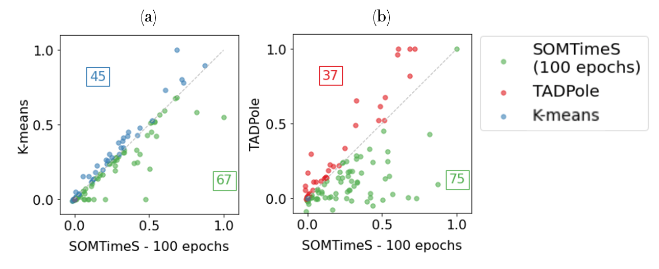
Figure 7: ARI scores for SOMTimeS (shown in green) vs. (a) TADPole (red), and (b) K-means (blue) across all 112 of the UCR datasets.

Because the ARI (Adjusted Rand Index) is recommended as one of the more robust measures for assessing accuracy across datasets (Milligan and Cooper,, 1986; Javed et al., 2020b, ), we plot the ARI scores for SOMTimeS (at 100 epochs) against K-means, and TADPole (Figures 7 (a) and (b), respectively) for each of the 112 URC datasets. The same clustering algorithm has high variation in performance metrics across datasets (Javed et al., 2020b, ). The green points (67 of the 112 datasets) lying below the 45-degree line of panel (a) represent higher accuracy for SOMTimeS, while the ARI scores above the diagonal (shown in blue) indicate that K-means outperforms SOMTimeS for 45 of the 112 datasets. The comparison of ARI scores for SOMTimeS and TADPole (Figure 7b) shows higher accuracy for SOMTimeS for 75 of the 112 datasets, and lower accuracy for the remaining 37 datasets.

4.1.2 Execution time and scalability

As mentioned previously, the speed-up achieved for SOMTimeS and K-means is a result of the pruning strategy. We study the effects of the pruning in four ways — 1) percentage of DTW computations pruned as function of time series length, 2) the total number of DTW computations pruned, 3) the scalability as a function of DTW computations performed, and 4) the change in the rate of DTW pruning over epochs.

Percentage of pruning with respect to the length of individual time series: Because DTW scales with the length of individual time series, we examined the number of DTW computations pruned as a function of time series length. Figure 8 shows the percentage of DTW computations pruned for increasing time series length on both linear and log-log scaled axes. Figure 8a shows a subset (n=36) of the UCR archived datasets. Here the subset comprises all datasets where the total number of time series is greater than 100 and the length of time series is greater than 500. Figure 8b shows the corresponding log-log plot, where the slope approximates the relationship between pruning rate and time series length. This increase in pruning rate is close to the DTW complexity of ($(m^{2}/\log\log{m})$), where $m$ is the length of time series (see Figure 8c).

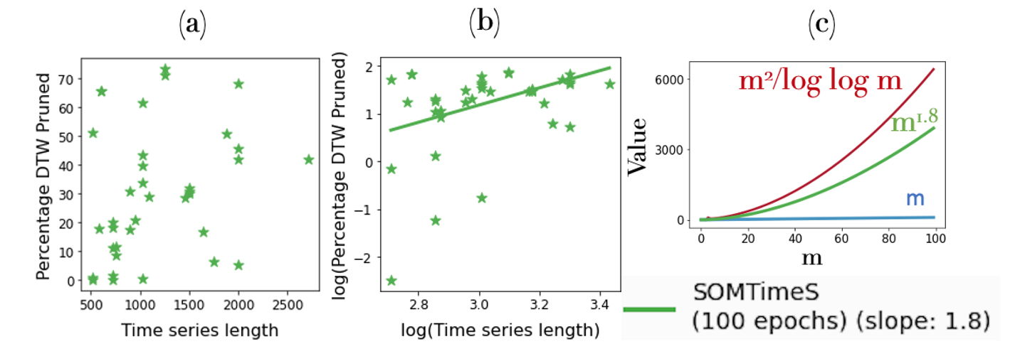
Figure 8: Percentage of DTW computations pruned with respect to the time series length shown on (a) linear scale, and (b) log-log scale axes; green stars represents one of the 36 UCR archived datasets, and (c) empirical approximation of the pruning rate as a function of time series length (m).

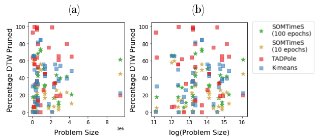
Figure S2: The pruning effect of SOMTimeS (10 epochs shown in blown stars), SOMTimeS (100 epochs in green stars), K-means (blue squares) and TADPole (red squares) measured as the percentage of DTW calls pruned during the clustering of a dataset for varying problem size in (a) linear scale axis and (b) natural log axis.

Total number of pruned DTW computations: K-means pruned more than 50% of the DTW calculations for 34 of the datasets, where as SOMTimeS (with epochs set to 10 and 100, respectively) pruned more than 50% of the DTW calculations for 8 and 21 of the 112 UCR datasets, respectively. TADPole pruned more than 50% of the DTW calculations for 40 of the datasets (see Figure S2 in Supplementary Material). Despite the apparent pruning advantage of TADPole, its quadratic complexity O($n^{2}$) with respect to DTW calculations (compared to O($n$) in SOMTimeS) results in more DTW computations, particularly for larger datasets.

Scaling of DTW computations performed as a function of number of input time series: Because TADPole performs O($n^{2}$) DTW calculations, the number of calls to DTW increases quadratically with the number $n$ of input time series. The threshold (in terms of the number of input time series, $n$) after which the number of calls to the DTW function in SOMTimeS is less than that of TADPole, depends on the number of epochs. This cutoff is empirically observed to be close to $n=100$ and $n=2500$, for 10 and 100 epochs, respectively (see Figure 9). SOMTimeS and K-means have similar theoretical and empirical complexities when the mesh size in SOMTimeS is set equal to $k$.

Overall, when clustering over all 112 of the UCR archived datasets, SOMTimeS computed the DTW measure 13 million and 100 million times (at 10 and 100 epochs, respectively). K-means computed the DTW measure 8 millions times; while TADPole by comparison computed DTW 200 million times (see Figure 9). At a dataset level, SOMTimeS had fewer calls for 12 of the datasets (when using 10 epochs) compared to K-means. At 100 epochs, SOMTimeS requires more calculations than K-means at 10 iterations to cluster all 112 datasets. In comparison to TADPole, SOMTimeS had fewer calls for 88 of the datasets (when using 10 epochs), and 26 of the datasets (for 100 epochs). However, the quality of clustering for SOMTimeS at 100 epochs increases for 4 of the six assessment indices compared to K-means, and TADPole.

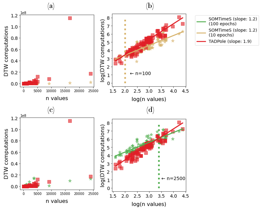
Figure 9: DTW computations performed as a function of dataset size shown on linear scaled axes (panels a and c) and log-log scale (panels b and d) for TADPole (200 million computations total) and SOMTimeS (13 million computations total at 10 epochs, and 100 million computations at 100 epochs).

Change in the SOMTimeS pruning rate as a function of epochs: When we examine the pruning effect as a function of epochs, both the number of DTW calls and the execution time decrease as the number of epochs increases. As the nodes of the SOM mesh organize, more nodes get pruned; and hence, fewer nodes exist in the unpruned region (i.e., potential BMU region of Figure 5), which decreases the need for DTW calls. Figure 10(a) shows the total number of calls to the DTW function made for each dataset, normalized over all epochs. The dashed line represents the average number of calls over all datasets and the shaded region shows the 95% confidence interval. Figure 10(b) shows the corresponding normalized execution time. Both normalized DTW calls and execution time per epoch steadily decrease with increasing number of epochs and iterative updating of SOM weights. The elbow point, where further epochs result in a diminishing reduction of DTW calculations, is at the 6th epoch. This is called the swapover point and occurs when the self-organizing map moves from gross reorganization of the SOM weights to fine-tuning of the weights.

(a)

(b)

Figure 10: Change in the SOMTimeS pruning effect as the number of epochs increases measured as the normalized (a) number of calls to the DTW function and (b) execution time. The dashed line represents the mean value for all datasets after individually normalizing each dataset run over all epochs. The shaded region corresponds to 95% confidence interval around the mean.

Finally, Figure 11 shows how SOMTimeS execution time scales with the problem size ($\sum_{i=1}^{n}{|Q|_{i}}$, where $|Q|$ is the length of times series $Q$, and $n$ is the total number of time series in the dataset). It increases at a lower rate than TADPole and is similar to K-means (with DTW distance pruning). TADPole increases at the highest rate, consistent with its O($n^{2}$) complexity of DTW calculations, followed by K-means with a complexity of O($n\times k\times$ number of iterations), where $k$ is the number of clusters. SOMTimeS has complexity of O($n\times k\times e$), where $e$ is the number of epochs. K-means (at 10 iterations) is slightly faster per unit problem size than SOMTimeS (at 10 epochs) because it 1) has pruned slightly more DTW calculations, and 2) does not require weight updates.

Figure 11: Execution time of SOMTimeS, K-means, and TADPole for the 112 archived UCR datasets on a (a) linear, and (b) log scaled axes.

5 Application to Serious Illness Conversations

We demonstrate the utility of a new artificial neural network – SOMtimeS to visualize clustered output by applying it to healthcare communication setting using actual lexical data collected in the Palliative Care Communication Research Initiative (PCCRI) cohort study (Gramling et al.,, 2015). The PCCRI is a multisite, epidemiological study that includes verbatim transcriptions of audio-recorded palliative care consultations involving 231 hospitalized people with advanced cancer, their families, and 54 palliative care clinicians.

5.1 Need for scalability in health care communication science

Understanding and improving healthcare communication requires a methodology that can measure what actually happens when patients, families, and clinicians interact in large enough samples to represent diverse cultural, dialectical, decisional and clinical contexts (Tulsky et al.,, 2017). Some features of inter-personal communication, such as tone or lexicon, will require frequent sampling over the course of conversation in order to reveal overarching patterns indicating types of interactions. Discovering patterns (i.e., clusters) of conversations with frequent sampling of features over conversation presents a need for scalable unsupervised machine learning methods. SOMTimeS is equipped to meet the need.

Our previous work suggests that conversational narrative analysis offers a clinically meaningful framework for understanding serious illness conversations (Ross et al.,, 2020; Gramling et al.,, 2021), and others have demonstrated that unsupervised machine learning can identify “types of stories” using time-series analysis of lexicon (Reagan et al.,, 2016). One core feature of conversational narrative, called temporal reference, characterizes how participants organize their conversations about things that happened in the past, are happening now, or may happen in the future (Romaine,, 1983). This motivates a study of how SOMtimeS can be useful to explore potential clusters of “temporal reference story arcs”. Natural language processing methods can reasonably estimate the shape or “arc” of temporal reference by categorizing verb tenses spoken during a conversation and describing the relative frequency of past/present/future referents over sequential deciles of total words spoken in the conversation (i.e., narrative time). In order to avoid sparse decile-level data in shorter conversations, we selected the 171 of 231 PCCRI clinical conversations as the basis for examining potential clustering.

5.2 Data pre-processing: Verb tense as a time series

We used a temporal reference tagger (Ross et al.,, 2020) to assign temporal reference (past, present, or future) to verbs and verb modifiers in the verbatim transcripts. Specifically, the Natural Language Toolkit (NLTK; www.nltk.org) was used to classify each word in the transcripts into a part of speech (POS), and for any word classified as a verb, the preceding context is used to assign that verb (and any modifiers) to a given temporal reference. Then, each conversation was stratified into deciles of “narrative time” based on the total word count for each conversation, and a temporal reference (i.e., verb tense) time series was generated for each conversation as the proportion of all future tense verbs relative to the total number of past and future tense verbs. The vertical axis in Figure 12 represents the proportion of future vs. past talk (per decile), where any value above the threshold (dashed line = 0.5) represents more future talk. Each of the 171 generated time series (see Figure 12(a)) were then smoothed using a 2nd-order, 9-step Savitzky-Golay filter (Savitzky and Golay,, 1964) (see Figure 12(b)). Savitzky-Golay filter works by fitting a polynomial over a moving window (2nd-order polynomial, over a 9-step window in this work) and replaces the data points with corresponding values of the fitted polynomial. Smoothing reduces noise that may result from simplifying assumptions used in modeling the temporal reference time series (i.e., conversational story arcs). We then used SOMTimeS to cluster the resulting conversational story arcs.

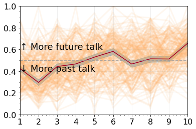
(a)

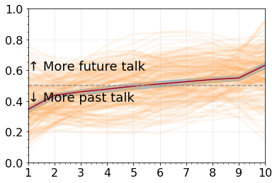
(b)

Figure 12: Temporal plot showing the (a) raw time series, and (b) smoothed time series for all conversations superimposed in brown; the red line represents the mean values, and the shaded region around the red line represents 95% confidence interval.

5.3 Clustering verb tense time series

In applying SOMTimeS to the conversational PCCRI data, we identified $k=2$ clusters with distinct temporal shapes (see Figure 13). Both of the conversational arcs share a temporal narrative with more references to the past at the beginning of the conversation, and more references to the future as the conversation progresses. The proportions of future talk and past talk are more similar at deciles 1 and 10 than at deciles 2 to 9. These conversational arcs are differentiated by the rate at which the narrative changes. Cluster 1 does not enter the “more future talk” region until decile 9, while cluster 2 does much earlier (decile 2). It was expected that the first and last deciles of the conversations would be more similar given the nature of introductionat the start and farewellat the end of a conversation.

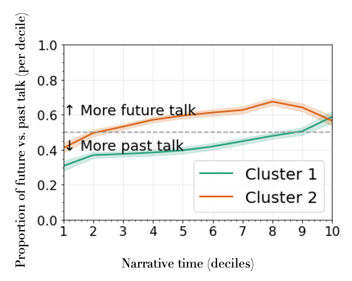
Figure 13: Mean values of the proportion of future and past (i.e., verb tense) talks over the narrative time decile for cluster 1 (green) and cluster 2 (brown) with the shaded region representing 95% confidence interval.

Now, let us illustrate how SOMTimeS identifies the number of clusters and visualizes the features that drive those clusters. When the U-matrix is superimposed on the 2-D SOM mesh (see Figure 14a), the observations appear to cluster into 2–3 groups based on visual inspection. Keeping the case study objectives in mind, and noting that the 2-D mesh is torodial, we color-coded the $k=2$ clusters on Figure 14b using spectral clustering. In Figure see 14c, we superimpose and interpolate the sum of the proportion of future vs. past talk over all deciles in the time series (i.e., conversational arcs of Figure 13) in the same 2-D space as the clustered times series.

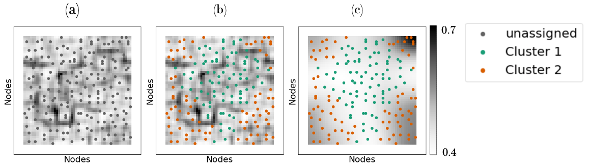
Figure 14: Temporal reference time series data from 171 serious illness conversations self-organized on a 2-D map(a) with U-matrix, (b) using spectral clustering, and (c) interpolated sum of the temporal reference time series superimposed on the clustered map.

6 Discussion

We present SOMTimeS as a clustering algorithm for time series that exploits the competitive learning of the Kohonen Self-Organizing Map, a pruning strategy and the distance bounds of DTW to improve execution time. SOMTimeS contrasts with other DTW-based clustering algorithms in both its ability to both reduce the dimensionality of, and visualize input features associated with clustering temporal data. We also implemented a similar DTW-distance pruning strategy in K-means for the first time to demonstrate performance gains achieved for what is likely the most popular clustering algorithm to date. In terms of accuracy, SOMTimeS has higher assessment indices compared to TADPole, and while the assessment indices are statistically similar with K-means, the additional functionality of the SOM comes with a higher computational cost.

The benchmark experiments in this work are intended to put SOMTimeS in context with state-of-the-art time series clustering algorithms. Keeping the study objectives in mind, execution times are used to demonstrate scalability, and highlight the feasibility of analyzing large time series datasets using SOMTimeS. K-means is perhaps the most popular clustering algorithm and has been proven time and again to outperform state-of-the-art algorithms; however, because of its simplicity, it lacks the interpretability and visualization capabilities of SOMTimeS. TADPole on the other hand, is a state-of-the-art clustering algorithm that organizes data differently from SOMTimeS (and by extension K-means), as evident from the difference in ARI scores (see Figure 7a), and choice of centroids (i.e., density peaks; see Supplementary Material Section 8.1). For these reasons, the algorithms tested are not direct competitors of one another and each has advantages in their own right.

SOMTimeS learns (i.e., self-organizes) in an iterative manner such that as the number of SOM epochs increase, the execution time per epoch decreases (see Figure 10b), making higher number of epochs (and thus, corresponding assessment indices) feasible. This reduction in time is also directly proportional to the number of calls to the DTW function at each epoch. The elbow point (at 6 for SOMTimeS with 100 epochs) indicates quick gains in pruning DTW calculations. This same gain is observed when the total number of epochs is set to 10 or 50 (see Supplementary Material Figure S3). SOMTimeS took 40 minutes to cluster the entire UCR archive using 10 epochs, and less than 300 minutes when the number of epochs was increased 10-fold. Similarly, the largest dataset in terms of problem size took 5 minutes to cluster using 10 epochs, and 35 minutes to cluster at 100 epochs. SOMTimeS demonstrates sub-linear scalability when it comes to increasing the number of epochs. The scalability, fast execution times, and the ease of saving the state (weights) of a SOM make SOMTimeS a potential candidate for an anytime algorithm. It possesses the five most desirable properties of anytime algorithms (Zilberstein and Russell,, 1995; Zhu et al.,, 2012).

Concluding Remarks:

This paper presents a computationally efficient variant of the SOM that uses DTW as a distance measure and a DTW-distance pruning strategy. To put its performance in context, two other state-of-the-art algorithms have been presented, TADPole and K-means. All three use DTW-distance pruning, and each has their own strengths and weaknesses. Firstly, they organize data differently, and secondly, the SOM is often used for data visualization, dimensionality reduction, and feature selection. For these reasons a direct comparison of the advantages and disadvantages of each algorithm is not possible, and a speed-up in one does not make the other redundant. SOMTimeS has unique data visualization abilities that require the mesh size to be increased to a value higher then $k$. The pruning strategy presented in this work makes the latter feasible. However, if only classification (or hard clusters) are required, then $k-means$ is the faster and equally accurate clustering algorithm.

7 Conclusion and Future Work

The explosion in volume of time series data has resulted in the availability of large unlabeled time datasets. In this work, we introduce Self-Organizing Maps for time series (SOMTimeS). SOMTimeS is a self-organizing map for clustering and classifying time series data that uses DTW as a distance measure of similarity between time series. To reduce run time and improve scalability, SOMTimeS prunes DTW calculations by using distance bounding during the SOM training phase. This pruning results in a computationally efficient and fast time series clustering algorithm that is linearly scalable with respect to increasing number of observations. SOMTimeS clustered 112 datasets from the UCR time series classification archive in under 5 hours with state-of-art accuracy. We also implemented a similar pruning strategy in K-means for the first time to demonstrate performance gains achieved for what is likely the most popular clustering algorithm to date. We applied SOMTimeS to 171 conversations from the PCCRI dataset. The resulting clusters showed two fundamental shapes of conversational stories.

To further improve computational efficiency and clustering accuracy, newer and state-of-the-art variations of SOMs may be used that leverage the same pruning strategy in this work. Improving computational time of DTW-based algorithms is an active area of research, and any improvement in computational speed of DTW can be incorporated in SOMTimeS for the unpruned DTW computations. Finally, SOMTimeS is a uni-variate time series clustering algorithm. To create a multivariate time series clustering algorithm, the pruning strategy will have to be revisited to accommodate the variations of DTW for multi-variate time series. SOMTimeS is a fast and linearly scalable algorithm that recasts DTW as a computationally efficient distance measure for time series data clustering.

8 Supplementary Material

This supplementary material provides additional information on the following aspects of the study:

1. Section 8.1 describes the TADPole (Begum et al.,, 2015) algorithm.

2. Figure 1(b) show datasets sorted by increasing problem size on arithmetic and log-log scale.

3. Figure 3(b) shows the percentage of DTW computations by SOMTimeS, K-means, and TADPole for each of the 112 UCR archive datasets.

4. Change in pruning efficiency of SOMTimeS (10 epochs total) as reflected by the calls to DTW function, and execution time over epochs.

8.1 TADPole

TADPole (Begum et al.,, 2015) is a density based clustering method that uses Density Peaks (Rodriguez and Laio,, 2014) as the clustering algorithm and DTW as the distance measure. The Density Peaks algorithm generates cluster centroids (called “density peaks”) that are surrounded by neighboring data points that have lower local density and are relatively farther from data points with a higher local density (Rodriguez and Laio,, 2014). The algorithm has two phases. It first finds centroids (density peaks), and then assigns data points to the closest centroid. The algorithm requires two input parameters: the number of clusters ($k$) and the local neighborhood distance $d$ (wherein the local density of a data point is calculated). In this work, when TADPole is used, $k$ is assumed to be known, and the value of $d$ is determined as the distance wherein the average number of neighbors is 1 to 2% of the total number of observations in the dataset, following a rule of thumb proposed by the original authors (Rodriguez and Laio,, 2014). TADPole uses upper bound (Euclidean distance) and lower bound (LB_Keogh) to prune unnecessary DTW calculations in the first phase to speed up the clustering. The algorithm has a complexity of O($n^{2}$) where n is the number of time series observations in the input.

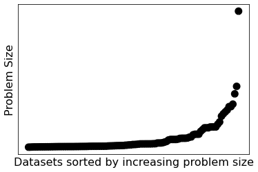
(a)

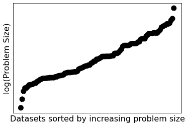
(b)

Figure S1: Distribution of all 128 datasets in the UCR archive in terms of (a) problem size and (b) natural log of problem size

.

(a) DTW calculations over epochs

(b) Execution time over epochs

Figure S3: Change in pruning efficiency of SOMTimeS (10 epochs total) as reflected by the calls to DTW function, and execution time over epochs. The dotted line represents the mean value for all datasets after individually normalizing run for each dataset over all epochs. The shaded region corresponds to 95% confidence interval around the mean.

References

- Al-Naymat et al., (2009) Al-Naymat, G., Chawla, S., and Taheri, J. (2009). Sparsedtw: A novel approach to speed up dynamic time warping. In Proceedings of the Eighth Australasian Data Mining Conference - Volume 101, AusDM ’09, pages 117–127, AUS. Australian Computer Society, Inc.
- Alvarez-Guerra et al., (2008) Alvarez-Guerra, M., González-Piñuela, C., Andrés, A., Galán, B., and Viguri, J. R. (2008). Assessment of self-organizing map artificial neural networks for the classification of sediment quality. Environment International, 34(6):782–790.
- Begum et al., (2015) Begum, N., Ulanova, L., Wang, J., and Keogh, E. (2015). Accelerating dynamic time warping clustering with a novel admissible pruning strategy. In Proceedings of the 21th ACM SIGKDD International Conference on Knowledge Discovery and Data Mining, pages 49–58.
- Bende-Michl et al., (2013) Bende-Michl, U., Verburg, K., and Cresswell, H. P. (2013). High-frequency nutrient monitoring to infer seasonal patterns in catchment source availability, mobilisation and delivery. Environmental Monitoring and Assessment, 185(11):9191–9219.
- Bentley et al., (2018) Bentley, F., Luvogt, C., Silverman, M., Wirasinghe, R., White, B., and Lottridge, D. (2018). Understanding the long-term use of smart speaker assistants. Proc. ACM Interact. Mob. Wearable Ubiquitous Technol., 2(3).
- Chu et al., (2017) Chu, E., Dunn, J., Roy, D., and Sands, G. (2017). Ai in storytelling: Machines as cocreators.
- CRS, (2020) CRS (2020). The internet of things (iot): An overview. https://fas.org/sgp/crs/misc/IF11239.pdf.
- Dau et al., (2018) Dau, H. A., Keogh, E., Kamgar, K., Yeh, C.-C. M., Zhu, Y., Gharghabi, S., Ratanamahatana, C. A., Yanping, Hu, B., Begum, N., Bagnall, A., Mueen, A., Batista, G., and Hexagon-ML (2018). The UCR time series classification archive. https://www.cs.ucr.edu/~eamonn/time_series_data_2018/.
- De Bie et al., (2016) De Bie, T., Lijffijt, J., Mesnage, C., and Santos-Rodríguez, R. (2016). Detecting trends in twitter time series. In 2016 IEEE 26th International Workshop on Machine Learning for Signal Processing (MLSP), pages 1–6.
- Ding et al., (2008) Ding, H., Trajcevski, G., Scheuermann, P., Wang, X., and Keogh, E. (2008). Querying and mining of time series data: Experimental comparison of representations and distance measures. Proc. VLDB Endow., 1(2):1542–1552.
- Dupas et al., (2015) Dupas, R., Tavenard, R., Fovet, O., Gilliet, N., Grimaldi, C., and Gascuel-Odoux, C. (2015). Identifying seasonal patterns of phosphorus storm dynamics with dynamic time warping. Water Resources Research, 51(11):8868–8882.
- Eshghi et al., (2011) Eshghi, A., Haughton, D., Legrand, P., Skaletsky, M., and Woolford, S. (2011). Identifying groups: A comparison of methodologies. Journal of data science, 9:271–291.
- Evans, (2011) Evans, D. (2011). The internet of things. how the next evolution of the internet is changing everything. Technical Report MSU-CSE-06-2, Cisco Systems.
- Ewen, (2011) Ewen, J. (2011). Hydrograph matching method for measuring model performance. Journal of Hydrology, 408(1):178 – 187.
- Flanagan et al., (2017) Flanagan, K., Fallon, E., Connolly, P., and Awad, A. (2017). Network anomaly detection in time series using distance based outlier detection with cluster density analysis. In Proceedings of the 2017 Internet Technologies and Applications, pages 116–121.
- Fowlkes and Mallows, (1983) Fowlkes, E. B. and Mallows, C. L. (1983). A method for comparing two hierarchical clusterings. Journal of the American Statistical Association, 78(383):553–569.
- Gharehbaghi and Lindén, (2018) Gharehbaghi, A. and Lindén, M. (2018). A deep machine learning method for classifying cyclic time series of biological signals using time-growing neural network. IEEE Transactions on Neural Networks and Learning Systems, 29(9):4102–4115.
- Gold and Sharir, (2018) Gold, O. and Sharir, M. (2018). Dynamic time warping and geometric edit distance: Breaking the quadratic barrier. ACM Trans. Algorithms, 14(4).
- Gramling et al., (2015) Gramling, R., Gajary-Coots, E., Stanek, S., Dougoud, N., Pyke, H., Thomas, M., Cimino, J., Sanders, M., Chang Alexander, S., Epstein, R., Fiscella, K., Gramling, D., Ladwig, S., Anderson, W., Pantilat, S., and Norton, S. (2015). Design of, and enrollment in, the palliative care communication research initiative: A direct-observation cohort study. BMC palliative care, 14:40.
- Gramling et al., (2021) Gramling, R., Javed, A., Durieux, B. N., Clarfeld, L. A., Matt, J. E., Rizzo, D. M., Wong, A., Braddish, T., Gramling, C. J., Wills, J., Arnoldy, F., Straton, J., Cheney, N., Eppstein, M. J., and Gramling, D. (2021). Conversational stories & self organizing maps: Innovations for the scalable study of uncertainty in healthcare communication. Patient Education and Counseling.
- Gupta and Chatterjee, (2018) Gupta, K. and Chatterjee, N. (2018). Financial time series clustering. In Information and Communication Technology for Intelligent Systems (ICTIS 2017), volume 2, pages 146–156.
- Hamami and Dahlan, (2020) Hamami, F. and Dahlan, I. A. (2020). Univariate time series data forecasting of air pollution using lstm neural network. In 2020 International Conference on Advancement in Data Science, E-learning and Information Systems (ICADEIS), pages 1–5.
- Hubert and Arabie, (1985) Hubert, L. and Arabie, P. (1985). Comparing partitions. Journal of Classification, 2(1):193–218.
- Iorio et al., (2018) Iorio, C., Frasso, G., D’Ambrosio, A., and Siciliano, R. (2018). A P-spline based clustering approach for portfolio selection. Expert Systems with Applications, 95:88 – 103.
- (25) Javed, A., Hamshaw, S. D., Lee, B. S., and Rizzo, D. M. (2020a). Multivariate event time series analysis using hydrological and suspended sediment data. Journal of Hydrology, page 125802.
- Javed and Lee, (2016) Javed, A. and Lee, B. S. (2016). Sense-level semantic clustering of hashtags in social media. In Proceedings of the 3rd Annual International Symposium on Information Management and Big Data.
- Javed and Lee, (2017) Javed, A. and Lee, B. S. (2017). Sense-level semantic clustering of hashtags. In Lossio-Ventura, J. A. and Alatrista-Salas, H., editors, Information Management and Big Data, pages 1–16, Cham. Springer International Publishing.
- Javed and Lee, (2018) Javed, A. and Lee, B. S. (2018). Hybrid semantic clustering of hashtags. Online Social Networks and Media, 5:23 – 36.
- (29) Javed, A., Lee, B. S., and Rizzo, D. M. (2020b). A benchmark study on time series clustering. Machine Learning with Applications, 1:100001.
- Johnpaul et al., (2020) Johnpaul, C., Prasad, M. V., Nickolas, S., and Gangadharan, G. (2020). Trendlets: A novel probabilistic representational structures for clustering the time series data. Expert Systems with Applications, 145:113119.
- Keogh, (2002) Keogh, E. (2002). Exact indexing of dynamic time warping. In Proceedings of the 28th International Conference on Very Large Data Bases, VLDB ’02, pages 406–417. VLDB Endowment.
- Keogh, (2003) Keogh, E. (2003). Efficiently finding arbitrarily scaled patterns in massive time series databases. In Lavrač, N., Gamberger, D., Todorovski, L., and Blockeel, H., editors, Knowledge Discovery in Databases: PKDD 2003, pages 253–265, Berlin, Heidelberg. Springer Berlin Heidelberg.
- Kohonen, (2013) Kohonen, T. (2013). Essentials of the self-organizing map. Neural Networks, 37:52–65. Twenty-fifth Anniversay Commemorative Issue.
- Kohonen et al., (2001) Kohonen, T., Schroeder, M. R., and Huang, T. S. (2001). Self-Organizing Maps. Springer-Verlag, Berlin, Heidelberg, 3rd edition.
- Lasfer et al., (2013) Lasfer, A., El-Baz, H., and Zualkernan, I. (2013). Neural network design parameters for forecasting financial time series. In 2013 5th International Conference on Modeling, Simulation and Applied Optimization (ICMSAO), pages 1–4.
- Lawrence et al., (1999) Lawrence, R. D., Almasi, G. S., and Rushmeier, H. E. (1999). A scalable parallel algorithm for self-organizing maps with applicationsto sparse data mining problems. Data Min. Knowl. Discov., 3(2):171–195.
- Li et al., (2020) Li, K., Sward, K., Deng, H., Morrison, J., Habre, R., Franklin, M., Chiang, Y.-Y., Ambite, J., Wilson, J. P., and P.Eckel, S. (2020). Using dynamic time warping self-organizing maps to characterize diurnal patterns in environmental exposures. Research Square.
- Li Wei et al., (2005) Li Wei, Keogh, E., Van Herle, H., and Mafra-Neto, A. (2005). Atomic wedgie: efficient query filtering for streaming time series. In Fifth IEEE International Conference on Data Mining (ICDM’05), pages 8 pp.–.
- Lou et al., (2015) Lou, Y., Ao, H., and Dong, Y. (2015). Improvement of dynamic time warping (dtw) algorithm. In 2015 14th International Symposium on Distributed Computing and Applications for Business Engineering and Science (DCABES), pages 384–387.
- Mangiameli et al., (1996) Mangiameli, P., Chen, S. K., and West, D. (1996). A comparison of som neural network and hierarchical clustering methods. European Journal of Operational Research, 93(2):402–417. Neural Networks and Operations Research/Management Science.
- Mather and Johnson, (2015) Mather, A. L. and Johnson, R. L. (2015). Event-based prediction of stream turbidity using a combined cluster analysis and classification tree approach. Journal of Hydrology, 530:751 – 761.
- Milligan and Cooper, (1986) Milligan, G. and Cooper, M. (1986). A study of the comparability of external criteria for hierarchical cluster analysis. Multivariate behavioral research, 21 4:441–58.
- Minaudo et al., (2017) Minaudo, C., Dupas, R., Gascuel-Odoux, C., Fovet, O., Mellander, P.-E., Jordan, P., Shore, M., and Moatar, F. (2017). Nonlinear empirical modeling to estimate phosphorus exports using continuous records of turbidity and discharge. Water Resources Research, 53:7590–7606.
- Obermayer et al., (1990) Obermayer, K., Ritter, H., and Schulten, K. (1990). Large-scale simulations of self-organizing neural networks on parallel computers: application to biological modelling. Parallel Computing, 14(3):381–404.
- Paparrizos and Gravano, (2016) Paparrizos, J. and Gravano, L. (2016). K-shape: Efficient and accurate clustering of time series. SIGMOD Record, 45(1):69–76.
- Paparrizos and Gravano, (2017) Paparrizos, J. and Gravano, L. (2017). Fast and accurate time-series clustering. ACM Transactions on Database Systems, 42(2):8:1–8:49.
- Parshutin and Kuleshova, (2008) Parshutin, S. and Kuleshova, G. (2008). Time warping techniques in clustering time series.
- Pirim et al., (2012) Pirim, H., Ekşioğlu, B., Perkins, A. D., and Yüceer, C. (2012). Clustering of high throughput gene expression data. Computers and Operations Research, 39:3046–3061.
- Rakthanmanon et al., (2012) Rakthanmanon, T., Campana, B., Mueen, A., Batista, G., Westover, B., Zhu, Q., Zakaria, J., and Keogh, E. (2012). Searching and mining trillions of time series subsequences under dynamic time warping. In Proceedings of the 18th ACM SIGKDD International Conference on Knowledge Discovery and Data Mining, pages 262–270.
- Ratanamahatana et al., (2005) Ratanamahatana, C., Keogh, E., Bagnall, A. J., and Lonardi, S. (2005). A novel bit level time series representation with implication of similarity search and clustering. In Ho, T. B., Cheung, D., and Liu, H., editors, Advances in Knowledge Discovery and Data Mining, pages 771–777, Berlin, Heidelberg. Springer Berlin Heidelberg.
- Ratanamahatana and Keogh, (2004) Ratanamahatana, C. A. and Keogh, E. (2004). Everything you know about Dynamic Time Warping is wrong. In Proceedings of the 3rd Workshop on Mining Temporal and Sequential Data. Citeseer.
- Reagan et al., (2016) Reagan, A. J., Mitchell, L., Kiley, D., Danforth, C. M., and Dodds, P. S. (2016). The emotional arcs of stories are dominated by six basic shapes. EPJ Data Science, 5(1).
- Rodriguez and Laio, (2014) Rodriguez, A. and Laio, A. (2014). Clustering by fast search and find of density peaks. Science, 344(6191):1492–1496.
- Romaine, (1983) Romaine, S. (1983). Locating language in time and space: William labov (ed.), quantitative analyses of linguistic structure, volume 1. academic press, new york. 271 pp. Lingua, 60(1):87–96.
- Romano et al., (2016) Romano, S., Vinh, N. X., Bailey, J., and Verspoor, K. (2016). Adjusting for chance clustering comparison measures. Journal of Machine Learning Research, 17(1):4635–4666.
- Rosenberg and Hirschberg, (2007) Rosenberg, A. and Hirschberg, J. (2007). V-measure: A conditional entropy-based external cluster evaluation measure. In Proceedings of the 2007 Joint Conference on Empirical Methods in Natural Language Processing and Computational Natural Language Learning, pages 410–420.
- Ross et al., (2020) Ross, L., Danforth, C. M., Eppstein, M. J., Clarfeld, L. A., Durieux, B. N., Gramling, C. J., Hirsch, L., Rizzo, D. M., and Gramling, R. (2020). Story arcs in serious illness: Natural language processing features of palliative care conversations. Patient Education and Counseling, 103(4):826–832.
- Sakoe and Chiba, (1978) Sakoe, H. and Chiba, S. (1978). Dynamic programming algorithm optimization for spoken word recognition. IEEE Transactions on Acoustics, Speech, and Signal Processing, 26(1):43–49.
- (59) Salvador, S. and Chan, P. (2007a). Toward accurate dynamic time warping in linear time and space. Intell. Data Anal., 11(5):561–580.
- (60) Salvador, S. and Chan, P. (2007b). Toward accurate dynamic time warping in linear time and space. Intell. Data Anal., 11(5):561–580.
- Santos and Embrechts, (2009) Santos, J. M. and Embrechts, M. (2009). On the use of the Adjusted Rand Index as a metric for evaluating supervised classification. In Proceedings of the 19th International Conference on Artificial Neural Networks: Part II, pages 175–184.
- Savitzky and Golay, (1964) Savitzky, A. and Golay, M. J. E. (1964). Smoothing and differentiation of data by simplified least squares procedures. Analytical Chemistry, 36:1627–1639.
- Silva and Henriques, (2020) Silva, M. and Henriques, R. (2020). Exploring time-series motifs through dtw-som. In 2020 International Joint Conference on Neural Networks, IJCNN, Proceedings of the International Joint Conference on Neural Networks, pages 1–8, United States. Institute of Electrical and Electronics Engineers Inc. Silva, M. I., & Henriques, R. (2020). Exploring time-series motifs through DTW-SOM. In 2020 International Joint Conference on Neural Networks, IJCNN: 2020 Conference Proceedings (pp. 1-8). [9207614] (Proceedings of the International Joint Conference on Neural Networks). Institute of Electrical and Electronics Engineers Inc.. https://doi.org/10.1109/IJCNN48605.2020.9207614; 2020 International Joint Conference on Neural Networks, IJCNN 2020 ; Conference date: 19-07-2020 Through 24-07-2020.
- Somervuo and Kohonen, (1999) Somervuo, P. and Kohonen, T. (1999). Self-organizing maps and learning vector quantization forfeature sequences. Neural Process. Lett., 10(2):151–159.
- Souto et al., (2008) Souto, M. d., Costa, I., Araujo, D., Ludermir, T., and Schliep, A. (2008). Clustering cancer gene expression data: A comparative study. BMC Bioinformatics, 9:497.
- Tulsky et al., (2017) Tulsky, J. A., Beach, M. C., Butow, P. N., Hickman, S. E., Mack, J. W., Morrison, R. S., Street, Richard L., J., Sudore, R. L., White, D. B., and Pollak, K. I. (2017). A Research Agenda for Communication Between Health Care Professionals and Patients Living With Serious Illness. JAMA Internal Medicine, 177(9):1361–1366.
- Ultsch, (1993) Ultsch, A. (1993). Self-organizing neural networks for visualisation and classification. In Opitz, O., Lausen, B., and Klar, R., editors, Information and Classification, pages 307–313, Berlin, Heidelberg. Springer Berlin Heidelberg.
- WorldEconomicForum, (2019) WorldEconomicForum (2019). How much data is generated each day? Technical report.
- Wu et al., (1991) Wu, C.-H., Hodges, R. E., and Wang, C.-J. (1991). Parallelizing the self-organizing feature map on multiprocessor systems. Parallel Computing, 17(6):821–832.
- Wu and Keogh, (2020) Wu, R. and Keogh, E. (2020). Fastdtw is approximate and generally slower than the algorithm it approximates. IEEE Transactions on Knowledge and Data Engineering, PP:1–1.
- Xi et al., (2006) Xi, X., Keogh, E., Shelton, C., Wei, L., and Ratanamahatana, C. A. (2006). Fast time series classification using numerosity reduction. In Proceedings of the 23rd International Conference on Machine Learning, ICML ’06, pages 1033–1040, New York, NY, USA. Association for Computing Machinery.
- Zhu et al., (2012) Zhu, Q., Batista, G., Rakthanmanon, T., and Keogh, E. (2012). A novel approximation to dynamic time warping allows anytime clustering of massive time series datasets. In Proceedings of the 2012 SIAM International Conference on Data Mining, pages 999–1010.
- Zilberstein and Russell, (1995) Zilberstein, S. and Russell, S. (1995). Approximate Reasoning Using Anytime Algorithms, pages 43–62. Springer US, Boston, MA.