Learning Effective and Efficient Embedding via an Adaptively-Masked Twins-based Layer

Abstract.

Embedding learning for categorical features is crucial for the deep learning-based recommendation models (DLRMs). Each feature value is mapped to an embedding vector via an embedding learning process. Conventional methods configure a fixed and uniform embedding size to all feature values from the same feature field. However, such a configuration is not only sub-optimal for embedding learning but also memory costly. Existing methods that attempt to resolve these problems, either rule-based or neural architecture search (NAS)-based, need extensive efforts on the human design or network training. They are also not flexible in embedding size selection or in warm-start-based applications. In this paper, we propose a novel and effective embedding size selection scheme. Specifically, we design an Adaptively-Masked Twins-based Layer (AMTL) behind the standard embedding layer. AMTL generates a mask vector to mask the undesired dimensions for each embedding vector. The mask vector brings flexibility in selecting the dimensions and the proposed layer can be easily added to either untrained or trained DLRMs. Extensive experimental evaluations show that the proposed scheme outperforms competitive baselines on all the benchmark tasks, and is also memory-efficient, saving 60% memory usage without compromising any performance metrics.

1. Introduction

Recently, deep learning-based recommendation models (DLRMs) have been widely adopted in many web-scale applications such as recommender systems (Cheng et al., 2016; Guo et al., 2017; Wang et al., 2017; Lian et al., 2018; Li et al., 2019; Juan et al., 2016). One of the main parts of DLRMs is the embedding layer, which exploits the categorical features. A standard embedding layer maps the categorical feature to an embedding space (Guo et al., 2017; Cheng et al., 2016; Wang et al., 2017). Specifically, given a feature field $F$ and let its vocabulary size be $|F|$, each feature value $f_{i}\in F$ is mapped to an embedding vector by an embedding matrix $W\in\mathbb{R}^{|F|\times D}$, where $D$ is a predefined embedding dimension.

However, the above standard method can lead to two problems. First, in real applications, different feature values in the same feature field can have significantly different frequencies. For high-frequency feature values, it is necessary to use a sufficiently large embedding dimension to express rich information. Meanwhile, assigning too large embedding dimensions to low-frequency feature values is prone to over-fitting issues. Therefore, a fixed and uniform embedding dimension for all the feature values in a feature field can undermine effective embedding learning for different feature values. Second, storing the embedding matrix with a fixed and uniform dimension may result in a huge memory cost (Zhang et al., 2020; Shi et al., 2020; Zhao et al., 2020a). A flexible dimension assignment is needed to reduce the memory cost.

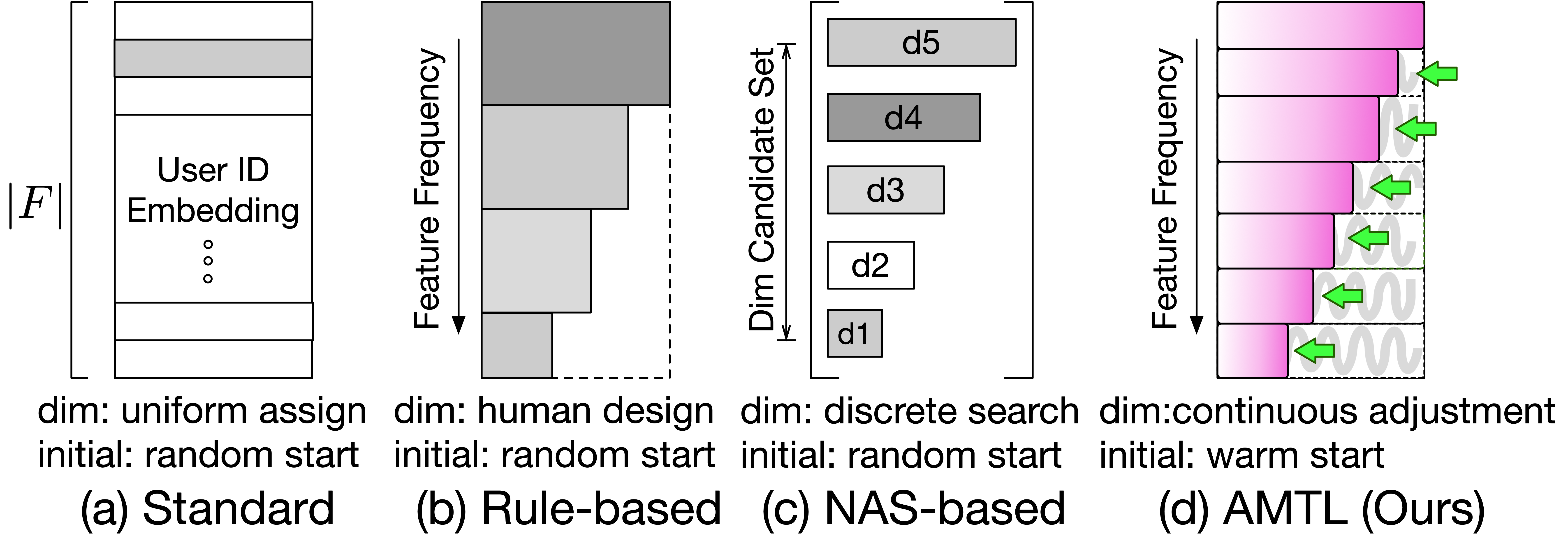
Figure 1. Comparison among existing methods and ours.

There are some existing works trying to learn unfixed and nonuniform embedding dimensions for different feature values. They can be primarily divided into two categories. (1) Rule-based methods adopt human-defined rules, typically according to the feature frequencies, to give different embedding dimensions to different feature values (Ginart et al., 2019) (see Fig. 1 (b) for an example). The problem with this category of methods is that they heavily rely on human knowledge and human labor. The resulting rough dimension selection for groups of feature values can often lead to poor performance (see Section 3.2). (2) Neural architecture search (NAS)-based methods use NAS techniques to search from several candidate embedding dimensions to find a suitable one for each feature value (Zhao et al., 2020a; Zhao et al., 2020b; Joglekar et al., 2020; Liu et al., 2020) (see Fig 1 (c) for an example). These methods require careful design of the search space and training-searching strategies. The search space is usually limited to a restricted set of discrete dimensions. Besides, both categories of methods mentioned above require training (i.e., embedding learning) from scratch. However, in real applications, there may exist some embedding matrices already trained with a huge amount of data. Such embedding matrices can be utilized for warm starting (see Section 3.4). Unfortunately, existing methods are not friendly to accommodate such a warm start mechanism.

In this paper, we propose a novel and effective method to select proper embedding dimensions for different feature values. The basic idea is to add an Adaptively-Masked Twins-based Layer (AMTL) on top of the embedding layer. Such a layer can adaptively learn a mask vector to mask the undesired dimension of the embedding vector for each feature value. The masked embedding vectors can be taken as the vectors with adaptive dimensions and are fed into the subsequent processes in DLRMs. This method exhibits some nice properties. First, it is effective for embedding learning because the embedding dimension of different feature values can be learned and adjusted in continuous integer space with sufficient flexibility without human interaction or specific NAS design (see Section 3.2). Second, it is efficient since a memory-efficient model can be built by adjusting the embedding dimension (see Section 3.3). Third, the parameters of the embedding matrix can be efficiently trained with the warm start mechanism (see Section 3.4).

We summarize our contributions as follows: (1) We propose a novel embedding dimension selection method that completely removes the necessity of human rules or NAS architectures to facilitate adaptive dimension learning. (2) The proposed method (AMTL) can be easily applied in trained DLRMs to facilitate a warm start. The twins-based architecture successfully tackles the sample unbalance problem. (3) Extensive experimental results demonstrate that the proposed method outperforms strong baseline methods. The nice properties of AMTL helped us reduce memory cost by up-to 60% without compromising any performance metrics, and can further improve the performance by the warm start mechanism.

2. Method

2.1. Basic Idea

We first recall a standard embedding layer which can be expressed as $e_{i}=W^{T}v_{i}$ where $v_{i}$ is a one-hot vector for the feature value $f_{i}$, $W\in\mathbb{R}^{|F|\times D}$ refers to the embedding table and $e_{i}\in\mathbb{R}^{D}$ is the embedding vector of $f_{i}$. Then we define a mask vector $m_{i}\in\{0,1\}^{D}$ for $f_{i}$. This mask vector should satisfy

(3) $$m_{i,j}=\left\{\begin{array}[]{lc}1&j\leq k_{i}\\ 0&j>k_{i}\end{array}\right.$$

where $k_{i}\in[0,D-1]$ is a learnable integer parameter which is influenced by the frequency of $f_{i}$. Then, to allow different $f_{i}$ can adjust its embedding dimension, the basic idea is that we can use the mask vector $m_{i}$ to mask the embedding vector $e_{i}$, i.e., $\hat{e}_{i}=m_{i}\odot e_{i}$ where $\odot$ represents the element-wise multiply. Since the value whose index is larger than $k_{i}$ in $\hat{e}_{i}$ is zero, the masked embedding vector $\hat{e}_{i}$ can be taken as an embedding vector where the embedding dimension is adaptively adjusted by the mask vector, and the first $k_{i}+1$ dimensions (i.e., from 0-th to $k_{i}$-th dimension) of $e_{i}$ is selected.

Memory Saving. When storing $\hat{e}_{i}$, we can simply drop the zero values in $\hat{e}_{i}$ to save memory and when fetching the stored vector, we can simply re-pad zero values to recover $\hat{e}_{i}$.

Embedding Usage. When embedding vectors are assigned with different dimensions, all of the existing methods (Ginart et al., 2019; Zhao et al., 2020a; Zhao et al., 2020b; Joglekar et al., 2020; Liu et al., 2020) have to design an additional layer to unify these vectors to a same length to fit the following uniform MLP layers in DLRMs. Unlike these methods, our method does not need any additional layers since the masked embedding vectors $\hat{e}_{i}$ have the same length by zeros paddings, and can be directly fed into the following layers.

Why select first $k_{i}+1$ dimensions? In this paper, We take the strategy about selecting first $k_{i}+1$ dimensions (i.e., from 0-th to $k_{i}$-th dimension) of $e_{i}$ as an example and others (e.g., selecting last $k_{i}+1$ dimensions) are also allowed. One should keep in mind is that the select strategy should follow some rules. In other words, randomly selecting $k_{i}+1$ dimensions of $e_{i}$ is not a good strategy because we can hardly directly drop and recover these zeros values in $\hat{e}_{i}$ to save memory due to the random distribution of zeros values in $\hat{e}_{i}$, and it also prevents the model to characterize each feature value since the same feature value may be mapped to different embedding vectors due to the random selection.

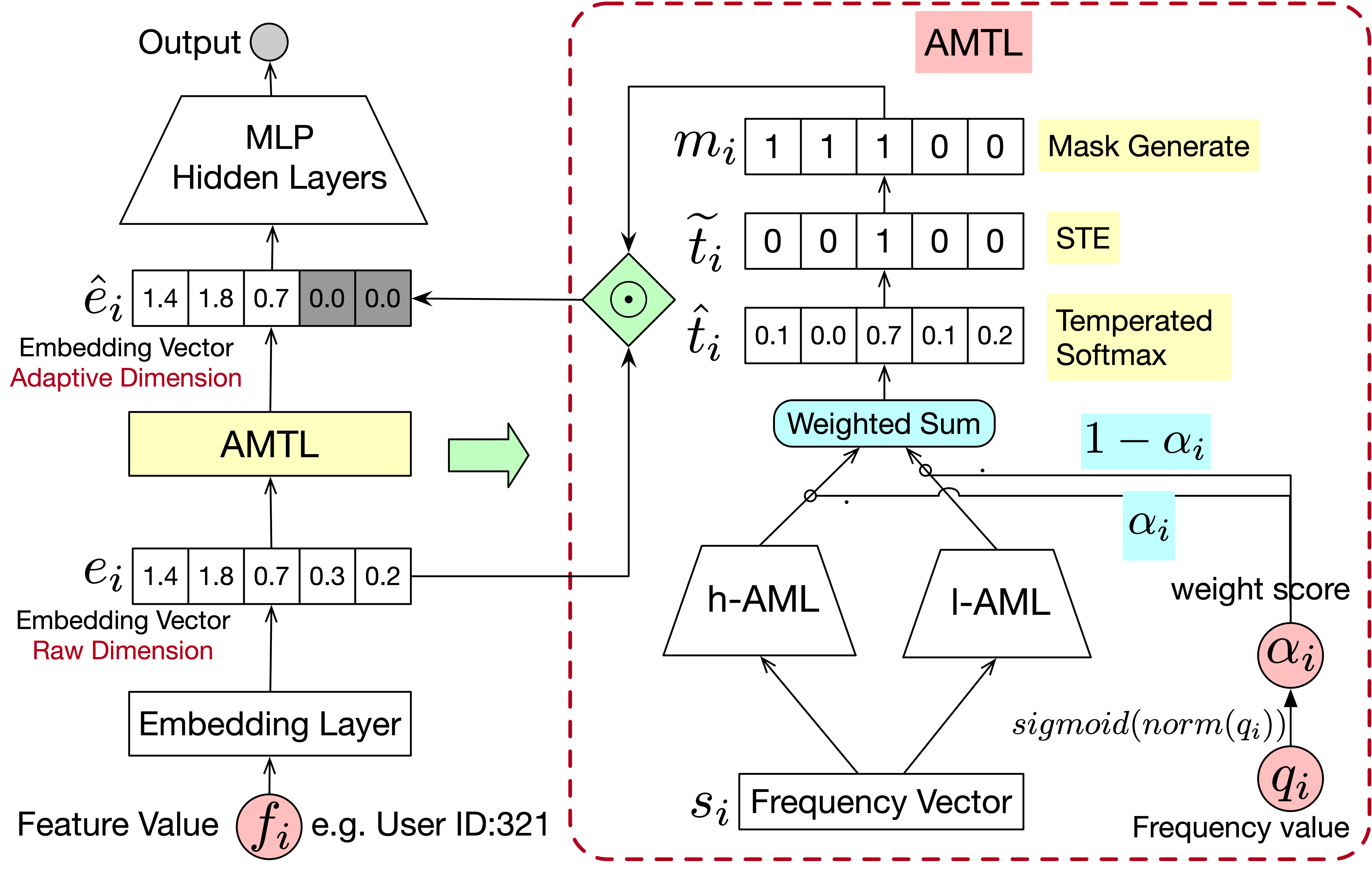
Figure 2. The framework of AMTL.

2.2. Adaptively-Masked Twins-based Layer

Adaptively-Masked Twins-based Layer (AMTL) is designed to generate a mask vector $m_{i}$ in Eq 3 for each feature value $f_{i}$. The framework of AMTL is shown in Fig 2.

2.2.1. Input and Output

Input: Since $m_{i}$ is required to be adjusted by the feature frequency, to allow AMTL to have such frequency knowledge, we take the frequency attribute (e.g., the appear times in history, the frequency rank in this feature field and so no) of $f_{i}$ as the input of AMTL. The input sample is denoted as $s_{i}\in R^{z}$ and $z$ is the input dimension. Output: The output of AMTL is a one-hot vector (called selection vector) to represent $k_{i}$ in Eq 3.

2.2.2. Architecture

We propose a twins-based (i.e., two branches) architecture and each branch is an Adaptively-Masked Layer (AML). Note parameters of the two branches are not sharing. Both of AML is a multilayer perceptron: $h_{l}=\sigma(W_{l}^{T}\;h_{l-1}+b_{l})$ where $h_{0}$ is the frequency vector, $W_{l}$ and $b_{l}$ are the parameters of the $l$-th layer, $\sigma$ is an activation function and $h_{L}\in\mathbb{R}^{D}$ is the output of the last layer.

The motivation of such twins design is that if we only take a single branch (i.e., AML), the parameters update of AML will be dominated by the high-frequency feature values due to the unbalanced problem. Specifically, since high-frequency feature values appear more times in samples, the major part of the input sample of AML represents high-frequency vectors. Then, the parameters of AML may be heavily influenced by the high-frequency vectors and AML may blindly select large embedding dimensions. Hence we design twins-based architecture to address this problem where the two branches (i.e., h-AML and l-AML) are used for high- and low- frequency samples respectively. In this way, the parameters of the l-AML will not be dominated by high-frequency samples and can give an unbiased decision.

Weighted Sum. However, one challenge is that we can hardly give a threshold to differentiate the high- and low- frequency samples to feed different samples to different branches. Hence, we propose a soft decision strategy. Specifically, we define the frequency value of $f_{i}$ as $q_{i}$ which refers to the present times of $f_{i}$ in history, and feed the input sample $s_{i}$ into h-AML and l-AML respectively. A weighted sum is applied on the $L$-th outputs (i.e., $h_{L}^{(\textit{h-AML})}\in\mathbb{R}^{D}$ and $h_{L}^{(\textit{l-AML})}\in\mathbb{R}^{D}$ ) of h-AML and l-AML, i.e.,

(4) $$h_{L}^{(\textit{AMTL})} =\alpha_{i}*h_{L}^{(\textit{h-AML})}+(1-\alpha_{i})*h_{L}^{(\textit{l-AML})}$$

(5) $$\alpha_{i} =sigmoid(norm(q_{i}))$$

where $\alpha_{i}\in[0,1]$ is the weight score which is influenced by $q_{i}$. $norm$ operation normalizes $q_{i}$ to a standard normal distribution which allows $\alpha_{i}$ is distributed smoothly around $1/2$. Otherwise, all $\alpha_{i}$ may be close to one without the $norm$ operation. In this way, for the samples with high-frequency, the corresponding $h_{L}^{(\textit{AMTL})}$ is dominated by $h_{L}^{(\textit{h-AML})}$ due to a large $\alpha_{i}$. Then the parameters of h-AML are mainly updated during back-propagation and vice versa. Hence, AMTL can adjust the gradients of h-AML and l-AML to address the unbalanced problem. Note here we only give an example to calculate the weight value $\alpha_{i}$, other ways are also allowed as long as the produced $\alpha_{i}$ has similar properties.

Then we apply softmax function on $h_{L}^{(\textit{AMTL})}$, i.e.,

(6) $$o_{i,p}=exp(h_{L,p}^{(\textit{AMTL})})/{\textstyle\sum_{j}}exp(h_{L,j}^{(\textit{AMTL})})$$

where $o_{i}\in\mathbb{R}^{D}$ refers the probability to select different embedding dimension of $f_{i}$, and $o_{i,p}$ is the $p$-th element of $o_{i}$. The selection vector can be obtained by

(7) $$t_{i}=one\_hot(argmax_{p}(o_{i,p}))$$

Then the corresponding mask vector can be generated by

(8) $$m_{i} =M^{T}t_{i}$$

where $M\in\mathbb{R}^{D\times D}$ is a pre-defined mask matrix and $M_{i,j}=1$ when $j\leq i$ otherwise $M_{i,j}=0$. Then the masked embedding $\hat{e}_{i}$ can be obtained by $m_{i}$. Note in practice, we usually apply different AMTLs on different important feature fields (e.g., User ID and Item ID) and the parameters of these layers are not sharing for the purpose of field awareness.

2.2.3. Relaxation

However, the problem is that the learning process of AMTL is non-differentiable due to the discrete process in Eq 7. It means the parameters of AMTL cannot be directly optimized by a stochastic gradient descent (SGD). To address this problem, we relax $t_{i}$ to a continuous space by temperated softmax (Hinton et al., 2015; Jang et al., 2016; Maddison et al., 2016). Concretely, the $p$-th element of $t_{i}$ can be approximated as

(9) $$t_{i,p}\approx\hat{t}_{i,p}=exp(h_{L,p}^{(AMTL)}/T)/{{\textstyle\sum_{j}}(exp(h_{L,j}^{(AMTL)}/T)}$$

where $T$ is the temperature hyper-parameter. When $T\rightarrow 0$, this approximation becomes exact. Since $\hat{t}_{i}$ is a continuous vector with differentiable process, SGD can be naturally applied. Hence, instead of learning the discrete vector $t_{i}$, we learn $\hat{t_{i}}$ to approximate $t_{i}$.

However, there exists an information gap between training and inference phases when using temperature softmax. Specifically, we use the vector $\hat{t}_{i}$ for training. While in inference, we only use the discrete vector $t_{i}$. To close this gap, inspired by the idea Straight-Through Estimator (STE) (Bengio et al., 2013), we rewrite $t_{i}$ as

(10) $$\widetilde{t}_{i}=\hat{t}_{i}+stop\_gradient(t_{i}-\hat{t}_{i})$$

where stop_gradient is used to prevent the gradient from back-propagation through it. Since the forward pass is not affected by stop_gradient, $\widetilde{t}_{i}=t_{i}$ during this phase. For the back-propagation, it avoids the non-differentiable process by stop_gradient.

3. Experiments

3.1. Experiment Setup

Data Sets. (1) MovieLens is a user review data about movies and is collected from MovieLens website. There are a total of 1,000,209 records. (2) IJCAI-AAC is collected from a sponsored search in E-commerce. There are a total of 478,138 records. (3) Taobao Dataset is an industrial dataset which is constructed from Taobao. There are a total of 50 billion around records.

Baselines. We consider different kinds of state-of-the-art embedding methods as baselines (1) Standard: traditional Fixed-based Embedding (FBE). (2) Rule-Based: MDE (Ginart et al., 2019) divides different feature values into several blocks by their frequency, and assigns different embedding dimensions for different blocks by rules. (3) NAS-Based: AutoEmb (Zhao et al., 2020b) adopts NAS to select embedding dimensions among some candidate embedding dimensions for different feature values.

Table 1. The results about CTR tasks.

AUC(%) FBE MDE AutoEmb AMTL IJCAI-AAC 62.37 62.40 62.85 63.45 MovieLens 80.84 80.51 81.28 81.50 Taobao 73.64 73.54 73.67 74.02

Setting. The maximal embedding dimension and the DLRM bone-skeleton of all methods are set the same. The dimension selection strategy is applied to the feature fields which are related to the user and item property (e.g., User ID and Item ID). For AutoEmb, the candidate dimension list is set smoothly by following the original paper (Zhao et al., 2020b). The temperature $T$ in Eq 9 is set by grid search.

Table 2. Memory cost comparison.

Methods	FBE	MDE	AutoEmb	AMTL
Avg(Dim)	300	170	206	110
Ratio	100%	56.7%	68%	36.7%

3.2. Click-Through Rate Prediction Tasks

Here, we compare our method AMTL with baselines on click-through rate (CTR) prediction tasks and take the AUC (Fawcett, 2006) score as the metric. Note a slightly higher AUC at 0.1%-level is regarded as significant for the CTR task (Zhou et al., 2018; Song et al., 2019). As shown in Table 1, we can conclude that: (1) Compared with FBE, AMTL can archive better performance in all datasets. It shows that adopting an unfixed embedding dimension can improve the model performance. (2) Compared with the rule-based method (i.e., MDE), AMTL outperforms MDE. Besides, MDE only obtains similar performance with FBE. It indicates a rough human rule on dimension selection cannot always guarantee an improvement. (3) For the NAS-based method (AutoEmb), AMTL also archives better performance. It demonstrates that AMTL adopts a more suitable scheme i.e., selecting a dimension from a continuous integer space.

3.3. Memory Cost Comparison

Here, we compare the memory cost of different methods. Since the memory size of the embedding matrix is in direct proportion to the dimension (Zhang et al., 2020; Shi et al., 2020), for simplicity, the averaged dimension (i.e., Avg(Dim)) are reported. We take the feature field ”User ID” in Taobao as an example (others can have similar conclusions), and its’ maximal dimension is set as 300. Table 2 shows the results. We also show the Avg(Dim) ratio compared with FBE. We can find that (1) Compared with FBE, all the dimension selection methods can save memory size by reducing the embedding to a suitable dimension. (2) Since AMTL allows a more flexible dimension selection in a continuous integer space, it reduces memory cost more significantly by around 60 %.

Table 3. The results of warm start.

AUC(%)	FBE	MDE	AutoEmb	AMTL
Warm Start	77.05	75.43	75.62	77.22
Random Start	73.64	73.54	73.67	74.02

Table 4. The results of ablation study.

	FBE	AMTL	AML	AMTL-nSTE
AUC(%)	62.37	63.45	62.97	63.01

3.4. Evaluation for the Warm Start

Here, we conduct experiments to evaluate the warn start on the dataset Taobao which is close to the industrial and real system. There are two kinds of parameters in DLRM, i.e., the parameters of embedding matrix and hidden layers. In the warm start setting, for existing dimension selection methods, we initialize the parameters of hidden layers by loading the parameters from the online model in Taobao, and the parameters of embedding matrix are randomly initialized due to the inability on the warm start of embedding matrix. While, since AMTL and FBE can warm start the parameters both of the embedding matrix and the hidden layers, we load both of them from the online model for these two methods. The results are shown in Table 3. The results of random start are also provided. We can find that compared with MDE and AutoEmb, AMTL can perform better in the warm start setting. Specifically, compared with the best baseline AutoEmb, the gain of AMTL is 1.6% in the warm start manner, which is 5$\times$ times larger than the gain in the random start manner. Furthermore, due to the inability for the warm start of the embedding matrix, MDE and AutoEmb even perform worse than the standard full embedding. It demonstrates that the dimension selection scheme designed in AMTL is a more wise and flexible way in real application systems.

3.5. Evaluation for Frequency

Here we analyze whether AMTL can give suitable dimensions for different feature values. Specifically, we divide the feature value into 7 groups (i.e., $G_{i},i\in\{0,1,2,...,6\}$) by frequency and the average frequency of different groups is increased from $G_{0}$ to $G_{6}$. Note there are too many feature fields in different datasets, we take the feature field ”User ID” in Taobao as an example, and others have similar results. The averaged embedding dimension in different groups is reported in Fig 3 (a). It shows that when the frequency increases (i.e., from $G_{0}$ to $G_{6}$), the selected average dimension is increased. It indicates AMTL can assign suitable embedding dimensions to different frequency feature values adaptively.

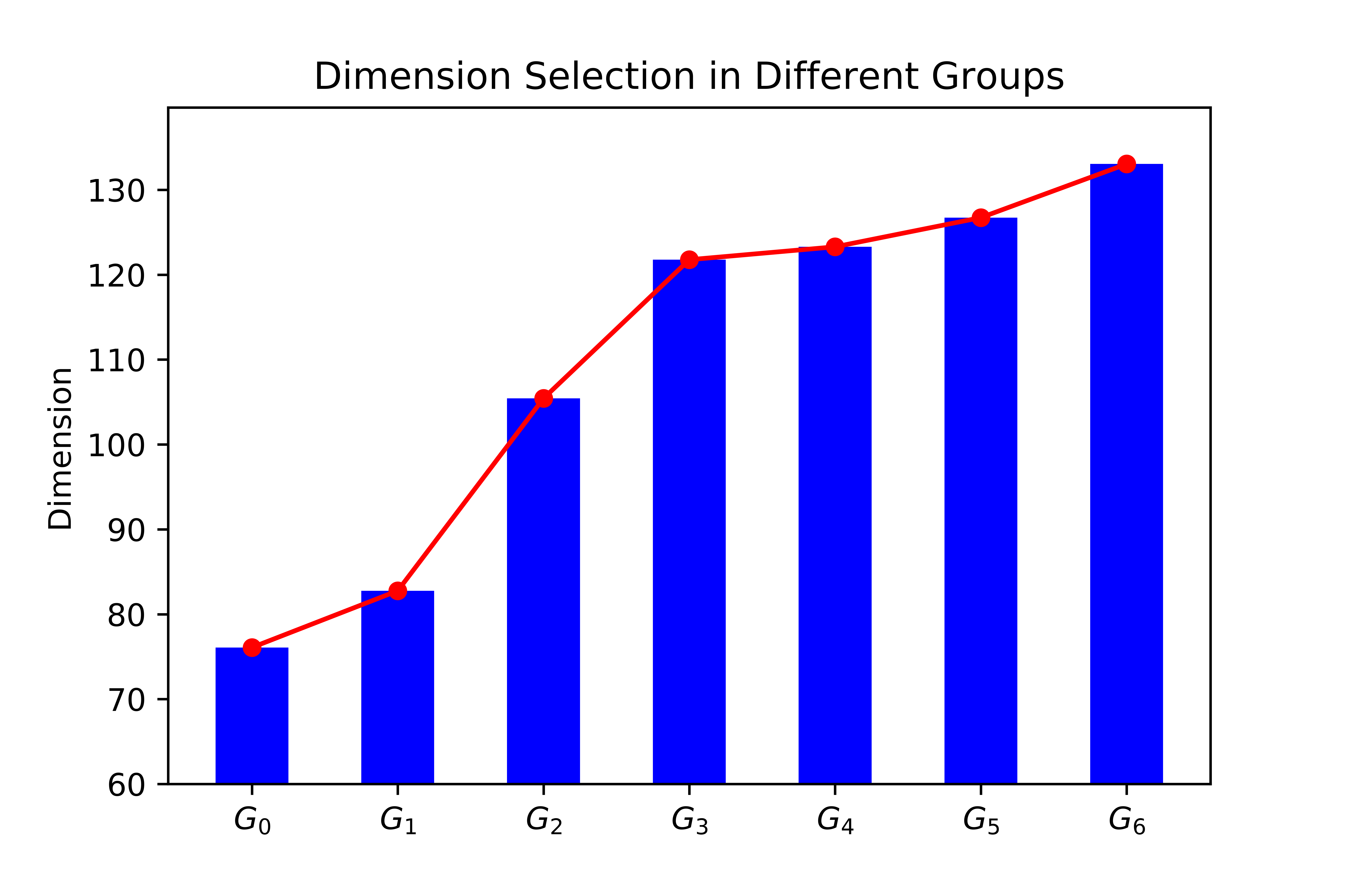
(a) AMTL

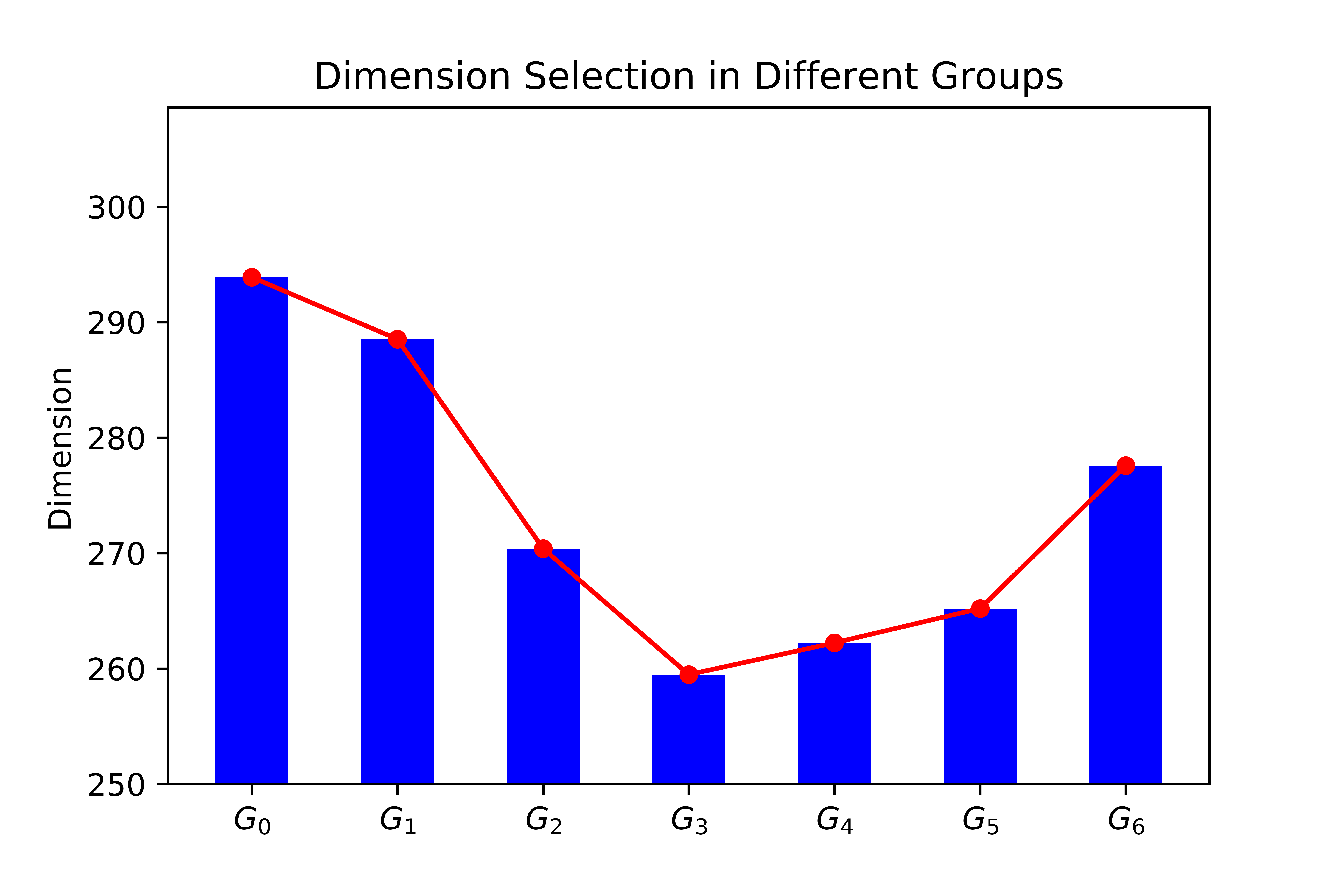
(b) AML

Figure 3. Dimension section of AMTL and AML.

3.6. Ablation Study

Here, we conduct an ablation study on the twins-based architecture and STE. Due to the limited space, the results on IJCAI-AAC are reported and similar conclusions can be found from other datasets.

Evolution on twins-based architecture. We compared the AUC score between AMTL and AML (only a single branch) on CTR task. From Table 4, although both AML and AMTL perform better than FBE, AMTL archives a higher performance. It indicates twins-based architecture plays an important role in feature learning. Besides, similar to Section 3.5, we also visualize the dimension selection of AML in Fig 3 (b). We can find that AML only successfully gives suitable dimensions in high-frequency groups (i.e., $G_{3}$ to $G_{6}$). In low-frequency groups, due to the unbalanced problem, it blindly gives high dimensions for low-frequency values. And the lower the frequency, the worse it is.

Evolution on STE. Here, we analyze the effectiveness of STE, and implement a variant of AMTL without STE, denoted as AMTL-nSTE. From Table 4, compared with AMTL-nSTE, AMTL can archive better performance. It demonstrates the usefulness to bridge the information gap between training and inference phases by STE.

3.7. Time Cost Analysis

In this section, we conduct experiments to report the time cost per epoch of different methods on IJCAI-AAC (similar conclusions can be found in other datasets). As shown in Table 5, we find that compared with FBE, the dimension selection methods need more time to train the model per epoch due to the dimension selection processes. During inference, we can directly look up the learned embedding table which has adaptive dimensions without the process of dimension selection to save time.

Table 5. The time cost of different methods

	FBE	MDE	AutoEmb	AMTL
per epoch (s)	13.3	13.8	15.7	14.5

4. Conclusion

Traditional embedding learning methods usually adopt a fixed dimension for all features which may cause problems in space complexity and performance. To address this problem, we propose a novel dimension selection method called AMTL which produces a mask vector to mask the undesired dimensions for different feature values. Experimental results show that the proposed method can archive the best performance on all tasks especially in the case of embedding warm start, give a suitable dimension for different features and save memories at the same time.

References

- (1)
- Bengio et al. (2013) Yoshua Bengio, Nicholas Léonard, and Aaron Courville. 2013. Estimating or propagating gradients through stochastic neurons for conditional computation. arXiv preprint arXiv:1308.3432 (2013).
- Cheng et al. (2016) Heng-Tze Cheng, Levent Koc, Jeremiah Harmsen, Tal Shaked, Tushar Chandra, Hrishi Aradhye, Glen Anderson, Greg Corrado, Wei Chai, Mustafa Ispir, et al. 2016. Wide & deep learning for recommender systems. In Proceedings of the 1st workshop on deep learning for recommender systems. 7–10.
- Fawcett (2006) Tom Fawcett. 2006. An introduction to ROC analysis. Pattern recognition letters 27, 8 (2006), 861–874.
- Ginart et al. (2019) Antonio Ginart, Maxim Naumov, Dheevatsa Mudigere, Jiyan Yang, and James Zou. 2019. Mixed dimension embeddings with application to memory-efficient recommendation systems. arXiv preprint arXiv:1909.11810 (2019).
- Guo et al. (2017) Huifeng Guo, Ruiming Tang, Yunming Ye, Zhenguo Li, and Xiuqiang He. 2017. DeepFM: a factorization-machine based neural network for CTR prediction. arXiv preprint arXiv:1703.04247 (2017).
- Hinton et al. (2015) Geoffrey Hinton, Oriol Vinyals, and Jeff Dean. 2015. Distilling the knowledge in a neural network. arXiv preprint arXiv:1503.02531 (2015).
- Jang et al. (2016) Eric Jang, Shixiang Gu, and Ben Poole. 2016. Categorical reparameterization with gumbel-softmax. arXiv preprint arXiv:1611.01144 (2016).
- Joglekar et al. (2020) Manas R Joglekar, Cong Li, Mei Chen, Taibai Xu, Xiaoming Wang, Jay K Adams, Pranav Khaitan, Jiahui Liu, and Quoc V Le. 2020. Neural input search for large scale recommendation models. In Proceedings of the 26th ACM SIGKDD International Conference on Knowledge Discovery & Data Mining. 2387–2397.
- Juan et al. (2016) Yuchin Juan, Yong Zhuang, Wei-Sheng Chin, and Chih-Jen Lin. 2016. Field-aware factorization machines for CTR prediction. In Proceedings of the 10th ACM conference on recommender systems. 43–50.
- Li et al. (2019) Feng Li, Zhenrui Chen, Pengjie Wang, Yi Ren, Di Zhang, and Xiaoyu Zhu. 2019. Graph Intention Network for Click-through Rate Prediction in Sponsored Search. In Proceedings of the 42nd International ACM SIGIR Conference on Research and Development in Information Retrieval. 961–964.
- Lian et al. (2018) Jianxun Lian, Xiaohuan Zhou, Fuzheng Zhang, Zhongxia Chen, Xing Xie, and Guangzhong Sun. 2018. xdeepfm: Combining explicit and implicit feature interactions for recommender systems. In Proceedings of the 24th ACM SIGKDD International Conference on Knowledge Discovery & Data Mining. 1754–1763.
- Liu et al. (2020) Haochen Liu, Xiangyu Zhao, Chong Wang, Xiaobing Liu, and Jiliang Tang. 2020. Automated Embedding Size Search in Deep Recommender Systems. In Proceedings of the 43rd International ACM SIGIR Conference on Research and Development in Information Retrieval. 2307–2316.
- Maddison et al. (2016) Chris J Maddison, Andriy Mnih, and Yee Whye Teh. 2016. The concrete distribution: A continuous relaxation of discrete random variables. arXiv preprint arXiv:1611.00712 (2016).
- Shi et al. (2020) Hao-Jun Michael Shi, Dheevatsa Mudigere, Maxim Naumov, and Jiyan Yang. 2020. Compositional embeddings using complementary partitions for memory-efficient recommendation systems. In Proceedings of the 26th ACM SIGKDD International Conference on Knowledge Discovery & Data Mining. 165–175.
- Song et al. (2019) Weiping Song, Chence Shi, Zhiping Xiao, Zhijian Duan, Yewen Xu, Ming Zhang, and Jian Tang. 2019. Autoint: Automatic feature interaction learning via self-attentive neural networks. In Proceedings of the 28th ACM International Conference on Information and Knowledge Management. 1161–1170.
- Wang et al. (2017) Ruoxi Wang, Bin Fu, Gang Fu, and Mingliang Wang. 2017. Deep & cross network for ad click predictions. In Proceedings of the ADKDD’17. 1–7.
- Zhang et al. (2020) Caojin Zhang, Yicun Liu, Yuanpu Xie, Sofia Ira Ktena, Alykhan Tejani, Akshay Gupta, Pranay Kumar Myana, Deepak Dilipkumar, Suvadip Paul, Ikuhiro Ihara, et al. 2020. Model Size Reduction Using Frequency Based Double Hashing for Recommender Systems. In Fourteenth ACM Conference on Recommender Systems. 521–526.
- Zhao et al. (2020a) Xiangyu Zhao, Haochen Liu, Hui Liu, Jiliang Tang, Weiwei Guo, Jun Shi, Sida Wang, Huiji Gao, and Bo Long. 2020a. Memory-efficient Embedding for Recommendations. arXiv preprint arXiv:2006.14827 (2020).
- Zhao et al. (2020b) Xiangyu Zhao, Chong Wang, Ming Chen, Xudong Zheng, Xiaobing Liu, and Jiliang Tang. 2020b. AutoEmb: Automated Embedding Dimensionality Search in Streaming Recommendations. arXiv preprint arXiv:2002.11252 (2020).
- Zhou et al. (2018) Guorui Zhou, Xiaoqiang Zhu, Chenru Song, Ying Fan, Han Zhu, Xiao Ma, Yanghui Yan, Junqi Jin, Han Li, and Kun Gai. 2018. Deep interest network for click-through rate prediction. In Proceedings of the 24th ACM SIGKDD International Conference on Knowledge Discovery and Data Mining. ACM, 1059–1068.