Inverse Sampling of Degenerate Datasets from a Linear Regression Line
Abstract
When linear regression generates a relationship between a (dependent) scalar response and one or multiple independent variables, various datasets providing distinct graphical trends can develop resembling relationships based on the same statistical properties. Advanced statistical approaches, such as neural networks and machine learning methods, are of great necessity to process, characterize, and analyze these degenerate datasets. On the other hand, the accurate creation of purposedly degenerate datasets is essential to test new models in the research and education of applied statistics. In this light, the present study characterizes the famous Anscombe datasets and provides a general algorithm for creating multiple paired datasets of identical statistical properties.
I Introduction
Originally termed the least-squares fitting, the linear regression method is one of the most widely used analysis tools to primarily investigate trends among variables in various disciplines. Legendre and Gauss initially formulated the regression method from the late 18th to early 19th centuries to understand observed datasets of astronomical phenomena. The modern statistical characteristics of the regression were initially established by Galton’s work that described biological phenomena [1, 2, 3], followed by Yule [4]’s and Pearson [5]’s early mathematical formulation. When a linear relationship of a paired dataset provides two fitting coefficients, i.e., the intercept and the slope, the goodness of the regression is often evaluated by the coefficient of determination, denoted as . Although these three outputs provide a good understanding of how the independent variable is quantitatively correlated to the response variable , the linear regression’s inherent problem resides in its statistical degeneracy, such that multiple datasets can have indistinguishable statistical properties.
A quartet of visually distinct graphs, having identical regression statistics, were investigated by Anscombe [6], who emphasized the equal significances of graphical visualization and quantitative statistics [7, 8]. The noticeable heterogeneity of his work’s graph patterns conversely emphasizes the significance of the data degeneracy [9]. Nevertheless, his data generation method was only partially studied [10], and to the best of our knowledge, the full mechanism is still unknown [11, 10], even if each dataset has only 11 pairs.
In principle, simple linear regression between two variables can be easily extended to multiple and non-linear regressions, which include several variables and their power-wise products, respectively. Regardless of the regression type, a regression method uses a single matrix to relate the input(s) and output(s), and the matrix elements consist of, in general, various products of input variables. To investigate relationships between highly correlated data, multiple matrices can be inserted between the input and output layers, and their elements can be calculated using various non-linear functions [12]. Neural networks and machine learning [13, 14, 15] are some advanced methods within a category of data exploration [16].
Once a relationship is made, as either an empirical equation or a matrix form, the range of input variables often limits the applicability of the regression, leaving infinite degrees of degeneracy. There can possibly be many combinations of input variables that provide the same output results. For both preliminary tests of any new, advanced regression algorithm, it is necessary to have a data generator that can create manyfold datasets, satisfying the same statistical constraints. In this light, this work revisits linear regression fundamentals, analyzes Anscombe’s quartet data, and provides a possible algorithm to inversely create degenerate datasets of distinct values with predetermined statistical parameters [17].
II Linear Regression Theory
We consider a linear model, such as
| (1) |
where and are vectors of (observed) elements for the independent and response (dependent) variables, respectively; is a vector of randomly distributed errors of zero mean and finite variance, and and are regression or fitting parameters, so called the -intercept and slope, respectively. Here, we define the regression function, such as
| (2) |
that most closely fits the paired data of of size . Here, statistically meaningful properties include the mean and variance of , i.e., and , respectively; those of , i.e., and , respectively; and the parameter for the paired points. The goodness of the regression is estimated using the coefficient of determination, denoted as , defined as
| (3) |
and
| (4) |
where is a covariance between and ; and are sums of squares of residuals, i.e., and , respectively; and is a sum of residual products, i.e., . The magnitude and the sign of are given as those of and , respectively. Given a paired dataset, the linear regression process indicates the calculation of and values that minimize the error , and is often straightforward, using various spreadsheet programs or numerical/statistical packages, such as Microsoft Excel, Google Sheets, MATLAB/Octave, python, and R-language. In applied statistics disciplines, it is also important to generate manyfold datasets that accurately satisfy the predetermined statistical properties for various testing and training purposes.
Revisit to Anscombe’s Quartet
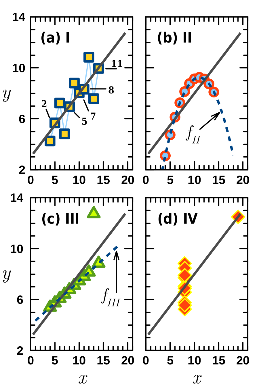
Anscombe’s original quartet, i.e., datasets I–IV, listed in Table 1, is visualized in Fig. 1, representing graphically distinct patterns of ’s with respect to . A brief analysis of the quartet is as follows. Fig. 1(a) shows an apparently linear trend of dataset I, typical in studies of various disciplines. Fig. 1(b) (of circular symbols) shows a parabolic, concave-down trend of , having its peak at . Most points in dataset I and II are closely located near the linear trend line. On the other hand, Fig. 1(c) has a noticeable outlier above a linear line that passes through the vicinity of the rest of the 10 points. Fig. 1(d) has a bimodal distribution of the 11 data points, i.e., a group of 10 points at one -coordinate and one outlier away from the group. Interestingly, the four datasets of the distinct patterns contain identical statistical properties, summarized in Table 2. In each dataset, the sample size is equally ; the mean and variance of are and , respectively; and those of are and , respectively. (In Anscombe’s original work, sums of and are reported, instead of variances, as 111.0 and 41.25, respectively.) The regression statistics provide the same values of , , and , with acceptable errors. To the best of our knowledge, how Anscombe generated the data quartet has not been well explained in the literature. Because our goal is to create multiple degenerate datasets of the same statistical properties, we here investigate the characteristics of Anscombe’s quartet data in detail.
For a better understanding, we first sorted the datasets in Table 1 in an ascending order of and made Table 3. Note that the sequences of data pairs do not change the statistical results of the linear regression. For example, even if the first two points of dataset I in Table 1, i.e., and , are exchanged to and , the regression statistics of , , and values remain invariant. In Table 3, it is noticed that datasets I–III have an evenly distributed from 4 to 14 with a fixed interval of 1, and the outliers () of datasets III and IV are located near the end of the regression line in . Now, we explain how the and vectors were possibly generated, keeping the statistical constraints discussed above.
| I | II | III | IV | |||
|---|---|---|---|---|---|---|
| Index | ||||||
| 1 | 10.0 | 8.04 | 9.14 | 7.46 | 8.0 | 6.58 |
| 2 | 8.0 | 6.95 | 8.14 | 6.77 | 8.0 | 5.76 |
| 3 | 13.0 | 7.58 | 8.74 | 12.74 | 8.0 | 7.71 |
| 4 | 9.0 | 8.81 | 8.77 | 7.11 | 8.0 | 8.84 |
| 5 | 11.0 | 8.33 | 9.26 | 7.81 | 8.0 | 8.47 |
| 6 | 14.0 | 9.96 | 8.10 | 8.84 | 8.0 | 7.04 |
| 7 | 6.0 | 7.24 | 6.13 | 6.08 | 8.0 | 5.25 |
| 8 | 4.0 | 4.26 | 3.10 | 5.39 | 19.0 | 12.50 |
| 9 | 12.0 | 10.84 | 9.13 | 8.15 | 8.0 | 5.56 |
| 10 | 7.0 | 4.82 | 7.26 | 6.42 | 8.0 | 7.91 |
| 11 | 5.0 | 5.68 | 4.74 | 5.73 | 8.0 | 6.89 |
| Index | Property | Value |
|---|---|---|
| 1 | The sample size | |
| 2 | The mean of | |
| 3 | The variance of | |
| 4 | The mean of | |
| 5 | The variance of | |
| 6 | The slope | |
| 7 | The intercept | |
| 8 | The coefficient of determination |
| I | II | III | IV | |||
|---|---|---|---|---|---|---|
| Index | ||||||
| 1 | 4.0 | 4.26 | 3.10 | 5.39 | 8.0 | 5.25 |
| 2 | 5.0 | 5.68 | 4.74 | 5.73 | 8.0 | 5.56 |
| 3 | 6.0 | 7.24 | 6.13 | 6.08 | 8.0 | 5.76 |
| 4 | 7.0 | 4.82 | 7.26 | 6.42 | 8.0 | 6.58 |
| 5 | 8.0 | 6.95 | 8.14 | 6.77 | 8.0 | 6.89 |
| 6 | 9.0 | 8.81 | 8.77 | 7.11 | 8.0 | 7.04 |
| 7 | 10.0 | 8.04 | 9.14 | 7.46 | 8.0 | 7.71 |
| 8 | 11.0 | 8.33 | 9.26 | 7.81 | 8.0 | 7.91 |
| 9 | 12.0 | 10.84 | 9.13 | 8.15 | 8.0 | 8.47 |
| 10 | 13.0 | 7.58 | 8.74 | 12.74 | 8.0 | 8.84 |
| 11 | 14.0 | 9.96 | 8.10 | 8.84 | 19.0 | 12.50 |
Constraints Applied
The 11 components of in dataset I–III can be represented as for with , so that the component is described as , and the mean of is calculated as
| (5) |
that provides for . Now, one can use a more flexible relationship between and by having an arbitrary interval , such as
| (6) |
and then the two parameters of and can be determined by preset constraints of and , such as
| (7) | |||||
| (8) |
where is an mid-point index. Here, we restrict ourselves to odd cases for simplicity. Substitution of , (obtained from ), and into Eqs. (7) and (8) results in and , as shown in Table 3. On the other hand, dataset IV has a special set of , containing only two values, denoted as and . Because the sequential indices of do not influence any statistical analysis, the mean of is written as
| (9) |
and further
| (10) |
where for . Anscombe used the fixed value of , which is represented below, using and , as
| (11) |
using Eq. (10). Finally, we obtain (for )
| (12) |
where the latter case of was chosen in Anscombe’s original work [6].
When a paired dataset is fitted on a straight line, the goodness of the linear regression is often estimated using the coefficient of determination of Eq. (3). Alternatively, the slope coefficient can be set as the last constraint, in addition to and , requiring the minimum sample size of to fully implement the six statistical constrains. In the next section, we discuss how to generate the three data points that hold the six statistical constrains.
A minimum data set of three components
| 1 | 5.6834 | 6.5187 | 5.1647 |
|---|---|---|---|
| 2 | 9.0000 | 6.1460 | 8.8540 |
| 3 | 12.3166 | 9.8353 | 8.4813 |
Let’s consider three consecutive values of , with the predetermined constraints of and , to have
| (13) |
where , , so that and . The following equations are obtained for of three components, such as
| (14) | |||||
| (15) | |||||
| (16) |
using and . Analytic solutions of for to are obtained as
| (17) | |||||
| (18) | |||||
| (19) |
where .
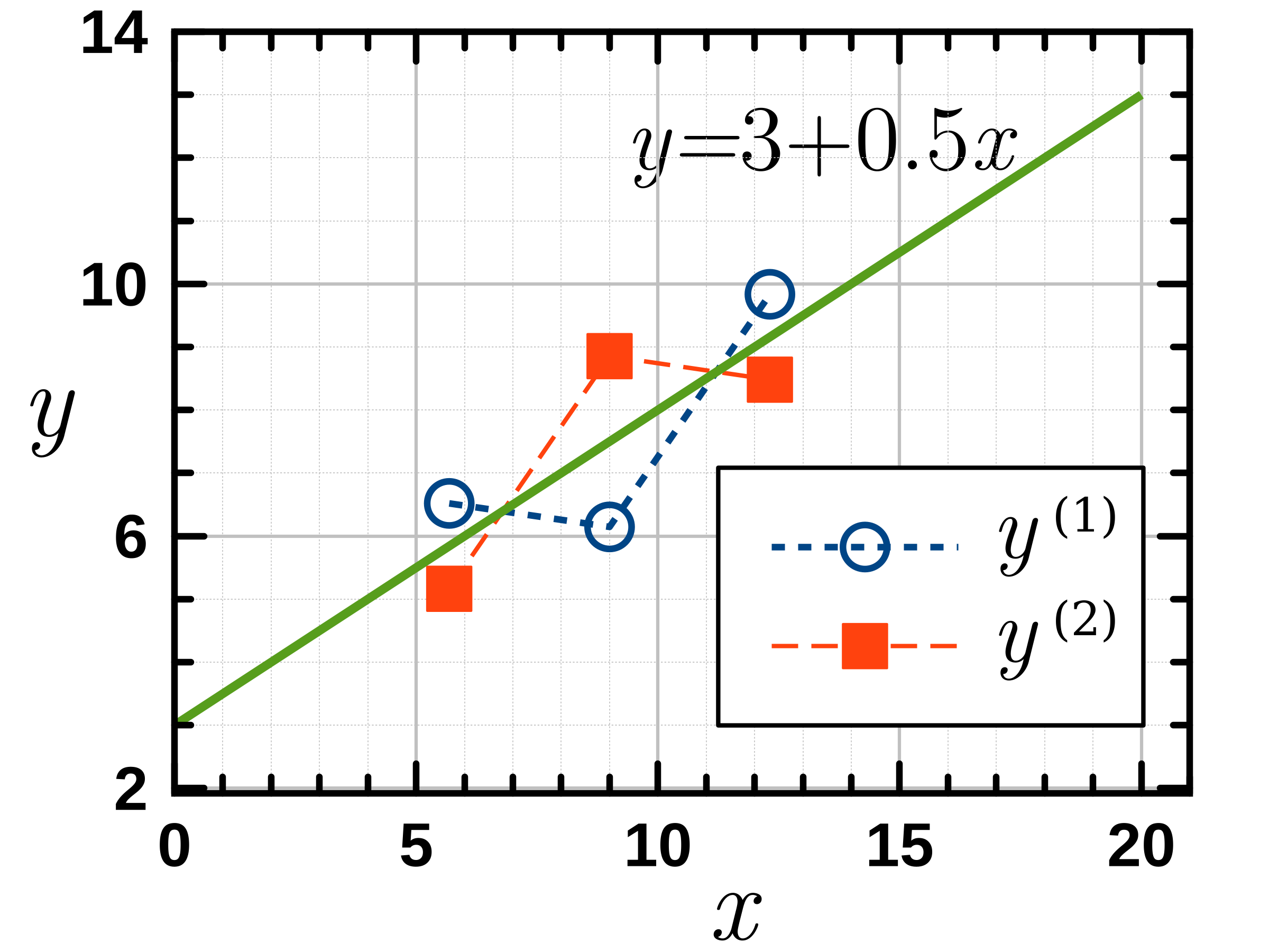
Table 4 shows two sets of solutions, denoted as and , while both satisfy all of the constraints indicated above. This degeneracy is due to the squared feature of the variance of Eq. (15). Fig. 2 shows the two sets of versus with , following the same Anscombe’s constraints, except for the sample size. Even with this smallest number of the sample size for a linear regression, two possible cases of degenerate ’s co-exist, having the identical statistical properties. A trivial case is that if , then and , so that and become identical, and so will be located on the regression line.
Generation of degenerate datasets with constraints
Satisfying three constraints using three arbitrary points
After the vector of a size of is determined with constraints of and , other three constraints should be satisfied by vector, which include finite and , alternately represented as
| (20) |
and
| (21) |
respectively; and finally, defined as a ratio of a covariance between and to a variance of , i.e., , such as
| (22) |
Because the vector is generated independently, all the constraints for an arbitrary are satisfied by the creation of the vector, having a degree of freedom of . In our approach, we generate an initial vector (as a function of the vector), having a specific pattern near the preset regression line of Eq. (2). Then we select the minimum, maximum, and mid-point of the vector and adjust the three values of the corresponding -components to satisfy the constraints of Eqs. (20)–(22). Assume that we already have a sorted vector, i.e., for , and have decided , except , , and , where is theoretically any index between 1 and , i.e., . For simplicity, an index of the mid-point can be used, such as
| (23) |
where is a remainder when is divided by 2, or simply
| (24) |
which is to round off , especially for odd . The above three equations can be rewritten as
| (25) | |||||
| (26) | |||||
| (27) |
where is defined as a summation over , except the first and last indices. Combining Eqs. (25) and (27), we represent and as linear functions of , such as
| (28) | |||||
| (29) |
where
| (30) | |||||
| (31) | |||||
| (32) | |||||
| (33) |
and substitute Eqs. (28) and (29) into (26) to derive for , such as
| (34) |
where
| (35) | |||||
| (36) | |||||
| (37) |
In this case, two sets of , and hence , are generated, depending on the sign of the square-root term in Eq. (34). Furthermore, there are no mandatory conditions that the first and last points should be included to meet the constraints. Instead, three arbitrary points within a dataset , e.g., , , and , can be selected as long as they are different, i.e., . Nevertheless, if the -positions of the three points are closely located, then large differences between their -values are expected.
Selection of a shape function
In previous sections, we discussed how to determine the components of the vector, especially three points, assuming that the rest points are already properly located near the given regression line of Eq. (2). The predetermination of points is to have the equal numbers of constraints (3) and unknown points (3). Because is also the degree of freedom of the pre-positioned values, the number of patterns that the elements of can make is theoretically infinite. In addition, having as one of the constraints doubles the degeneracy of the created dataset. Here, we consider a function that determines the initial distribution of points, among which , , and are updated to meet the three statistical constraints (, , and ). We name this function as a shape function and discuss how shape functions are used in Anscombe’s datasets in the following.
Random distribution
In Fig. 1(a) for dataset I, five points (of index 2, 5, 7, 8, and 11 in Table 3) are located very close to the regression line of : among the rest, half of them are above the regression line, and the other half are below it. The subset consisting of the closest five pairs of 2, 5, 7, 8, and 11 has a regression line of with . In this case, the shape function of dataset I is a linear line, similar to the predetermined regression line plus random biases, such as
| (38) |
where and is a random vector, having normally distributed random components with zero mean and a finite variance, denoted as . For dataset I, should consist of 11 components, selected from a population of normally distributed random numbers, with a mean of and standard deviation of .
Quadratic function
In Fig. 1(b), the parabolic pattern of dataset II is best fitted using a quadratic shape function
| (39) |
where is an -position at an extrema of and is a coefficient of the quadratic term. From Table 3, it is straightforward to find that . By trial and error, we found that with . In addition, the flipped (degenerate) shape function is obtained, such as
| (40) |
and plotted using star symbols. In this case, the three constants of , , and should be simultaneously determined to satisfy the three constraints. Eqs. (20), (21), and (22) are satisfied as follows:
| (41) | |||||
| (42) | |||||
| (43) |
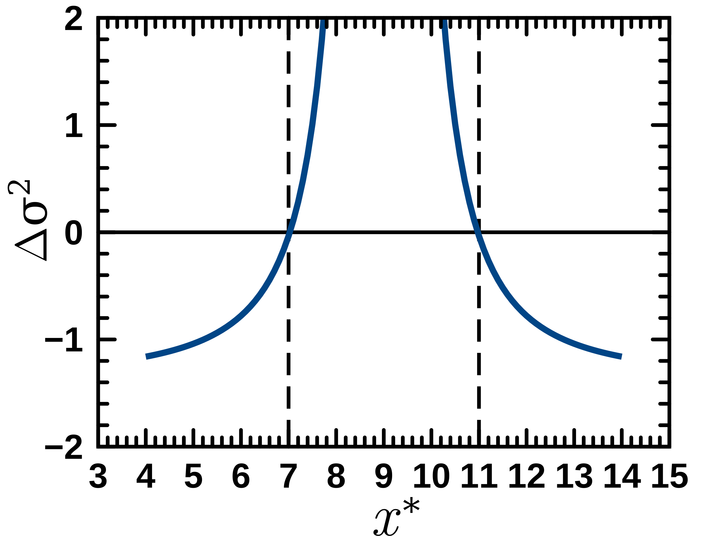
indicating that , , and as a function of , , and with the predetermined constraint . Therefore, can be obtained by plotting
| (44) |
with respect to and graphically finding of , as shown in Fig. 3. Here, and are calculated using Eqs. (41) and (42), respectively, using visually found . Similarly, for , we obtained and . These two parameter sets of , , and are used to plot and , shown in Fig. 1(b).
In Fig. 1(c), a subset of 10 points, excluding the outlier of , are aligned on a straight line, of which the regression line is calculated as
| (45) |
where , , and , which can be considered as a shape function of dataset III. Compared to the given regression line of Eq. (2), has a higher intercept and a gentler slope, as compared to those of Eq. (2), as well as of dataset I. A condition can be suggested, such as , so that if the slope is stiffer than , i.e., ; then the intercept is located below , and vice versa. After locating points on or near the linear shape function of Eq. (45), one arbitrary point, such as for in dataset III, can be made as an outlier by changing the value. In theory, relocating an outlier position cannot fully satisfy the three constraints. Instead, this outlier can be included as one of the three points used for the degenerate dataset’s creation by replacing the mid-point, i.e., . Furthermore, the first and last points can also be replaced by any two distinct points, if needed.
In Fig. 1(d) of dataset IV, a group of ten points is located at a same -positions, i.e., . These ten points have a mean of 7.0 and a variance of 1.527, which increased to the preset values of and , respectively, by including the outlier of that already satisfies . At , can be modeled as normally distributed random numbers of zero mean and finite variance , such as , similar to Eq. (38), such as
| (46) |
Because the last point is fixed, any three points at should be (randomly) selected and updated to meet the given constraints.
General algorithm
If a paired dataset shows a monotonous variation of with respect to , or vice versa, then the above-mentioned algorithms can be generalized and used to create degenerate datasets of the same constrains, as follows
-
1.
determine six statistical parameters: , , , , and and calculate ;
-
2.
make an vector of components, having predetermined and ;
-
3.
use a shape function to initialize -components near the given regression line, , of Eq. (2);
- 4.
-
5.
confirm that the generated dataset is characterized by the six parameters listed above.
In general, when constraints are implemented, points are determined using a shape function, and the rest of the points can be determined by analytically solving the constraint equations. The availability of analytic solutions will be limited as the number of constraints increases. In this case, the problem can be described as a linear regression with constraint functions of
| (47) |
where is one of components of , chosen to satisfy constraints. A general root-finding algorithm can be used to numerically find .
III Results and Discussions
Inverse Sampling of Degenerate Datasets
The creation of one of degenerate paired datasets requires six constraints, such as , , , , and . For a given sample size , the mean and standard deviation of and determine their central locations and spread degrees. If more than three constraints are considered, the degrees of degeneracy are theoretically infinite, and therefore, one can create as many as degenerate datasets as needed, disregarding their graphical similarities or dissimilarities. If a trend line is made by a linear regression of multiple datasets of the same size, then it is highly probable that the degenerate datasets created from the calculated trend line do not include the original datasets used for the linear regression, but instead can include unexpected forms of meaningful datasets.
In statistical physics, the importance sampling technique is frequently used for efficient Monte Carlo simulations [18, 19], which indicates sampling from only specific distributions that over-weigh the important region. In a microcanonical ensemble of a thermodynamic system, sampling of particles’ positions and velocities are under a constant total energy [20]. Once particle positions are determined, a specific value of kinetic energy is calculated as the total energy subtracted by the position-dependent potential energy, such as , and particle velocities are randomly assigned and carefully adjusted to maintain the kinetic energy. There are many distinct configurations of velocities in the phase space that give the same kinetic energy value. This specific sampling is called inverse sampling, which is analogous to the present work that inversely calculates and samples datasets of specific statistical constraints.
Paired datasets generated using shape functions
In this section, we create a few paired datasets having the same statistical properties of Anscombe’s quartet. A test shape function we employed is a fourth-order polynomial with respect to , such as
| (48) |
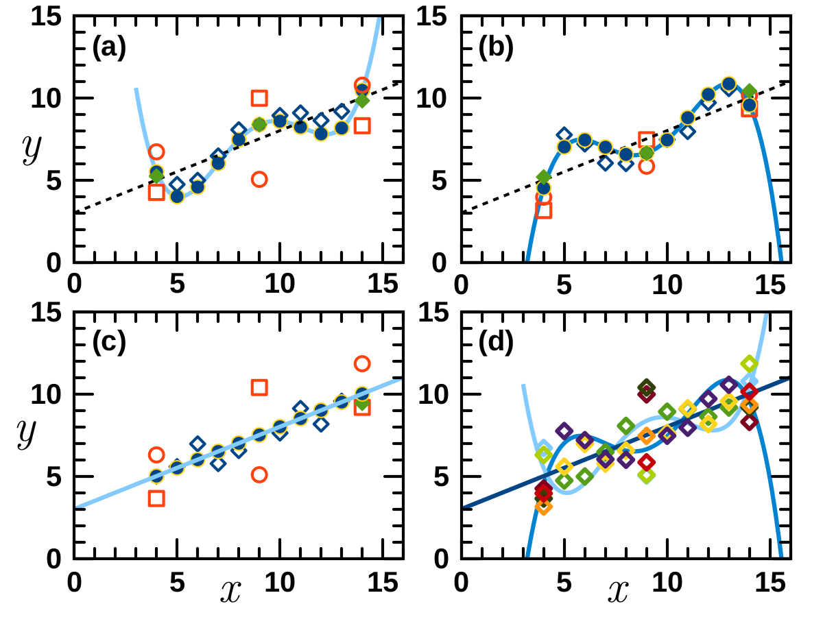
where , , , and are chosen slightly away from the (integer) value; and is a weight factor of the shape function, which is either 0 or . The non-zero magnitude of is selected by trial and error. If .0, then the predetermined regression line becomes the shape function itself. Linear regressions using the shape function are summarized in Fig. 4, as discussed below.
-
1.
These shape functions of positive, negative, and zero values are made and shown in Fig. 4(a), (b), and (c), respectively. Figs. 4(a) and (b) show smooth shape functions with opposite signs, and Fig. 4(c) shows the predetermined linear regression line as the shape function so that initial points are located on the regression line. Fig. 4(d) combines all the datasets and shape functions, generated in (a)–(c), and shows the overall trend.
-
2.
In each of Figs. 4(a)–(c), points initially on the shape function (filled circles) are randomly relocated to new neighboring positions (hollow diamonds) above or below the original positions.
-
3.
Three vertical positions of for , , and are adjusted to two distinct groups (hollow circles and rectangles), of which both satisfy the given constraints using the algorithm discussed above.
Since there are, in principle, an infinite number of available shape functions and multiple ways to locate data points near the shape functionss, identifying data patterns seems to be challenging work, even if the trend seems to follow a noticeable shape. Nevertheless, this work provides in-depth analysis of Anscombe’s original work in terms of data creation, and a straightforward algorithm to reproduce his work, as well as to perform the inverse sampling of regressible datasets.
Further Considerations
While is predetermined independently, the three effective constraints provide the same number of closure equations, reducing the degrees of freedom of from to . It is worth noting that the degeneracy is originated not only by the number of elements, but also from the squared form of , i.e., the expected value of or the second central moment. Even if we have only three points (), two datasets are generated due to the intrinsic degenerate characteristics of the variance, as previously shown in Fig. 2. After points are decided for a paired sample of , there are still two degrees of degeneracy, due to the squared feature of variances.
In addition to the three constraints discussed above, one can include more constraints, such as, but not limited to, the least magnitude (instead of squared) of errors, linear regression with perpendicular offsets [21], heteroscedasticity [22], Kolmogorov-Smirnov statistic[1], Lagrange multiplier (LM) statistic [22], standardized skewness, standardized Kurtosis, and D-statistic[9]. Each of these statistics can be used as an additional constraint to quantitatively identify statistical similarities. Adding or replacing some of the above-mentioned constraints to the standard constraints will create too many distinct datasets to visually compare. However, if the created datasets are tested for various indices, they can easily be classified in to several groups of similarities [23].
Table 5 shows the third and fourth moments of the -scores of and , denoted as and , respectively. The moment of is defined as a mean value of , i.e., , and the third and fourth moments are called standard skewness and kurtosis, respectively. Because the ’s of datasets I–III are equally evenly distributed, their mean, variance, skewness, and kurtosis are identical, which is not observed in dataset IV. The -skewness of dataset I and II have negative values, indicating that more -values are located below . The larger magnitude of than indicates the quadratic shape function of dataset II locates more data points lower than the regression line than those of dataset I. The two largest -skewnesses of dataset III and IV are ascribed to their outliers. The -kurtosis values of the four datasets show a similar trend to those of skewnesses, and the -Kurtosis values increase from dataset I to dataset IV, also following the similar trend of absolute -skewnesses. Including higher order moments will require the same number of additional constraints to make multiple datasets statistically identical within the range of constraints applied.
| Dataset | ||||
|---|---|---|---|---|
| I | 0.000 | 1.471 | 0.048 | 1.801 |
| II | 0.000 | 1.471 | 0.979 | 2.486 |
| III | 0.000 | 1.471 | 1.377 | 4.228 |
| IV | 2.467 | 7.521 | 1.119 | 3.622 |
IV Conclusion
Testing the similarities or identicalness of two datasets from distinct origins is an ubiquitously important issue in statistics, applicable to various studies. When a paired dataset is linearly regressed, the trend line indicates correlation degrees of how the response variable depends on the independent variable , assuming that one is a cause and the other is an effect, or vice versa. In reality, it is rare to have two or more visually different datasets that provide an identical regression equation. On the other hand, a given regression equation can interpret or explain a number of datasets from various sources. Here, we recognized that a robust method to sample many degenerate datasets satisfying the given constraints is of great necessity, not only in advanced data sciences and applications, but also in applied statistics education at college and graduate levels. In this work, we presented an algorithm to sample many degenerate datasets having the identical six constraints used for a linear regression. Our method is extendable for an arbitrary number of constraints, including higher-order statistical moments, to create statistically closer datasets.
References
- [1] Frank J. Massey. The Kolmogorov-Smirnov Test for Goodness of Fit. Journal of the American Statistical Association, 46(253):68–78, 1951.
- [2] Francis Galton. Kinship and Correlation. Statistical Science, 4(2):419–431, 1989.
- [3] Peter J. Ireland, Andrew D. Bragg, and Lance R. Collins. The Effect of Reynolds Number on Inertial Particle Dynamics in Isotropic Turbulence. Part 2. Simulations with Gravitational Effects. Journal of Fluid Mechanics, 796:659–711, 2016.
- [4] G. Udny Yule. On the Theory of Correlation. Journal of the Royal Statistical Society, 60(4):812–854, 1897.
- [5] Karl Pearson. The Law Of Ancestral Heredity. Biometrika, 2(2):211–228, 1903.
- [6] F. J. Anscombe. Graphs in Statistical Analysis. The American Statistician, 27(1):17–21, 1973.
- [7] R. Dennis Cook and Sanford Weisberg. Graphs in Statistical Analysis: Is the Medium the Message? The American Statistician, 53(1):29–37, 1999.
- [8] Guillaume A. Rousselet, Cyril R. Pernet, and Rand R. Wilcox. Beyond differences in means: robust graphical methods to compare two groups in neuroscience. European Journal of Neuroscience, 46(2):1738–1748, 2017.
- [9] R. Dennis Cook. Detection of Influential Observation in Linear Regression. Technometrics, 19(1):15–18, 1977.
- [10] Lori L. Murray and John G. Wilson. Generating data sets for teaching the importance of regression analysis. Decision Sciences Journal of Innovative Education, 19(2):157–166, 2021.
- [11] Edward Schneider and Corey Dineen. Adding a dimension to Anscombe’s quartet: Open source, 3-D data visualization: Adding a Dimension to Anscombe’s Quartet: Open Source, 3-D Data Visualization. Proceedings of the American Society for Information Science and Technology, 50(1):1–3, 2013.
- [12] Reginald Smith. A mutual information approach to calculating nonlinearity. Stat, 4(1):291–303, 2015.
- [13] Ahmad Hosseinzadeh, Mansour Baziar, Hossein Alidadi, John L. Zhou, Ali Altaee, Ali Asghar Najafpoor, and Salman Jafarpour. Application of artificial neural network and multiple linear regression in modeling nutrient recovery in vermicompost under different conditions. Bioresource Technology, 303:122926, 2020.
- [14] Faezehossadat Khademi, Mahmoud Akbari, Sayed Mohammadmehdi Jamal, and Mehdi Nikoo. Multiple linear regression, artificial neural network, and fuzzy logic prediction of 28 days compressive strength of concrete. Frontiers of Structural and Civil Engineering, 11(1):90–99, 2017.
- [15] C. L. Lin, J. F. Wang, C. Y. Chen, C. W. Chen, and C. W. Yen. Improving the generalization performance of RBF neural networks using a linear regression technique. Expert Systems with Applications, 36(10):12049–12053, 2009.
- [16] Noam Shoresh and Bang Wong. Data exploration. Nature Methods, 9(1):5–5, 2012.
- [17] Max Halperin. On Inverse Estimation in Linear Regression. Technometrics, 12(4):727–736, 1970.
- [18] Michael P. Allen and Dominic J. Tildesley. Computer Simulation of Liquids, volume 1. Oxford University Press, 2017.
- [19] Jim C. Chen and Albert S. Kim. Monte Carlo Simulation of Colloidal Membrane Filtration: Principal Issues for Modeling. Advances in Colloid and Interface Science, 119(1):35–53, 2006.
- [20] Harold W. Schranz, Sture Nordholm, and Gunnar Nyman. An efficient microcanonical sampling procedure for molecular systems. The Journal of Chemical Physics, 94(2):1487–1498, 1991.
- [21] Jorge H. B. Sampaio. An iterative procedure for perpendicular offsets linear least squares fitting with extension to multiple linear regression. Applied Mathematics and Computation, 176(1):91–98, 2006.
- [22] T. S. Breusch and A. R. Pagan. A Simple Test for Heteroscedasticity and Random Coefficient Variation. Econometrica, 47(5):1287, 1979.
- [23] Xavier X. Sala-I-Martin. I Just Ran Two Million Regressions. The American Economic Review, 87(2):178–183, 1997.