Optical solitons and vortices in fractional media: A mini-review of recent results

Abstract

The article produces a brief review of some recent results which predict stable propagation of solitons and solitary vortices in models based on the nonlinear Schrödinger equation (NLSE) including fractional one- or two-dimensional diffraction and cubic or cubic-quintic nonlinear terms, as well as linear potentials. The fractional diffraction is represented by fractional-order spatial derivatives of the Riesz type, defined in terms of the direct and inverse Fourier transform. In this form, it can be realized by spatial-domain light propagation in optical setups with a specially devised combination of mirrors, lenses, and phase masks. The results presented in the article were chiefly obtained in a numerical form. Some analytical findings are included too – in particular, for fast moving solitons, and results produced by the variational approximation. Also briefly considered are dissipative solitons which are governed by the fractional complex Ginzburg-Landau equation.

Keywords: fractional diffraction; Riesz derivative; nonlinear Schrödinger equations; soliton stability; Vakhitov–Kolokolov criterion; collapse; symmetry breaking; complex Ginzburg–Landau equations; vortex necklaces; dissipative solitons

I Introduction and the basic models

Nonlinear Schrödinger equations (NLSEs) give rise to soliton families in a great number of realizations [1]-[8], many of which originate in optics. The introduction of fractional calculus in NLSEs has drawn much interest since it was proposed – originally, in the linear form – as the quantum-mechanical model, derived from the respective Feynman-integral formulation, for particles moving by Lévy flights [9, 10]. Experimental implementation of fractional linear Schrödinger equations has been reported in condensed matter [11, 12] and photonics [13], in the form of transverse dynamics in optical cavities. Realization of the propagation dynamics of light beams governed by this equation was proposed in Ref. [14], followed by its extension for models including complex potentials subject to the condition of the parity-time ($\mathcal{PT}$) symmetry [15, 16]. Generally, optical settings modeled by linear and nonlinear fractional Schrödinger equations may be considered as a specific form of artificial photonic media.

The modulational instability of continuous waves [17] and many types of optical solitons produced by fractional NLSEs [18]-[48] have been theoretically investigated, chiefly by means of numerical methods. These are quasi-linear “accessible solitons” (actually, quasi-linear modes) [20, 21], gap solitons supported by spatially periodic (lattice) potentials [26]-[30], solitary vortices [31, 32], multipole and multi-peak solitons [33]-[36], soliton clusters [37], solitary states with spontaneously broken symmetry [40, 41, 42], as well as solitons in optical couplers [43, 44]. Dissipative solitons in fractional complex Ginzburg-Landau equation (CGLE) were studied too [39].

The objective of this article is to present a short review of models based on fractional NLSEs and some states produced by them. The review is not drafted to be a comprehensive one, the bibliography not being comprehensive either; rather, it selects several recent results which seem interesting in terms of the general soliton dynamics.

The basic form of the one-dimensional (1D) fractional NLSE model, written for amplitude $\Psi$ of the optical field, is

$$i\frac{\partial\Psi}{\partial z}=\frac{1}{2}\left(-\frac{\partial^{2}}{\partial x^{2}}\right)^{\alpha/2}\Psi+V(x)\Psi-g\left|\Psi\right|^{2}\Psi.$$ (1)

Here $z$ and $x$ are the scaled propagation distance and transverse coordinate, $g>0$ ($g<0$) is the coefficient representing the self-focusing (defocusing) cubic (Kerr) nonlinearity, and $V(x)$ is a trapping potential which may be included in the model. The fractional-diffraction operator with the Lévy index $\alpha$ (in the original fractional Schrödinger equation, it characterizes the hopping motion of the quantum particle [9]) is defined, in the form of the Riesz derivative [45], by means of the juxtaposition of the direct and inverse Fourier transform [9]-[13], [19]:

$$\left(-\frac{\partial^{2}}{\partial x^{2}}\right)^{\alpha/2}\Psi=\frac{1}{2\pi}\int_{-\infty}^{+\infty}dp|p|^{\alpha}\int_{-\infty}^{+\infty}d\xi e^{ip(x-\xi)}\Psi(\xi),$$ (2)

In particular, the above-mentioned concatenation of mirrors, lenses, and phase masks in optical cavities makes it possible to implement the effective fractional diffraction approximated by operator (2) [13].

The Lévy index in Eq. (1) may take values

$$1<\alpha\leq 2,$$ (3)

where $\alpha=2$ corresponds to the normal paraxial diffraction, represented by operator $-\partial^{2}/\partial x^{2}$. Equation (1) with $g>0$ (self-focusing) gives rise to the critical collapse at $\alpha=1$ (and to the supercritical collapse at $\alpha<1$), which destabilizes all possible soliton solutions [23, 39], therefore only values $\alpha>1$ are usually considered (the linear fractional Schrödinger equation with $\alpha=1$ admits analytical solutions based on Airy functions [13]).

In the case of quadratic self-focusing nonlinearity, the critical collapse occurs at $\alpha=1/2$, hence the Lévy index may take values $1/2<\alpha\leq 2$ in that case. The quadratic self-focusing term appears on the right-hand side of Eq. (1), in the form of $-\varepsilon|\psi|\psi$ with $\varepsilon>0$, as the correction induced by quantum fluctuations [46] to the 1D fractional Gross-Pitaevskii equation for the gas of Lévy-hopping particles [47].

Besides the real waveguiding potential, $V(x)$, Eq. (1) may include a $\mathcal{PT}$-symmetric complex potential, with even real and odd imaginary parts:

$$V^{\ast}(x)=V(-x),$$ (4)

where $\ast$ stands for the complex conjugate. As usual, in terms of optical waveguides the odd imaginary part of potential (4) represents spatially separated and mutually balanced gain and loss elements.

The two-dimensional (2D) version of the underlying equation (1), with two transverse coordinates, $x$ and $y$, is written as

$$i\frac{\partial\Psi}{\partial z}=\frac{1}{2}\left(-\frac{\partial^{2}}{\partial x^{2}}-\frac{\partial^{2}}{\partial y^{2}}\right)^{\alpha/2}\Psi+V(x,y)\Psi-g\left|\Psi\right|^{2}\Psi.$$ (5)

In this case, the fractional-diffraction operator is defined as

$$\left(-\frac{\partial^{2}}{\partial x^{2}}-\frac{\partial^{2}}{\partial y^{2}}\right)^{\alpha/2}\Psi=\frac{1}{(2\pi)^{2}}\int\int dpdq\left(p^{2}+q^{2}\right)^{\alpha/2}\int\int d\xi d\eta e^{i\left[p(x-\xi)+iq(y-\eta)\right]}\Psi(\xi,\eta),$$ (6)

cf. Eq. (2).

The rest of the article is organized as follows. In Section II, basic numerical and analytical results are presented for soliton families generated by the 1D fractional NLSE (1) in the free space (without the trapping potential, $V=0$). Other essential numerical findings for 1D solitons are presented in Section III. In particular, these are results produced by trapping potentials, and dissipative solitons obtained in the framework of the fractional complex Ginzburg-Landau equation (CGLE) with the cubic-quintic nonlinearity. Selected results for 2D solitons, including ones with embedded vorticity and necklace-shaped soliton clusters, are collected in Section IV. To secure stability of the solitons, the 2D model includes the quintic self-defocusing term, in addition to the cubic self-focusing one; the stabilization of 2D solitons can also be provided by the parabolic trapping potential, see Eqs. (47) and (55) below. The paper is concluded by Section V.

II Basic soliton families in the one-dimensional fractional medium

II.1 Stationary states and analysis of their stability

Steady-state solutions to Eq. (1) with propagation constant $-\mu$ are looked for in the form of

$$\Psi(x,z)=U(x)\mathrm{exp}(-i\mu z),$$ (7)

with real function $U(x)$ satisfying the stationary equation,

$$\mu U=\frac{1}{2}\left(-\frac{\partial^{2}}{\partial x^{2}}\right)^{\alpha/2}U-gU^{3}$$ (8)

(here, the external potential is dropped, $V=0$). The stationary states are characterized by their power (alias norm),

$$N=\int_{-\infty}^{+\infty}\left|U(x)\right|^{2}dx.$$ (9)

Stability of these states was investigated by taking the perturbed solution as

$$\Psi=[U(x)+a(x)\mathrm{exp}(\lambda z)+b^{\ast}(x)\mathrm{exp}(\lambda^{\ast}z)]\mathrm{exp}(-i\mu z),$$ (10)

where $a(x)$ and $b^{\ast}(x)$ are components of small complex perturbations, and $\lambda$ is an instability growth rate (which may be complex). Substituting this ansatz in Eq. (1), one derives the linearized equations for $a$ and $b$:

$$i\lambda a = \frac{1}{2}\left(-\frac{\partial^{2}}{\partial x^{2}}\right)^{\alpha/2}a-\mu a+gU^{2}(2a+b),$$

$$i\lambda b = -\frac{1}{2}\left(-\frac{\partial^{2}}{\partial x^{2}}\right)^{\alpha/2}b+\mu b-gU^{2}(2b+a).$$ (11)

The underlying stationary solution (7) is stable provided that all eigenvalues $\lambda$ produced by Eq. (11) have zero real parts.

II.2 The quasi-local approximation for modes carried by a rapidly oscillating continuous wave

To better understand the purport of the fractional-diffraction operator defined by Eq. (2), it is instructive to consider its action on function $\Psi(x)$ built as a slowly varying envelope $\psi(x)$ multiplying a rapidly oscillating continuous-wave carrier,

$$\Psi\left(x\right)=\psi(x)e^{iPx},$$ (12)

with large wavenumber $P$. In particular, this ansatz may be used to construct solutions for rapidly moving modes, see Eq. (15) below (in fact, in the spatial domain the “moving” modes are ones tilted in the $\left(x,z\right)$ plane). The substitution of wave form (12) in the nonlocal expression on the right-hand side of Eq. (2) readily leads to the following result, in the form of a quasi-local expression expanded in powers of small parameter $1/P$:

$$\left(-\frac{\partial^{2}}{\partial x^{2}}\right)^{\alpha/2}\left(\psi(x)e^{iPx}\right)=e^{iPx}|P|^{\alpha}\left[\psi+\sum_{n=1}^{\infty}(-i)^{n}\frac{\alpha\left(\alpha-1\right)...\left(\alpha-n+1\right)}{n!P^{n}}\frac{\partial^{n}\psi}{\partial x^{n}}\right].$$ (13)

The substitution of expansion (13), truncated at some $n=n_{\max}$, in Eq. (1) and cancellation of the common factor $e^{iPx}$ leads to the familiar NLSE with higher-order dispersion (diffraction) terms, which correspond to $n\geq 3$ in Eq. (13). In particular, setting $\psi=\mathrm{const}$ demonstrates that the dispersion relation produced by the linearized version of Eq. (8) is

$$\mu=(1/2)|P|^{\alpha},$$ (14)

in agreement with the analysis of Laskin [10]. Equation (14) implies that the semi-infinite bandgap, with $\mu<0$, may be populated by solitons, in the framework of the nonlinear equation.

As concerns the term $\sim i\partial\psi/\partial x$, corresponding to $n=1$, which appears after the substitution of expansion (13) in Eq. (1), it suggests one to rewrite the NLSE in the reference frame moving with the group velocity

$$V_{\mathrm{gr}}=\left(\alpha/2\right)|P|^{\alpha-1}\mathrm{sgn}(P),$$ (15)

i.e., to replace $x$ by

$$\tilde{x}\equiv x-V_{\mathrm{gr}}z$$ (16)

in the resulting equation (in fact, the group velocity is the tilt of spatial solitons). Note that, for values of the Lévy index belonging to interval (3), the group velocity is large for large $P$, while the effective second-order diffraction coefficient, as determined by the term with $n=2$ in Eq. (13), is small,

$$D_{2}=(1/2)\alpha\left(\alpha-1\right)|P|^{-\left(2-\alpha\right)}.$$ (17)

The respectively transformed NLSE (1) (without the external potential, $V(x)=0$), truncated at $n_{\max}=2$, is

$$i\frac{\partial\tilde{\psi}}{\partial z}=-\frac{1}{2}D_{2}\frac{\partial^{2}\tilde{\psi}}{\partial\tilde{x}^{2}}-g\left|\tilde{\psi}\right|^{2}\tilde{\psi},$$ (18)

where $\tilde{\psi}\left(\tilde{x},z\right)=\exp\left((i/2)|P|^{\alpha}z\right)\cdot\psi\left(x,z\right)$. The obvious soliton solution of Eq. (18) with the self-focusing nonlinearity, $g>0$, written in terms of norm (9), is

$$\tilde{\psi}=\exp\left(i\frac{(gN)^{2}}{8D_{2}}z\right)\frac{N}{2}\sqrt{\frac{g}{D_{2}}}\mathrm{sech}\left(\frac{N}{2}\frac{g}{D_{2}}\tilde{x}\right).$$ (19)

It follows from Eq. (17) that this soliton is a narrow one, with the width estimated as $W\sim N^{-1}|P|^{-\left(2-\alpha\right)}$. Further, in this case the terms representing higher-order diffraction terms with $n\geq 3$, which originate from the expansion (13), are relatively small perturbations decaying $\sim|P|^{-n\left(\alpha-1\right)}$.

II.3 The scaling relation and variational approximation (VA) for soliton families

Equation (8) gives rise to an exact scaling relation between the soliton’s power and propagation constant:

$$N(\mu,g)=N_{0}(\alpha)g^{-1}\left(-\mu\right)^{1-1/\alpha},$$ (20)

with a constant $N_{0}(\alpha)$ (its particular value is $N_{0}(\alpha=2)=2\sqrt{2}$, see Eq. (31) below). The fact that relation (20) satisfies the commonly known Vakhitov-Kolokolov (VK) criterion,

$$dN/d\mu<0$$ (21)

[49, 50] at $\alpha>1$ suggests that the respective soliton family may be stable, see further details in Fig. 3 below. The case of $\alpha=1$, which corresponds to the degenerate form of relation (20), with $N(\mu)\equiv\mathrm{const}$, implies the occurrence of the above-mentioned critical collapse, which makes all solitons unstable (cf. the commonly known cubic NLSE in the 2D space with the normal diffraction, $\alpha=2$, in which the family of Townes solitons, destabilized by the critical collapse, has a single value of the norm [50]). In the case of $\alpha<1$, the solitons generated by Eq. (8) are made strongly unstable by the presence of the supercritical collapse, similar to solitons of the usual cubic NLSE in three dimensions [50].

Localized solutions of the fractional NLSE can be looked for in an approximate analytical form by means of the variational approximation (VA) [23, 39, 51]. To introduce it, note that Eq. (8) for real $U(x)$, with the fractional diffraction operator defined as per Eq. (2), can be derived from the Lagrangian,

$$L=-\frac{\mu}{2}\int_{-\infty}^{+\infty}dxU^{2}(x)+\frac{1}{8\pi}\int_{-\infty}^{+\infty}dp|p|^{\alpha}\int\int d\xi dxe^{ip(x-\xi)}U(x)U(\xi)$$

$$-\frac{g}{4}\int_{-\infty}^{+\infty}dxU^{4}(x).$$ (22)

The simplest form of the variational ansatz approximating the solitons sought for is based on the Gaussian (cf. Ref. [53]),

$$\mathcal{U}(x)=A\exp\left(-\frac{x^{2}}{2W^{2}}\right),$$ (23)

with real amplitude $A$, width $W$, and the power calculated as per Eq. (9),

$$\mathcal{N}=\sqrt{\pi}A^{2}W$$ (24)

(the calligraphic font denotes quantities pertaining to VA). The substitution of the ansatz in Lagrangian (22) yields the corresponding effective Lagrangian, which may be conveniently written with squared amplitude $A^{2}$ replaced by the norm, according to Eq. (24) [39]:

$$L_{\mathrm{eff}}=-\frac{\mu}{2}\mathcal{N}+\frac{\Gamma\left(\left(1+\alpha\right)/2\right)}{4\sqrt{\pi}}\frac{\mathcal{N}}{W^{\alpha}}-\frac{g}{4\sqrt{2\pi}}\frac{\mathcal{N}^{2}}{W},$$ (25)

where $\Gamma$ is the Gamma-function. Then, values of $\mathcal{N}$ and $W$ are predicted by the Euler-Lagrange equations,

$$\partial L_{\mathrm{eff}}/\partial\mathcal{N}=\partial L_{\mathrm{eff}}/\partial W=0.$$ (26)

Particular examples of the solitons shapes predicted by the VA, and their comparison to the numerically found counterparts are shown in Fig. 1. At a fixed value of the Lévy index, soliton families are characterized by dependences $N(\mu)$. An example of such a VA-predicted dependence and its numerical counterpart are displayed in Fig. 2 for $\alpha=1.5$, which demonstrates a sufficiently good accuracy of the VA.

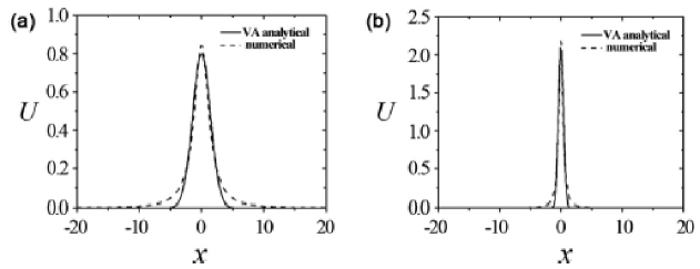
Figure 1: Profiles of solitons with $\mu=-0.3$ (a) and $-2.0$ (b), predicted by the VA based on the Gaussian ansatz  (23) and Euler-Lagrange equations (26), and their counterparts produced by the numerical solution of Eq. (8) with Lévy index $\alpha=1.5$ and $g=1$. Reprinted with permission from Ref. [39]. Copyright 2020 Elsevier.

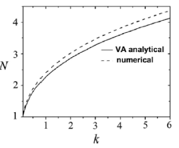
Figure 2: Dependence of the soliton’s norm $N$ on the propagation constant, $k\equiv-\mu$, for the Lévy index $\alpha=1.5$ and self-focusing coefficient $g=1$, as predicted by the VA based on the Gaussian ansatz  (23) and Euler-Lagrange equations (26). The corresponding dependence obtained from the numerical solution of Eq. (8) is included too. Reprinted with permission from Ref. [39]. Copyright 2020 Elsevier.

An essential result of the VA is the prediction of the fixed norm for the quasi-Townes solitons, for which the critical collapse takes place in the free space at $\alpha=1$ [39]:

$$\left(\mathcal{N}_{\mathrm{Townes}}\right)_{\mathrm{VA}}=\sqrt{2}\approx 1.41.$$ (27)

This result is similar to the well-known VA prediction for the norm of the Townes solitons in the 2D NLSE with the cubic self-focusing [53],

$$\left(\mathcal{N}_{\mathrm{Townes}}^{\mathrm{(2D)}}\right)_{\mathrm{VA}}=2\pi$$ (28)

[53], while the respective numerical value is

$$N_{\mathrm{Townes}}^{\mathrm{(2D)}}\approx 5.85$$ (29)

[50], the relative error of the VA being $\approx 7\%$. It is shown below in Fig. 3(c) that the numerically found counterpart of the variational value (27) is

$$\left(N_{\mathrm{Townes}}\right)_{\mathrm{num}}\approx 1.23.$$ (30)

Thus, the relative error of the VA prediction (27) is $\approx 13\%$. A relatively large size of the error is a consequence of the complicated structure of the equation with the fractional diffraction, especially for values of $\alpha$ which are taken far from the normal-diffraction limit, $\alpha=2$.

The VA also makes it possible to predict if dependence $N(\alpha)$ for a fixed value of $\mu$ is growing or decaying. To make this conclusion, one should take into account that, at $\alpha=2$, the usual NLSE with the cubic nonlinearity gives rise to the following $N(\mu)$ dependences for the commonly known soliton solutions:

$$N_{\alpha=2}=2\sqrt{-2\mu}.$$ (31)

Comparing it with the variational value (27), one concludes that the $N(\alpha)$ dependence is growing at $-\mu>-\mu_{\mathrm{crit}}\approx 1/4$, and decaying at $-\mu<-\mu_{\mathrm{crit}}$. This prediction agrees with numerical results displayed below in Fig. 3(c).

II.4 Numerical findings

Generic numerically obtained results for soliton families produced by Eqs. (1) and (8) are displayed in Figs. 3 and 4. The families are characterized by the dependence of the integral power $N$, defined as per Eq. (9), on the propagation constant $-\mu$ for fixed values of Lévy index $\alpha$, see a characteristic example for $\alpha=1.1$ in Fig. 3(a). Note that this value of $\alpha$ is taken far from the normal-diffraction limit, $\alpha=2$, and close to the collapse boundary, $\alpha=1$, in order to demonstrate the setting in which the fractional character of the diffraction is essential. It is seen that the numerically computed dependence exactly follows the analytical prediction given by Eq. (20), with a properly fitted constant $N_{0}(\alpha)$. Blue and red segments in the $N(\mu)$ curve identify, respectively, stable and unstable soliton subfamilies.

Further, a curve representing a typical dependence $N(\alpha)$ for a fixed propagation constant, $-\mu=1.5$, which is also split in stable and unstable segments, is exhibited in Fig. 3(c). Unlike the $N(\mu)$ dependence, this one cannot be predicted in an exact analytical form. Nevertheless, as mentioned above, the VA based on ansatz (23) predicts the approximate value given by Eq. (27) for the degenerate ($\mu$-independent) norm of the quasi-Townes solitons at $\alpha=1$, which is close enough to its numerical counterpart (30). At $\alpha=2$, the numerical value $N_{\mathrm{numer}}\left(\mu=1.5,\alpha=2\right)\approx 3.46$ is in complete agreement with the exact analytical value given by Eq. (31) (it is $N(\mu=-1.5)=2\sqrt{3}$).

Typical profiles of the solitons with different values of $\mu$ and $\alpha$, taken at points labeled B1–B4 in Figs. 3(a) and (c), are presented in Figs. 3(b,d), respectively. In particular, the trend of the solitons to get narrower with the increase of $|\mu|$ is another manifestation of the scaling expressed by Eq. (20).

Stable and unstable perturbed propagation of the solitons whose stationary shapes are shown in Figs. 3(b,d) is displayed in Fig. 4. It is seen that, if the solitons are unstable, dynamical manifestations of the instability are quite weak, in the form of spontaneously developing small-amplitude intrinsic vibrations of the solitons. The instability of the solitons belonging to the red segments of the $N(\mu)$ and $N(\alpha)$ dependences in Figs. 3(a) and (c) is always accounted for by a pair of real eigenvalues $\pm\lambda$ produced by numerical solution of Eqs. (11).

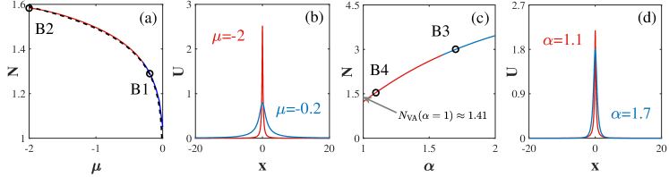
Figure 3: (a) Dependence $N(\mu)$ and (b) profiles of solitons labeled B1 and B2 in (a) (corresponding to $\mu=-0.2$ and $-2$, respectively), as produced by numerical solution of Eq. (8) in the free space ($V=0$), for a fixed value of the Lévy index, $\alpha=1.1$, and nonlinearity coefficient, $g=1$. (c) Dependence $N(\alpha)$ and (d) profiles of solitons labeled B3 and B4 in (c) (corresponding to $\alpha=1.7$ and $1.1$, respectively) for a fixed propagation constant, $-\mu=1.5$, and $g=1$. Blue and red segments in panels (a) and (c) denote subfamilies of stable and unstable solitons, respectively. The black dashed line in (a) represents the analytical scaling relation (20). The value marked by the arrow is the $\mu$-independent one (27), predicted by the VA for the degenerate family of the quasi-Townes solitons. Its numerically found counterpart is given by Eq. (30). The stability and evolution of the solitons labeled by B1–B4 are displayed in Fig. 4. The plots are borrowed from Ref. [47] (unpublished).

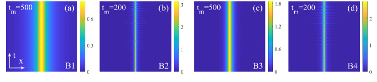
Figure 4: The perturbed evolution of the solitons corresponding to labels B1–B4 in Figs. 3(a,c). The respective values of the parameters are $\alpha=1.1$, $g=1$, $\mu=-0.2$ (a); $\alpha=1.1$, $\mu=-2$ (b); $\alpha=1.7$, $\mu=-1.5$ (c); $\alpha=1.1$, $\mu=-1.5$ (d). The evolution is plotted in the spatial domain $-10<x<+10$. Values $\mathrm{t}_{\mathrm{m}}$ indicate intervals of the scaled propagation distance in the respective panels, $0<z<\mathrm{t}_{\mathrm{m}}$. In panels (a) and (c), larger $\mathrm{t}_{\mathrm{m}}$ is taken to corroborate the full stability of the solitons. The plots are borrowed from Ref. [47] (unpublished).

III Further results for nonlinear modes in one-dimensional fractional waveguides

III.1 Systems with trapping potentials

While the possibility of the collapse in fractional NLSE (1) gives rise to instability of all solitons at $\alpha\leq 1$ in the free space (with $V=0$), the parabolic trapping potential,

$$V(x)=\left(\Omega^{2}/2\right)x^{2},$$ (32)

helps to create stable solitons even in this case [34]. This finding is similar to the well-known fact that the parabolic trap lifts the norm degeneracy of the Townes solitons and stabilizes their entire family against the critical collapse in the framework of the usual two-dimensional NLSE with the cubic self-attraction [54, 55]. Moreover, the same potential makes it possible to predict the existence of stable higher-order (multi-peak) solutions of Eq. (1). Such solutions may be considered as a nonlinear extension of various excited bound states maintained by the parabolic trapping potential in the linear Schrödinger equation. The latter finding is similar to the ability of the 2D parabolic potential to partly stabilize a family of trapped vortex solitons with winding number $n=1$ (i.e., the lowest-order excited states in 2D), in the framework of the cubic self-attractive NLSE [54, 55].

The higher-order solitons of orders $n=1,2,3,...$ , supported by Eq. (8) with potential (32), may be approximated by the commonly known stationary wave functions of eigenstates of the quantum-mechanical harmonic oscillator (corresponding to $\alpha=2$),

$$U(x)=A\exp\left(-\frac{\Omega}{2}x^{2}\right)H_{n}(x),$$ (33)

where $H_{n}(x)$ are Hermite polynomials, and $A$ is an amplitude. An example of a stable dipole-mode soliton, corresponding to $n=1$, and its fit provided by Eq. (33) with properly chosen $A$, is displayed in Fig. 5 for $\alpha=1$, which corresponds to the limit of the collapse-induced instability in the free space.

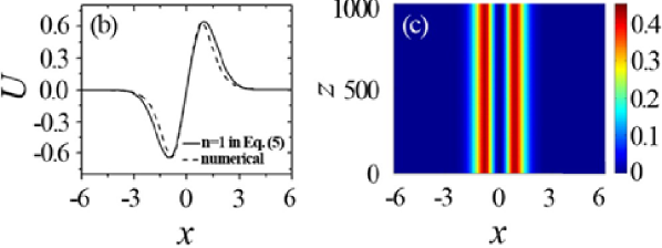
Figure 5: An example of a stable dipole-mode soliton produced by Eq. (1) with Lévy index $\alpha=1$, parabolic trapping potential (32) with $\Omega^{2}=1$, i.e., $V(x)=0.5x^{2}$, and nonlinearity strength $g=0.5$. The propagation constant of this state is $-\mu=1.16$. The stationary profile of the soliton and its propagation, in terms of the local-power distribution, are displayed in the left and right panels, respectively The solid line in the left panel represents the analytical fit provided by Eq. (33) with $n=1$. Reprinted with permission from Ref. [34]. Copyright 2020 Elsevier.

Another noteworthy effect induced by the potential term in the fractional NLSE was recently considered in Ref. [42], which addressed Eq. (1) with a double-well potential, viz.,

$$V(x)=-V_{0}\left[\exp\left(-\left(\frac{x+x_{0}}{w}\right)^{2}\right)+\exp\left(-\left(\frac{x-x_{0}}{w}\right)^{2}\right)\right],$$ (34)

with $V_{0}>0$ and width $w$. Equation (1) with this potential may support solitons which are symmetric or antisymmetric with respect to the two potential wells. An effect previously studied in detail in the framework of the usual NLSE (with $\alpha=2$) is that, when the soliton’s power exceeds a critical value, i.e., the nonlinearity is strong enough, symmetric solitons become unstable and are replaced by stable asymmetric ones, in the case of the self-focusing nonlinearity, i.e., $g>0$ in Eq. (1), while antisymmetric solitons remain stable with the increase of their norm [56]. Alternatively, an antisymmetry-breaking bifurcation takes place with antisymmetric solitons (while the symmetric ones remain stable) when the soliton’s norm exceeds a critical value in the case of the self-defocusing nonlinearity, corresponding to $g<0$ in Eq. (1). Such symmetry– and antisymmetry-breaking bifurcations (phase transitions) in the fractional NLSE with potential (34) are shown, severally, in Figs. 6 and 7 for the Lévy index $\alpha=1.1$, which makes the system essentially different from the usual NLSE, corresponding to $\alpha=2$.

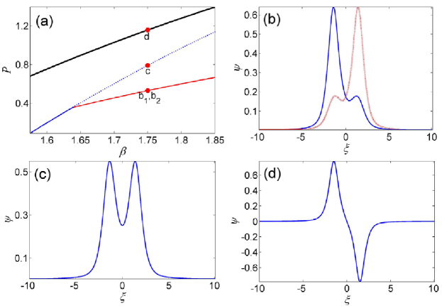
Figure 6: (a) Blue, red, and black lines show the norm (alias power, here denoted $P$) of symmetric, asymmetric, and antisymmetric solitons vs. their propagations constants (denoted $\beta\equiv-\mu$ here) in the fractional system based on Eq. (1) with $g=1$ (the self-focusing nonlinearity) and the double-well potential (34). The solid and dotted segments of the blue line represent, respectively, stable and unstable subfamilies of symmetric solitons, below and above the symmetry-breaking bifurcation. The branches of antisymmetric and asymmetric solitons are completely stable. Here and in Figs. 7 and 8 parameters of potential (34) are $V_{0}=1$, $w=1.4$, $x_{0}=1.5$. Panels (b), (c), and (d) display, severally, a pair of stable asymmetric solitons (mirror images of each other), an unstable symmetric soliton, and a stable antisymmetric one, all taken at $\beta=1.75$ (these solitons correspond to dots b_1,2, c, and d in panel (a)). Reprinted with permission from Ref. [42]. Copyright 2020 Elsevier.

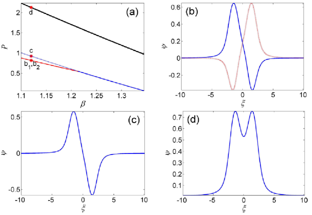
Figure 7: (a) Blue, red, and black lines show, respectively, the norm (power, here denoted $P$) of antisymmetric, asymmetric, and symmetric solitons vs. their propagations constants (denoted $\beta\equiv-\mu$ here) in the fractional system based on Eq. (1) with the double-well potential (34) and $g=-1$ (the self-defocusing nonlinearity). Other parameters are the same as in Fig. 6. The solid and dotted segments of the blue line represent, respectively, stable and unstable subfamilies of antisymmetric solitons, below and above the symmetry-breaking bifurcation. The branches of antisymmetric and asymmetric solitons are completely stable. Panels (b), (c), and (d) display, severally, a pair of stable asymmetric solitons (mirror images of each other), an unstable antisymmetric soliton, and a stable symmetric one, all taken at $\beta=1.12$ (these solitons correspond to dots b_1,2, c, and d in panel (a)). Reprinted with permission from Ref. [42]. Copyright 2020 Elsevier.

As shown in Fig. 8(a), simulations of the perturbed evolution, performed for the present model in Ref. [42], demonstrate that an unstable symmetric soliton (in the case of the self-attractive nonlinearity) breaks its symmetry and spontaneously transforms into a dynamical state which is close to either one of stable asymmetric solitons existing with the same power (a chiral pair of such solitons is shown in Fig. 6(b)). On the other hand, simulations of the evolution of unstable antisymmetric solitons (in the case of the self-repulsion) produce a different result, as shown in Fig. 8(b): the soliton does not tend to spontaneously transform into either one of the mutually chiral asymmetric solitons, but instead oscillates between them.

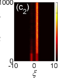
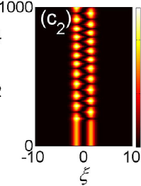
Figure 8: The perturbed evolution of unstable symmetric (a) and antisymmetric (b) solitons, produced by simulations of Eq. (1) with the double-well potential (34), Lévy index $\alpha=1.1$, and nonlinearity strength $g=+1$ (a) and $-1$ (b). The propagation constants of the unstable symmetric and antisymmetric solitons are $\mu=-1.62$ and $\mu=-1.12$, respectively. Reprinted with permission from Ref. [42]. Copyright 2020 Elsevier.

Furthermore, the action of the trapping potential (34), even if it is essentially weaker than the parabolic potential (32), provides an effect similar to the above-mentioned one induced by potential (32), viz., stabilization of symmetric, antisymmetric, and asymmetric solitons in the case of $\alpha\leq 1$, when all solitons are unstable in the free space, due of the occurrence of the critical ($\alpha=1$) or supercritical ($\alpha<1$) collapse. In particular, it was demonstrated that the symmetry-breaking bifurcation, quite similar to the one displayed in Fig. 6 (thus, including stable soliton branches) takes place in the same system at $\alpha=0.8$ [42].

III.2 Dissipative solitons produced by the fractional complex Ginzburg-Landau equation (CGLE)

An essential extension of the fractional NLSE was proposed in Ref. [39], in the form of the equation with complex coefficients (including the coefficient in front of the fractional-diffraction term), i.e., the fractional CGLE. It models the propagation of light in waveguides which, in addition to the fractional diffraction, include losses and gain:

$$i\frac{\partial\Psi}{\partial z}=-i\delta\Psi+\left(\frac{1}{2}-i\beta\right)\left(-\frac{\partial^{2}}{\partial x^{2}}\right)^{\alpha/2}\Psi+\left(i\varepsilon-1\right)\left|\Psi\right|^{2}\Psi+\left(-i\mu+\nu\right)|\Psi|^{4}\Psi,$$ (35)

where $\delta>0$, $\mu>0$, and $\beta\geq 0$ account for, respectively, the linear, quintic, and diffraction losses (fractional diffusion), $\varepsilon>0$ is the cubic gain, while $\nu\geq 0$ represents quintic self-defocusing, if it is present in the medium, and the cubic self-focusing term is the same as in Eq. (1) with $g=1$.

Equation (35) gives rise to dissipative solitons. Unlike those in the conservative NLSE, dissipative solitons exist not in families parametrized by the propagation constant, but as isolated localized solutions, whose stability is the major issue [39]. Systematic simulations of Eq. (35) have produced charts of different dynamical states, which are displayed in Fig. 9. The charts demonstrate a broad parameter region in which stable dissipative solitons appear.

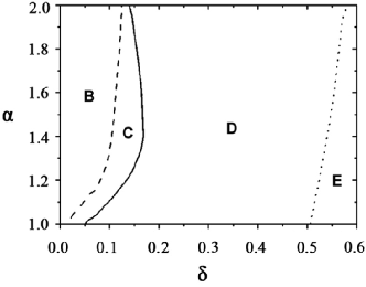
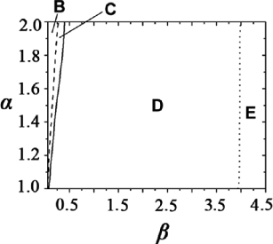
Figure 9: Charts of different established states produced by simulations of the fractional CGLE with the cubic-quintic nonlinearity (35), plotted in planes of the most essential parameters: linear loss $\delta$ and Lévy index $\alpha$ ((a), with fixed $\beta=0.1$), or the fractional-diffusion coefficient $\beta$ and $\alpha$ ((b), with $\delta=0.1$). Other coefficients are $\varepsilon=1.7$, $\mu=1$, and $\nu=0.115$. In the underdamped (low-loss) parameter area B, a uniform state extends, in direct simulations, to occupy the entire spatial domain. In areas C and D, stable dissipative solitons emerge (directly in D, and via an initial unstable-evolution stage in C). The input decays to zero in the overdamped area E. Reprinted with permission from Ref. [39]. Copyright 2020 Elsevier.

It is worthy to note that interaction between stable in-phase dissipative solitons, initially separated by some distance, leads to their merger into a single one, as shown in Fig. 10. It is seen that the merger is extremely slow in the case of the usual diffraction ($\alpha=2$), while the fractional diffraction essentially accelerates the process, due to the fact that the respective operator (2) actually makes the interaction between the separated solitons nonlocal, i.e., stronger.

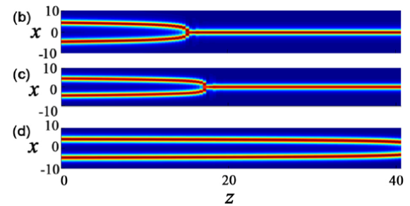
Figure 10: The merger of initially separated stable dissipative solitons, with zero phase difference between them, as produced by simulations of the fractional cubic-quintic CGLE (35), with parameters $\delta=0.3$, $\beta=0.1$, $\varepsilon=1.7$, $\nu=0.115$, $\mu=1$, and different values of the Lévy index: $\alpha=1.5$ (b), $1.8$ (c), and $2.0$ (d). Reprinted with permission from Ref. [39]. Copyright 2020 Elsevier.

IV Vortex modes in two-dimensional (2D) fractional-diffraction settings

IV.1 Stationary vortex solitons

As concerns the propagation of light beams with a 2D transverse structure in fractional media, the transmission of Airy waves, including ones carrying intrinsic vorticity (the optical angular momentum), was analyzed in the framework of the linear variant of Eq. (5) with $g=V=0$ [57, 58]. In particular, it is worthy to note that the tightest self-focusing of the Airy-ring input is attained at the value of the Lévy index $\alpha\approx 1.4$, which is essentially different from $\alpha=2$ corresponding to the normal 2D diffraction.

Dynamics of vortex solitons and vorticity-carrying ring-shaped soliton clusters was recently addressed in Refs. [31, 35], and [48] in the framework of the fractional NLSE with the cubic-quintic nonlinearity:

$$i\frac{\partial\Psi}{\partial z}=\frac{1}{2}\left(-\frac{\partial^{2}}{\partial x^{2}}-\frac{\partial^{2}}{\partial y^{2}}\right)^{\alpha/2}\Psi-\left|\Psi\right|^{2}\Psi+|\Psi|^{4}\Psi,$$ (36)

cf. Eq. (35). The 2D fractional-diffraction operator in Eq. (36) is defined as per Eq. (6).

Stationary solutions to Eq. (36), with propagation constant $-\mu>0$, integer vorticity (alias winding number) $s$, and real amplitude function $\Phi(r)$, are looked for, in polar coordinates $\left(r,\theta\right)$, as

$$\Psi=\exp\left(-i\mu z+is\theta\right)U(r).$$ (37)

Unlike the NLSE with the usual diffraction ($\alpha=2$), the substitution of ansatz (37) in Eq. (36) with the fractional diffraction operator is not trivial. Nevertheless, using the definition (6) of the operator, the respective calculation can be performed, demonstrating that the vortex ansatz is compatible with Eq. (36) (in other words, the angular-momentum operator commutes with the system’s Hamiltonian), the resulting equation being

$$\mu U=\frac{1}{2}\left(-\nabla_{r}^{2}\right)^{\alpha/2}U-U^{3}+U^{5},$$ (38)

where the fractional radial Laplacian is obtained in a cumbersome form:

$$\left(-\nabla_{r}^{2}\right)^{\alpha/2}U(r)=\frac{1}{2\pi}\int_{0}^{\infty}q^{\alpha+1}dq\int_{0}^{\infty}r^{\prime}dr^{\prime}\int_{0}^{2\pi}d\chi\cos\left(s\chi\right)J_{0}\left(q\sqrt{r^{2}+\left(r^{\prime}\right)^{2}-2rr^{\prime}\cos\chi}\right)U(r^{\prime}),$$ (39)

with Bessel function $J_{0}$.

Localized solutions of Eq. (38) are characterized by the 2D norm,

$$N_{\mathrm{2D}}\equiv\int\int\left|\Psi\left(x,y\right)\right|^{2}dxdy\equiv 2\pi\int_{0}^{\infty}U^{2}(r)rdr.$$ (40)

In the absence of the self-defocusing quintic term, a straightforward corollary of Eq. (38) with the cubic-only nonlinearity is a scaling relation between the norm and propagation constant, cf. Eq. (20):

$$N_{\mathrm{2D}}(\mu)=N_{0}(\alpha)\left(-\mu\right)^{1-2/\alpha}.$$ (41)

Obviously, at all values $\alpha\leq 2$ (i.e., at all relevant values of the Lévy index), this relation does not satisfy the VK criterion (21), that is why the inclusion of the quintic self-defocusing term is necessary for the stability of the resulting solitons, both fundamental ($s=0$) and vortical ones. Furthermore, due to the stabilizing effect of the quintic term, Eq. (36) supports stable localized states even in the case of $\alpha\leq 1$, when the cubic self-focusing alone gives rise to the collapse in the 1D setting. This stabilizing effect, which is maintained by the quintic nonlinearity in the free space, may be compared to the above-mentioned stabilization mechanism, provided by the trapping potential.

The distribution of the local power in soliton solutions with embedded vorticity (winding number) $s$ features a ring-like shape (see examples below in the left column of Fig. 13). Families of such solutions with $s=1,2,$ and $3$, produced by numerical solution of Eq. (38), are represented by dependences of the 2D norm on the propagation constant, which are displayed in Fig. 11. These dependences also highlight relatively small stable subfamilies of the vortex solitons. The stability was identified by the computation of eigenvalues, using linearized equations for small perturbations, and verified by direct simulations of the perturbed evolution [31].

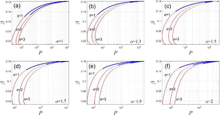
Figure 11: The propagation constant, $\beta\equiv-\mu$, vs. the norm (power) of the 2D solitons with vorticities $s=1,2$, and $3$. The power is defined here as $P\equiv 2^{2/\alpha}N_{\mathrm{2D}}$, see Eq. (40). The results are produced by the numerical solution of Eq. (38) for fixed values of the Lévy index: $\alpha=1$ (a), $1.3$ (b), $1.5$ (c), $1.7$ (d), $1.9$ (e), and $2$ (f). The latter case, corresponding to the usual two-dimensional NLSE, is included for comparison with the results produced by the fractional diffraction. Note that values of the power are shown on the logarithmic scale, which is different in different panels. Blue and red segments represent stable and unstable vortex states, respectively. Reprinted with permission from Ref. [31]. Copyright 2020 Elsevier.

In the limit of the diverging norm, the propagation constant in all panels of Fig. 11 attains the commonly known limit value for the NLSE with the cubic-quintic nonlinearity, $\beta_{\max}=3/16$ [59], which does not depend on the spatial dimension. Further, it is seen in the figure that the soliton families exist at values of the norm (power) exceeding a certain threshold value,

$$N\geq N_{\mathrm{thr}}^{(s)}(\alpha),$$ (42)

although the stability boundary corresponds to much larger values of the norm. Actually, this feature (i.e., the non-existence of solitons with the norm falling below a finite threshold value) is well known in models where the self-focusing nonlinear term, if acting alone, gives rise to the supercritical collapse, such as the three-dimensional NLSE with the normal diffraction [64]. Indeed, in collapse-free models solitons with a vanishingly small norm have a vanishing amplitude and diverging size, the latter fact implying $\mu\rightarrow-0$. However, Eq. (41) demonstrates that, at any $\alpha<2$, the norm of the solitons is diverging, rather than vanishing, at $\mu\rightarrow-0$, hence the limit of $N\rightarrow 0$ cannot be attained.

Dependences of the threshold norm on the Lévy index for $s=1,2,$ and $3$ are displayed in Fig. 12. In the limit of $\alpha=2$, i.e., in the case of the cubic-quintic NLSE with the normal 2D diffraction, the respective threshold values $N_{\mathrm{thr}}^{(s)}(\alpha=2)$ do not vanish either. They correspond to the Townes solitons of the 2D cubic NLSE with the embedded vorticity [65, 66, 7], cf. the norm given by Eq. (29) for the fundamental Townes solitons (with $s=0$):

$$N_{\mathrm{thr}}^{(s=1)}(\alpha=2)\approx 24.2;N_{\mathrm{thr}}^{(s=2)}(\alpha=2)\approx 44.9;N_{\mathrm{thr}}^{(s=3)}(\alpha=2)\approx 61.3.$$ (43)

As well as their fundamental counterparts, families of vortex Townes solitons are degenerate, in the sense that their norm takes the single value, which depends on $s$ but does not depend on the propagation constant. Actually, these values may be approximated by an analytical formula obtained in Ref. [67]: $N_{\mathrm{thr}}^{(s)}(\alpha=2)\approx 4\sqrt{3}\pi s$.

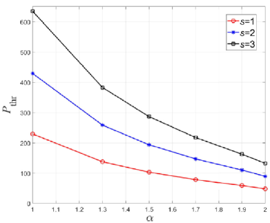
Figure 12: The threshold value of the power (norm), $P_{\mathrm{thr}}\equiv 2^{2/\alpha}N_{\mathrm{thr}}^{(s)}(\alpha)$, below which Eq. (38) cannot produce vortex solitons (see Eq. (42)), vs. the Lévy index $\alpha$, for vorticities $s=1,2,$ and $3$. In the limit of $\alpha=2$, which corresponds to the normal (non-fractional) diffraction, the threshold values $N_{\mathrm{thr}}^{(s)}(\alpha=2)$ coincide with the norms of the Townes solitons with the embedded vorticity, see Eq. (43). Reprinted with permission from Ref. [31]. Copyright 2020 Elsevier.

In simulations of Eq. (36) those vortex solitons which are unstable split in sets of separating fragments, as shown in Fig. 13. This is the usual instability-development scenario for vortex solitons in NLSEs with diverse nonlinearities [7].

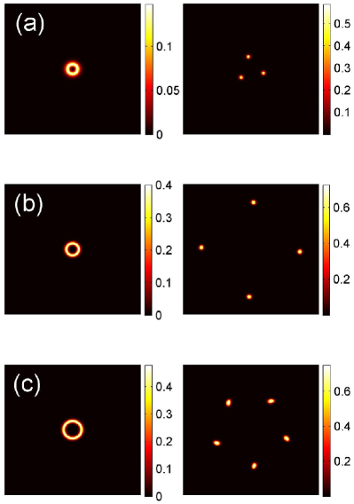
Figure 13: Spontaneous splitting of unstable ring-shaped vortex solitons, with winding numbers $s$ and propagation constants $\mu$, into sets of fragments, as produced by simulations of Eq. (40) with $\alpha=1.5$: (a) $\left(s,\mu=1,-0.03\right)$; (b) $\left(2,-0.08\right)$; (c) $\left(3,-0.095\right)$. The left and right panels display, respectively, the local power distribution in the input ($z=0$) and output, taken at $z=500$. All panels show the domain of the $(x,y)$ plane of the size $\left(-150,+1.150\right)\times\left(-150,+1.150\right)$. Reprinted with permission from Ref. [31]. Copyright 2020 Elsevier.

IV.2 Dynamics of vortical clusters

In addition to the axisymmetric stationary vortex solitons, it is relevant to consider the dynamics of necklace-shaped clusters. At $z=0$ they are composed as sets (circular chains) of $M$ fundamental solitons (with zero intrinsic winding numbers), with equal distances between them,

$$l=2R\sin\left(\pi/M\right),$$ (44)

and global vorticity, $S=1,2,3,...$, imprinted onto the cluster:

$$\Psi_{0}\left(x,y\right)=\exp\left(iS\theta\right)\sum_{m=1}^{M}U_{0}\left(\left|\mathbf{r}-\mathbf{r}_{m}\right|\right),$$ (45)

$$\mathbf{r}_{m}=R\left\{\cos\left(\frac{2\pi m}{M}\right),\sin\left(\frac{2\pi m}{M}\right)\right\}.$$ (46)

Here $U_{0}\left(\left|\mathbf{r}-\mathbf{r}_{m}\right|\right)$ is the stationary shape of the fundamental soliton with the center placed at point $\mathbf{r}=\mathbf{r}_{m}$, and $R$ is the radius of the cluster.

Previously, patterns of the necklace type have drawn much interest in studies of models based on NLSEs with normal diffraction [60, 61, 62]. In particular, robust soliton necklaces supported by the cubic-quintic nonlinearity (the same as in Eq. (36)) were addressed in Ref. [63].

The formation and stability of the circular soliton chains in the framework of Eq. (36) was studied in detail in Ref. [35]. Parameters of the input, taken in the form of Eqs. (45) and (46), were chosen so that the axisymmetric vortex soliton with the same vorticity $S$, and the norm equal to the total norm of the initial soliton chain, is stable, in terms of Fig. 11. A set of typical results produced by this input is displayed in Fig. 14. It is seen in row (a) of the figure that, in the absence of the overall vorticity ($S=0$), the input set of solitons promptly fuses into a stable fundamental soliton. On the other hand, if the vorticity is too large, $S\geq 2$, no bound state is formed, and the initial soliton chain quickly expands, as observed in Fig. 14(b).

The formation of quasi-stable slowly rotating necklaces is possible in the case of $S=1$. In Fig. 14(c), the necklace state features slow rotation in combination with periodic oscillations in the radial direction. On the other hand, Fig. 14(d) demonstrates an example of a rotating necklace with a nearly permanent shape, which remains stable in the course of very long propagation. Indeed, $z=1000$ in this case is tantamount, roughly, to $\sim 50$ diffraction (Rayleigh) lengths of the input pattern, which, in turn, may be estimated as $z_{\mathrm{Rayleigh}}\sim\left(2R\right)^{\alpha}$.

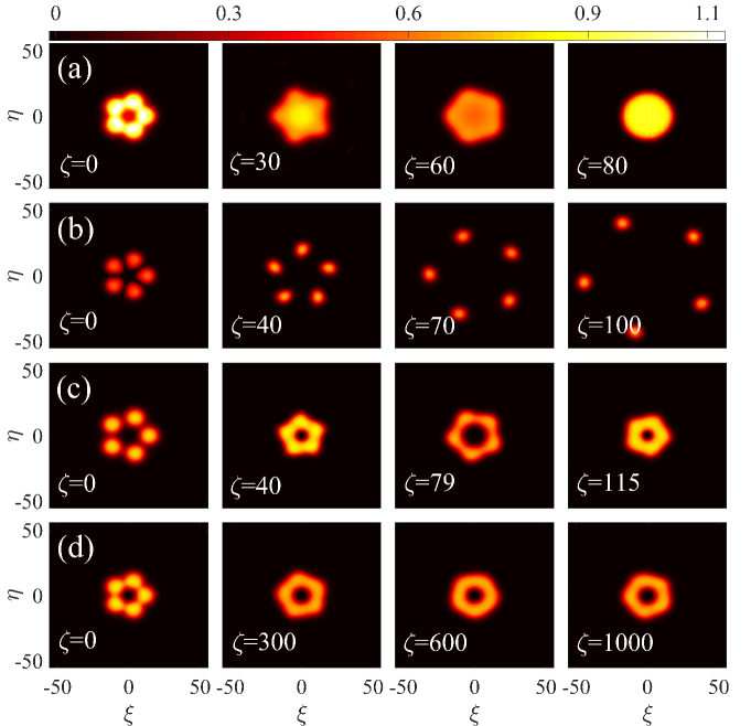
Figure 14: The evolution of necklace-shaped clusters initially built, as per Eqs. (45) and (44), of $M=5$ fundamental solitons, carrying overall vorticity $S=0$ (a), $S=2$ (b), and $S=1$ (c,d). The initial radii of the inputs, and the angular velocity of their rotation, produced by the evolution, are, respectively, $\left(R,\omega)=(11.25,0\right)$ (a); $\left(10.35,0.0128\right)$ (b); $\left(13,0.005\right)$ (c); and $\left(10.35,0.0071\right)$ (d). The results were produced by simulations of Eq. (36) with Lévy index $\alpha=1$. In this figure, coordinates $x$, $y$ and $z$ are denoted, respectively, as $\xi$, $\eta$ and $\zeta$. The figure is borrowed from Ref. [35].

IV.3 Stabilization of 2D solitons by the trapping potential

As said above, all soliton solutions of Eq. (5) with the cubic self-focusing nonlinearity ($g=1$) in the free space ($V=0$) are completely unstable at all values of the Lévy index, $\alpha\leq 2$. Instead of the quintic self-defocusing term, stabilization may be provided by the 2D parabolic potential,

$$V\left(x,y\right)=\left(\Omega^{2}/2\right)r^{2},$$ (47)

cf. Eq. (32). In an analytical form, this possibility can be demonstrated for small values of $\Omega^{2}$ in Eq. (47), competing with small fractality parameter $\left(2-\alpha\right)$, which determines the proximity to the normal diffraction ($\alpha=2$).

First, the effect of the weak trapping potential can be taken into regard by means of the respective VA for the NLSE including this potential, the regular diffraction ($\alpha=2$), and cubic self-focusing [68]. The VA for the stationary wave function with zero vorticity (see Eq. (37) with $s=0$) is based on the 2D Gaussian ansatz,

$$\mathcal{U}(r)=A\exp\left(-\frac{r^{2}}{2W^{2}}\right),$$ (48)

with the norm (see Eq. (40))

$$\mathcal{N}=\pi A^{2}W^{2},$$ (49)

cf. Eqs. (23) and (24). The respective expression for the effective Lagrangian is

$$L_{\mathrm{eff}}^{\mathrm{(2D)}}=-\frac{\mu}{2}\mathcal{N}+\frac{\mathcal{N}}{4W^{2}}-\frac{\mathcal{N}^{2}}{8\pi W^{2}}+\frac{\Omega^{2}}{4}\mathcal{N}W^{2},$$ (50)

cf. Eq. (25). The Euler-Lagrange equations following from here, $\partial L_{\mathrm{eff}}^{\mathrm{(2D)}}/\partial\left(W,\mathcal{N}\right)=0$, lead to an expression showing how potential (47) with small $\Omega^{2}$ lifts the norm degeneracy of the 2D Townes solitons:

$$\mathcal{N}\approx 2\pi\left(1-\frac{\Omega^{2}}{4\mu^{2}}\right).$$ (51)

Here, the first term corresponds to the above-mentioned VA prediction for the degenerate norm of the Townes solitons in the 2D cubic NLSE with the normal diffraction ($\alpha=2$), see Eq. (28). In the lowest approximation, a small effect of $\Omega^{2}$ may be neglected in the corresponding VA-predicted relation between the soliton’s width $W$ and propagation constant $-\mu$ :

$$W^{2}\approx-(2\mu)^{-1}.$$ (52)

While Eq. (51) pertains to $\alpha=2$, the expansion of the free-space ($V=0$) scaling relation (41) for small fractality, $0<2-\alpha\ll 1$, yields

$$N\approx 2\pi\left[1-\frac{2-\alpha}{2}\ln\left(-\mu\right)\right],$$ (53)

where the value of $N$ for the Townes soliton at $\alpha=2$ is substituted by the VA value (28). Combining Eqs. (51) and (53) yields an expression which makes it possible to analyze the competition of the stabilizing and destabilizing effects produced, respectively, by the trapping potential and the weak fractality:

$$N\approx 2\pi\left[1-\frac{\Omega^{2}}{4\mu^{2}}-\frac{2-\alpha}{2}\ln\left(-\mu\right)\right].$$ (54)

The stable part of the family of weakly-fractional solitons characterized by dependence (54) may be identified by means of the VK criterion (21). It predicts that stable solitons are those with the propagation constant $-\mu>0$ subject the following constraint:

$$\mu^{2}<\Omega^{2}/\left(2-\alpha\right).$$ (55)

Thus, according to Eq. (52), stable solitons should be wide enough, $W^{2}>\sqrt{2-\alpha}/\left(2\Omega\right)$. This conclusion is natural, as the soliton should be sufficiently wide to feel the stabilizing effect of the trapping potential.

V Conclusion

Studies of the wave propagation in fractional media have made remarkable progress, starting from the fractional linear Schrödinger equation, which was introduced by Laskin [9] for quantum-mechanical particles moving by Lévy flights. The fractality in that equation is represented by the derivative of the Riesz type, characterized by the Lévy index, $\alpha$. Actually, this is an integral operator (2), defined by means of the combination of direct and inverse Fourier transforms. This operator may be approximately reduced to a combination of usual local derivatives when it acts on the wave function built as a rapidly oscillating continuous-wave carrier multiplied by a slowly varying envelope, as shown by Eq. (13).

The next step was the realization of the fractional Schrödinger equation as one governing the paraxial wave propagation in optical setups emulating the fractional diffraction [13]. The implementation of the fractional Schrödinger equation in optics has made it natural to include the Kerr (as well as non-Kerr) nonlinearities, thus arriving at the fractional NLSE. The nonlinear equations render it possible to predict various self-trapped modes, such as solitons and solitary vortices, in these settings. The present article offers a brief review of some recent theoretical results on this topic, while experimental observations of fractional solitons have not been published, as yet. The modes considered in the review include basic 1D solitons and 2D solitary vortices in the free space, supported by the cubic and cubic-quintic nonlinearities, respectively. The 1D solitons are considered in the interval of values of the Lévy index $1<\alpha\leq 2$ (the fractional NLSE with the cubic self-focusing term in 1D gives rise to the collapse at $\alpha\leq 1$, while $\alpha=2$ corresponds to the usual diffraction term). All 2D solitons supported by cubic nonlinearity in the free space are unstable at $\alpha\leq 2$.

Also considered are 1D solitons in external potentials, which make it possible to produce stable higher-order (multiple-peak) solitons and study the spontaneous symmetry breaking in double-well potentials. In addition to that, trapping potentials may stabilize 1D solitons at $\alpha<1$ and 2D ones at $\alpha<2$. For the 2D setting, dynamics of necklace-shaped soliton clusters carrying overall vorticity is included too. Proceeding to the fractional cubic-quintic CGLE, the review briefly surveys 1D dissipative solitons predicted by that equation.

This mini-review is far from being a comprehensive one. Among other topics related to the fractional NLSEs are, inter alia, $\mathcal{PT}$-symmetric solitons maintained by complex potentials subject to condition (4). In particular, breaking and restoration of the solitons’ $\mathcal{PT}$ symmetry was recently considered in Ref. [16]. An interesting possibility is to introduce fractional equations of the NLSE type with quadratic or quadratic-cubic nonlinearity [69, 47]. Also theoretically considered were various modes supported by a modulationally stable background field (continuous wave), such as dark solitons and vortices, “bubbles”, and W-shaped solitons [51, 70].

The theory may be developed in other directions. In particular, NLSEs of a different type, that account for temporal propagation of optical waves under the action of the fractional group-velocity dispersion, were developed in Refs. [71] and [72]. The analysis has produced solitons in those models as well.

Conflicts of Interest

The author declares that there are no conflicts of interest related to this article.

References

- [1] Y. S. Kivshar, B. A. Malomed, Dynamics of solitons in nearly integrable systems, Rev. Mod. Phys. 61(4), 763-915 (1989).
- [2] B. A. Malomed, D. Mihalache, F. Wise, L. Torner, Spatiotemporal optical solitons. J. Opt. B 7, R53-R72 (2005).
- [3] Y. V. Kartashov, B.A. Malomed, L. Torner, Solitons in nonlinear lattices. Rev. Mod. Phys. 83, 247-306 (2011).
- [4] Z. Chen, M. Segev, D. N. Christodoulides, Optical spatial solitons: historical overview and recent advances. Rep. Prog. Phys. 75, 086401 (2012).
- [5] B. A. Malomed, Multidimensional solitons: Well-established results and novel findings. Eur. Phys. J. Spec. Top. 225, 2507-2532 (2016).
- [6] Y. V. Kartashov, G. E. Astrakharchik, B. A. Malomed, L. Torner, Frontiers in multidimensional self-trapping of nonlinear fields and matter. Nat. Rev. Phys. 1, 185-197 (2019).
- [7] B. A. Malomed, (INVITED) Vortex solitons: Old results and new perspectives, Physica D 399, 108-137 (2019).
- [8] D. Mihalache, Localized structures in optical and matter-wave media: A selection of recent studies, Rom. Rep. Phys. 73(2), 403 (2021).
- [9] N. Laskin, Fractional quantum mechanics and Lévy path integrals. Phys. Lett. A 268, 298-305 (2000).
- [10] N. Laskin, Fractional quantum mechanics (World Scientific: Singapore, 2018).
- [11] B. A. Stickler, Potential condensed-matter realization of space-fractional quantum mechanics: The one-dimensional Lévy crystal. Phys. Rev. E 88, 012120 (2013).
- [12] F. Pinsker, W. Bao, Y. Zhang, H. Ohadi, A. Dreismann, and J. J. Baumberg, Fractional quantum mechanics in polariton condensates with velocity-dependent mass. Phys. Rev. B 92, 195310 (2015).
- [13] S. Longhi, Fractional Schrödinger equation in optics. Opt. Lett. 40, 1117-1120 (2015).
- [14] Y. Zhang, X. Liu, M. R. Belić, W. Zhong, Y. Zhang, M. Xiao, Propagation dynamics of a light beam in a fractional Schrödinger equation, Phys. Rev. Lett. 115(18), 180403 (2015).
- [15] Y. Zhang, H. Zhong, M. R. Belić, Y. Zhu, W. Zhong, Y. Zhang, D. N. Christodoulides, M. Xiao, symmetry in a fractional Schrödinger equation, Laser Photonics Rev. 10(3), 526-531 (2016).
- [16] P. Li, B. A. Malomed and D. Mihalache, Symmetry-breaking bifurcations and ghost states in the fractional nonlinear Schrödinger equation with a -symmetric potential, Opt. Lett. 46, 3267-3270 (2021).
- [17] L. Zhang, Z. He, C. Conti, Z. Wang, Y. Hu, D. Lei, Y. Li, and D. Fan, Modulational instability in fractional nonlinear Schrödinger equation, Commun. Nonlin. Sci. Numer. Simulat. 48, 531-540 (2017).
- [18] S. Secchi and M. Squassina, Soliton dynamics for fractional Schrödinger equations, Applicable Analysis, 93, 1702-1729 (2014).
- [19] S. Duo and Y. Zhang, Mass-conservative Fourier spectral methods for solving the fractional nonlinear Schrödinger equation, Computers and Mathematics with Applications 71, 2257-2271 (2016).
- [20] W. P. Zhong, M. R. Belić, B. A. Malomed, Y. Zhang, and T. Huang, Spatiotemporal accessible solitons in fractional dimensions, Phys. Rev. E 94, 012216 (2016).
- [21] W. P. Zhong, M. R. Belić, and Y. Zhang, Accessible solitons of fractional dimension, Ann. Phys. 368, 110-116 (2016).
- [22] Y. Hong and Y. Sire, A new class of traveling solitons for cubic fractional nonlinear Schrödinger equations, Nonlinearity 30, 1262-1286 (2017).
- [23] M. Chen, S. Zeng, D. Lu, W. Hu, and Q. Guo, Optical solitons, self-focusing, and wave collapse in a space-fractional Schrödinger equation with a Kerr-type nonlinearity, Phys. Rev. E 98, 022211 (2018).
- [24] Q. Wang, J. Li, L. Zhang, and W. Xie, Hermite-Gaussian-like soliton in the nonlocal nonlinear fractional Schrödinger equation, EPL 122, 64001 (2018).
- [25] Q. Wang, and Z. Z. Deng, Elliptic Solitons in (1+2)-dimensional anisotropic nonlocal nonlinear fractional Schrödinger equation, IEEE Photonics J. 11, 1-8 (2019).
- [26] C. Huang and L. Dong, Gap solitons in the nonlinear fractional Schrödinger equation with an optical lattice, Opt. Lett. 41, 5636-5639 (2016).
- [27] J. Xiao, Z. Tian, C. Huang, and L. Dong, Surface gap solitons in a nonlinear fractional Schrödinger equation, Opt. Express 26, 2650-2658 (2018).
- [28] L. F. Zhang, X. Zhang, H. Z. Wu, C. X. Li, D. Pierangeli, Y. X. Gao, and D. Y. Fan, Anomalous interaction of Airy beams in the fractional nonlinear Schrödinger equation, Opt. Exp. 27, 27936-27945 (2019).
- [29] L. Dong and Z. Tian, Truncated-Bloch-wave solitons in nonlinear fractional periodic systems, Ann. Phys. 404, 57-64 (2019).
- [30] L. Zeng and J. Zeng, One-dimensional gap solitons in quintic and cubic-quintic fractional nonlinear Schrödinger equations with a periodically modulated linear potential, Nonlinear Dyn. 98, 985-995 (2019).
- [31] P. Li, B. A. Malomed, and D. Mihalache, Vortex solitons in fractional nonlinear Schrödinger equation with the cubic-quintic nonlinearity, Chaos Solitons Fract. 137, 109783 (2020).
- [32] Q. Wang and G. Liang, Vortex and cluster solitons in nonlocal nonlinear fractional Schrödinger equation, J. Optics 22, 055501 (2020)
- [33] L. Zeng and J. Zeng, One-dimensional solitons in fractional Schrödinger equation with a spatially periodical modulated nonlinearity: nonlinear lattice, Opt. Lett. 44, 2661-2664 (2019).
- [34] Y. Qiu, B. A. Malomed, D. Mihalache, X. Zhu, X. Peng, and Y. He, Stabilization of single- and multi-peak solitons in the fractional nonlinear Schrödinger equation with a trapping potential, Chaos Solitons Fract. 140, 110222 (2020).
- [35] P. Li, B. A. Malomed, and D. Mihalache, Metastable soliton necklaces supported by fractional diffraction and competing nonlinearities, Opt. Exp. 28, 34472-33488 (2020).
- [36] L. Zeng, D. Mihalache, B. A. Malomed, X. Lu, Y. Cai, Q. Zhu, and J. Li, Families of fundamental and multipole solitons in a cubic-quintic nonlinear lattice in fractional dimension, Chaos Solitons Fract. 144, 110589 (2021).
- [37] L. Zeng and J. Zeng, Preventing critical collapse of higher-order solitons by tailoring unconventional optical diffraction and nonlinearities, Commun. Phys. 3, 26 (2020).
- [38] M. I. Molina, The fractional discrete nonlinear Schrödinger equation, Phys. Lett. A 384, 126180 (2020)
- [39] Y. Qiu, B. A. Malomed, D. Mihalache, X. Zhu, L. Zhang, and Y. He, Soliton dynamics in a fractional complex Ginzburg-Landau model, Chaos Solitons Fract. 131, 109471 (2020).
- [40] P. Li, J. Li, B. Han, H. Ma, and D. Mihalache, D.: -symmetric optical modes and spontaneous symmetry breaking in the space-fractional Schrödinger equation, Rom. Rep. Phys. 71, 106 (2019).
- [41] Li, P., Dai C.: Double Loops and Pitchfork Symmetry Breaking Bifurcations of Optical Solitons in Nonlinear Fractional Schrödinger Equation with Competing Cubic-Quintic Nonlinearities, Ann. Phys. (Berlin) 532, 2000048 (2020).
- [42] P. Li, B. A. Malomed, and D. Mihalache, Symmetry breaking of spatial Kerr solitons in fractional dimension, Chaos Solitons Fract. 132, 109602 (2020).
- [43] L. Zeng, and J. Zeng, Fractional quantum couplers, Chaos Solitons Fract, 140, 110271 (2020).
- [44] L. Zeng, J. Shi, X. Lu, Y. Cai, Q. Zhu, H. Chen, H. Long, and J. Li, Stable and oscillating solitons of -symmetric couplers with gain and loss in fractional dimension. Nonlinear Dyn. 103, 1831-1840 (2021).
- [45] M. Cai and C. P. Li, On Riesz derivative, Fractional Calculus and applied analysis 22, 287-301 (2019).
- [46] D. S. Petrov and G. E. Astrakharchik, Ultradilute low-dimensional liquids, Phys. Rev. Lett. 117, 100401 (2016).
- [47] L. Zeng, Y. Zhu, B. A. Malomed, D. Mihalache, Q. Wang, H. Long, Y. Cai, X. Lu, and J. Li, Quadratic fractional solitons, to be published.
- [48] P. Li, R. Li, and C. Dai, Existence, symmetry breaking bifurcation and stability of two-dimensional optical solitons supported by fractional diffraction, Opt. Exp. 29, 3193-3210 (2021).
- [49] N. G. Vakhitov and A. A. Kolokolov, Stationary solutions of the wave equation in a medium with nonlinearity saturation. Radiophys. Quantum Electron. 16(7), 783-789 (1973).
- [50] L. Bergé, Wave collapse in physics: principles and applications to light and plasma waves, Phys. Rep. 303, 259-370 (1998).
- [51] L. Zeng, B. A. Malomed, D. Mihalache, Y. Cai, X. Lu, Q. Zhu, and J. Li, Bubbles and W-shaped solitons in Kerr media with fractional diffraction, Nonlinear Dynamics 104, 4253-4264 (2021).
- [52] S. I. Muslih, O. P. Agrawal, and D. Baleanu, A Fractional Schrödinger equation and its solution, Int. J. Theor. Phys. 49, 1746-1752 (2010).
- [53] M. Desaix, D. Anderson, and M. Lisak, Variational approach to collapse of optical pulses, J. Opt. Soc. Am. B 8, 2082-2086 (1991).
- [54] T. J. Alexander and L. Bergé, Ground states and vortices of matter-wave condensates and optical guided waves, Phys Rev E 65, 026611 (2001).
- [55] D. Mihalache, D. Mazilu, B. A. Malomed and F. Lederer, Vortex stability in nearly two-dimensional Bose-Einstein condensates with attraction, Phys Rev. A 73, 043615 (2006).
- [56] B. A. Malomed, editor: Spontaneous Symmetry Breaking, Self-Trapping, and Josephson Oscillations, (Springer-Verlag: Berlin and Heidelberg, 2013).
- [57] S. He, B. A. Malomed, D. Mihalache, X. Peng, X, Yu, Y. He, and D. Den, Propagation dynamics of abruptly autofocusing circular Airy Gaussian vortex beams in the fractional Schrödinger equation, Chaos, Solitons & Fractals 142, 110470 (2021).
- [58] S. He, B. A. Malomed, D. Mihalache, X. Peng, Y. He, and D. Deng, Propagation dynamics of radially polarized symmetric Airy beams in the fractional Schrödinger equation, Phys. Lett. A 404, 127403 (2021).
- [59] Kh. I. Pushkarov, D. I. Pushkarov, and I. V. Tomov, Self-action of light beams in nonlinear media: soliton solutions, Opt. Quant. Electr. 11, 471-478 (1979).
- [60] M. Soljačić and M. Segev, Integer and fractional angular momentum borne on self-trapped necklace-ring beams, Phys. Rev. Lett. 86, 420-423 (2001).
- [61] A. S. Desyatnikov and Y. S. Kivshar, Necklace-ring vector solitons, Phys. Rev. Lett. 87, 033901 (2001).
- [62] Y. V. Kartashov, L.-C. Crasovan, D. Mihalache, and L. Torner, Robust propagation of two-color soliton clusters supported by competing nonlinearities, Phys. Rev. Lett. 89, 273902 (2002).
- [63] D. Mihalache, D. Mazilu, L.-C. Crasovan, B. A. Malomed, F. Lederer, and L. Torner, Robust soliton clusters in media with competing cubic and quintic nonlinearities, Phys. Rev. E 68, 046612 (2003).
- [64] D. Mihalache, D. Mazilu, L.-C. Crasovan, I. Towers, A. V. Buryak, B. A. Malomed, L. Torner, J. P. Torres, and F. Lederer, Stable spinning optical solitons in three dimensions, Phys. Rev. Lett. 88, 073902 (2002).
- [65] V. I. Kruglov and R. A. Vlasov, Spiral self-trapping propagation of optical beams, Phys. Lett. A 111, 401-404 (1985).
- [66] V. I. Kruglov, Yu. A. Logvin, and V. M. Volkov, The theory of spiral laser beams in nonlinear media, J. Modern Opt. 39, 2277-2291 (1992).
- [67] J. Qin, G. Dong, and B. A. Malomed, Stable giant vortex annuli in microwave-coupled atomic condensates, Phys. Rev. A 94, 053611 (2016).
- [68] Z. Chen, Y. Li, B. A. Malomed, and L. Salasnich, Spontaneous symmetry breaking of fundamental states, vortices, and dipoles in two and one-dimensional linearly coupled traps with cubic self-attraction, Phys. Rev. A 96, 033621 (2016).
- [69] J. Thirouin, On the growth of Sobolev norms of solutions of the fractional defocusing NLS equation on the circle, Ann. Inst. H. Poincare AN34, 509-531 (2017).
- [70] L. Zeng, B. A. Malomed, D, Mihalache, Y. Cai, X. Lu, Q. Zhu, and J. Li, Flat-floor bubbles, dark solitons, and vortices stabilized by inhomogeneous nonlinear media, Nonlnear Dyn. 104, 4253-4264 (2021).
- [71] J. Fujioka, A. Espinosa, and R. F. Rodríguez, Fractional optical solitons, Phys. Lett. A 374, 1126-1134 (2010).
- [72] J. Fujioka, A. Espinosa, R. F. Rodríguez, and B. A. Malomed, Radiating subdispersive fractional optical solitons, Chaos 24, 033121 (2014).