Star-Struck by Fixed Embeddings:
Modern Crossing Number Heuristics

Abstract

We present a thorough experimental evaluation of several crossing minimization heuristics that are based on the construction and iterative improvement of a planarization, i.e., a planar representation of a graph with crossings replaced by dummy vertices. The evaluated heuristics include variations and combinations of the well-known planarization method, the recently implemented star reinsertion method, and a new approach proposed herein: the mixed insertion method. Our experiments reveal the importance of several implementation details such as the detection of non-simple crossings (i.e., crossings between adjacent edges or multiple crossings between the same two edges). The most notable finding, however, is that the insertion of stars in a fixed embedding setting is not only significantly faster than the insertion of edges in a variable embedding setting, but also leads to solutions of higher quality.

1 Introduction

Given a graph $G$, the crossing number problem asks for the minimum number of edge crossings in any drawing of $G$, denoted by $\mathit{cr}(G)$. This problem is NP-complete [19], even when $G$ is restricted to cubic graphs [23] or graphs that become planar after removing a single edge [7]. While the currently known integer linear programming approaches to the problem [16, 6, 15] solve sparse instances within a reasonable time frame [12], dense instances require the use of heuristics.

One such heuristic is the well-known planarization method [1, 21], which constructs a planarization, i.e., a planar representation of $G$ with crossings replaced by dummy vertices of degree $4$. The heuristic first computes a spanning planar subgraph of $G$ and then iteratively inserts the remaining edges. Several variants of the planarization method have been thoroughly evaluated, including different edge insertion algorithms and postprocessing strategies; see [10] for the latest study. In a recent paper [17], Clancy et al. present an alternative heuristic—the star reinsertion method—, which differs in two key aspects from the planarization method: It (i) starts with a full planarization (instead of a planar subgraph) that is iteratively improved by reinserting elements, and (ii) the reinserted elements are stars (vertices with their incident edges) rather than individual edges. These star insertions are performed using a straight-forward but never tried algorithm from literature [13]. Clancy et al. were faced with the problem that the implementations of the aforementioned heuristics were written in different languages, leading to incomparable running times. In their evaluation, they thus focus on variants of the star reinsertion method; their comparison with the planarization method only gives averages over (a quite limited number of) full instance sets and relies on old data from previous experiments.

Herein, we present a comprehensive experimental evaluation of a wide array of crossing minimization heuristics based on edge and star insertion encompassing all known strong candidates. This includes not only variants of the planarization and star reinsertion methods but also combined approaches. In addition, we present and evaluate a new heuristic that builds up a planarization from a planar subgraph using both star and edge insertions. All of these algorithms are implemented as part of the same framework, enabling us to accurately compare their running times. Furthermore, we suggest ways of simplifying the implementation of the heuristics, increasing their speed in practice, and improving their results—e.g., by properly handling crossings between adjacent edges and multiple crossings between the same two edges.

2 Preliminaries

In the following, we consider a connected undirected graph $G$ (that is usually simple, i.e., does not contain parallel edges or self-loops) with $n$ vertices and $m$ edges, denoted by $V(G)$ and $E(G)$ respectively. Let $\Delta$ be the maximum degree of any vertex in $V(G)$ and $N(v)\coloneqq\{w\mid({v},{w})\in E\}$ the neighborhood of a vertex $v$. Then, $v$ along with a subset of its incident edges $F\subseteq\{({v},{w})\in E\}$ is collectively called a star, denoted by $(v,F)$. Furthermore, a (combinatorial) embedding of a planar graph $G$ corresponds to a cyclic ordering of the edges around each vertex in $V(G)$ such that the resulting drawing can be realized without any edge crossings. This induces a set of cycles that bound the faces of the embedding. Based on a combinatorial embedding of the primal graph $G$, we can define the dual graph ${G}^{*}$, whose vertices correspond to the faces of $G$, and vice versa. For each primal edge $e\in E(G)$, there exists a dual edge ${e}^{*}\in E({G}^{*})$ between the dual vertices corresponding to the $e$-incident primal faces. Note that ${G}^{*}$ may be a multi-graph with self-loops even if $G$ is simple.

For the purpose of this paper, it is of particular concern how to insert an edge $({v_{1}},{v_{2}})$ into a planarization. First, it is necessary to find a corresponding insertion path, i.e., a sequence of faces $f_{1},\dots,f_{k}$ such that $v_{1}$ is incident to $f_{1}$, $v_{2}$ incident to $f_{k}$, and $f_{i}$ adjacent to $f_{i+1}$ for $i\in\{1,\dots,k-1\}$. An edge between $v_{1}$ and $v_{2}$ can then be inserted into a planarization by subdividing a common edge for each face pair $(f_{i},f_{i+1})$ and routing the new edge as a sequence of edges from $v_{1}$ along the subdivision vertices to $v_{2}$. By extension, the insertion spider of a star $(v,F)$ is a set of insertion paths, one for each edge in $F$. These insertion paths necessarily share a common face into which $v$ can be inserted.

3 Algorithms

3.1 Solving Insertion Problems

Insertion problems, and their efficient solutions, form the cornerstone of all known strong crossing minimization heuristics.

Definition 1 (EIF, SIF)

Given a planar graph $G$, an embedding $\Pi$ of $G$, and an edge (or star) not yet in $G$, insert this edge (star) into $\Pi$ such that the number of crossings in $\Pi$ is minimized. We refer to these problems as the edge (star) insertion problem with fixed embedding EIF (SIF, resp.).

Given a primal vertex $v$, let $\hat{v}$ be the vertex that is created by contracting the dual vertices that correspond to $v$-incident faces. Then, the EIF for any given edge $({v_{1}},{v_{2}})$ can be solved optimally in $\mathcal{O}(n)$ time by computing the shortest path from $\hat{v_{1}}$ to $\hat{v_{2}}$ in the dual graph ${G}^{*}$ via breadth-first search (BFS) [1]. By extension, the SIF for a star $(v,F)$ can be solved in $\mathcal{O}(|F|\cdot n)$ time as follows [13]: For each edge $(v,w)\in F$, solve the single-source shortest path problem in ${G}^{*}$ with $\hat{w}$ as the source (via BFS). For each face $f$, the sum over all of the resulting distance values at this $f$ then represents the number of crossings that would be created if $v$ was to be inserted into $f$. Hence, the face with the minimum distance sum is the optimal face to insert $v$ into, and the computed shortest paths to this face collectively form the insertion spider. To avoid crossings between these shortest paths (due to them not being necessarily unique), we can construct the insertion spider using a final BFS starting at the optimal face.

Definition 2 (EIV, MEIV, SIV)

Given a planar graph $G$ and an edge (a set of $k$ edges, or a star) not yet in $G$, find an embedding $\Pi$ among all possible embeddings of $G$ such that optimally inserting the edge (set of $k$ edges, star) into this $\Pi$ results in the minimum number of crossings. We refer to these problems as the edge (multiple edge, star) insertion problem with variable embedding EIV (MEIV, SIV, resp.).

The EIV can be solved in $\mathcal{O}(n)$ time using an algorithm by Gutwenger et al. [22], which finds a suitable embedding (with the help of SPR-trees) and then executes the EIF-algorithm described above. Now consider the MEIV: Solving it for general $k$ is NP-hard [27], however there exists an $\mathcal{O}(kn+k^{2})$-time approximation algorithm with an additive guarantee of $\Delta k\log k+\binom{k}{2}$ [14] that performs well in practice [10]. Put briefly, the EIV-algorithm is run for each of the $k$ edges independently, and a single final embedding is identified by combining the individual (potentially conflicting) solutions via voting. Then, the EIF-algorithm can be executed once for each edge. Note that the SIV can be solved optimally in polynomial time by using dynamic programming techniques [13]. However, for graphs that are not series-parallel, the resulting running times are exorbitant and there is no known implementation of this algorithm. In fact, our results herein suggest that in the context of crossing minimization heuristics, the solution power of the SIV-algorithm is fortunately not necessary in practice.

Each problem discussed above has a weighted version which can be solved in the same manner if each $c_{e}$-weighted edge $e$ is replaced by $c_{e}$ parallel $1$-weighted edges beforehand. In practice it is worthwhile to compute the shortest paths during the EIF/SIV-algorithm on the weighted instance directly. However, this does not allow for the same theoretical upper bounds of the running times since the weights may be arbitrarily large.

3.2 Crossing Minimization Heuristics

We start with reviewing several crossing minimization heuristics that iteratively build up a planarization, starting with a planar subgraph:

The planarization method (plm)

is the longest studied and best-known approach considered, achieving strong results in previous evaluations [1, 10, 21]. First, we compute a spanning planar subgraph $G^{\prime}=(V,E^{\prime})\subseteq G$, usually by employing a maximum planar subgraph heuristic and extending the result such that it becomes (inclusion-wise) maximal. Then, the remaining edges $F\coloneqq E\setminus E^{\prime}$ are either inserted one after another—by solving the respective EIF (fix) or EIV (var)—or simultaneously using the MEIV-approximation algorithm (multi). Gutwenger and Mutzel [21] describe a postprocessing strategy for plm based on edge insertion: Each edge is deleted from the planarization and reinserted one after another (all). To incrementally improve the planarization, all can also be executed once after each individual edge insertion (inc) [10]. In the following, we represent the use of these postprocessing strategies by appending the respective shorthand to the algorithm’s abbreviation, e.g. fix-all. When neither all nor inc is employed, we use the specifier none instead.

The chordless cycle method (ccm)

realizes the idea of extending a vertex-induced planar subgraph to a full planarization via star insertion [13]. It corresponds to the best-performing scheme for the star insertion algorithm as examined by Clancy et al. [17]: Search for a chordless cycle in $G$, e.g., via breadth-first search. Let $G^{\prime}$ denote the subgraph of $G$ that is already embedded and initialize it with this chordless cycle. Iteratively (until the whole graph is embedded) select a vertex $v\not\in V(G^{\prime})$ such that there exists at least one edge $({v},{w})$ that connects $v$ with the already embedded subgraph $G^{\prime}$; insert $v$ into $G^{\prime}$ by solving the SIF for the star $(v,~{}\{({v},{w})\in E\mid w\in V(G^{\prime})\})$.

The mixed insertion method (mim)

is a novel approach that we propose as an alternative to the planarization schemes above. It proceeds in a fashion that is similar to plm but relies on star insertion instead of edge insertion in as many cases as possible. Accordingly, let $G^{\prime}$ denote the subgraph of $G$ that is already embedded and initialize it with a spanning planar subgraph $(V,E^{\prime})\subseteq G$. Then, (attempt to) insert the remaining edges $F\coloneqq E\setminus E^{\prime}$ by reinserting at least one endpoint of each edge $e\in F$ via star insertion. Since removing and then reinserting a cut vertex of the planar subgraph $G^{\prime}$ would temporarily disconnect it, the cut vertices of the planar subgraph are computed (cf. [24]) and each edge $e\in F$ is processed as follows: If both endpoints of $e$ are cut vertices of $G^{\prime}$, insert the edge via edge insertion (we choose to do so in a variable embedding setting as such edge insertions happen rarely). If only one endpoint of the edge is a cut vertex, reinsert the other one. If neither endpoint of the edge is a cut vertex, the endpoint to be reinserted can be chosen freely—globally, this corresponds to finding a vertex cover on the graph induced by $F$ that has to include all vertices neighboring a cut vertex in $G^{\prime}$. Finding an optimal vertex cover is NP-hard [25]; therefore we compare several heuristics: For each edge $e$, choose one of the endpoints randomly (random), choose the one with the higher or lower degree in $G$ (high_G, low_G), choose the one with the higher or lower degree in the graph induced by all edges in $F$ not incident to a cut vertex in $G^{\prime}$ (high_F, low_F), or choose both endpoints (both). Each of the chosen vertices is then deleted from the planar subgraph and reinserted together with all of its edges in the original graph by solving the corresponding SIF.

Herein, we evaluate the aforementioned heuristics not only on their own but also in combination with the star reinsertion method (srm) by Clancy et al. [17], a postprocessing strategy based on star insertion. It starts with an already existing planarization, which may be constructed using any of the methods outlined above (or even more trivial ones, such as extracting a planarization from a circular layout of the vertices, which, however, is known to perform worse [17]). To represent that the result of an algorithm is improved via srm, we append “srm” to its abbreviation, e.g. fix-none-srm. The given planarization is thereby processed as follows: Iteratively choose a vertex $v$, delete $v$ from $G$, and reinsert it again by solving the SIF for the star $(v,v\times N(v))$. Continue the loop until there is no more vertex whose reinsertion improves the solution (in which case the latter is said to be locally optimal). Clancy et al. propose different methods for choosing $v$; here, we consider the scheme they report to be the best compromise between solution quality and running time: In each iteration, try to reinsert every vertex once and continue with the next iteration as soon as a vertex is found whose reinsertion improves the number of crossings in the planarization.

The original algorithm only updates a planarization once an actual improvement is found and resets it to its original state otherwise. We propose to never reset it. This approach is permissible as the SIF is solved optimally and the number of crossings hence never increases after the reinsertion of a star. Not resetting the planarization has the potential to save time in practice as it allows for a simpler implementation without any need to copy the dual graph.

4 A Note on Non-simple Crossings

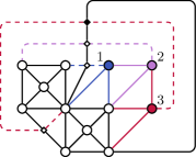
(a) Creation of an $\alpha$-crossing

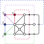
(b) Creation of a $\beta$-crossing

Figure 1: A non-simple crossing on the red dashed edge as the result of incrementally solving the same kind of insertion problem. When starting with the black planar subgraph, this may happen by solving the SIV using the described algorithm for the colored vertices in the order of their label numbers. Alternatively, if all solid edges constitute the initial planar subgraph, solving the EIV for the dashed edges in the order of their label numbers can have the same result. The examples apply both in the fixed and the variable embedding setting. Dummy vertices for (non-simple) crossings are represented by small (black) diamonds.

(a) Removal of an $\alpha$-crossing

(b) Removal of a $\beta$-crossing

Figure 2: Non-simple crossings between the red and green edges. After their removal (new edge paths drawn as dashed), the red edge is involved in a new non-simple crossing of the same type and the green edge in a new non-simple crossing of the opposite type. Thus, the removal procedure may have to be iterated.

It is well-known that any crossing-optimal drawing can be assumed to be simple: No edge self-intersects and each pair of edges intersects at most once (either in a crossing or an endpoint). In particular, a simple drawing may not contain crossings between adjacent edges ($\alpha$-crossings) or multiple crossings between the same two edges ($\beta$-crossings). We may hence call any such undesired crossings non-simple. Surprisingly, earlier implementations of the planarization method did not consider the emergence and removal of any non-simple crossings [10] while the implementation of the star reinsertion method by Clancy et al. only considers $\beta$- but not $\alpha$-crossings [17]. However, we show in Figure 1 that incrementally solving the same kind of insertion problem may result in a planarization with $\alpha$- or $\beta$-crossings, even when starting with a planar subgraph. Non-simple crossings can be removed by reassigning edges in the planarization to different edges in the original graph and then deleting the respective dummy vertices (see Figure 2). Doing so leads to better results overall, as shown in Appendix 0.C.

5 Experiments

Setup:

All algorithms are implemented in C++ as part of the Open Graph Drawing Framework (OGDF, www.ogdf.net, based on the release “2020.02 Catalpa”) [11], and compiled with GCC 8.3.0. Each computation is performed on a single physical processor of a Xeon Gold 6134 CPU (3.2 GHz), with a memory limit of 4 GB but no time limit. All instances and results are available for download at http://tcs.uos.de/research/cr.

Instances:

Table 1 lists the instance sets used for our evaluation (see Appendix 0.A for further statistical analysis). To enable a proper comparison of the tested algorithms (and potentially in the future, their competitors), we consider multiple well-known benchmark sets as well as constructed, random, and real-world instances with varying characteristics. These are preprocessed by computing the non-planar core (NPC) [9] for each non-planar biconnected component. We consider only those instances that have at least $25$ vertices after the NPC reduction unless the instance is part of the Complete, Complete-Bip., or KnownCR instance sets. Moreover, we precompute a planar subgraph and chordless cycle for each instance such that different runs of plm, mim and ccm can be started with the same initialization. The planar subgraph is computed by using Chalermsook and Schmid’s diamond algorithm [8] and extending the result to a maximal planar subgraph. On average, this computation took only 0.77% of the time needed to execute the fastest evaluated heuristic fix-none—a comparatively negligible amount of time that is not further taken into consideration during the evaluation.

Table 1: Considered instance sets. “#” denotes the number of graphs and $|V(G)|$ the (range of the) numbers of nodes—both values refer to the instance sets after preprocessing. Further, let $\delta$ denote the node degree, $\mathbin{\text{\scalebox{0.84}{$\square$}}}$ the Cartesian product of two graphs, $C_{i}$ the cycle with $i$ edges, $P_{j}$ the path with $j$ edges, and $G_{k}$ the $21$ non-isomorphic connected graphs on $5$ vertices indexed by $k$.

Name	#	$|V(G)|$	Description
Rome	3668	25–58	Well-known benchmark set [3], sparse
North	106	25–64	Well-known benchmark set collected by S. North [2]
Webcompute	75	25–112	Instances sent to our online tool [16] for the exact computation of crossing numbers, crossings.uos.de
Expanders	240	30–100	20 random regular graphs [26] (expander graphs with high probability) for each parameterization $(|V(G)|,\delta)\in\{30,50,100\}\times\{4,6,10,20\}$
Circuit-Based	45	26–3045	Hypergraphs from real world electrical networks, transformed into traditional graphs by replacing each hyperedge $h$ by a new hypervertex connected to all vertices contained in $h$
ISCAS-85 [5]	9	180–3045
ISCAS-89 [4]	24	60–584
ITC-99 [18]	12	26–980
KnownCR	1946	9–250	Benchmark set with $\mathit{cr}$ known through proofs [20]:
$C\mathbin{\text{\scalebox{0.84}{$\square$}}}C$	251	9–250	$\to$ $C_{i}\mathbin{\text{\scalebox{0.84}{$\square$}}}C_{j}$ with $3\leq i\leq 7$, $j\geq i$ such that $i\cdot j\leq 250$
$G\mathbin{\text{\scalebox{0.84}{$\square$}}}P$	893	15–245	$\to$ Subset of $G_{i}\mathbin{\text{\scalebox{0.84}{$\square$}}}P_{j}$ with $1\leq i\leq 21$, $3\leq j\leq 49$
$G\mathbin{\text{\scalebox{0.84}{$\square$}}}C$	624	15–250	$\to$ Subset of $G_{i}\mathbin{\text{\scalebox{0.84}{$\square$}}}C_{j}$ with $1\leq i\leq 21$, $3\leq j\leq 50$
$P(\_,\_)$	178	10–250	$\to$ Generalized Petersen graphs $P(2k+1,2)$ with $2\leq k\leq 62$ and $P(m,3)$ with $9\leq m\leq 125$
Complete	46	5–50	Complete graphs $K_{n}$ for $5\leq n\leq 50$
Complete-Bip.	666	10–80	Complete bipartite graphs $K_{n_{1},n_{2}}$ for $5\leq n_{1},n_{2}\leq 40$

The precomputed chordless cycle almost always consists of 3–6 vertices, containing 7–11 vertices for only 15 instances overall. How many edges are deleted to create the planar subgraph, on the other hand, varies greatly depending on the size and density of the graph. Of particular interest is the number of deleted edges that are incident to one or two cut vertices of the planar subgraph: During mim, the former ones have a fixed endpoint that must be reinserted via star insertion (disallowing a choice of the reinserted endpoint) while the latter ones must be inserted via edge insertion. Clearly, more dense instances such as the complete (bipartite) ones and the expanders require more edges to be deleted to form a planar subgraph. At the same time, due to their high connectivity, these instances also have less deleted edges that are connected to cut vertices in the planar subgraph. In particular, the complete (bipartite) instances do not have a single such edge. However, even on the sparser instances, mim inserts almost all edges via star insertion and one can usually choose the endpoint to be reinserted (see the mim-variants described in Subsection 3.2).

5.1 Fast Heuristics: Mixed Insertion Method, Chordless Cycle Method and Fixed Embedding Edge Insertion

The mim-variants, ccm, and fix-none (all without srm-postprocessing) are very fast but yield a comparably high number of crossings. Figure 3 displays some representative results on the expanders, contrasting them with the BEST solution found by 50 random permutations of any heuristic tested herein (cf. Subsection 5.4). Among the mim-variants, there are only little differences in computation speed and resulting number of crossings. However, reinserting both endpoints whenever a choice between two endpoints can be made clearly provides the best results across all instances while only taking an insignificant amount of additional time. The variant leads to the highest amount of reinserted stars and hence also to more chances for an improvement of the number of crossings. In contrast, high_F needs the lowest amount of star insertions and is thus the fastest variant (but provides results of mixed quality).

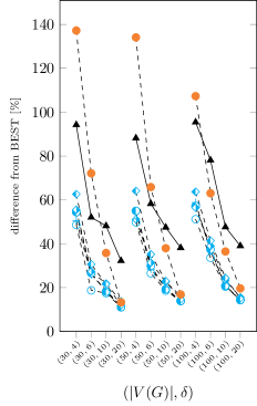
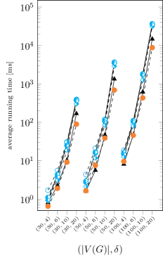
Figure 3: Comparison of the mim-variants, ccm and fix-none on the expanders.

Compared with fix-none and ccm, mim (from now on always referring to the both-variant) provides better results on almost all instances. The fastest of the algorithms, on the other hand, is fix-none. The last of the three, ccm, should only be considered when examining particularly dense instances: On sparse instance sets such as Rome or KnownCR, it is slower and yields far worse results than fix-none (which in turn yields worse results than mim), but the solution and speed disparity between the algorithms becomes smaller on instances with a higher density—see, e.g., Figure 3. On complete (bipartite) instances, ccm even surpasses mim both in terms of solution quality and speed.

5.2 Planarization Method

The different edge insertion algorithms and postprocessing strategies for the planarization method allow to greatly improve the final planarizations at the cost of additional running time. A detailed experimental comparison of these plm-variants was already carried out in 2012 [10]. We are able to replicate the results of that study and corroborate its claims with findings on additional instances:

In terms of solution quality, none provides much worse results than all and inc across all instance sets. However, postprocessing and inc in particular has the drawback of very high running times and a large amount of required memory. Among the edge insertion algorithms, var performs better (but is also slower) than multi, which in turn performs better than fix. Overall, fix-all is the fastest plm-variant that still benefits from the quality improvements of postprocessing. The best compromise between solution quality and speed is provided by the multi-variants while the best results are achieved by var-inc (cf. Appendix 0.B).

5.3 Improvements via the Star Reinsertion Method

We tested srm as a postprocessing method for the eight most promising and interesting algorithms that construct an initial planarization: The three fast algorithms mim, ccm, and fix-none, as well as the more involved fix-all, multi-all, multi-inc, var-all, and var-inc. In the case of the latter five, a form of postprocessing is already used, and the additional application of srm only leads to a small increase in running time, comparatively speaking. In the case of the former three, the additional postprocessing via srm significantly increases the running times (fix-none-srm becomes even slower than fix-all-srm), but the algorithms are still surprisingly fast: On sparse instances, the running times are comparable to multi-inc (without srm); on dense instances, the algorithms are even faster than fix-all. This is especially interesting as all srm-enhanced algorithms typically outperform even the best previously known heuristic variant var-inc (see Figures 4 and 5). In spite of its simplicity, star insertion in a fixed embedding setting is able to greatly improve intermediate planarizations by inserting multiple edges at once. It provides better results and is faster than edge insertion in a variable embedding setting even if the latter uses incremental postprocessing.

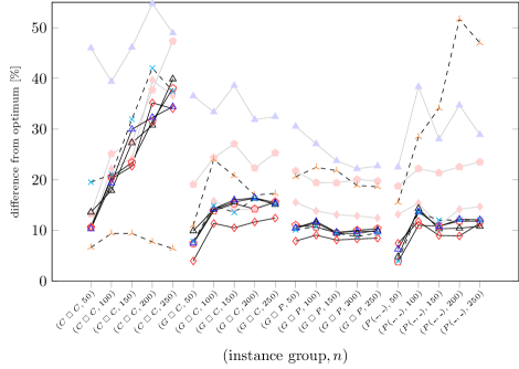
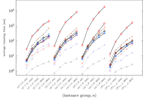
Figure 4: Comparison of the srm-variants on the KnownCR instances. The legend of Figure 5 applies. Instance sizes are rounded up to the nearest multiple of fifty. Note that the results of ccm-srm heavily depend on the structure of the instance; they also vary a lot across other instance sets (with middling results on average).

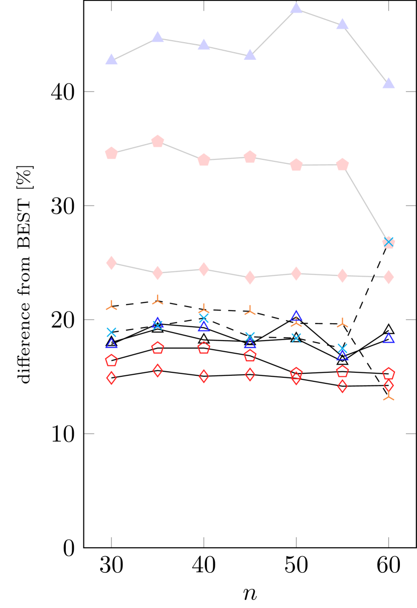
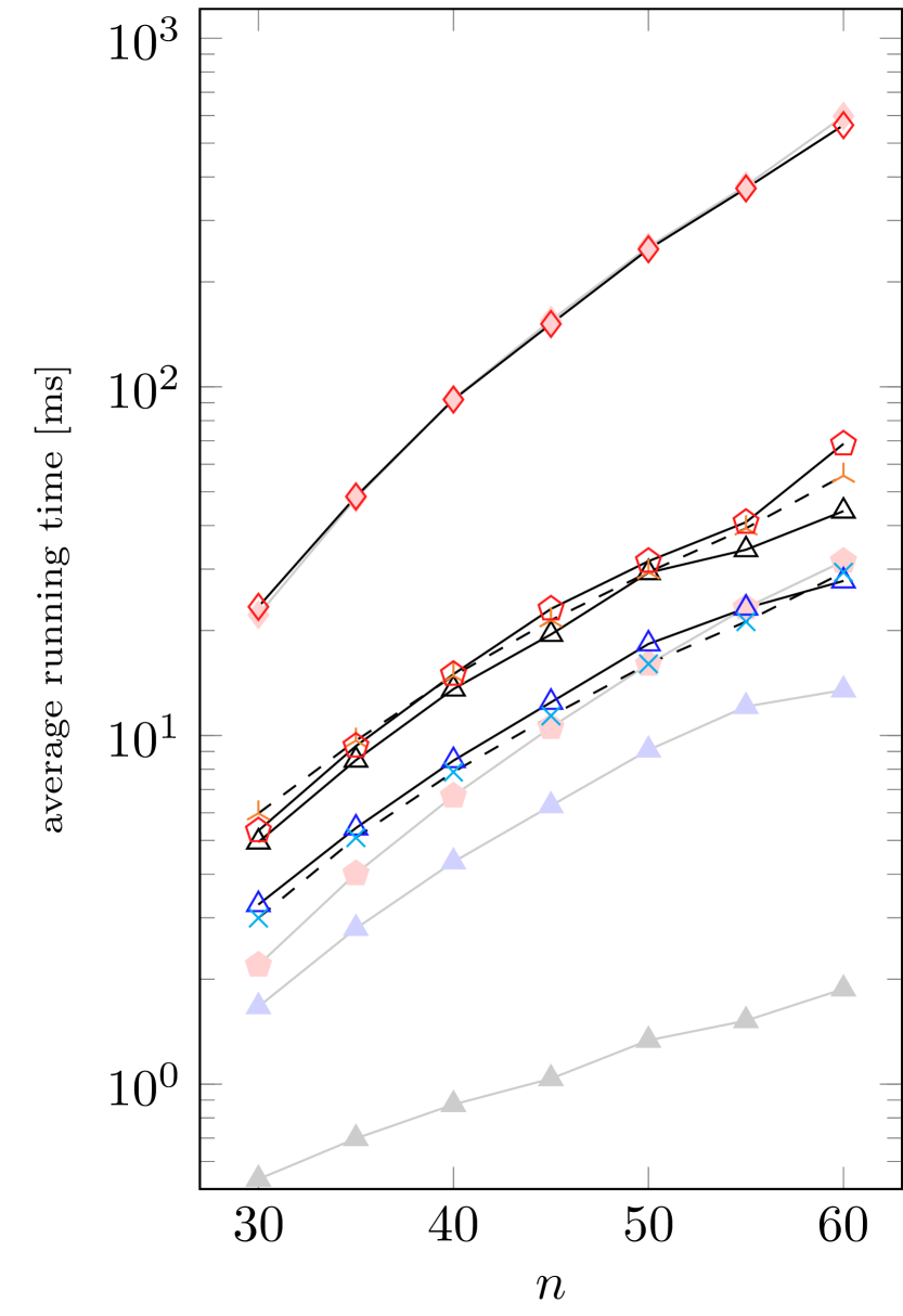
Figure 5: Comparison of the srm-variants on the Rome instances. The grayed out plots represent the heuristic variants without srm-postprocessing. Instance sizes are rounded up to the nearest multiple of five.

When observing the solution quality of the srm-algorithms, the same hierarchy as for the algorithms without srm emerges: fix-none-srm performs worse than the other plm-based srm-variants, with var-inc-srm providing the best results overall. However, var-inc-srm is rarely worth the additional running time since the three significantly faster mim-srm, ccm-srm and fix-none-srm perform similarly well or even surpass it on many instances such as several circuit-based ones and the expanders. In comparison to mim-srm for example, var-inc-srm’s solution quality difference to BEST is only 1.7% smaller but its median running time is eight times higher (when averaged over all instances). The running times of the faster algorithms seem to coincide with the quality of the planarization delivered by the base algorithm: While fix-none-srm is generally faster than ccm-srm on sparse instances, the opposite is true on denser ones. On complete (bipartite) instances, ccm-srm becomes even faster than mim-srm. However, mim-srm is the otherwise fastest among these algorithms, and thus we recommend to use it.

5.4 Improvements via Permutations

We will consider one last question: Whether multiple runs of the same algorithm with different random permutations of the inserted elements can significantly improve the results. For plm, we permute the order in which the deleted edges are inserted, and for mim, ccm and srm, we permute the order of (re)inserted stars. Our experiments compare the effect of 50 random permutations with respect to the Rome, North, Webcompute and KnownCR instance sets. For the larger instances and more time-consuming algorithms, this number of permutations is the limit of what we are able to compute. We focus on the (relative) improvement for each instance, i.e., the lowest number of crossings divided by the average number of crossings across 50 permutations (cf. Appendix 0.D).

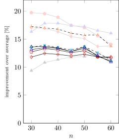
(a) Rome

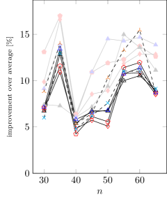
(b) North

Figure 6: Comparison of relative improvements for 50 permutations over their average on the Rome and North instances. The legend of Figure 5 applies.

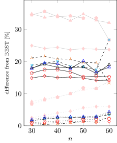
(a) Rome

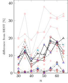
(b) North

Figure 7: Comparison of high-solution-quality heuristics (with a single or 50 permutations) on the Rome and North instances.

Overall, permutations can significantly improve the results of mim, ccm, and plm-none at the cost of little additional time. However, when more time is available, plm with postprocessing is clearly preferable. Multiple permutations of all and inc can be of use if one tries to marginally improve already good solutions. Among the srm-algorithms, the relative improvement via permutations is consistently low with little variance; for a comparison with the respective plm-variants see Figure 6. The one outlier is ccm-srm, which achieves the greatest relative improvements for 50 permutations. Note, however, that we initialize all permutations of ccm-srm with a fixed small chordless cycle instead of a fixed maximal planar subgraph. This allows for greater variance in the solutions of ccm-srm and makes it difficult to compare the results to other srm-algorithms.

The general trend of high-solution-quality algorithms, taking multiple permutations into account, is shown in Figure 7: A single permutation of mim-srm or ccm-srm will yield better solutions than a plm-variant with incremental postprocessing (but no srm). Two layers of postprocessing, i.e., -all-srm or -inc-srm, improve the results even more. Solutions resulting from 50 permutations are in a tier of their own, with srm-heuristics achieving higher quality than those without. Overall, 50 permutations of mim-srm or ccm-srm provide some of the best results while taking a lot less time than other algorithms in their category. Consider, e.g., the Rome instances in a 50-permutations setting; var-inc-srm can reduce the average solution quality difference to BEST by only 1.2% more than mim-srm, but its median running time is ten times as high.

6 Conclusion

Our in-depth experimental evaluation not only corroborates the results of previous papers [10, 17] but also provides new insights into the performance of star insertion in crossing minimization heuristics. We presented the novel heuristic mim, which proceeds similarly to the planarization method but inserts most edges by reinserting one of their endpoints as a star. Whenever neither endpoint is a cut vertex of the initial planar subgraph, the endpoint can be chosen freely, and our experiments indicate that reinserting both endpoints one after another provides the best results. In general, mim performs better than the basic heuristics from [10, 17] that have a similarly low running time (i.e., ccm and fix-none).

A central observation is that postprocessing via star insertion (srm) can greatly improve the planarizations resulting from fast heuristics: mim-srm, ccm-srm, and fix-none-srm are all faster than the previously best-performing heuristic var-inc and provide better results. By inserting multiple adjacent edges at once, star (re-)insertion changes the planarization and its underlying graph decomposition in a way that is sufficient to properly explore the search space and find good solutions. Fixed embedding star insertion is thus preferable over the much slower insertion of edges (or even stars) in a variable embedding setting.

We note that many heuristics—in particular those without edge-wise postprocessing—are prone to create non-simple crossings (due to lack of space see Appendix 0.C). Such crossings can be detected and it is worthwhile to remove them in order to speed up the procedure and improve the results. Lastly, multiple permutations are beneficial for heuristics that already employ postprocessing. In particular, their application to mim-srm and ccm-srm provides very high solution quality at moderate running times.

Appendix 0.A Statistics on Instance Sets

Figures 8–11 give an overview of the size of the instances mentioned in Section 5, including the number of edges that are deleted to create the planar subgraph. The plots also display the number of these deleted edges that are incident to one or two cut vertices of the planar subgraph as these are of particular relevance for the mixed insertion method (see Subsection 3.2). For plots over $n$ or the density of the instance, points for the x-axis values $x$, $y$ and $z$ represent the mean over all instances with x-axis values in the intervals $(0,x]$, $(x,y]$ and $(y,z]$.

Figure 8: Legend for plots displaying instance statistics.

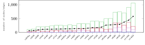
(a) ISCAS-89

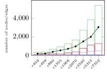
(b) ISCAS-85

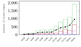
(c) ITC-99

Figure 9: Statistics on circuit-based instances.

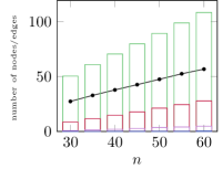
(a) Rome

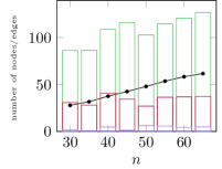
(b) North

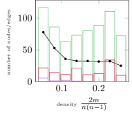
(c) Webcompute

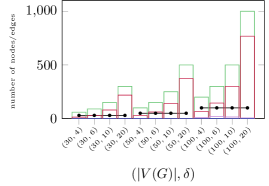
(d) Expanders

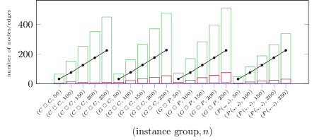
(e) KnownCR

Figure 10: Statistics on other instances.

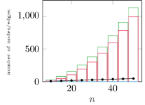
(a) Complete

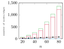
(b) Complete-Bip.

Figure 11: Statistics on complete (bipartite) instances.

Appendix 0.B Planarization Method

This appendix provides an extended version of Subsection 5.2. Figure 12 showcases the results and running times on the ISCAS-89 instances, on which plm has not been evaluated so far.

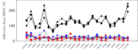
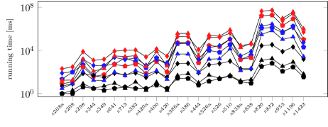
Figure 12: Comparison of the plm-variants on the ISCAS-89 instances. The instances s820 and s832 could not be solved with fix-inc due to the enforced memory limit.

One major insight is that (incremental) postprocessing via all or inc is a very worthwhile endeavour: In terms of solution quality, none provides much worse results than all and inc across all instance sets. While the switch from none to all causes a large jump in solution quality, the improvement of inc in comparison to all is smaller. The best results are usually provided by var-inc, with multi-inc being a close runner-up. However, inc has the drawback of very high running times and a large amount of required memory. Several circuit-based instances as well as many expanders with $|V(G)|\in\{50,100\},\delta=20$ could not be solved due to the enforced memory limit. For this reason, we did not even attempt to solve the complete (bipartite) instances with inc.

Furthermore, for each of the three postprocessing settings, there is a general trend among the edge insertion algorithms: Due to its search across all possible embeddings, var performs better than multi, which in turn performs better than fix. This overall hierarchy is especially evident (across all instance sets) when no postprocessing is employed. On the Rome instances it also persists for all and inc respectively. For other instance sets, the all-variants and fix-inc produce planarizations of intermediate quality, but which of these algorithms performs best depends on the instance. Here, the prowess of multi shines through: multi-all comes close to the solution quality of var-all and sometimes even surpasses it, as is the case on complete instances. For KnownCR, multi-all even trumps fix-inc.

When it comes to running times, var is the slowest edge insertion algorithm as it builds up a new SPR-tree after each edge insertion, and postprocessing takes a lot of additional time (inc especially so). In some cases, more involved postprocessing can be counter-balanced by employing fixed embedding edge insertion. Thus, fix-all is faster than var-none on the expanders, KnownCR, and Webcompute instances; and fix-inc is faster than var-all on Rome and larger KnownCR instances. Overall, fix-all is the fastest plm-variant that still benefits from the quality improvements of postprocessing.

However, the central observation is the speed of multi, which matches the speed of fix in many cases. On all instance sets except for Rome, multi-none becomes even faster than fix-none when considering larger instances. Furthermore, multi-inc is faster than fix-inc for Rome, Webcompute, the circuit-based instances, and dense expanders. This might be explained by the fact that intermediate planarizations produced by multi contain less crossings and that there is hence less computational overhead. As our implementation of multi performs incremental postprocessing in a fixed embedding setting, multi-inc also has a speed advantage over var-all and even multi-all (which uses postprocessing in a variable embedding setting) on a limited number of sparse instances. While multi does not lead to the best results (this is achieved by var-inc), it constitutes the best compromise between solution quality and speed.

Appendix 0.C Removal of Non-simple Crossings

To gain insight into the effectiveness of the removal of non-simple crossings, we counted how many of them were detected during each algorithm run. As one would expect, they occur primarily on dense instances, i.e., dense expanders and complete (bipartite) instances. When inspecting the final planarizations produced by plm, it becomes evident that in most cases, the postprocessing strategies all and inc already remove all non-simple crossings. In fact, on KnownCR instances, not a single such crossing can be found in the final solutions. When no postprocessing is used, however, we found (and removed) such crossings for 1027–1159 of all instances, with fix-none producing more of them than multi-none and var-none. A maximum of 3410 non-simple crossings was created during the run of fix-none on $K_{39,39}$.

For mim and ccm, we examine the sum of non-simple crossings found and removed after the reinsertion of each star. In comparison to plm without postprocessing, these numbers are considerably lower, presumably because inserting multiple edges via star insertion reduces the likelihood of producing such crossings. In particular, when inserting a star as described in Subsection 3.1, it is not possible to introduce a non-simple crossing between its edges. For mim, there are 517–855 affected instances overall (depending on the variant), with a maximum of 1916 non-simple crossings for $K_{40,40}$. While ccm results in similarly high numbers (543 instances), the corresponding distribution of non-simple crossings among the instance sets is striking: The algorithm does not produce any such crossings on complete (bipartite) instances but showcases a high occurrence rate on circuit-based instances, expanders and especially KnownCR. The numbers hence coincide with the performance of ccm on the respective instances.

With respect to the srm-postprocessing, we count only the non-simple crossings that are removed during the star reinsertion process, with those of the initial planarization being already removed. It can be observed that the totals depend heavily on the quality of the initial planarization—presumably because the creation of a non-simple crossing requires a specific configuration of already existing crossings (cf. Figure 1). Among srm-algorithms whose initial planarization is constructed using all or inc, fix-all-srm is the only one with more than 100 instances being affected by non-simple crossings during the star reinsertion phase (121 instances). For the remaining srm-algorithms, these numbers are considerably higher: fix-none-srm results in the highest amount of affected instances (1094), closely followed by ccm-srm (1024), with mim-srm producing roughly half as many (536).

In summary, the removal of non-simple crossings can significantly improve the final results of heuristics that do not employ any kind of postprocessing. It can also slightly improve intermediate planarizations during srm, potentially speeding up the procedure. However, with more involved postprocessing, non-simple crossings are less likely to occur, and their removal is hence less effective.

Appendix 0.D Relative Improvement via Permutations

Table 2 lists the average relative improvements of 50 permutations in comparison to the average permutation for each of the heuristics and instance sets mentioned in Subsection 5.4.

Table 2: Average relative improvement of 50 permutations compared to the average permutation in percent.

Algorithm	Rome	North	KnownCR	Webcompute
fix-none	10.60	9.57	4.91	7.60
fix-all	17.20	11.98	7.28	12.39
fix-inc	18.65	12.46	9.99	15.23
multi-none	13.66	11.95	6.14	10.50
multi-all	18.10	12.83	7.87	13.23
multi-inc	19.08	12.98	10.00	14.28
var-none	12.62	11.14	4.95	9.84
var-all	18.44	12.83	8.64	14.08
var-inc	16.57	11.46	8.48	12.43
mim	14.73	12.83	9.41	14.05
ccm	34.13	27.28	27.77	33.16
fix-none-srm	13.49	8.80	5.32	8.90
fix-all-srm	13.23	9.25	5.02	8.13
multi-all-srm	12.84	8.31	5.29	7.52
multi-inc-srm	12.93	8.93	6.72	6.90
var-all-srm	13.08	8.94	5.31	7.69
var-inc-srm	12.12	8.45	6.50	6.45
mim-srm	13.59	8.77	5.63	7.81
ccm-srm	16.88	11.03	15.19	10.38

References

- [1] Batini, C., Talamo, M., Tamassia, R.: Computer aided layout of entity relationship diagrams. J. Syst. Softw. 4(2-3), 163–173 (1984), https://doi.org/10.1016/0164-1212(84)90006-2
- [2] Battista, G.D., Garg, A., Liotta, G., Parise, A., Tamassia, R., Tassinari, E., Vargiu, F., Vismara, L.: Drawing directed acyclic graphs: An experimental study. Int. J. Comput. Geom. Appl. 10(6), 623–648 (2000), https://doi.org/10.1142/S0218195900000358
- [3] Battista, G.D., Garg, A., Liotta, G., Tamassia, R., Tassinari, E., Vargiu, F.: An experimental comparison of four graph drawing algorithms. Comput. Geom. 7, 303–325 (1997), https://doi.org/10.1016/S0925-7721(96)00005-3
- [4] Brglez, F., Bryan, D., Kozminski, K.: Notes on the ISCAS’89 benchmark circuits. Tech. rep., North-Carolina State University (Oct 1989)
- [5] Brglez, F., Fujiwara, H.: A neutral netlist of 10 combinational circuits and a targeted translator in FORTRAN. In: Proc. ISCAS; Special Session on ATPG and Fault Simulation. pp. 151–158 (Jun 1985)
- [6] Buchheim, C., Chimani, M., Ebner, D., Gutwenger, C., Jünger, M., Klau, G.W., Mutzel, P., Weiskircher, R.: A branch-and-cut approach to the crossing number problem. Discret. Optim. 5(2), 373–388 (2008), https://doi.org/10.1016/j.disopt.2007.05.006
- [7] Cabello, S., Mohar, B.: Crossing number and weighted crossing number of near-planar graphs. Algorithmica 60(3), 484–504 (2011), https://doi.org/10.1007/s00453-009-9357-5
- [8] Chalermsook, P., Schmid, A.: Finding triangles for maximum planar subgraphs. In: Proc. WALCOM 2017. LNCS, vol. 10167, pp. 373–384. Springer (2017), https://doi.org/10.1007/978-3-319-53925-6_29
- [9] Chimani, M., Gutwenger, C.: Non-planar core reduction of graphs. Discret. Math. 309(7), 1838–1855 (2009), https://doi.org/10.1016/j.disc.2007.12.078
- [10] Chimani, M., Gutwenger, C.: Advances in the planarization method: Effective multiple edge insertions. J. Graph Algorithms Appl. 16(3), 729–757 (2012), https://doi.org/10.7155/jgaa.00264
- [11] Chimani, M., Gutwenger, C., Jünger, M., Klau, G.W., Klein, K., Mutzel, P.: The Open Graph Drawing Framework (OGDF). In: Handbook on Graph Drawing and Visualization, pp. 543–569. Chapman and Hall/CRC (2013)
- [12] Chimani, M., Gutwenger, C., Mutzel, P.: Experiments on exact crossing minimization using column generation. ACM J. Exp. Algorithmics 14 (2009), https://doi.org/10.1145/1498698.1564504
- [13] Chimani, M., Gutwenger, C., Mutzel, P., Wolf, C.: Inserting a vertex into a planar graph. In: Proc. SODA 2009. pp. 375–383. SIAM (2009), http://dl.acm.org/citation.cfm?id=1496770.1496812
- [14] Chimani, M., Hlinený, P.: A tighter insertion-based approximation of the crossing number. J. Comb. Optim. 33(4), 1183–1225 (2017), https://doi.org/10.1007/s10878-016-0030-z
- [15] Chimani, M., Mutzel, P., Bomze, I.M.: A new approach to exact crossing minimization. In: Proc. ESA 2008. LNCS, vol. 5193, pp. 284–296. Springer (2008), https://doi.org/10.1007/978-3-540-87744-8_24
- [16] Chimani, M., Wiedera, T.: An ILP-based proof system for the crossing number problem. In: Proc. ESA 2016. LIPIcs, vol. 57, pp. 29:1–29:13 (2016), https://doi.org/10.4230/LIPIcs.ESA.2016.29
- [17] Clancy, K., Haythorpe, M., Newcombe, A.: An effective crossing minimisation heuristic based on star insertion. J. Graph Algorithms Appl. 23(2), 135–166 (2019), https://doi.org/10.7155/jgaa.00487
- [18] Corno, F., Reorda, M.S., Squillero, G.: RT-level ITC’99 benchmarks and first ATPG results. IEEE Des. Test Comput. 17(3), 44–53 (2000), https://doi.org/10.1109/54.867894
- [19] Garey, M.R., Johnson, D.S.: Crossing number is NP-complete. SIAM Journal on Algebraic Discrete Methods 4(3), 312–316 (1983)
- [20] Gutwenger, C.: Application of SPQR-Trees in the Planarization Approach for Drawing Graphs. Ph.D. thesis, TU Dortmund, Dortmund, Germany (2010), http://hdl.handle.net/2003/27430
- [21] Gutwenger, C., Mutzel, P.: An experimental study of crossing minimization heuristics. In: GD 2003: Revised Papers. LNCS, vol. 2912, pp. 13–24. Springer (2003), https://doi.org/10.1007/978-3-540-24595-7_2
- [22] Gutwenger, C., Mutzel, P., Weiskircher, R.: Inserting an edge into a planar graph. Algorithmica 41(4), 289–308 (2005), https://doi.org/10.1007/s00453-004-1128-8
- [23] Hlinený, P.: Crossing number is hard for cubic graphs. J. Comb. Theory, Ser. B 96(4), 455–471 (2006), https://doi.org/10.1016/j.jctb.2005.09.009
- [24] Hopcroft, J.E., Tarjan, R.E.: Efficient algorithms for graph manipulation [H] (algorithm 447). Commun. ACM 16(6), 372–378 (1973), https://doi.org/10.1145/362248.362272
- [25] Karp, R.M.: Reducibility among combinatorial problems. In: Complexity of Computer Computations. pp. 85–103. The IBM Research Symposia Series, Plenum Press, New York (1972), https://doi.org/10.1007/978-1-4684-2001-2_9
- [26] Steger, A., Wormald, N.C.: Generating random regular graphs quickly. Combinatorics, Probability and Computing 8(4), 377–396 (1999), https://doi.org/10.1017/S0963548399003867
- [27] Ziegler, T.: Crossing minimization in automatic graph drawing. Ph.D. thesis, Saarland University, Saarbrücken, Germany (2001), http://d-nb.info/961610808