Towards Memory-Efficient Neural Networks
via Multi-Level in situ Generation

Abstract

Deep neural networks (DNN) have shown superior performance in a variety of tasks. As they rapidly evolve, their escalating computation and memory demands make it challenging to deploy them on resource-constrained edge devices. Though extensive efficient accelerator designs, from traditional electronics to emerging photonics, have been successfully demonstrated, they are still bottlenecked by expensive memory accesses due to tremendous gaps between the bandwidth/power/latency of electrical memory and computing cores. Previous solutions fail to fully-leverage the ultra-fast computational speed of emerging DNN accelerators to break through the critical memory bound. In this work, we propose a general and unified framework to trade expensive memory transactions with ultra-fast on-chip computations, directly translating to performance improvement. We are the first to jointly explore the intrinsic correlations and bit-level redundancy within DNN kernels and propose a multi-level in situ generation mechanism with mixed-precision bases to achieve on-the-fly recovery of high-resolution parameters with minimum hardware overhead. Extensive experiments demonstrate that our proposed joint method can boost the memory efficiency by 10-20$\times$ with comparable accuracy over four state-of-the-art designs, when benchmarked on ResNet-18/DenseNet-121/MobileNetV2/V3 with various tasks.

1 Introduction

Deep neural networks (DNNs) have demonstrated record-breaking performance in a variety of intelligent tasks. Modern DNN models and datasets keep growing rapidly, which demonstrate critical conflicts with resource-constrained applications. Stringent constraints in efficiency, latency, and power in practical applications raise a surging need to develop more efficient computing solutions.

Extensive efficient neural network (NN) accelerators have been designed to support such domain-specific computations. In electrical domain, hardware-efficient digital platforms have been demonstrated, e.g., Eyeriss [5, 6], EIE [19], TPU [26]. Due to the high efficiency of analog computing, electrical analog accelerators gain much momentum recently, e.g., ReRAM-crossbar-based matrix multiplication engines [41, 45, 49]. As a promising substitute for electrical designs to continue Moore’s law, optical computing provides order-of-magnitude higher efficiency than electrical counterparts. In optical computing domain, photonic accelerators are proposed to provide considerably more efficient solutions to AI acceleration [43, 33, 61, 44, 58, 37, 12, 14, 15, 47, 35, 16, 13, 51, 42].

However, memory performance turns out to be the critical bottleneck since it fails to match the computing capability of emerging cores. Especially for emerging accelerators, e.g., ReRAM-based and photonics-based engines, the enormous latency, power, and bandwidth gap between memory and computing engines severely prohibits the full utilization of their advanced computing power.

Previous efforts towards memory-efficient accelerator designs focus on weight quantization [60, 38, 20], pruning with sparsity exploration [30, 20, 21, 50, 55, 9], structured weight matrices [11, 31, 14, 49], slim architectures [25, 7, 2], better hardware scheduling [34, 56], low-rank approximation [10, 46, 30, 57, 54, 53], etc. However, limited research has been done to thoroughly investigate the intrinsic redundancy in CNN kernels. It is in high demand to provide a unique memory optimization strategy that fully exploits the potentials of advanced ultra-fast AI acceleration platforms.

Therefore, in this work, we propose a unified framework that generalizes prior low-rank solutions for memory-efficient NN designs via a multi-level in situ weight generation technique with mixed-precision quantization. We are the first to jointly explore multi-level redundancy in channel, kernel, and bitwidth based on a strong intuition on the intrinsic correlations within convolutions. A photonic case study of in situ weight generator is presented to show how our method can help unleash the full power of emerging neuromorphic computing systems. The main contributions of this work are as follows,

• We explore the multi-level intrinsic correlation in CNNs and propose a unified framework that generalizes prior low-rank-based convolution designs for higher memory efficiency.

• We fully-leverage the ultra-fast execution speed of emerging accelerators and propose a hardware-aware multi-level in situ generation to trade expensive memory access for much cheaper computations.

• We integrate a precision-preserving mixed-precision strategy to leverage the bit-level redundancy in multi-level bases for a larger design space exploration.

• Experiments and a photonic case study show that our proposed multi-level in situ generation and mixed-precision techniques can save $\sim$97% weight load latency and significantly reduce memory cost by 10-20$\times$ with competitive accuracy compared to prior methods, even on compact networks and complex tasks.

2 Preliminary

In this section, we give a brief introduction to the background knowledge and our motivation.

2.1 Memory bottleneck in NN accelerator designs

Previous works have proposed extensive NN accelerator architectures to enable efficient DNN inference. Recent emerging non-Von Neumann accelerators mainly focus on the innovation of the core matrix multiplication engine. However, the computation speed and efficiency of the cores are no longer the bottlenecks of the overall system. To prove this claim, Figure 1d shows that multiple cascaded small convolutional layers have less floating-point operations (FLOPs) than a single wide convolutional layer but have higher execution time due to lower parallelism and more memory transactions. Hence, the expensive memory transaction and interconnect delay turn out to the pain point.

Most accelerators still rely on on-chip SRAMs and off-chip DRAMs to store/access weights, bringing serious challenges regarding the significant data movement cost. First, the mismatch between memory and computing cores in terms of latency and bandwidth heavily limits the potential performance of modern accelerators, especially for ultra-fast optical accelerators. Typical DRAM and SRAM has an access time of tens of nanoseconds, and the fastest SRAM runs at only 5 GHz. However, for example, the computation is executed at the speed of light (picosecond-level delay) in optical NNs with massive parallelism and potentially over 100 GHz photo-detection rate [43, 1].

Furthermore, data movement becomes the power bottleneck. Figure 1a shows the power breakdown on a recent photonic neural chip Mars [37, 48]. The SRAM access dominates the total power consumption. The same issue also exists in state-of-the-art (SOTA) electrical digital accelerators like famous Eyeriss [5, 6] shown in Figure 1b.

Limited prior works have explicitly optimized memory cost for emerging accelerators by leveraging their ultra-fast computing speed. Hence, a specialized memory-efficient NN design methodology to minimize data movement cost is exciting and essential to explore.

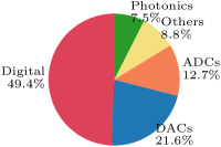
(a)

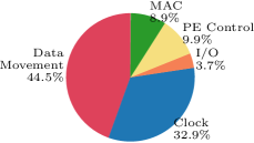
(b)

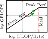
(c)

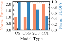
(d)

Figure 1:  Power breakdown of a silicon photonic accelerator Mars [37, 48] (a) and an electrical accelerator Eyeriss [5] (b). The data movement (red) takes the most power for both. (c) Roofline model of emerging accelerators. Memory-bounded designs (red point) need to be improved to a better design (green point) (d) Normalized runtime and number of floating-point operations (FLOPs) among different convolution (Conv) types. C5 is 5$\times$5 Conv, C5G is 5$\times$5 Conv with low-rank decomposition, 2C3 is two cascade 3$\times$3 Conv, and 4C1 is four cascade 1$\times$3 Conv.

2.2 Efficiency and accuracy trade-off

Extensive works have been done to explore the NN design space for higher efficiency with less accuracy degradation. Efficient neural architectures are designed with lightweight structures, e.g., depthwise separable convolution [7], blueprint convolution [18], channel shuffling [25], etc. Besides, network compression techniques are often utilized to explore the sparsity and redundancy of DNNs and trim the model size by pruning and quantization [21, 20]. Furthermore, low-rank decomposition [30, 57] is a widely adopted technique to reduce the number of parameters by approximating a weight matrix by two smaller matrices. Also, structured neural networks[14][15][31] have been proposed to reduce memory cost with block-circulant matrix representation and Fourier-transform-based algorithm.

The above generic methods are applicable for emerging ultra-fast neuromorphic engines but do not fully leverage their powerful computing capability. It will be interesting and promising to explore the intrinsic correlation in DNN weights and enable in situ weight generation by the computing core itself to minimize data movement from memory.

3 Proposed NN design methodology

Motivated by prior work [30, 57, 7, 18], we focus on widely deployed convolutional neural networks (CNNs) to thoroughly explore their intrinsic multi-level redundancy for better efficiency. We consider a 2-dimensional (2-D) convolutional kernel $\bm{W}\in\mathbb{R}^{C_{o}\times C_{i}\times k\times k}$ with $C_{o}$ kernels, $C_{i}$ input channels, and kernel sizes $k$. Interestingly we observe intrinsic multi-level correlation within the kernel that we can leverage for memory compression. This memory compression directly translates to latency/power improvement since convolutions have frequent weight access, whose memory cost is even higher than feature maps [4].

3.1 Multi-level weight generation

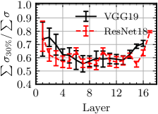
(a)

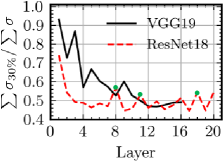
(b)

Figure 2:  Convolutional kernel correlations in ImageNet-pretrained models are shown by the proportion of the sum of the top 30% singular values ($\sum\sigma_{30\%}$). (a) Intra-kernel correlations averaged on different kernels. Error bars show the $\pm\sigma$ variance. We skip 1$\times$1 Conv. (b) Cross-kernel correlations, where green dots are 1$\times$1 Conv.

3.1.1 Intra-kernel correlation

We first explore the low-rank property among different channels of a kernel. The $i$-th kernel $\bm{W}_{i}\in\mathbb{R}^{C_{i}\times k^{2}}$ can be treated as a matrix with $C_{i}$ row vectors with length $k^{2}$. From its singular values $\bm{\Sigma}=\texttt{SVD}(\bm{W}_{i})=\texttt{diag}(\sigma_{0},\sigma_{1},\cdots)$, we observe relatively strong correlations between those column vectors since the first several major components $\sigma_{30\%}$ concentrates the majority of the total values. Figure 2a shows the intra-kernel low-rank property of modern CNNs. Different layers tend to have different intra-kernel correlations, where shallower layers show higher correlations. This provides us an opportunity to generate the $i$-th kernel $\bm{W}_{i}\in\mathbb{R}^{C_{i}\times k^{2}}$ using a low-dimensional channel basis $\bm{W}^{b}_{i}\in\mathbb{R}^{B_{i}\times k^{2}}$ with a cardinality of $B_{i}<\min(C_{i},k^{2})$ and a corresponding coefficient matrix $\bm{U}_{i}\in\mathbb{R}^{C_{i}\times B_{i}}$. Figure 3 visualizes the procedure for convolutions with a general matrix multiplication (GEMM) interpretation using the im2col algorithm [3]. This intra-kernel generation is formally expressed as.

$$\small\bm{W}_{i}=\bm{U}_{i}\bm{W}_{i}^{b},\quad\forall i\in[C_{o}]$$ (1)

Therefore, we reduce the parameter of the $i$-th kernel from $|\bm{W}_{i}|=C_{i}k^{2}$ to $|\bm{W}_{i}^{b}|+|\bm{U}_{i}|=B_{i}k^{2}+C_{i}B_{i}$. Note that for 1$\times$1 convolution, we skip this intra-kernel generation and directly use all $C_{i}$ channels given the constraint $B_{i}<\min(C_{i},1^{2})$.

3.1.2 Cross-kernel correlation

Furthermore, we explore the second-level correlation cross $C_{o}$ kernels. We view the entire convolutional kernel $\bm{W}\in\mathbb{R}^{C_{o}\times(C_{i}k^{2})}$ as a matrix with $C_{o}$ row vectors with length of $C_{i}k^{2}$. Figure 2b quantifies the correlation among different kernels. Though it is slightly weaker than the intra-kernel correlation, it still brings another opportunity to further decompose the weight along another dimension. Instead of generating $C_{o}$ kernels independently, we only generate a subset of kernels as our kernel basis $\bm{W}_{c}=\{\bm{W}_{i}\in\mathbb{R}^{C_{i}k^{2}},\forall i\in[B_{c}],B_{c}<\min(C_{o},C_{i}k^{2})\}$ using Eq. (1). This generated kernel basis $\bm{W}_{c}$ is used to span the entire kernel together with another coefficient matrix $\bm{V}\in\mathbb{R}^{C_{o}\times B_{c}}$ as follows,

$$\small\bm{W}=\bm{V}\bm{W}_{c}=\bm{V}\{\bm{U}_{i}\bm{W}_{i}^{b}\}_{i\in[B_{c}]},$$ (2)

If $B_{c}\geq\min(C_{o},C_{i}k^{2})$, we only consider intra-kernel correlation by setting $B_{c}=C_{o}$ without performing Equation (2). After the proposed two-level generation, the parameter compression ratio is,

$$r= \frac{|\bm{V}|+\sum_{i\in[B_{c}]}(|\bm{U}_{i}|+|\bm{W}_{i}^{b}|)}{|\bm{W}|}=\frac{\big{(}C_{o}+B_{i}k^{2}+C_{i}B_{i}\big{)}B_{c}}{C_{o}C_{i}k^{2}}.$$ (3)

The extra computation for in situ kernel generation $\mathcal{O}(2B_{c}C_{i}B_{i}k^{2}+2C_{o}B_{c}C_{i}k^{2})$ is marginal compared with the convolution itself $\mathcal{O}(2C_{o}C_{i}k^{2}HW)$, where $H$ and $W$ are output feature map sizes. Thus the runtime overhead is negligible, consistent with what we showed before in Figure 1d. In this way, we successfully save expensive memory transactions with marginal computation overhead, which fully leverages the emerging accelerators’ ultra-fast computing capability to mitigate the critical memory bound.

3.2 Augmented mixed-precision generation

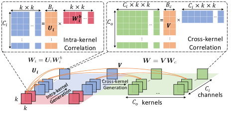
Figure 3:  Intra-kernel and cross-kernel generation.

Besides the weight correlation that explores parameter-level reduction, we further explore the bit-level redundancy with mixed-precision bases. Modern NN accelerator designs, especially emerging analog engines, prefer to use low-bit weights to reduce memory access latency and simplify the control circuitry complexity [60, 38, 43, 17, 59]. In this section, we utilize the precision preserving feature of analog engines and propose an augmented mixed-precision generation strategy to recover high-precision weights with low-bitwidth basis and coefficients.

We assume the bitwidths for $\bm{W}^{b}_{i}$, $\bm{U}_{i}$, and $\bm{V}$ are $q_{b}$, $q_{u}$, and $q_{v}$, respectively. The first-level intra-kernel generation is capable of generating $\bm{W}_{c}\in\mathbb{R}^{B_{c}\times(C_{i}k^{2})}$ with at most $(2^{q_{b}}-1)(2^{q_{u}}-1)B_{i}+1$ possible distinct values, which corresponds to a bitwidth upper bound $\sup(q_{c})=(q_{b}+q_{u}+\log_{2}{B_{i}})$. Unlike digital cores, this precision can be maintained by the direct cascade of two analog tensor units without resolution loss caused by the analog-to-digital conversion. Then, the cross-kernel generator will output $\bm{W}$ with an equivalent bitwidth $\sup(q)=(q_{v}+\sup(q_{c})+\log_{2}{B_{o}})$ that can also be preserved in the matrix multiplication unit. The advantages are clear that our method enables the weight generator to be completely in the analog domain to recover a high-precision, i.e., $q>q_{b},q_{u},q_{v}$, weight matrix using low-precision basis and coefficient matrices. The memory compression ratio $r_{m}$ is thus calculated as,

$$r_{m} =\frac{\sum_{i\in[B_{c}]}\big{(}q_{b}|\bm{W_{i}}^{b}|+q_{u}|\bm{U}_{i}|\big{)}+q_{v}|\bm{V}|}{q_{w}|\bm{W}|}$$ (4)

$$=\frac{B_{c}B_{i}k^{2}q_{b}+B_{c}C_{i}B_{i}q_{u}+C_{o}B_{c}q_{v}}{C_{o}C_{i}k^{2}q_{w}}.$$

Hence, given a target $q_{w}$, we can explore fine-grained mixed-precision settings of $q_{b}$, $q_{u}$, and $q_{v}$ to further cut down the memory cost in the bit-level, which is an orthogonal technique to the above parameter-level counterparts.

3.3 Training with in situ weight generation

Algorithm 1 Training with in situ generation

1:A pretrained teacher $\widehat{\mathcal{M}}$ with weights $\widehat{\bm{W}}$, a student model $\mathcal{M}$ with $\bm{W}^{b}_{i}$, $\bm{U}_{i}$, and $\bm{V}$, mixed-precision bitwidths $q_{b}$, $q_{u}$, and $q_{v}$, training dataset $\mathcal{D}^{trn}$, total iterations $T$, initial step size $\eta^{0}$;

2:Converged student model;

3:$\text{Step 1:~{}}\ell_{2}\text{~{}Initialization from the teacher model}$

4:$\bm{W}^{b}_{i},\bm{U}_{i},\bm{V}\leftarrow\operatorname*{argmin}~{}\|\widehat{\bm{W}}-\bm{V}\{\bm{U}_{i}\bm{W}_{i}^{b}\}_{i\in[B_{c}]}\|_{2}^{2}$

5:Step 2: Quantization-aware knowledge distillation

6:for $t\leftarrow 0\cdots T-1$ do

7:    Randomly sample a mini-batch $\mathcal{I}^{t}$ from $\mathcal{D}^{trn}$

8:    $\bm{U}_{i}^{t+1}\leftarrow\bm{U}_{i}^{t}-\eta^{t}\nabla_{\bm{U}_{i}}(\mathcal{L}_{KD}+\lambda\mathcal{L}_{ort}),~{}\forall i\in[B_{c}]$

9:    $\bm{W}_{i}^{b,t+1}\leftarrow\bm{W}_{i}^{b,t}-\eta^{t}\nabla_{\bm{W}^{b}_{i}}(\mathcal{L}_{KD}+\lambda\mathcal{L}_{ort}),~{}\forall i\in[B_{c}]$

10:    $\bm{V}^{t+1}\leftarrow\bm{V}^{t}-\eta^{t}\nabla_{\bm{V}_{i}}(\mathcal{L}_{KD}+\lambda\mathcal{L}_{ort})$

11:    $\eta^{t+1}=\texttt{Update}(\eta^{t})$ $\triangleright$ Step size decay

Our main target is to reduce memory cost with acceptable accuracy loss. Now we introduce how to optimize the designed CNN with in situ generators such that the desired accuracy can be achieved. We adopt a two-stage quantization-aware knowledge distillation to train our proposed NN, described in Alg. 1. Firstly, we obtain a pre-trained full-precision model without in situ generation as our teacher model $\widehat{\mathcal{M}}$ whose weight matrix is denoted as $\widehat{\bm{W}}$. Our low-rank mixed-precision model is the corresponding student model $\mathcal{M}$ whose weight matrix $\bm{W}$ is generated by quantized $\bm{W}_{i}^{b}$, $\bm{U}_{i}$, and $\bm{V}$. A differentiable quantizer [60] is used in our quantization-aware training. For simplicity, we omit the quantization notation for quantized $\bm{W}_{i}^{b}$, $\bm{U}_{i}$, and $\bm{V}$ if mixed-precision quantization is used. Then we let the student mimic the teacher using a two-stage training algorithm. First, we solve the following problem to project the teacher model onto the student parameter space by minimizing their $\ell_{2}$ distance,

$$\small\min~{}\|\widehat{\mathcal{M}}(\widehat{\bm{W}})-\mathcal{M}(\bm{W})\|_{2}^{2}\approx\|\widehat{\bm{W}}-\bm{V}\{\bm{U}_{i}\bm{W}_{i}^{b}\}_{i\in[B_{c}]}\|_{2}^{2}.$$ (5)

Given the smoothness of $\mathcal{M}$ and $\widehat{\mathcal{M}}$, the above $\ell_{2}$ distance can be approximated by the first-order term of its Taylor expansion. This $\ell_{2}$ distance-based subspace projection is an effective and efficient initialization method for the student model. Then we try to find local optima in the low-rank space starting from this projected solution point. Therefore, in the second stage, we train the student model with knowledge distillation [23] as,

$$\min{} \mathcal{L}_{KD}=\beta T^{2}\mathcal{D}_{KL}(q_{T},p_{T})+(1-\beta)H(q,p_{T=1}),$$ (6)

s.t. $$p_{T}=\frac{\exp(\frac{\mathcal{M}(\bm{W})}{T})}{\sum\exp(\frac{\mathcal{M}(\bm{W})}{T})},q_{T}=\frac{\exp(\frac{\widehat{\mathcal{M}}(\widehat{\bm{W}})}{T})}{\sum\exp(\frac{\widehat{\mathcal{M}}(\widehat{\bm{W}})}{T})},$$

$$\bm{W}=\bm{V}\{\bm{U}_{i}\bm{W}_{i}^{b}\}_{i\in[B_{c}]},$$

$$0<B_{i}<\min(C_{i},k^{2}),B_{i}\in\mathbb{Z}$$

$$0<B_{c}<\min(C_{o},C_{i}k^{2}),B_{i}\in\mathbb{Z},$$

where $\mathcal{M}(\bm{W})$ is the output logits, $\mathcal{D}_{KL}$ is the Kullback–Leibler divergence between two probability distributions, $H(\cdot,\cdot)$ is the cross entropy, $q$ is the ground truth distribution, $T$ and $\beta$ are hyper-parameters controlling the smoothness. This training method [23] can distill the representability of the high-rank full-precision model to our low-rank quantized student.

However, we notice that once the basis and coefficient matrices have a deficient row-rank or column-rank, the spanning subspace of the generated matrix will become too small to approximate the original full-rank matrix. Therefore, to maximize the rank of the spanned weight matrix, we set a row orthonormality constraint to the basis $\bm{W}^{b}_{i}$ and a column orthogonality constraint to the coefficient matrices. This constraint can be relaxed using penalty methods as a multi-level orthogonal regularization term $\mathcal{L}_{ort}$ as follows,

$$\sum_{i=1}^{B_{c}}\!\Big{(}\|\bm{W}^{b}_{i}(\bm{W}^{b}_{i})^{T}\!-\!\bm{I}\|_{2}^{2}\!+\!\|\tilde{\bm{U}}_{i}^{T}\tilde{\bm{U}}\!-\!\bm{I}\|_{2}^{2}\Big{)}\!+\!\|\tilde{\bm{V}}^{T}\tilde{\bm{V}}\!-\!\bm{I}\|_{2}^{2},$$ (7)

$$\tilde{\bm{U}}_{i}=\begin{pmatrix}\frac{u_{0}}{\|u_{0}\|_{2}^{2}}&\!\!\!\!\cdots\!\!\!\!&\frac{u_{0}}{\|u_{B_{i}-1}\|_{2}^{2}}\end{pmatrix},\tilde{\bm{V}}=\begin{pmatrix}\frac{v_{0}}{\|v_{0}\|_{2}^{2}}&\!\!\!\!\cdots\!\!\!\!&\frac{v_{0}}{\|v_{B_{c}-1}\|_{2}^{2}}\end{pmatrix}.$$

Equation (7) is a generalization to a previous single-level penalty [18, 54] and exerts a soft constraint to multi-level correlations such that the spanning space will not collapse to a low-dimensional subspace. Therefore, the overall loss function is $\mathcal{L}=\mathcal{L}_{KD}+\lambda\mathcal{L}_{ort}$.

3.4 Case study: silicon photonics implementation

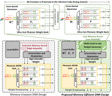
Figure 4:  Photonic implementation of in situ weight generator and peripheral structures. Left bottom

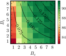
(a)

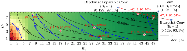
(b)

Figure 5:  (a) Accuracy (color) and compression ratio (contour) of the customized 3-layer CNN on FashionMNIST [52] with various $B_{i}$ and $B_{c}$ (92.14% Acc. for the original Conv). (b) Accuracy (blue contour) and compression ratio $r$ (black contour) for ResNet-18 on CIFAR-10. Red stars are representative settings of our method. Blue stars show previous designs.

We showcase a photonic implementation of the proposed in situ weight generator in Figure 4. We focus on a SOTA design based on micro-ring resonators [47]. Other accelerators can also benefit from our method as long as the multi-level correlation and precision preserving properties hold.

After loading the lightweight basis and coefficient matrices from the local electrical buffer, two cascaded ultra-fast optical weight banks will achieve the first-level and second-level generation to obtain the final weights $\bm{W}$. Without intermediate storage, the analog weights are directly broadcast to all photonic tensor units via ultra-low-power optical interconnects [1] to perform the primary operation, e.g., convolution. Compared with the memory-agnostic design, which requires massive and frequent weight loading, our proposed design can effectively cut down memory footprint and access latency. Consider a 16-bit ($q_{w}$=16) kernel $\bm{W}\in\mathbb{R}^{128\times 128\times 3\times 3}$ and a setting ($B_{i},B_{c},q_{b},q_{u},q_{v}$)=(2,40,4,4,4) implemented by micro-rings of diameter $R$=20 $\upmu$m, the extra latency introduced by in situ generator is as follows,

$$\tau_{gen} =(\tau_{DAC}+\tau_{mod}+\tau_{prop1}+\tau_{oe})+(\tau_{mod}+\tau_{prop2}+\tau_{oe})$$ (8)

$$\approx\tau_{DAC}+2\times(\tau_{mod}+\tau_{oe})+\frac{4B_{i}R}{c}+\frac{4B_{c}R}{c}$$

$$\approx 400~{}\text{ps}+2\times(50~{}\text{ps}+10~{}\text{ps})+25.2~{}\text{ps}=545.2~{}\text{ps}$$

$$\ll\frac{2(1-r_{m})|\bm{W}|}{BW_{SRAM}}\!\approx\!\frac{(1-0.0272)\times 288~{}\text{KB}}{34~{}\text{GB/s}}=7.9~{}\text{$\upmu$s},$$

where $\tau_{DAC}$ is the latency for 10 Gb/s digital-to-analog converter, $\tau_{mod}$ is the device modulation delay, $\tau_{prop}$ is the photonic weight bank propagation delay, $\tau_{oe}$ is the optical-to-electrical conversion delay for layer cascade, $c$ is the light speed, and $BW_{SRAM}$ is the SRAM bandwidth [26]. The generator saves 7.9 $\upmu$s latency ($>$97% of total weight load latency) with merely 545.2 ps weight generation latency overhead. Given $\sim$50% of total latency is consumed by kernel loading [4], our weight generation leads to at least 2$\times$ overall speedup. More speedup can be expected if activation quantization is further applied. In terms of power, our method can achieve significant energy reduction since we save $(1-r_{m})\approx 97\%$ weight loading and replace all high-resolution DACs with $(1-r)\approx 89\%$ fewer low-bit DACs [39] (power is exponential to bitwidth), which account for most power as shown in Figure 1a.

We further perform quantitative evaluation on a neuromorphic simulator MNSIM-2.0. On ResNet-18/ImageNet, compared with 8-bit BSConv, our method reduces the overall latency from 56.46 ms to 41.11 ms (27.2%$\downarrow$), reduces the overall energy from 25.77 mJ to 3.69 mJ (85.7%$\downarrow$), and improves energy-delay-product by 9.6$\times$.

4 Experiments

In this section, we first conduct ablation experiments on the proposed techniques and compare our method with prior efficient designs in memory cost and accuracy.

4.1 Dataset

Our ablation and comparison experiments are based on FashionMNIST [52], CIFAR-10 [29], and CIFAR-100. We also test on more tasks including SVHN [36], TinyImagetNet-200 [8], StanfordDogs-120 [27] and StandfordCars-196 [28] for fine-grained classification.

4.2 Neural network architectures

We first use a customized 3-layer CNN as a toy example to do multi-level correlation exploration on FashionMNIST, whose settings are (C32K5S2-C32K5S1-C32K5S1-AvgPool3-FC10), where C32K5S2 is a 5$\times$5 convolution with 32 kernels and stride 2, AvgPool3 is an average pooling layer with output size 3$\times$3, and FC10 means the output linear layer. BatchNorm and ReLU activation are used between convolutional layers. Then, the rest ablation experiments and comparison experiments are based on ResNet-18  [22], DenseNet-121  [24], and MobileNetV2 [40], which are adapted to CIFAR-10/100.

4.3 Training settings

We train all models for 200 epochs using RAdam [32] optimizer with an initial learning rate of 0.002, an exponential decay rate of 0.98 per epoch, and a weight decay of 5e-4. On CIFAR-10/100, images are augmented by random horizontal flips and random crops with 4 paddings. On TinyImageNet, StanfordDogs-120, and StanfordCars-196, additional color jitter is added. Mini-batch sizes are 64, 128, 64, and 64 for our 3-layer CNN, ResNet-18, DenseNet-121, and MobileNetV2, respectively.

4.4 Ablation: multi-level correlation exploration

To explore the impact of the multi-level basis cardinality $B_{i}$ and $B_{c}$ on the parameter count and accuracy, we first perform a grid search on FashionMNIST with our customized 3-layer CNN, shown in Figure 5a. In terms of parameter compression ratio $r$, $B_{c}$ shows a stronger impact than $B_{i}$ since $r\propto B_{c}$ while $B_{i}$ only partially contributes to $r$. For test accuracy, generally larger $B_{i}$ and $B_{c}$ lead to higher accuracy. However, the accuracy is much more sensitive to $B_{c}$ than $B_{i}$, where we find a great opportunity to minimize memory cost with a small accuracy drop. Therefore, we conclude a heuristic design guidance that a small $B_{i}$ and medium $B_{c}$ leads to sweet points. We further validate it on CIFAR-10 with ResNet-18, whose contours are shown in Figure 5b. In the design space exploration, we also plot full-rank Conv, depthwise separable Conv [22], and blueprint Conv [18] as our special cases. The blueprint Conv can be generalized by our method once $B_{i}$=1 and $B_{c}$=max. To some extent, separable Conv can also be generalized by setting $B_{i}$=max and $B_{c}$=1 while using different $\bm{V}$ for different input channels. Note that sharing $\bm{V}$ across channels is the key-point for our efficiency superiority. With the concluded design guidance, we indeed can quickly find design points that outperform the above prior works in memory efficiency with comparable accuracy, e.g., ($B_{i}$=2, $B_{c}$=44). Note that we assume a global ($B_{i}$, $B_{c}$) setting for all layers, while layer-specific cardinalities can be an interesting future topic to push towards the Pareto front.

4.5 Ablation: multi-level orthogonality regularization

Several representative ($B_{c}$,$B_{i}$) pairs are evaluated on ResNet-18 CIFAR-10 with various regularization weights $\lambda$. Figure 6 reveals that the model performance can be consistently improved by 0.5%-1% with proper $\lambda$ values ($0.01\sim 0.05$). This shows that the proposed multi-level orthogonal penalty term can encourage the spanned kernel to be as high-rank as possible with augmented representability.

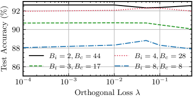
Figure 6:  Exploration on different orthogonal regularization weights with ResNet-18 on CIFAR-10[29].

	Param Ratio $r$=0.025				Param Ratio $r$=0.05
	$B_{i}$	$B_{c}$	$B_{i}$	$B_{c}$	$B_{i}$	$B_{c}$	$B_{i}$	$B_{c}$
	3	17	8	8	2	44	4	28
Baseline	90.62%		88.02%		92.46%		91.98%
Ortho Reg	90.82%		88.52%		92.88%		92.32%
SVD Init	91.32%		88.10%		93.05%		92.80%
$\ell_{2}$ Init	91.32%		88.85%		93.18%		92.75%
$\ell_{2}$+Ortho	91.40%		88.65%		93.17%		92.93%
$\ell_{2}$+Ortho+KD	91.52%		88.96%		93.29%		93.19%

Table 1:  Accuracy evaluation on orthogonal regularization (Ortho), initialization ($\ell_{2}$ and SVD), and knowledge distillation (KD). ResNet-18 is evaluated on CIFAR-10.

4.6 Ablation: initialization and distillation

We further evaluate different combinations of the proposed $\ell_{2}$ initialization and knowledge distillation with representative ($B_{i},B_{c}$) pairs in Table. 1. In our $\ell_{2}$ initialization, we optimize Equation (5) using RAdam [32] for 3k iterations with lr=2e-2. We first compare with a traditional truncated singular value decomposition (SVD) based method [10, 54]. Both methods benefit accuracy while our $\ell_{2}$ initialization demonstrates better results. With orthogonality penalty and knowledge distillation ($\beta$=0.9, $T$=3), our method achieves the highest accuracy. In conclusion, a good initialization and knowledge from the teacher are critical to the accuracy of the student model.

4.7 Ablation: mixed-precision bases exploration

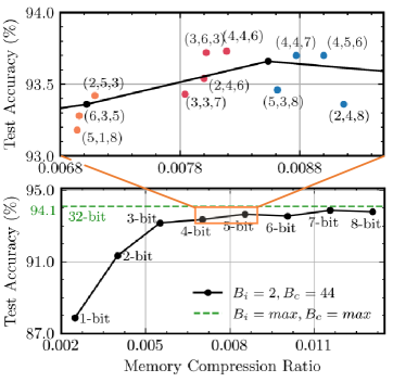
Figure 7:  Accuracy and memory compression ratio contour of ResNet-18 on CIFAR-10 with mixed-precision quantization ($q_{b},q_{u},q_{v}$). Black dots show $q_{b}$=$q_{u}$=$q_{v}$.

	CIFAR-10			CIFAR-100
	Param Ratio	Mem Ratio	Acc	Param Ratio	Mem Ratio	Acc
ResNet-18 (Conv) [22]	1.0000	1.0000	94.10%	1.0000	1.0000	73.53%
ResNet-18 (DSConv) [7]	0.1287	0.1287	92.10%	0.1323	0.1323	68.65%
ResNet-18 (PENNI d=2) [30]	0.2352	0.2352	92.77%	0.2383	0.2383	70.14%
ResNet-18 (BSConv) [18]	0.1291	0.1291	93.10%	0.1327	0.1327	71.11%
ResNet-18 (CirCNN k=4) [11]	0.2510	0.2510	92.16%	0.2541	0.2541	67.93%
ResNet-18 (Ours-2-44-32-32-32)	0.0497	0.0497	93.29%	0.0536	0.0536	70.85%
ResNet-18 (Ours-2-44-8-8-8)	0.0497	0.0131	93.79%	0.0536	0.0140	71.05%
ResNet-18 (Ours-2-44-3-6-3)	0.0497	0.0080	93.72%	0.0536	0.0090	71.47%
DenseNet-121 (Conv) [24]	1.0000	1.0000	94.69%	1.0000	1.0000	76.51%
DenseNet-121 (DSConv) [7]	0.7362	0.7362	93.81%	0.7396	0.7396	74.35%
DenseNet-121 (PENNI d=2) [30]	0.7608	0.7608	94.32%	0.7640	0.7640	75.26%
DenseNet-121 (BSConv) [18]	0.7291	0.7291	94.24%	0.7326	0.7326	75.79%
DenseNet-121 (CirCNN k=4) [11]	0.2601	0.2601	92.86%	0.2698	0.2698	72.45%
DenseNet-121 (Ours-1-25-32-32-32)	0.1986	0.1986	94.89%	0.2091	0.2091	75.09%
DenseNet-121 (Ours-1-25-8-8-8)	0.1986	0.0587	94.78%	0.2091	0.0612	75.59%
DenseNet-121 (Ours-1-25-4-6-6)	0.1986	0.0395	94.68%	0.2091	0.0422	75.05%

Table 2: Comparison among efficient convolutions in terms of parameter/memory compression ratio (smaller is better) and accuracy. The cardinality $d$ in PENNI is 2. CirCNN uses a block size $k$=4. (Ours-$B_{i}$-$B_{c}$-$q_{b}$-$q_{u}$-$q_{v}$) is the network setup.

We perform a fine-grained investigation on the mixed-precision bitwidth $(q_{b},q_{u},q_{v})$ to justify the trade-off between accuracy and memory efficiency. For simplicity, we assume the same bitwidth combination for all layers. Figure 7 plots the accuracy-memory curve with equal $q_{b}$, $q_{u}$, and $q_{v}$. Above 3-bit, we can maintain over 93% accuracy ($\sim$1% drop). Equal bit-precision for basis and coefficients may not be the best combination. Thanks to our mixed-precision bit-level generation mechanism, we allow larger freedom to further explore different $q_{b}$, $q_{u}$, and $q_{v}$ settings around a region of interest where the accuracy starts to drop. One key observation is that mixed-precision settings indeed can lead to higher accuracy with lower memory cost than equal settings. We also observe that relatively-balanced settings, e.g., (2,5,3), (4,5,6), generally outperform extremely-imbalanced ones, e.g., (5,1,8), (2,4,8). Hence, we claim that relatively-balanced mixed-precision bases are preferred to achieve better memory efficiency and less accuracy loss.

4.8 Comparison with prior work

Our method can serve as a memory-efficient drop-in substitution for normal convolutions. To show the superiority of our method over prior arts, we compare the memory compression ratio and inference accuracy with the baseline convolution (Conv) and four representative prior works, depthwise separable Conv (DSConv) [22], single-level low-rank decomposition (PENNI) [30], blueprint Conv (BSConv) [18], and block-circulant Conv (CirCNN) [11] on ResNet-18 and DenseNet-121 in Table. 2. For fair comparisons, all methods only apply to convolutional layers and use the same training settings as mentioned. To clarify, the selection of ($B_{i}$,$B_{c}$,$q_{b}$,$q_{u}$,$q_{v}$) is not from exhaustive enumeration but simply based on the target compression ratio and the heuristic design guidance we concluded. We only evaluate the unpruned PENNI version since pruning is an orthogonal technique to our method. We use a low-rank factor $d$=2 for PENNI [30] and a circulant block size $k$=4 for CirCNN [11] for a comparable memory cost and accuracy.

Compared with the baseline convolution, our 32-bit version achieves 5$\times$-20$\times$ memory reduction. Compared with our special cases DSConv and BSConv, our method with a small $B_{i}$ and a medium $B_{c}$ shows 2$\times$-4$\times$ memory reduction and comparable accuracy. Our multi-level generation outperforms the single-level low-rank decomposition method PENNI with 3.8$\times$-4.7$\times$ lower memory cost and better accuracy. We outperform CirCNN in both metrics. With mixed-precision generation, we boost the memory efficiency by 25$\times$-125$\times$ and 16$\times$-19$\times$ over the baseline Conv and the best prior work BSConv respectively, with competitive accuracy. Though on DensetNet-121 CIFAR-100, we have $\sim$0.7% accuracy drop, we have much lower memory cost. A larger $B_{c}$ and higher bitwidths can be selected to recover the accuracy as a trade-off.

4.9 Boost compact models on harder tasks

To fully justify our superiority, we need to answer another three important questions: 1) how does it perform on architectures that are already compact; 2) is it compatible with activation quantization that is more memory bottlenecked; and 3) does the compressed low-rank kernel still have enough representability to capture critical features in high-resolution images. Similar to Figure 2, we also observe strong intra-kernel correlation for depth-wise Conv (DWConv) and cross-kernel correlation for point-wise Conv (PWConv). Hence we further apply our in-situ generation scheme to each individual DWConv and PWConv in the inverted residual block of MobileNet-V2 for further weight compression. Besides, we perform quantization to activation for each layer to save the most critical activation memory cost. Table 3 shows that we can further save $>$10$\times$ weight storage and reduce the largest activation memory cost by 4$\times$ even on compact architectures. On fine-grained image recognition tasks where the input images have high resolutions and low categorical variances, the compressed models still demonstrate strong model representability that can capture subtle but critical traits with negligible accuracy drop. Table 4 evaluates our methods further on searched compact networks on detection tasks, which are known to be energy/memory-demanding, our method can lead to 5-12$\times$ compression with marginal performance loss.

	CIFAR-10		CIFAR-100
	Mem Ratio	Acc	Mem Ratio	Acc
Original [40]	1.0000	93.06%	1.0000	73.90%
Ours-5-40-4-4-4	0.0783	94.03%	0.0867	73.11%
Ours-5-40-4-4-4 (A8)	0.0783	94.02%	0.0867	72.90%
	SVHN		TinyImageNet-200†
Original [40]	1.0000	96.37%	1.0000	67.13%
Ours-5-40-4-4-4	0.0783	96.61%	0.1251	65.59%
Ours-5-40-4-4-4 (A8)	0.0783	96.63%	0.1251	65.44%
	StanfordDogs-120†		StanfordCars-196†
Original [40]	1.0000	72.25%	1.0000	89.32%
Ours-5-40-4-4-4	0.0885	71.06%	0.0948	89.54%
Ours-5-40-4-4-4 (A8)	0.0885	71.42%	0.0948	89.47%

Table 3: In-situ generation with activation/weight quantization on MobileNetV2 [40]. The setup follows (Ours-$B_{i}$-$B_{c}$-$q_{b}$-$q_{u}$-$q_{v}$). A8 means 8-bit activation. ^† means teacher models are initialized with ImageNet-pretrained models. The setup for TinyImageNet is (6-60-5-5-5).

	StanfordDogs-120		ImageNet-50		PASCAL VOC
	Mem Ratio	Acc	Mem Ratio	Acc	Mem Ratio	mAP
MobilenetV2 (SSD-lite)	1.0000	72.25%	1.0000	87.56%	1.0000	0.683
Ours (SSD-lite)	0.0885	71.06%	0.0821	87.52%	0.1392	0.655
MobilenetV3-S (SSD-lite)	1.0000	65.41%	1.0000	85.04%	1.0000	0.544
Ours (SSD-lite)	0.2082	66.64%	0.2060	85.44%	0.2238	0.513
EfficientNet-B0	1.0000	75.43%	1.0000	89.56%	-	-
Ours	0.1257	75.00%	0.1132	88.52%	-	-

Table 4: Evaluate compact models beyond simple tasks and classification.

5 Conclusion

In this work, we propose a general and unified framework for memory-efficient DNN designs via multi-level in situ generation. We jointly leverage the intrinsic correlation and bit-level redundancy within convolutional kernels and allow the ultra-fast accelerator to generate the weights in situ by itself to boost the performance. A photonic case study is given to show our latency/power advantages. Experiments show that our method achieves 10$\times$-20$\times$ memory efficiency boost compared with prior methods. Our method provides a unified view to prior single-level low-rank methods and enables a new design paradigm to break through the ultimate memory bottleneck for emerging DNN accelerators by their tremendous computing power.

References

- [1] Liane Bernstein, Alexander Sludds, Ryan Hamerly, Vivienne Sze, Joel Emer, and Dirk Englund. Freely scalable and reconfigurable optical hardware for deep learning. ArXiv, abs/2006.13926, 2020.
- [2] Han Cai, Chuang Gan, Tianzhe Wang, Zhekai Zhang, and Song Han. Once for All: Train One Network and Specialize it for Efficient Deployment. In Proc. ICLR, 2020.
- [3] K. Chellapilla, Sidd Puri, and P. Simard. High performance convolutional neural networks for document processing. In Proc. ICFHR, 2006.
- [4] Y. Chen, J. Emer, and V. Sze. Eyeriss: A Spatial Architecture for Energy-Efficient Dataflow for Convolutional Neural Networks. In Proc. ISCA, pages 367–379, 2016.
- [5] Y. Chen, T. Krishna, J. Emer, and V. Sze. Eyeriss: An energy-efficient reconfigurable accelerator for deep convolutional neural networks. In Proc. ISSCC, pages 262–263, 2016.
- [6] Y. Chen, T. Krishna, J. S. Emer, and V. Sze. Eyeriss: An energy-efficient reconfigurable accelerator for deep convolutional neural networks. IEEE Journal Solid-State Circuits, 52(1):127–138, 2017.
- [7] François Chollet. Xception: Deep learning with depthwise separable convolutions. In Proc. CVPR, pages 1800–1807, 2017.
- [8] J. Deng, W. Dong, R. Socher, L.-J. Li, K. Li, and L. Fei-Fei. ImageNet: A Large-Scale Hierarchical Image Database. In Proc. CVPR, 2009.
- [9] Lei Deng, Guoqi Li, Song Han, Luping Shi, and Yuan Xie. Model compression and hardware acceleration for neural networks: A comprehensive survey. Proceedings of the IEEE, 2020.
- [10] Emily Denton, Wojciech Zaremba, Joan Bruna, Yann LeCun, and Rob Fergus. Exploiting Linear Structure Within Convolutional Networks for Efficient Evaluation . In Proc. NIPS, 2014.
- [11] Caiwen Ding, Siyu Liao, Yanzhi Wang, Zhe Li, Ning Liu, et al. CirCNN: Accelerating and Compressing Deep Neural Networks Using Block-Circulant Weight Matrices. In Proc. MICRO, pages 395–408, 2017.
- [12] Chenghao Feng, Zheng Zhao, Zhoufeng Ying, Jiaqi Gu, David Z. Pan, and Ray T. Chen. Compact design of On-chip Elman Optical Recurrent Neural Network. In Proc. CLEO, 2020.
- [13] Jiaqi Gu, Chenghao Feng, Zheng Zhao, Zhoufeng Ying, Mingjie Liu, Ray T. Chen, and David Z. Pan. SqueezeLight: Towards Scalable Optical Neural Networks with Multi-Operand Ring Resonators. In Proc. DATE, Feb. 2021.
- [14] Jiaqi Gu, Zheng Zhao, Chenghao Feng, et al. Towards area-efficient optical neural networks: an FFT-based architecture. In Proc. ASPDAC, 2020.
- [15] Jiaqi Gu, Zheng Zhao, Chenghao Feng, et al. Towards Hardware-Efficient Optical Neural Networks: Beyond FFT Architecture via Joint Learnability. IEEE TCAD, 2020.
- [16] Jiaqi Gu, Zheng Zhao, Chenghao Feng, Zhoufeng Ying, Ray T. Chen, and David Z. Pan. O2NN: Optical Neural Networks with Differential Detection-Enabled Optical Operands. In Proc. DATE, Feb. 2021.
- [17] Jiaqi Gu, Zheng Zhao, Chenghao Feng, Hanqing Zhu, Ray T. Chen, and David Z. Pan. ROQ: A noise-aware quantization scheme towards robust optical neural networks with low-bit controls. In Proc. DATE, 2020.
- [18] Daniel Haase and Manuel Amthor. Rethinking Depthwise Separable Convolutions: How Intra-Kernel Correlations Lead to Improved MobileNets. In Proc. CVPR, pages 14588–14597, 2020.
- [19] Song Han, Xingyu Liu, Huizi Mao, Jing Pu, Ardavan Pedram, Mark A. Horowitz, and William J. Dally. EIE: Efficient Inference Engine on Compressed Deep Neural Network. In Proc. ISCA, 2016.
- [20] Song Han, Huizi Mao, and William Dally. Deep compression: Compressing deep neural networks with pruning, trained quantization and huffman coding. In Proc. ICLR, 2016.
- [21] Song Han, Jeff Pool, John Tran, and William J. Dally. Learning both weights and connections for efficient neural networks. In Proc. NIPS, 2015.
- [22] Kaiming He, Xiangyu Zhang, Shaoqing Ren, and Jian Sun. Deep residual learning for image recognition. In Proc. CVPR, pages 770–778, 2016.
- [23] Geoffrey Hinton, Oriol Vinyals, and Jeff Dean. Distilling the knowledge in a neural network. arXiv preprint arXiv:1503.02531, 2015.
- [24] Gao Huang, Zhuang Liu, Laurens Van Der Maaten, and Kilian Q. Weinberger. Densely Connected Convolutional Networks. In Proc. CVPR, pages 2261–2269, 2017.
- [25] Forrest N. Iandola, Song Han, Matthew W. Moskewicz, Khalid Ashraf, William J. Dally, and Kurt Keutzer. SqueezeNet: AlexNet-level accuracy with 50x fewer parameters and¡ 0.5MB model size. In Proc. ICLR, 2017.
- [26] Norman P. Jouppi, Cliff Young, Nishant Patil, David Patterson, Gaurav Agrawal, Raminder Bajwa, et al. In-Datacenter Performance Analysis of a Tensor Processing Unit. In Proc. ISCA, 2017.
- [27] Aditya Khosla, Nityananda Jayadevaprakash, Bangpeng Yao, and Li Fei-Fei. Novel dataset for fine-grained image categorization. In Proc. CVPR, 2011.
- [28] Jonathan Krause, Michael Stark, Jia Deng, and Li Fei-Fei. 3D Object Representations for Fine-grained Categorization. In International IEEE Workshop on 3D Representation and Recognition (3dRR-13), 2013.
- [29] Alex Krizhevsky, Geoffrey Hinton, et al. Learning multiple layers of features from tiny images. 2009.
- [30] Shiyu Li, Edward Hanson, Hai Li, and Yiran Chen. PENNI: Pruned Kernel Sharing for Efficient CNN Inference . In Proc. ICML, 2020.
- [31] S. Liao, Z. Li, X. Lin, Q. Qiu, Y. Wang, and B. Yuan. Energy-efficient, high-performance, highly-compressed deep neural network design using block-circulant matrices. In Proc. ICCAD, pages 458–465, 2017.
- [32] Liyuan Liu, Haoming Jiang, Pengcheng He, Weizhu Chen, Xiaodong Liu, Jianfeng Gao, and Jiawei Han. On the variance of the adaptive learning rate and beyond. In Proc. ICLR, April 2020.
- [33] W. Liu, W. Liu, Y. Ye, Q. Lou, Y. Xie, and L. Jiang. Holylight: A nanophotonic accelerator for deep learning in data centers. In Proc. DATE, 2019.
- [34] Sangkug Lym, Armand Behroozi, Wei Wen, Ge Li, Yongkee Kwon, and Mattan Erez. Mini-Batch Serialization: CNN Training with Inter-Layer Data Reuse. In Proc. MLSys, 2017.
- [35] Mario Miscuglio and Volker J. Sorger. Photonic tensor cores for machine learning. Applied Physics Review, 2020.
- [36] Yuval Netzer, Tao Wang, Adam Coates, Alessandro Bissacco, Bo Wu, and Andrew Y. Ng. Reading Digits in Natural Images with Unsupervised Feature Learning. In Proc. NIPS, 2011.
- [37] Carl Ramey et al. Silicon photonics for artificial intelligence acceleration. In Proc. HotChips, 2020.
- [38] Mohammad Rastegari, Vicente Ordonez, Joseph Redmon, and Ali Farhadi. XNOR-Net: ImageNet Classification Using Binary Convolutional Neural Networks. In Proc. ECCV, pages 525–542, 2016.
- [39] M. Saberi, R. Lotfi, K. Mafinezhad, and W. A. Serdijn. Analysis of Power Consumption and Linearity in Capacitive Digital-to-Analog Converters Used in Successive Approximation ADCs. IEEE TCAS I, 58(8):1736–1748, 2011.
- [40] Mark Sandler, Andrew Howard, Menglong Zhu, Andrey Zhmoginov, and Liang-Chieh Chen. MobileNetV2: Inverted Residuals and Linear Bottlenecks. In Proc. CVPR, 2018.
- [41] A. Shafiee, A. Nag, N. Muralimanohar, R. Balasubramonian, J. P. Strachan, M. Hu, R. S. Williams, and V. Srikumar. ISAAC: A Convolutional Neural Network Accelerator with In-Situ Analog Arithmetic in Crossbars. In Proc. ISCA, pages 14–26, 2016.
- [42] Bhavin J. Shastri, Alexander N. Tait, T. Ferreira de Lima, Wolfram H. P. Pernice, Harish Bhaskaran, C. D. Wright, and Paul R. Prucnal. Photonics for artificial intelligence and neuromorphic computing. Nature Photonics, 2021.
- [43] Yichen Shen, Nicholas C. Harris, Scott Skirlo, et al. Deep learning with coherent nanophotonic circuits. Nature Photonics, 2017.
- [44] Kyle Shiflett, Dylan Wright, Avinash Karanth, and Ahmed Louri. PIXEL: Photonic Neural Network Accelerator. In Proc. HPCA, pages 474–487, 2020.
- [45] L. Song, X. Qian, H. Li, et al. Pipelayer: A pipelined reram-based accelerator for deep learning. In Proc. HPCA, 2017.
- [46] Cheng Tai, Tong Xiao, Yi Zhang, Xiaogang Wang, and Weinan E. Convolutional neural networks with low-rank regularization . In Proc. ICLR, 2016.
- [47] Alexander N. Tait, Thomas Ferreira de Lima, Ellen Zhou, et al. Neuromorphic photonic networks using silicon photonic weight banks. Sci. Rep., 2017.
- [48] A. R. Totović, G. Dabos, N. Passalis, A. Tefas, and N. Pleros. Femtojoule per MAC Neuromorphic Photonics: An Energy and Technology Roadmap. IEEE Journal of Selected Topics in Quantum Electronics, 26(5):1–15, 2020.
- [49] Yitu Wang, Fan Chen, Linghao Song, C.-J. Richard Shi, Hai Helen Li, and Yiran Chen. ReBoc: Accelerating Block-Circulant Neural Networks in ReRAM. In Proc. DATE, pages 1472–1477, 2020.
- [50] Wei Wen, Chunpeng Wu, Yandan Wang, Yiran Chen, and Hai Li. Learning structured sparsity in deep neural networks. In Proc. NIPS, 2016.
- [51] Gordon Wetzstein, Aydogan Ozcan, Sylvain Gigan, Shanhui Fan, Dirk Englund, Marin Soljačić, Cornelia Denz, , David A. B. Miller, and Demetri Psaltis. Inference in artificial intelligence with deep optics and photonics. Nature, 2020.
- [52] Han Xiao, Kashif Rasul, and Roland Vollgraf. Fashion-MNIST: a Novel Image Dataset for Benchmarking Machine Learning Algorithms. Arxiv, 2017.
- [53] Yuhui Xu, Yuxi Li, Shuai Zhang, Wei Wen, Botao Wang, Yingyong Qi, Yiran Chen, Weiyao Lin, and Hongkai Xiong. TRP: Trained Rank Pruning for Efficient Deep Neural Networks. In Proc. IJCAI, pages 977–983, 2020.
- [54] Huanrui Yang, Minxue Tang, Wei Wen, Feng Yan, Daniel Hu, Ang Li, Hai Li, and Yiran Chen. Learning low-rank deep neural networks via singular vector orthogonality regularization and singular value sparsification. In Proc. CVPR Workshops, 2020.
- [55] Tianyun Zhang, Shaokai Ye, Kaiqi Zhang, Jian Tang, Wujie Wen, Makan Fardad, and Yanzhi Wang. A systematic dnn weight pruning framework using alternating direction method of multipliers. In Proc. ECCV, 2018.
- [56] Zhekai Zhang, Hanrui Wang, Song Han, and William J. Dally. SpArch: Efficient Architecture for Sparse Matrix Multiplication. In Proc. HPCA, 2020.
- [57] Yang Zhao, Xiaohan Chen, Yue Wang, Chaojian Li, Haoran You, Yonggan Fu, Yuan Xie, Zhangyang Wang, and Yingyan Lin. SmartExchange: Trading Higher-cost Memory Storage/Access for Lower-cost Computation . In Proc. ISCA, 2020.
- [58] Zheng Zhao, Derong Liu, Meng Li, et al. Hardware-software co-design of slimmed optical neural networks. In Proc. ASPDAC, 2019.
- [59] Qilin Zheng, Zongwei Wang, Zishun Feng, Bonan Yan, Yimao Cai, Ru Huang, Yiran Chen, Chia-Lin Yang, and Hai Helen Li. Lattice: An ADC/DAC-less ReRAM-based Processing-In-Memory Architecture for Accelerating Deep Convolution Neural Networks. In Proc. DAC, pages 1–6, 2020.
- [60] Shuchang Zhou, Zekun Ni, Xinyu Zhou, He Wen, Yuxin Wu, and Yuheng Zou. Dorefa-net: Training low bitwidth convolutional neural networks with low bitwidth gradients. arXiv preprint arXiv:1606.06160, 2016.
- [61] Farzaneh Zokaee, Qian Lou, Nathan Youngblood, et al. LightBulb: A Photonic-Nonvolatile-Memory-based Accelerator for Binarized Convolutional Neural Networks. In Proc. DATE, 2020.