Unsupervised Reservoir Computing for Solving Ordinary Differential Equations

Abstract

There is a wave of interest in using unsupervised neural networks for solving differential equations. The existing methods are based on feed-forward networks, while recurrent neural network differential equation solvers have not yet been reported. We introduce an unsupervised reservoir computing (RC), an echo-state recurrent neural network capable of discovering approximate solutions that satisfy ordinary differential equations (ODEs). We suggest an approach to calculate time derivatives of recurrent neural network outputs without using backpropagation. The internal weights of an RC are fixed, while only a linear output layer is trained, yielding efficient training. However, RC performance strongly depends on finding the optimal hyper-parameters, which is a computationally expensive process. We use Bayesian optimization to efficiently discover optimal sets in a high-dimensional hyper-parameter space and numerically show that one set is robust and can be used to solve an ODE for different initial conditions and time ranges. A closed-form formula for the optimal output weights is derived to solve first order linear equations in a backpropagation-free learning process. We extend the RC approach by solving nonlinear system of ODEs using a hybrid optimization method consisting of gradient descent and Bayesian optimization. Evaluation of linear and nonlinear systems of equations demonstrates the efficiency of the RC ODE solver.

1 Introduction

Neural networks (NNs) have been widely applied recently to study various kinds of differential equations. Physics-informed NNs can be trained on data to learn nonlinear differential operators [1], discover differential equations [2, 3], and find approximate solutions for those equations [4]. These data-driven supervised networks have been applied to a variety of real-world problems such as learning the dynamics of mechanical systems [5, 6, 7] and designing meta-materials for nano-photonics [8]. Unsupervised NNs have been used to solve a variety of differential equations such as ordinary differential equations (ODEs) [9, 10, 11, 12], partial differential equations [13, 14, 15, 12], and eigenvalue problems [16]; these networks do not use any labeled data. Semi-supervised models have been applied to learn general solutions of differential equations and extract solutions which best fit given data [17]. Unsupervised NN solvers present exceptional advantages over traditional integrators: they suffer less from the "curse of dimensionality" in solving high-dimensional partial differential equations [13, 18], the numerical solutions are obtained in a closed and differentiable form [9], numerical errors are not accumulated in the solutions [12], initial and boundary conditions are identically satisfied [9, 16], and the solutions can be inverted [17, 8, 19]. Despite the success of the aforementioned models, all approaches are based on feed-forward NNs, while, to the best of our knowledge, recurrent neural networks (RNNs) for solving differential equations in an unsupervised fashion have not been reported yet. In this study, we fill the gap by introducing an unsupervised RNN, in the context of reservoir computing (RC) [20], which is able to discover approximate solutions to systems of ODEs.

RC is an echo state RNN where the internal parameters (weights and biases) are fixed, while only a linear output layer needs to be trained yielding fast and computationally efficient training [20, 21, 22]. Fixing the internal weights eliminates gradient exploding/vanishing problems during the training [20]. RC has been widely used for studying dynamical systems such as weather forecasting [23], predicting chaotic [21, 24] and irregular behavior [22], and classifying time series [25]. Moreover, the RC architecture has been adopted to build physical hardware NNs for neuromorphic computing [26, 27, 28, 29, 30, 31]. Neuromorphic devices are currently being developed for intelligent and energy-efficient devices providing extremely fast real-time computing with very low energy cost. This study suggests an avenue to design neuromorphic differential equation solvers.

The proposed RC solver is an extension to NN differential equation solvers and consequently, acquires all the benefits that network solvers have over numerical integrators. Moreover, RNNs perform better than feed-forward NNs on sequential data. Considering that the solutions of ODEs are time series and, therefore, similar to sequential data, we expect RNNs to generalize better than feed-forward NNs. The internal weights of an RC are fixed and randomly initialized from distributions that have certain statistical properties which yield the echo-state property [20, 21]. Training an RC is efficient, however, finding the optimal hyper-parameters that determine the weight distributions and the network architecture is challenging. RC performance strongly depends on these hyper-parameters and, therefore, finding good hyper-parameters is crucial. The RC has many hyper-parameters making this a computationally expensive process. Conventionally, simple grid-search in the hyper-parameter space is used [21], however, this method is prohibitively expensive for more than three hyper-parameters. Tuning hyper-parameters by using Bayesian Optimization (BO) is an active field of research [32, 33, 34, 35, 36]. In this study, we use TURBO-1, a BO method introduced in [33]. The strength of this method is discussed in the supplementary material (SM). We find that a single set of hyper-parameters is robust and can be used to solve ODEs for different initial conditions and time ranges.

Main contributions: First, in the continuous time limit we suggest an approximation to calculate time derivatives of the outputs of an RNN without using backpropagation, which is a substantial ingredient in ODE-solver neural networks. Second, we introduce an unsupervised RC and show that it is capable of solving ODEs. Third, we derive a closed-form formula for the RC trainable parameters for solving first order non-autonomous linear ODEs in a backpropagation-free learning method. Fourth, we develop a hybrid method consisting of gradient descent and BO which is able to find optimal hyper-parameters and weights of an RC for solving systems of nonlinear ODEs. For this study, we use the rcTorch library, an RC framework written in pytorch with embedded BO that utilizes BoTorch [36]. A public open-source github repository is available at https://github.com/blindedjoy/RcTorch.

2 Background: Neural network differential equations solvers

Several software libraries of NN differential equations solvers have been recently developed, including NeuroDiffEq [15], DeepXDE [37], and SimNet [38], indicating that developing NN solvers is an active area of research [39]. All of these libraries are based on feed-forward NNs and developed with the pytorch or tensorflow software platforms, where the automatic differentiation mechanism is employed to compute analytical derivatives used to define the loss function. In this context NN solvers are unsupervised learning methods. Since we want to solve differential equations, we do not know the corresponding target solutions and thus, we lack labeled or ground truth data. The only accessible information is the differential equation and the associated initial or boundary conditions. The loss function solely depends on the network predictions including the differential equation, while the initial/boundary conditions are embedded in the structure of the network and are thus identically satisfied. Neural network solvers are able to solve ordinary and partial differential equations of an arbitrary order. We nevertheless focus on ODEs in this study — particularly on systems of first order ODEs since higher order ODEs can be decomposed into systems of first order ODEs. We review here the approach of developing NNs for solving a first order ODEs subjected to certain initial conditions (ICs). Consider a general ODE of the form

$$D\left(t,\psi,\dot{\psi}\right)-f(t)=0,$$ (1)

where $t$ is the independent variable time, and $\psi(t)$ is the dependent variable subjected to a certain IC $\psi(0)=\psi_{0}$. In Eq. (1), $D$ is an arbitrary function of $\psi(t)$ and its first time derivative $\dot{\psi}$, and $f(t)$ is a forcing function of $t$. Equation (1) describes a non-autonomous system since it explicitly dependents on time. Considering known $D$ and $f$ functions, we are seeking $\psi(t)$ that solves Eq. (1) and satisfies a given $\psi_{0}$. Specifically, the goal is to construct a numerical solution $y$ which approximates the unknown ground truth solution $\psi$. To achieve that, we employ a NN that takes an input $t=(t_{1},t_{2},\dotsc,t_{K})$ and returns an output $N(t,p)$; $K$ indicates the total number of the input data points, and $p$ denotes the trainable parameters of the network. An efficient way to impose ICs was introduced in Ref. [9] and suggests using of a parametric solution $y(t)$ of the form:

$$y(t) =\psi_{0}+g(t)N(t,p)$$ (2)

where $g(t)$ can be any arbitrary function of $t$ with the constraint $g(0)=0$. The parametrization of Eq. (2) generates NN solutions that identically satisfy the ICs [9, 12, 10], namely $y(0)=\psi_{0}$. Having the parametric solution of Eq. (2), which is a function of $N$, solving the ODE of Eq. (1) is reduced to an optimization problem of the form

$$\underset{p}{\arg\min}\left(\sum_{n=0}^{K}\Big{(}D\left(t_{n},y_{n},\dot{y}_{n}\right)-f(t_{n})\Big{)}^{2}\right),$$ (3)

where $y_{n}=y(t_{n})$. The sum in Eq. (3) defines a loss function whose minimization yields $p$ that constructs a neural solution $y$ which approximately solves the ODE (1). It is worth noting that $y(t)$ can approximate $\psi(t)$ with arbitrary small error due to the universal approximation theorem of NNs [40]. Furthermore, regularization terms can be used to penalize large weights or to impose physical principles like energy conservation [12]. Subsequently, the total loss function is expressed as:

$$L =L_{\text{ODE}}+L_{\text{reg}}$$

$$=\sum_{n=0}^{K}\Big{(}D\left(t_{n},y_{n},\dot{y}_{n}\right)-f(t_{n})\Big{)}^{2}+L_{\text{reg}}.$$ (4)

The NN solution $y$ of Eq. (2) is a closed-form solution, meaning that it can be evaluated at every time point, differentiated, and inverted. These are unique properties of NN solvers that are not shared by standard integrators. Despite the advantages shown by feed-forward NN solvers, an RNN solver is missing from the literature. In this work, we present a novel RNN solver, specifically an echo-state RC, capable of solving ODEs in a given training and IC range.

3 Continuous-time recurrent neural networks

Learning from sequential data is a challenging task for machine learning because of the underlying time correlation. RNNs share parameters across the hidden layers giving them an intrinsic memory and subsequently, they are well suited to handle sequential data. Standard RNNs require discrete input data at discrete time points. In the continuous-time limit, when the discrete time points are close to each other, the dynamics of the hidden RNN layers can be approximated by continuously defined dynamics through ODEs [41, 42, 43]. This approximation has been adopted by residual networks [41] and continuous depth models [42, 43]. This is a core idea in the present study because it allows, in a backpropagation-free process, the calculation of the time derivatives of the outputs of an RNN.

Consider an RNN unit with $P$ input time series ${\bf u}(t)=(u_{1}(t),\dotsc u_{P}(t))\in{\rm I\!R}^{P}$, and $M$ hidden recurrent neurons described by a temporal state vector ${\bf h}(t)=(h_{1}(t),\dotsc h_{M}(t))\in{\rm I\!R}^{1\times M}$, where the time variable consists of $K$ points as $t=(t_{1},t_{2},\dotsc,t_{K})$. We show that in the continuous-time limit where the time step $\Delta t$ between two sequential data points is very small ($\Delta t\ll 1$), the dynamics of a leaky RNN unit can be approximated by a system of first order nonlinear ODEs of the form,

$$\dot{\bf h}=-\tilde{\alpha}{\bf h}+\tilde{\alpha}f\left({\bf W}_{\text{res}}\cdot{\bf h}+{\bf W}_{\text{in}}\cdot{\bf u}+{\bf b}\right),$$ (5)

where $\dot{\bf h}\equiv d{\bf h}/dt$ and the dot denotes the inner product. The input weights and biases are represented, respectively, by ${\bf W}_{\text{in}}\in{\rm I\!R}^{M\times P}$ and ${\bf b}\in{\rm I\!R}^{M}$, ${\bf W}_{\text{res}}\in{\rm I\!R}^{M\times M}$ describes the recurrent weights, $\tilde{\alpha}$ is the leakage rate, and $f(\cdot)$ denotes a nonlinear activation function [21]. Applying a Euler discretization for the first derivatives, $\dot{\bf h}=\frac{{\bf h}_{n+1}-{\bf h}_{n}}{\Delta t}$, the system of Eq. (5) takes the discrete form

$${\bf h}_{n+1}=\left(1-\alpha\right){\bf h}_{n}+\alpha f\left({\bf W}_{\text{res}}\cdot{\bf h}_{n}+{\bf W}_{\text{in}}\cdot{\bf u}_{n}+{\bf b}\right),$$ (6)

with $\alpha=\tilde{\alpha}\Delta t$. Equation (6) describes the update of a leaky RNN unit and subsequently, it is a first order approximation of the continuous model described by Eq. (5). Since Eq. (6) determines all ${\bf h}_{n}$ of an RNN, Eq. (5) provides, without any computational cost, the first time derivatives as:

$$\dot{\bf h}_{n}=-\frac{\alpha}{\Delta t}{\bf h}_{n}+\frac{\alpha}{\Delta t}f\left({\bf W}_{\text{res}}\cdot{\bf h}_{n}+{\bf W}_{\text{in}}\cdot{\bf u}_{n}+{\bf b}\right).$$ (7)

Higher order derivatives can be calculated by taking time derivatives of Eq. (7) and applying the chain rule to the $f(\cdot)$ term. The only numerical error in the first derivative of Eq. (7) is introduced through the assumption that Eq. (6) is derived from Eq. (5) by applying a Euler discretization. This error can be arbitrary small by appropriately choosing a small $\Delta t$. Consequently, the time derivatives of the hidden states can be estimated without using backpropagation.

Considering the general case of an RNN that returns $R$ outputs $N(t)\in{\rm I\!R}^{R}$, we read

$$N(t_{n})={\bf W_{o}}\cdot{\bf h}_{n}+{\bf b_{\text{o}}},$$ (8)

where ${\bf W_{o}}\in{\rm I\!R}^{R\times M}$ and ${\bf b_{\text{o}}}\in{\rm I\!R}^{R}$ are the weights matrix and biases of an output linear layer. The time derivative of $N$ can be calculated in a backpropagation-free mode using the result in Eq. (7) as:

$$\dot{N}(t_{n})={\bf W_{o}}\cdot\dot{\bf h}_{n}.$$ (9)

Backpropagating in RNNs is computationally expensive and can be impractical for large $K$. On the other hand, through Eq. (9) we can compute time derivatives without computational cost. Although throughout this study we apply Eqs. (7) and (9) for the RC architecture, the approach has broader implications since it holds for any RNN. Subsequently, it opens the door to a wide range of potential applications including general differential equation NN solvers and physics-informed RNNs.

4 Reservoir computing forms an ordinary differential equation solver

In this section, we introduce an unsupervised RC model that takes $t$ as an input sequence, namely ${\bf u}_{n}=t_{n}$, and is trained to solve ODEs within the range of $t$. First, we examine single linear and nonlinear first order ODEs. Later, we modify the proposed RC to solve systems of first order ODEs. Similar to feed-forward NN solvers, the objective of the proposed machine learning method is to minimize the loss function of Eq. (4) for given ODE and ICs.

We employ an RC that returns one output sequence $N$, hence Eqs. (8) and (9) yield

$$N(t_{n},{\bf W}_{\text{out}}) ={\bf W}_{\text{out}}\cdot{\tilde{\bf h}}(t_{n}),$$ (10)

$$\dot{N}(t_{n},{\bf W}_{\text{out}}) ={\bf W}_{\text{out}}\cdot{\dot{{\tilde{\bf h}}}}(t_{n}),$$ (11)

where ${\tilde{\bf h}}=[1,{\bf h}]$ contains a column of ones accounting for the bias of the output layer of the RC, $\dot{\tilde{\bf h}}=[0,\dot{\bf h}]$ since the constant bias vanishes after operating the derivative, and the readout (output) layer ${\bf W}_{\text{out}}\in{\rm I\!R}^{R\times(M+1)}$ accounts for the only trainable (weights and bias) parameters of the RC. Using the parameterization in Eq. (2), we construct the RC solution

$$y(t,{\bf W}_{\text{out}}) =\psi_{0}+g(t){\bf W}_{\text{out}}\cdot{\tilde{\bf h}}(t),$$ (12)

with $g(0)=0$ and thus, $y(0,{\bf W}_{\text{out}})=\psi_{0}$. Having the RC parametric solution of Eq. (12) we train ${\bf W}_{\text{out}}$ such that Eq. (3) is minimized and subsequently, we obtain $y$ that approximately satisfies the general ODE (1) and identically satisfies the given ICs.

The $L$ of Eq. (4) can be minimized using gradient descent and backpropagation through a linear layer. Interestingly, for linear non-autonomous first order ODEs, a closed form solution of ${\bf W}_{\text{out}}$ that minimize Eq. (4) is derived and thus, numerical optimization is not required. Consequently, solving linear ODEs with RC is a backpropagation-free training method.

Linear differential equations, backpropagation-free learning method: In the RC architecture, the only adjustable parameters appear in the output layer, giving the opportunity to get an analytical closed-form solution for the optimal ${\bf W}_{\text{out}}$. We exploit this potential by studying first order linear non-homogeneous ODEs. These equations often appear in diffusion processes like fluid dynamics, and are described by the general linear differential equation:

$$a_{1}(t)\dot{\psi}+a_{0}(t)\psi-f(t) =0,$$ (13)

where the coefficients $a_{0}(t)$, $a_{1}(t)$ and the force $f(t)$ are continuous functions of $t$. Minimizing Eq. (4) for the ODE Eq. (13) when $y$ is used instead of $\psi$, a closed-form solution for ${\bf W}_{\text{out}}$ is derived to produce $y$ that approximately solves the ODE (13). Substituting Eq. (12), Eq. (13) can be elegantly re-expressed in matrix notation as

$$A_{1}\dot{Y}+A_{0}Y-F=0,$$ (14)

with $F=\big{(}f(t_{0}),\dotsc,f(t_{K})\big{)}^{T}$, $A_{i}=\big{(}a_{i}(t_{0}),\dotsc,a_{i}(t_{K})\big{)}^{T}$ $(i=0,1)$, and the RC solution $Y=\big{(}y(t_{0},{\bf W}_{\text{out}}),\dotsc,y(t_{K},{\bf W}_{\text{out}})\big{)}^{T}$ which is written according to Eq. (12) as:

$$Y =\Psi_{0}+\left({\bf G}\circ{\bf H}\right){\bf W}_{\text{out}}$$

$$=\Psi_{0}+{\bf S}{\bf W}_{\text{out}},$$ (15)

and the associate time derivative reads:

$$\dot{Y}=\dot{\bf S}{\bf W}_{\text{out}},$$ (16)

where $\circ$ denotes the Hadamard product, $\Psi_{0}\in{\rm I\!R}^{K}$ is the constant vector $\Psi_{0}=(\psi_{0},\dotsc,\psi_{0})^{T}$, ${\bf G}\in{\rm I\!R}^{K\times M}$ is a matrix with repeating rows of $\left(g(t_{0}),\dotsc,g(t_{K})\right)^{T}$, ${\bf H}\in{\rm I\!R}^{K\times M}$ is the state matrix ${\bf H}=\left({\tilde{\bf h}}(t_{0}),\dotsc,{\tilde{\bf h}}(t_{K}),\right)^{T}$, and ${\bf S}={\bf G}\circ{\bf H}\in{\rm I\!R}^{K\times M}$. To derive a close-form solution of ${\bf W}_{\text{out}}$ we consider $L_{2}$ regularization, $L_{\text{reg}}=\lambda{\bf W}_{\text{out}}^{T}{\bf W}_{\text{out}}$, where $\lambda$ is the regularization parameter [21]. Minimizing $L$ of Eq. (4) for the ODE of Eq. (14) and with $L_{2}$ regularization, we get:

$$\frac{\partial}{\partial{\bf W}_{\text{out}}}\Big{[}\left(A_{1}\dot{Y}+A_{0}Y-F\right)^{T}\left(A_{1}\dot{Y}+A_{0}Y-F\right)+\lambda{\bf W}_{\text{out}}^{T}{\bf W}_{\text{out}}\Big{]} =0$$

$$\left(A_{1}\dot{\bf S}{\bf W}_{\text{out}}+A_{0}{\bf S}{\bf W}_{\text{out}}+A_{0}\Psi_{0}-F\right)^{T}\left(A_{1}\dot{\bf S}+A_{0}{\bf S}\right)+\lambda{\bf W}_{\text{out}}^{T} =0$$

$$\left({\bf W}_{\text{out}}^{T}D_{\bf H}^{T}+D_{0}^{T}\right)D_{\bf H}+\lambda{\bf W}_{\text{out}}^{T} =0,$$ (17)

where we define the matrices

$$D_{\bf H} =A_{1}\dot{\bf S}+A_{0}{\bf S},$$ (18)

$$D_{0} =A_{0}\Psi_{0}-F.$$ (19)

Solving Eq. (17) for ${\bf W}_{\text{out}}$ yields a closed-form equation of ${\bf W}_{\text{out}}$ that constructs an RC solution of Eq. (15) which approximately solves any linear non-homogeneous first order ODE, hence

$${\bf W}_{\text{out}}=-\left(D_{\bf H}^{T}D_{\bf H}+\lambda{\bf 1}\right)^{-1}D_{\bf H}^{T}D_{0},$$ (20)

where ${\bf 1}$ is a $1\times M$ vector of ones. We read that Eq. (20) consists of two characteristic matrices, $D_{\bf H}$ and $D_{0}$ given by Eqs. (18) and (19), respectively. The former ($D_{\bf H}$) contains information of the RC hidden states ${\bf H}$, while the last ($D_{0}$) includes the ICs and the force function. Both characteristic matrices are informed about the differential equation since the coefficients $A_{0},~{}A_{1}$ appear in both places. We are able to obtain the closed-form solution ${\bf W}_{\text{out}}$ because $Y$ and $\dot{Y}$ of Eqs. (15), (16) are both linear to ${\bf W}_{\text{out}}$. Thus, their first derivative with respect to ${\bf W}_{\text{out}}$ is independent of ${\bf W}_{\text{out}}$, and therefore, a linear system for ${\bf W}_{\text{out}}$ is derived in Eq. (17). Such a closed-form is not possible for nonlinear ODEs since a linear system of ${\bf W}_{\text{out}}$ cannot be derived with the parametrization of Eq. (15).

Equation (20) states that the RC solver can be trained to solve linear first order ODEs without using numerical optimization, such as gradient descent and backpropagation. The computationally costly part of the proposed RC solver is the hyperparameter optimization and this is the reason that an efficient method such as BO [34] is crucial. Through numerical experiments, we demonstrate that one set of hyper-parameters is sufficient for a wide range of ICs. Using the same set means that all the RC solutions for a particular ODE share the same states. Subsequently, we construct H for one IC and reuse them for additional ICs allowing a computationally efficient exploration of many ICs.

We evaluate the closed-form solution of Eq. (20) by solving two linear ODEs for different ICs. During experimental evaluation we adopt the efficient parametric function used in Refs. [12, 10]:

$$g(t)=1-e^{-t}.$$ (21)

We assess the RC performance by calculating the root-mean-square-residuals (RMSR) of the RC solutions, namely

$$\text{RMSR}(t)=\sqrt{\frac{1}{L}\sum_{\text{ICs}}\Big{(}a_{1}(t)\dot{y}+a_{0}(t)y-f(t)\Big{)}^{2}},$$ (22)

where the sum denotes averaging along $L$ different $\psi_{0}$. For the first experiment we consider the ODE

$$\dot{\psi}+\psi=\sin(t),$$ (23)

which has the exact solution:

$$\psi(t)=e^{-t}\left(y_{0}+\frac{1}{2}\right)+\frac{1}{2}\left(\sin(t)-\cos(t)\right).$$ (24)

From Eq. (23) we note that $a_{0}=a_{1}=1$ and $f(t)=\sin(t)$. We get the optimal ${\bf W}_{\text{out}}$ by calculating the characteristic matrices of Eqs. (19), (18) and substituting them into Eq. (20). Then, we construct the RC solution by employing Eq. (12). The RC solutions of Eq. (23) along with the exact solutions (24) are demonstrated in the left side of Fig. 1 for several ICs in the range $\psi_{0}=[-5.5,5.5]$. Upper graph: the solid blue lines account for the RC solutions while the dashed red curves indicate the exact solutions; each pair of solid-dashed lines corresponds to a solution with different $\psi_{0}$. The lower image shows the RMSR. The blue color indicates the ICs used in the BO to obtain the optimal hyper-parameters, while for the solutions indicated by green lines we apply only the exact ${\bf W}_{\text{out}}$.

The second numerical experiment is an ODE with time dependent coefficients, defined by:

$$\dot{\psi}+t^{2}\psi=\sin(t),$$ (25)

where $a_{0}=t^{2}$, $a_{1}=1$, and $f=\sin(t)$. We calculate the optimal ${\bf W}_{\text{out}}$ with Eq. (20) and construct RC solutions in the range of ICs $[-10,10]$. The RC predictions are shown in the right panel of Fig. 1. The upper graph demonstrates the predicted trajectories, while the lower image outlines the RMSR. There is no exact solution for the Eq. (25), hence only the RC predictions are shown in the upper graph. We employ BO only for a few ICs shown in blue.

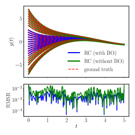
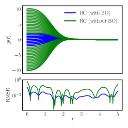
Figure 1: Backpropagation-free training for solving the linear ODEs of Eq. (23) (right) and Eq. (25) (left). Upper graphs outline the RC solutions for different ICs. Lower panels show the RMSR. Blue and green lines represent ICs used and not used in BO.

In both experiments, BO was applied to a bundle of ICs implying that a single set of hyper-parameters is sufficient to construct different RC solutions of the same ODE. In particular, applying BO and using the exact ${\bf W}_{\text{out}}$ of Eq. (20), we get the optimal hyperparameters that yielding the RC solutions shown with blue in Fig. 1. Then, using the same hyperparameters we exactly solve (without BO) for ${\bf W}_{\text{out}}$ to construct RC solutions for different ICs as they are indicated in green in Fig. 1. Moreover, the results shown in Fig. 1 validate the closed-form solution of Eq. (20) verifying that the RC solver is a backpropagation-free unsupervised machine learning method for solving linear first order ODEs.

Nonlinear differential equations, training with gradient descent: It is not possible to derive a closed-form solution for ${\bf W}_{\text{out}}$ for nonlinear ODEs. Nevertheless, RC can solve nonlinear ODEs by training ${\bf W}_{\text{out}}$ using gradient descent (GD). We demonstrate the capacity of RC in solving nonlinear equations by studying Bernoulli type nonlinear equations of the form:

$$a_{1}(t)\dot{y}+a_{0}(t)y+q(t)y^{2}=f(t).$$ (26)

Although it is not possible to derive an exact solution for the optimal ${\bf W}_{\text{out}}$, an approximate closed formula is obtained through a linearization procedure. Then, we use the linearized ${\bf W}_{\text{out}}$ instead of random weights to start the GD. This is a transfer learning approach that drastically accelerates and improves the training (see SM for more details). In the context of linearization approximation any nonlinear term of ${\bf S}{\bf W}_{\text{out}}$ is dropped. This is a valid approximation since ${\bf W}_{\text{out}}\ll 1$ due to the $L_{2}$ regression and ${\bf S}$ varies in the range $[-1,1]$ due to the parametric function of Eq. (21) and the activation functions $\tanh()$ or $\sin()$, which are all bounded within $[-1,1]$. Consequently, we read ${\bf W}_{\text{out}}{\bf S}\ll 1$ and thus, higher orders can be neglected, namely $({\bf W}_{\text{out}}{\bf S})^{\nu}\simeq 0$ for any integer $\nu>1$.

Minimizing the loss function of Eq. (4) for the nonlinear ODE (26) yields

$$\left(A_{1}\dot{Y}+A_{0}Y+QY^{T}Y-F\right)^{T}\frac{\partial}{\partial{\bf W}_{\text{out}}}\left(A_{1}\dot{Y}+A_{0}Y+QY^{T}Y-F\right)+\lambda{\bf W}_{\text{out}}^{T} =0$$

$$\Big{(}{\bf W}_{\text{out}}^{T}D_{\bf H}^{T}+D_{0}^{T}+Q\left(\Psi_{0}^{2}+2\Psi_{0}{\bf W}_{\text{out}}^{T}\right)\Big{)}\Big{(}D_{\bf H}+2Q\left(\Psi_{0}+{\bf S}{\bf W}_{\text{out}}\right)\Big{)}+\lambda{\bf W}_{\text{out}}^{T} =0$$ (27)

$${\bf W}_{\text{out}}^{T}\Big{(}\tilde{D}_{\bf H}^{T}\tilde{D}_{\bf H}+\tilde{2}QD_{0}^{T}{\bf S}+\lambda{\bf 1}\Big{)}+\tilde{D}_{0}^{T}\tilde{D}_{\bf H} =0,$$ (28)

where in Eq. (27) nonlinear terms of ${\bf S}{\bf W}_{\text{out}}$ are dropped. $Q=(q(t_{0}),\dotsc,q(t_{K}))$, and the modified characteristic matrices are defined as:

$$\tilde{D}_{\bf H} =D_{\bf H}+2Q\Psi_{0},$$ (29)

$$\tilde{D}_{0} =D_{0}+Q\Psi_{0}^{2}.$$ (30)

The linear algebraic system of Eq. (28) can be inverted to give the linearized RC weights as:

$${\bf W}_{\text{out}}=-\Big{(}\tilde{D}_{\bf H}^{T}\tilde{D}_{\bf H}+\tilde{2}QD_{0}^{T}{\bf S}+\lambda{\bf 1}\Big{)}^{-1}\tilde{D}_{\bf H}^{T}\tilde{D}_{0}.$$ (31)

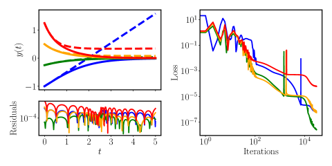
Figure 2: Nonlinear ODE. The upper-left image shows RC solutions obtained by linearized weights (dashed lines) and the solutions obtained after gradient descent optimization (solid lines). The lower-left panel outlines the residuals for each RC solution after applying GD. The graph on the right shows the loss function during the GD iterations. Each color represents a different IC.

We assess the performance of the RC by solving the ODE (26) for $a_{0}=a_{1}=1$, $f=0$, and $q=0.5$. Starting with the linearized ${\bf W}_{\text{out}}$ of Eq. (31), we employ GD to train the parameters. This is efficient since we only optimize a single linear layer. Figure 2 presents the RC solutions (top-left graph) and the associated residuals (bottom-left) for different ICs indicated by different colors. Upper plot: the dashed lines indicate RC predictions obtained by solely applying the linearized ${\bf W}_{\text{out}}$ of Eq. (31), before applying GD; solid lines are the RC predictions after GD. The right side of Fig. 2 outlines the loss function during the GD iterations where each colored loss trace corresponds to the associated colored line in the left plots.

Systems of ordinary differential equations, Hamiltonian systems: In this section, we employ RC to solve systems of ODEs. To apply RC to systems, the network architecture needs to be modified to return multiple outputs $N_{j}$, where $j$ indicates a different output. The number of the $N_{j}$ needs to be the same with the number of the equations in the system. Each $N_{j}$ has a different set of weights ${\bf W}_{\text{out}}^{(j)}$, while all $N_{j}$ share the same hidden states, namely:

$$N_{j}={\bf W}_{\text{out}}^{(j)}\cdot{\tilde{\bf h}}.$$ (32)

Moreover, the loss function (4) includes all the ODEs included in the system. We exploit the RC solver in solving the equations of motion for a nonlinear Hamiltonian system, the nonlinear oscillator. In this system the energy is conserved and thus, we adopt the energy regularization introduced in Ref. [12] that drastically accelerates the training and improves the fidelity of the predicted solutions.

Hamiltonian systems obey the energy conservation law. Specifically, these systems are characterized by a time-invariant hamiltonian function that represents the total energy. The hamiltonian of a nonlinear oscillator with unity mass and frequency is given by:

$$\mathcal{H}(x,p)=\frac{p^{2}}{2}+\frac{x^{2}}{2}+\frac{x^{4}}{4},$$ (33)

and the associated equations of motion read:

$$\dot{x} =p$$ (34)

$$\dot{p} =-x-x^{3}$$ (35)

where $x,~{}p$ are the position and momentum variables [12]. The loss function consists of three parts: $L_{\text{ODE}}$ for the ODEs (34), (35); a hamiltonian penalty $L_{\mathcal{H}}$ that penalizes violations in the energy conservation and is defined by Eq. (33); and a regularization term. Subsequently, the total $L$ is:

$$L =L_{\text{ODE}}+L_{\mathcal{H}}+L_{\text{reg}}$$

$$=\sum_{n=0}^{K}\Big{[}\left(\dot{x}_{n}-p_{n}\right)^{2}+\left(\dot{p}_{n}+x_{n}+x_{n}^{3}\right)^{2}+\left(E-\mathcal{H}(x_{n},p_{n})\right)^{2}\Big{]}+L_{\text{reg}}.$$ (36)

$E=\mathcal{H}(x_{0},p_{0})$ represents the total energy defined by the ICs $x(0)=x_{0}$, $p(0)=p_{0}$. Earlier we choose $L_{2}$ regularization because we derived exact solutions for the ${\bf W}_{\text{out}}$; this was possible with $L_{2}$. For systems of ODEs we do not derive exact ${\bf W}_{\text{out}}$ and thus, we can apply any $L_{\text{reg}}$. We use the elastic net regularization which has been shown to be a dominant generalization of $L_{1}$ and $L_{2}$ (see the SM) [44]. The RC solutions are defined through Eqs. (12) and (32) as:

$$x_{n}=x_{0}+{\bf W}_{\text{out}}^{(x)}\cdot\left(g(t_{n}){\tilde{\bf h}}(t_{n})\right),$$ (37)

$$p_{n}=p_{0}+{\bf W}_{\text{out}}^{(p)}\cdot\left(g(t_{n}){\tilde{\bf h}}(t_{n})\right).$$ (38)

We employ the RC solver from the rcTorch library to solve the Eqs. (34) and (35). Specifically, we minimize Eq. (36) by applying GD and use $g(t)$ of Eq. (21). The results are outlined in Fig. 3. First, we consider a singe set of ICs, $(x_{0},p_{0})=(1.3,1)$, and use the hybrid mode consisting of GD and BO to find the optimal hyper-parameters. This optimization is performed in the time range $t=[0,6\pi]$. Then, using the obtained hyper-parameters we expand the time range to $t=[0,10\pi]$ and generate RC solutions solely using GD. The RC solution for $x$ is presented in the upper left graph, while the lower plot shows the residuals. In both images, the dashed red line indicates the end of the BO. Using the same hyper-parameter set, we apply the RC solver in a range of ICs. The right panel we shows the phase-space diagram ($x-p$ plot) for the IC used in the BO (blue line) and for the ICs where only GD is applied (green lines). In the SM we report the residuals and the loss traces during the GD for all the investigated ICs. Figure 3 is evidence that a single hyper-parameter set can be used to solve an ODE system for different ICs and time ranges.

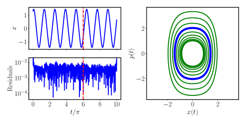
Figure 3: Nonlinear oscillator. Left panel represents a single IC. BO is applied up to red dahsed line. Right graph demonstrate the RC solutions for different ICs not used in BO optimization (green), while blue line is associated to the solution shown in the left plot.

5 Conclusion

Recently, NN differential equation solvers have attracted a lot of interest. These solvers present some crucial advantages over traditional integrators such as they provide analytical and differentiable solutions that can be inverted, suffer less from the "curse of dimensionality", and learn general solutions. While many methods and scientific libraries for NN solvers have been reported an RNN solver is still missing from the literature.

Novelty: We presented a novel RNN ODE solver in the context of an unsupervised RC and assessed the performance of the RC solver by solving linear and nonlinear ODEs. We showed that a closed-form solution for the RC weights is possible for solving linear ODEs with explicit time dependence, leading to a backpropagation-free optimization method. For nonlinear system, we applied GD which is very efficient since in the RC architecture we train only a linear output layer. For the hyper-parameter optimization, we employed BO integrated with GD. We found that a single set of hyper-parameters can be shared for solving ODEs for different initial conditions and time intervals.

Limitations: For BO we used TURBO-1, however, dominant methods such as TURBO-m have been shown to be more robust and get stuck less often in local minima. The efficacy of the proposed RC solver has not been corroborated for very demanding ODEs due to the limited capacity in finding optimal hyperparameters. Although we derived a closed-form solution for a single linear ODE, such a closed formula has not been derived for linear systems of ODEs. Hence, GD is required for solving systems. The proposed RC architecture takes an input $t$ restricting the RC to solve only ODEs. With more variables as inputs, the RC will be able to solve partial differential equations.Currently a uniformly spaced input $t$ has been used, so the efficacy of RC in solving stiff ODEs is not yet determined. A thorough investigation of the optimal reservoir dynamics has not been performed in this study. In this work, we demonstrated that unsupervised RC can solve ODEs by solving a few specific problems using the rcTorch library. Future updates of rcTorch will remove the weakness discussed above, significantly expanding the potential applications of the library. A more general and more powerful rcTorch version is slated to be released in the coming months.

Training an RC is extremely fast (see SM for runtime details and coding demonstrations). Although more investigation is warranted, RC has the potential to make NN solvers dramatically faster and even potentially competitive with integrators. Furthermore, RC has widely been adopted to form neuromorphic devices. Since a single set of hyper-parameters can be used to solve a system of ODEs for different ranges of ICs and time ranges, a physical reservoir can be designed to respect these hyper-parameters. Then a readout output layer will be efficiently trained to solve a system of ODEs for different ICs and times. Subsequently, the proposed machine learning method can be potentially implemented to form a neuromorphic computing device for solving ODEs.

6 Broader Impact

Solving differential equations is substantial in every scientific field including engineering, applied physics, quantum chemistry, finance, and biology. Solving these equations can be extremely demanding and frequently prohibitive due to the limitations of existing numerical methods. Subsequently, new technologies and more efficient methods for solving differential equations are crucial to accelerate progress in scientific research. In this work, we introduced a general framework for solving differential equations with recurrent neural networks. We demonstrate the method by solving systems of ordinary differential equations. Yet, this method can be expanded to systems of partial differential equations as well as eigenvalue problems. Moreover, we suggest a computationally efficient method to calculate time derivatives of the outputs of recurrent networks, making possible the development of recurrent data-driven physics-informed neural networks.

Societal and Environmental Impact: Solving differential equations with RC may have negative social impacts depending on what the user employs them for, but they are not immediately obvious and are likely indirect. As far as the environment is concerned, Bayesian optimization can be computationally expensive, but it is not expensive enough to warrant concerns about environmental impacts when compared to heavier models like transformers, feed forward networks or RNNs such as LSTMs. There is an upfront cost with RC, but even after taking this into consideration, our models are likely faster, more efficient, and much less energy intensive (having a smaller carbon footprint) than comparable feed forward neural network differential equation solvers. Moreover, the proposed method can potentially be used to build neuromorphic devices, drastically accelerating computations with extremely low energy consumption.

Checklist

1. For all authors…

   1. Do the main claims made in the abstract and introduction accurately reflect the paper’s contributions and scope? [Yes]

   2. Did you describe the limitations of your work? [Yes] . See section: Conclusion.

   3. Did you discuss any potential negative societal impacts of your work? [Yes] . See section: Broader Impact.

   4. Have you read the ethics review guidelines and ensured that your paper conforms to them? [Yes] .

2. If you are including theoretical results…

   1. Did you state the full set of assumptions of all theoretical results? [Yes] . Sections 3 and 4 have complete discussions.

   2. Did you include complete proofs of all theoretical results? [Yes] . Section 3 and 4 contain all the proofs.

3. If you ran experiments…

   1. Did you include the code, data, and instructions needed to reproduce the main experimental results (either in the supplemental material or as a URL)? [Yes] . Details can be found in the supplementary material (SM). We also provide the URL for a github public repository that contains the library and notebooks used in this study.

   2. Did you specify all the training details (e.g., data splits, hyperparameters, how they were chosen)? [Yes] . They are stated in section 4 and more details can be found in the SM.

   3. Did you report error bars (e.g., with respect to the random seed after running experiments multiple times)? [Yes] . In section 4 and in the SM.

   4. Did you include the total amount of compute and the type of resources used (e.g., type of GPUs, internal cluster, or cloud provider)? [Yes] . All the details are reported in the SM.

4. If you are using existing assets (e.g., code, data, models) or curating/releasing new assets…

   1. If your work uses existing assets, did you cite the creators? [Yes] .

   2. Did you mention the license of the assets? [Yes] .

   3. Did you include any new assets either in the supplemental material or as a URL? [Yes] . Yes, a new asset for the library used in this study is included.

   4. Did you discuss whether and how consent was obtained from people whose data you’re using/curating? [N/A] . There was no need for consent.

   5. Did you discuss whether the data you are using/curating contains personally identifiable information or offensive content? [N/A] . In this neural network method we do not use data for the training.

5. If you used crowdsourcing or conducted research with human subjects…

   1. Did you include the full text of instructions given to participants and screenshots, if applicable? [N/A] . We did not use crowdsourcing or conducted research with human subjects.

   2. Did you describe any potential participant risks, with links to Institutional Review Board (IRB) approvals, if applicable? [N/A] . We did not use crowdsourcing or conducted research with human subjects.

   3. Did you include the estimated hourly wage paid to participants and the total amount spent on participant compensation? [N/A] . We did not use crowdsourcing or conducted research with human subjects.

References

- [1] Lu Lu et al. “Learning nonlinear operators via DeepONet based on the universal approximation theorem of operators involving nonlinear partial differential equations” In Nature machine intelligence 3, 2021, pp. 218–229 DOI: https://doi.org/10.1038/s42256-021-00302-5
- [2] Samuel H. Rudy, Steven L. Brunton, Joshua L. Proctor and J. Nathan Kutz “Data-driven discovery of partial differential equations” In Science Advances 3.4, 2017 DOI: 10.1126/sciadv.1602614
- [3] J. Nathan Kutz, Samuel H. Rudy, Alessandro Alla and Steven L. Brunton “Data-Driven discovery of governing physical laws and their parametric dependencies in engineering, physics and biology” In 2017 IEEE 7th International Workshop on Computational Advances in Multi-Sensor Adaptive Processing (CAMSAP), 2017, pp. 1–5 DOI: 10.1109/CAMSAP.2017.8313100
- [4] Yohai Bar-Sinai, Stephan Hoyer, Jason Hickey and Michael P. Brenner “Learning data-driven discretizations for partial differential equations” In Proceedings of the National Academy of Sciences of the United States of America 116.31, 2019, pp. 15344–15349 DOI: 10.1073/pnas.1814058116
- [5] Sam Greydanus, Misko Dzamba and Jason Yosinski “Hamiltonian Neural Networks” In Advances in Neural Information Processing Systems 32 Curran Associates, Inc., 2019, pp. 15379–15389 URL: http://papers.nips.cc/paper/9672-hamiltonian-neural-networks.pdf
- [6] Tom Bertalan, Felix Dietrich, Igor Mezic and Ioannis G. Kevrekidis “On learning Hamiltonian systems from data” In Chaos: An Interdisciplinary Journal of Nonlinear Science 29.12, 2019, pp. 121107 DOI: 10.1063/1.5128231
- [7] Anshul Choudhary et al. “Physics-enhanced neural networks learn order and chaos” In Phys. Rev. E 101 American Physical Society, 2020, pp. 062207 DOI: 10.1103/PhysRevE.101.062207
- [8] Yuyao Chen, Lu Lu, George Em Karniadakis and Luca Dal Negro “Physics-informed neural networks for inverse problems in nano-optics and metamaterials” In Opt. Express 28.8 OSA, 2020, pp. 11618–11633 DOI: 10.1364/OE.384875
- [9] Isaac E. Lagaris, Aristidis Likas and Dimitrios I. Fotiadis “Artificial neural networks for solving ordinary and partial differential equations” In IEEE transactions on neural networks 9, 1998, pp. 987–1000 DOI: 10.1109/72.712178
- [10] Pola Lydia Lagari, Lefteri H. Tsoukalas, Salar Safarkhani and Isaac E. Lagaris “Systematic Construction of Neural Forms for Solving Partial Differential Equations Inside Rectangular Domains, Subject to Initial, Boundary and Interface Conditions” In International Journal on Artificial Intelligence Tools 29, 2020, pp. 2050009 DOI: 10.1142/S0218213020500098
- [11] Cedric Flamant, Pavlos Protopapas and David Sondak “Solving Differential Equations Using Neural Network Solution Bundles”, 2020 arXiv:2006.14372 [cs.LG]
- [12] Marios Mattheakis, David Sondak, Akshunna S. Dogra and Pavlos Protopapas “Hamiltonian Neural Networks for solving differential equations” In arXiv:2001.11107 [physics], 2020 URL: http://arxiv.org/abs/2001.11107
- [13] Jiequn Han, Arnulf Jentzen and E Weinan “Solving high-dimensional partial differential equations using deep learning” In Proceedings of the National Academy of Sciences of the United States of America 115 34, 2017, pp. 8505–8510 DOI: 10.1073/pnas.1718942115
- [14] Justin A. Sirignano and Konstantinos Spiliopoulos “DGM: A deep learning algorithm for solving partial differential equations” In Journal of Computational Physics 375, 2018, pp. 1339–1364 DOI: 10.1016/j.jcp.2018.08.029
- [15] Feiyu Chen et al. “NeuroDiffEq: A Python package for solving differential equations with neural networks” In Journal of Open Source Software 5.46 The Open Journal, 2020, pp. 1931 DOI: 10.21105/joss.01931
- [16] Henry Jin, Marios Mattheakis and Pavlos Protopapas “Unsupervised Neural Networks for Quantum Eigenvalue Problems” In 2020 NeurIPS Workshop on Machine Learning and the Physical Sciences NeurIPS, 2020 URL: https://ml4physicalsciences.github.io/2020/files/NeurIPS_ML4PS_2020_16.pdf
- [17] Alessandro Paticchio et al. “Semi-supervised Neural Networks solve an inverse problem for modeling Covid-19 spread” In 2020 NeurIPS Workshop on Machine Learning and the Physical Sciences NeurIPS, 2020 URL: https://ml4physicalsciences.github.io/2020/files/NeurIPS_ML4PS_2020_29.pdf
- [18] P. Grohs, F. Hornung, A. Jentzen and P. Von Wurstemberger “A proof that artificial neural networks overcome the curse of dimensionality in the numerical approximation of Black-Scholes partial differential equations” In arXiv:1809.02362 [math.NA], 2018 URL: https://arxiv.org/abs/1809.02362
- [19] M. Raissi, P. Perdikaris and G.E. Karniadakis “Physics-informed neural networks: A deep learning framework for solving forward and inverse problems involving nonlinear partial differential equations” In Journal of Computational Physics 378, 2019, pp. 686–707 DOI: https://doi.org/10.1016/j.jcp.2018.10.045
- [20] Herbert Jaeger and Harald Haas “Harnessing Nonlinearity: Predicting Chaotic Systems and Saving Energy in Wireless Communication” In Science 304.5667 American Association for the Advancement of Science, 2004, pp. 78–80 DOI: 10.1126/science.1091277
- [21] Zhixin Lu et al. “Reservoir observers: Model-free inference of unmeasured variables in chaotic systems” In Chaos 27.4, 2017 DOI: 10.1063/1.4979665
- [22] George Neofotistos et al. “Machine Learning With Observers Predicts Complex Spatiotemporal Behavior” In Frontiers in Physics 7, 2019, pp. 24 DOI: 10.3389/fphy.2019.00024
- [23] Jaideep Pathak et al. “Model-Free Prediction of Large Spatiotemporally Chaotic Systems from Data: A Reservoir Computing Approach” In Phys. Rev. Lett. 120 American Physical Society, 2018, pp. 024102 DOI: 10.1103/PhysRevLett.120.024102
- [24] Jonathan Dong, Ruben Ohana, Mushegh Rafayelyan and Florent Krzakala “Reservoir Computing meets Recurrent Kernels and Structured Transforms” In Advances in Neural Information Processing Systems 33 Curran Associates, Inc., 2020, pp. 16785–16796 URL: https://proceedings.neurips.cc/paper/2020/file/c348616cd8a86ee661c7c98800678fad-Paper.pdf
- [25] Sandra Nestler et al. “Unfolding recurrence by Green’s functions for optimized reservoir computing” In Advances in Neural Information Processing Systems 33 Curran Associates, Inc., 2020, pp. 17380–17390 URL: https://proceedings.neurips.cc/paper/2020/file/c94a589bdd47870b1d74b258d1ce3b33-Paper.pdf
- [26] Anteo Smerieri et al. “Analog readout for optical reservoir computers” In Advances in Neural Information Processing Systems 25 Curran Associates, Inc., 2012 URL: https://proceedings.neurips.cc/paper/2012/file/250cf8b51c773f3f8dc8b4be867a9a02-Paper.pdf
- [27] Andrew Katumba et al. “Low-loss photonic reservoir computing with multimode photonic integrated circuits” In SCIENTIFIC REPORTS 8.1 Springer Nature, 2018, pp. 2653:1–2653:10 DOI: 10.1038/s41598-018-21011-x
- [28] G. Tanaka et al. “Recent Advances in Physical Reservoir Computing: A Review” In Neural networks : the official journal of the International Neural Network Society 115, 2019, pp. 100–123 DOI: /10.1016/j.neunet.2019.03.005
- [29] Satoshi Sunada and Atsushi Uchida “Photonic reservoir computing based on nonlinear wave dynamics at microscale” In SCIENTIFIC REPORTS 9.1 Springer Nature, 2019, pp. 19078:1–19078:10 DOI: 10.1038/s41598-019-55247-y
- [30] Laurent Larger et al. “High-Speed Photonic Reservoir Computing Using a Time-Delay-Based Architecture: Million Words per Second Classification” In Phys. Rev. X 7 American Physical Society, 2017, pp. 011015 DOI: 10.1103/PhysRevX.7.011015
- [31] Giulia Marcucci, Davide Pierangeli and Claudio Conti “Theory of Neuromorphic Computing by Waves: Machine Learning by Rogue Waves, Dispersive Shocks, and Solitons” In Phys. Rev. Lett. 125 American Physical Society, 2020, pp. 093901 DOI: 10.1103/PhysRevLett.125.093901
- [32] Huong Ha et al. “Bayesian Optimization with Unknown Search Space”, 2019 arXiv:1910.13092 [stat.ML]
- [33] David Eriksson et al. “Scalable Global Optimization via Local Bayesian Optimization”, 2020 arXiv:1910.01739 [cs.LG]
- [34] Jacob Reinier Maat, Nikos Gianniotis and Pavlos Protopapas “Efficient Optimization of Echo State Networks for Time Series Datasets” In 2018 International Joint Conference on Neural Networks (IJCNN), 2018, pp. 1–7 DOI: 10.1109/IJCNN.2018.8489094
- [35] Zhongxiang Dai, Kian Hsiang Low and Patrick Jaillet “Federated Bayesian Optimization via Thompson Sampling”, 2020 arXiv:2010.10154 [cs.LG]
- [36] Maximilian Balandat et al. “BoTorch: A Framework for Efficient Monte-Carlo Bayesian Optimization” In Advances in Neural Information Processing Systems 33 Curran Associates, Inc., 2020, pp. 21524–21538 URL: https://proceedings.neurips.cc/paper/2020/file/f5b1b89d98b7286673128a5fb112cb9a-Paper.pdf
- [37] Lu Lu, Xuhui Meng, Zhiping Mao and George E. Karniadakis “A deep learning library for solving differential equations” In SIAM Review 63, 2021, pp. 208–228 DOI: 10.1137/19M1274067
- [38] Oliver Hennigh et al. “NVIDIA SimNet: an AI-accelerated multi-physics simulation framework” In arXiv:2012.07938 [physics.flu-dyn], 2020 URL: https://arxiv.org/abs/2012.07938
- [39] George Em Karniadakis et al. “Physics-informed machine learning” In Nature Review Physics, 2021 DOI: https://doi.org/10.1038/s42254-021-00314-5
- [40] Kurt Hornik “Approximation capabilities of multilayer feedforward networks” In Neural Networks 4, 1991, pp. 251–257 DOI: 10.1016/0893-6080(91)90009-T
- [41] Bo Chang et al. “Reversible Architectures for Arbitrarily Deep Residual Neural Networks”, 2018 URL: https://aaai.org/ocs/index.php/AAAI/AAAI18/paper/view/16517
- [42] Ricky T. Q. Chen, Yulia Rubanova, Jesse Bettencourt and David K Duvenaud “Neural Ordinary Differential Equations” In Advances in Neural Information Processing Systems 31, 2018 URL: https://proceedings.neurips.cc/paper/2018/file/69386f6bb1dfed68692a24c8686939b9-Paper.pdf
- [43] Michael Poli et al. “Hypersolvers: Toward Fast Continuous-Depth Models” In Advances in Neural Information Processing Systems 33 Curran Associates, Inc., 2020, pp. 21105–21117 URL: https://proceedings.neurips.cc/paper/2020/file/f1686b4badcf28d33ed632036c7ab0b8-Paper.pdf
- [44] Hui Zou and Trevor Hastie “Regularization and variable selection via the Elastic Net” In Journal of the Royal Statistical Society, Series B 67, 2005, pp. 301–320