Encoding Scheme for Infinite Set of Symbols:
the Percolation Process on Infinite Perfect Binary Trees

Abstract

It is shown here that the percolation cluster that emerges from the percolation process on infinite perfect binary trees, is genuinely an encoding scheme for an infinite set of symbols. The average codeword length and the entropy of such an encoding scheme are still finite as long as the percolation density $p$ is between $1/2\leq p<\sqrt[3]{1/4}$.

Keywords Binary Tree $\cdot$ Efficient Encoding  $\cdot$ Entropy  $\cdot$ Huffman Encoding Scheme  $\cdot$ Percolation Process  $\cdot$ Bienaymé-Galton-Watson Process

1 Introduction

Binary trees are perennial and indispensable part of information and coding theory in computer science. They are used for storage file systems and databases [1, 2]. For instance, the Btrfs (pronounced as B-Tree Filesystem) is a filesystem utilising the Balanced Tree structure to store large data [3]. In databases, indexing in many widely used database software such as PostgreSQL and Oracle SQL use B-tree indexing (see their respective documentations and also refer to [4] for recent methods and technologies). In a different area -data compression- the foundation of much popular data compression software such as .arc, .pk(X)zip, gzip, .bzip and the famous .zip is based on the Huffman encoding scheme [5].

In real-life cases, the source of the information is represented by a finite set of symbols (also called alphabets). In these situations, the Huffman encoding scheme ensures via an encoding procedure that the length of the codewords associated to each symbol yields an average codeword length which is the smallest given the frequency of the appearance of each symbol in the source [5]. Yet, one can get audacious and think of a situation where the set of symbols is countably infinite. Although, this would not happen in day to day problems, one can ask whether there exists a physical process that genuinely encodes the information in a manner that yields a finite average codeword length. For instance, one can consider a physical system with a set of discrete energy levels that are countably infinite. If one attempts to label these discrete levels with a set of codewords, what are the criteria such that these energy levels are expressed in these codewords and still on average the codeword length is finite.

In this article, it is demonstrated that the Bienaymé-Galton-Watson process with maximum two offspring [6, 7], is a process that itself generates the symbols and encodes them simultaneously in such a manner that the state of the system described by these symbols can be expressed with an infinite set of codewords that yields a finite average codeword length. The Bienaymé-Galton-Watson process with maximum two offspring has an equivalent representation, namely the percolation process on infinite perfect binary trees. Applications of the percolation process are far-reaching in many areas, ranging from soft materials such as polymers [8, 9] to brittle and rigid materials such as rock [10]. It has been used to model the financial markets [11, 12] or division of labour markets [13] or to understand the dynamics of a protein in lipid membranes [14]. Yet with many of these applications, little has been said on the application of the percolation process from the perspective of information theory and coding theory [15]. It is demonstrated here that the percolation cluster that emerges at the critical percolation density $p_{c}$ has undeniable similarity to the well-known Huffman encoding scheme. This establishes a direct connection between the Bienaymé-Galton-Watson process, the percolation process and the Huffman encoding scheme.

The structure of this article is such that it first gives a gentle introduction to the Bienaymé-Galton-Watson process. Then it is shown that it is equivalent to the percolation process on perfect binary trees if the number of the offspring is limited to maximum of two descendants. The section afterwards is dedicated to the derivation of the generalised probability generating function for the Bienaymé-Galton-Watson process. With the generalised probability function in hand, one then can investigate the number of nodes and leaves of the percolation cluster at different generations. The last section concludes the results and provides the reader with comparisons between the analytical and the simulation results.

2 Bienaymé-Galton-Watson Process and Percolation Process on Perfect Binary Trees

The Bienaymé-Galton-Watson process is a branching process $\{\mathcal{N}_{n}\}_{n\in\mathbb{N}}$ where $n\in\mathbb{N}$ is called the generation and $\mathcal{N}_{n}$ the population of the $n^{th}$ generation. Each member of a generation has the possibility to have offspring in the next generation according to a specific probability distribution. The central question here is to know the number of the population at the $(n+1)^{th}$ generation given the number of the population at the $n^{th}$ generation.

In the most simplest form, it is assumed that the number of offspring each member of a generation has is independent of the other members of that generation or any other generations before. If the number of offspring the $i^{th}$ member of the $n^{th}$ generation has is denoted by $X_{n}^{i}\in\mathbb{N}$, then the assumption made earlier implies that $X_{n}^{i}$’s are i.i.d random variables according to a given fixed probability distribution. Therefore,

$$\mathcal{N}_{n+1}=\sum_{i=1}^{\mathcal{N}_{n}}X_{n}^{i}.$$ (1)

It follows immediately that the transition probability function for the process is as follows [16]

$$P\big{(}\mathcal{N}_{n}=i\,|\,\mathcal{N}_{n-1}=j\big{)}=\begin{cases}p_{i}^{*j},&\text{if}\quad i\geq 1,\,j\geq 0\\ \delta_{0i},&\text{if}\quad i=0,\,j\geq 0\end{cases},$$ (2)

where $p_{i}^{*j}$ is understood as the $j$-fold probability convolution. Note that this probability transition function implies that the process is a Markov chain.

There is a kin relation between the Bienaymé-Galton-Watson process and the percolation process on trees. Since the ultimate goal of this article is about information encoding, henceforth only the binary trees are assumed here. Specifically, consider infinite perfect binary trees with the root $\emptyset$ at the top. The percolation process on such trees is the process of assigning to each edge independent of any other edges the state of being open with probability $p$and the state of being closed with probability $q=1-p$. The probability $p$ is also known as the percolation density. The nodes in the immediate vicinity of the root belong to the first generation and are the offspring of the root. The nodes that are in the immediate vicinity of the nodes in the first generation belong to the second generation and so on. A realisation of such a process on a perfect binary tree up to the third generation is shown in Fig. 1.

Figure 1: A perfect binary tree with $n=3$. The percolation process on this tree left behind a set of open edges (solid lines) along with closed edges (dashed lines) with probability $p$ and $q$ respectively.

An open path between a node in the $n^{th}$ generation and a node in the $m^{th}$ generation is a sequence of open edges that starts at the former node and ends at the latter. Consequently, two nodes are said to be connected if there is an open path between them. A set of nodes that are connected form an open cluster. The size of an open cluster is simply the number of nodes it has. A node is also said to be a leaf if it does not have any offspring.

When $p=1$, a single perfect tree emerges and all the nodes belong to one unique open cluster. On the other hand, when $q=1$, nodes are trivial trees. In this case, one has a forest in which the nodes are the trivial trees in this forest. In Bienaymé-Galton-Watson process if the probabilities of having offspring more than two are zero, then every open cluster of the percolation process is a realisation of a Bienaymé-Galton-Watson process that commences at a node which is not the offspring of any other node.

The interesting fact here though is the emergence of an infinite open cluster that includes the root when $p$ reaches a critical value called $p_{c}$ when for the first time an open cluster called the percolation cluster emerges that is infinite in size when $n\rightarrow\infty$. This corresponds to the critical Bienaymé-Galton-Watson process when it thrives ad infinitum. It is possible to investigate the distribution of the nodes and leaves at $p_{c}$ (also for any other $p$) using the known tool of probability generating functions [17, 18] discussed in the following subsection.

2.1 Probability generating function of the Bienaymé-Galton-Watson process

The probability generating function for the Bienaymé-Galton-Watson process over the states $\mathbb{N}=\{0,1,2,\cdots\}$ and the associated probabilities $\{p_{k}\}_{k\in\mathbb{N}}$ is defined by

$$f(\xi)=\sum_{k=0}^{\infty}p_{k}\xi^{k},\quad|\xi|\leq 1,$$ (3)

where the dummy index $k$ counts the number of offspring and $p_{k}$ is the probability of having $k$ offspring. Note that in the case of binary trees, $p_{k}=0$ for all $k>2$. Hence, the upper bound of the sum is identically 2. Nonetheless, the results derived henceforth in this section are not limited to this constraint. The iterates of the probability generating function Eq. (3) are given by

$$f_{0}(\xi)=\xi,\quad f_{1}(\xi)=f(\xi),\quad f_{n}(\xi)=f[f_{n-1}(\xi)].$$

It is not difficult to establish the following using Eq. (2)

$$\sum_{k}P(\mathcal{N}_{n}=k\,|\,\mathcal{N}_{n-1}=1)\xi^{k}=\sum_{k}p_{k}\xi^{k}=f(\xi),$$ (4a)

$$\sum_{k}P(\mathcal{N}_{n}=k\,|\,\mathcal{N}_{n-1}=i)\xi^{k}=[f(\xi)]^{i}.$$ (4b)

The most central identity concerning the probability generating function defined in Eq. (3) and the probability transition function given by Eq. (2) is the one that establishes a relation between the $n^{th}$ iterate of the probability generating function $f_{n}(\xi)$ and the probability generating function associated with the $n^{th}$ step of the probability transition function, denoted by $f_{(n)}(\xi)$. Due to Chapman-Kolmogorov equation  for Markov chains observe that

$$f_{(n)}(\xi) =\sum_{k}P(\mathcal{N}_{n}=k\,|\,\mathcal{N}_{0}=1)\xi^{k}=\sum_{k}\sum_{s}P(\mathcal{N}_{n-1}=s\,|\,\mathcal{N}_{0}=1)P(\mathcal{N}_{n}=k\,|\,\mathcal{N}_{n-1}=s)\xi^{k}$$

$$=\sum_{s}P(\mathcal{N}_{n-1}=s\,|\,\mathcal{N}_{0}=1)\sum_{k}P(\mathcal{N}_{n}=k\,|\,\mathcal{N}_{n-1}=s)\xi^{k}$$

$$=\sum_{s}P(\mathcal{N}_{n-1}=s\,|\,\mathcal{N}_{0}=1)[f(\xi)]^{s}=f_{(n-1)}[f(\xi)]=\underbrace{f[\cdots[f(\xi)]]}_{n\text{times}}=f_{n}(\xi)$$ (5)

The identity above is crucial to deduce moments and properties of the Bianaymé-Galton-Watson process. In this regard, first note that the mean and the variance of the population in the first generation can be calculated via the probability generating function $f(\xi)$.

$$\frac{d}{d\xi}f(\xi)\Big{|}_{\xi=1}=\sum_{k=0}^{2}kp_{k}=\mathbb{E}[\mathcal{N}_{1}]:=\mu,$$ (6a)

$$\frac{d^{2}}{d\xi^{2}}f(\xi)\Big{|}_{\xi=1}=\sum_{k=0}^{2}k(k-1)p_{k}=\mathrm{Var}[\mathcal{N}_{1}]-\mu+\mu^{2}.$$ (6b)

Moreover

$$\mathbb{E}[\mathcal{N}_{n}] =\frac{d}{d\xi}f_{(n)}(\xi)\Big{|}_{\xi=1}=\frac{d}{d\xi}f_{n}(\xi)\Big{|}_{\xi=1}=\frac{d}{d\xi}f[f_{n-1}(\xi)]\Big{|}_{\xi=1}$$

$$=f^{\prime}[f_{n-1}(\xi)]f^{\prime}_{n-1}(\xi)\Big{|}_{\xi=1}=f^{\prime}(1)f^{\prime}_{n-1}(1)=[f^{\prime}(1)]^{n}=\mu^{n},$$ (7)

where the prime in $f^{\prime}(.)$ stands on the derivative with respect to the argument. In the last step, one recursively invokes the same identity for $f^{\prime}_{n-1}(\xi)$ and arrives at $\mu^{n}$. Follow the same procedure and deduce that

$$\mathrm{Var}[\mathcal{N}_{n}]-\mu^{n}+\mu^{2n} =\frac{d^{2}}{d\xi^{2}}f_{(n)}(\xi)\Big{|}_{\xi=1}=\frac{d^{2}}{d\xi^{2}}f_{n}(\xi)\Big{|}_{\xi=1}=\frac{d^{2}}{d\xi^{2}}f[f_{n-1}(\xi)]$$

$$=f^{\prime\prime}[f_{n-1}(\xi)](f^{\prime}_{n-1}(\xi))^{2}\Big{|}_{\xi=1}+f^{\prime}[f_{n-1}(\xi)]f^{\prime\prime}_{n-1}(\xi)\Big{|}_{\xi=1}$$

$$=f^{\prime\prime}(1)\mu^{2n-2}+\mu f^{\prime\prime}_{n-1}(1)=f^{\prime\prime}(1)\mu^{2n-2}\sum_{i=0}^{n-1}\mu^{-i}.$$ (8)

The last line in the equation above is due to applying recursively the identity $f^{\prime\prime}_{n}(1)=f^{\prime\prime}(1)\mu^{2n-2}+\mu f^{\prime\prime}_{n-1}(1)$. Depending on the value of $\mu$ and by substituting $f^{\prime\prime}(1)$ with Eq. (6b) the variance obeys the following expressions

$$\mathrm{Var}[\mathcal{N}_{n}]=\begin{cases}\mathrm{Var}[\mathcal{N}_{1}]\mu^{n}\left(\frac{\mu^{n}-1}{\mu^{2}-\mu}\right),&\text{if}\quad\mu\neq 1\\ n\mathrm{Var}[\mathcal{N}_{1}],&\text{if}\quad\mu=1\end{cases}.$$ (9)

So far, the discussion was focused on the statistical properties of $\mathcal{N}_{n}$ . In the picture of the percolation process on infinite perfect binary trees $\mathcal{N}_{n}$’s correspond to the number of nodes at different generations. Yet, the number of those nodes without any offspring (called leaves) is of utmost importance in the upcoming section. The number of leaves at generation $n$ is a random variable $\mathcal{L}_{n}$ and it is formally given by the following sum.

$$\mathcal{L}_{n}=\sum_{i=1}^{\mathcal{N}_{n}}\mathds{1}_{L}(i),$$

where $\mathds{1}_{L}(i)$ is an indicator function such that $\mathds{1}_{L}(i)=1$ if $i$ belongs to the set of leaves $\overline{L}\subset\{\mathcal{N}_{n}\}$ and is zero otherwise. The notation $\{\mathcal{N}_{n}\}$ indicates the set of the population at the $n^{th}$ generation. The probability transition function for $\mathcal{L}_{n}$ is read as

$$\mathrm{Pr}(\mathcal{L}_{n}=i\,|\,,\mathcal{N}_{n}=j\wedge\mathcal{N}_{n-1}=k)=P(\mathcal{L}_{n}=i\,|\,\mathcal{N}_{n}=j)P(\mathcal{N}_{n}=j\,|\,\mathcal{N}_{n-1}=k).$$ (10)

This implies that the probability of observing $i$ leaves at generation $n$ is the joint probability of having $j$ nodes at the same generation given that the number of nodes in the previous generation is $k$, and from those $j$ nodes $i$ of them are leaves i.e.

$$P(\mathcal{L}_{n}=i\,|\,\mathcal{N}_{n}=j\wedge\mathcal{N}_{n_{1}}=1)=$$

$$P(\mathcal{L}_{n}=i\,|\,\mathcal{N}_{n}=j)P(\mathcal{N}_{n}=j\,|\,\mathcal{N}_{n-1}=1)=\binom{j}{i}u_{1}^{i}u_{0}^{j-i}p_{j}.$$

Here $u_{1}$ is the probability of being a leaf whilst $u_{0}$ is the probability of not being a leaf. The notation $\binom{j}{i}$ stands on choosing $i$ elements from $j$ elements. Multiply both sides by $\xi^{j}\zeta^{i}$ and sum over $i$ and $j$ and arrive at the following.

$$\sum_{i,j}P(\mathcal{L}_{n}=i\,|\,\mathcal{N}_{n}=j)P(\mathcal{N}_{n}=j\,|\,\mathcal{N}_{n-1}=1)=$$

$$\sum_{j}p_{j}\xi^{j}\sum_{i}\binom{j}{i}u_{1}^{i}u_{0}^{j-i}\zeta^{i}=\sum_{j}p_{j}[\xi(u_{1}\zeta+u_{0})]^{j}=f\big{(}\xi g(\zeta)\big{)},$$ (11)

where $g(\zeta)=(u_{1}\zeta+u_{0})$ is the probability generating function of the state of a single node being a leaf or not and $f\big{(}\xi g(\zeta\big{)}$ is the generalised probability generating function that includes the information of both the number of nodes and leaves at a given generation $n$.

The generalised probability generating function satisfies the same properties that $f(\xi)$ exhibits. For instance

$$f_{(n)}\big{(}\xi g(\zeta)\big{)} =\sum_{i,j}P(\mathcal{L}_{n}=i\,|\,\mathcal{N}_{n}=j\wedge\mathcal{N}_{0}=1)\xi^{j}\zeta^{i}$$

$$=\sum_{i,j}P(\mathcal{L}_{n}=i\,|\,\mathcal{N}_{n}=j)P(\mathcal{N}_{n}=j\,|\,\mathcal{N}_{0}=1)\xi^{j}\zeta^{i}$$

$$=\sum_{i,j}P(\mathcal{L}_{n}=i\,|\,\mathcal{N}_{n}=j)\sum_{k}P(\mathcal{N}_{n}=i\,|\,\mathcal{N}_{n-1}=k)P(\mathcal{N}_{n-1}=k\,|\,\mathcal{N}_{0}=1)\xi^{j}\zeta^{i}$$

$$=\sum_{k}P(\mathcal{N}_{n-1}=k\,|\,\mathcal{N}_{0}=1)\left[f\big{(}\xi g(\zeta)\big{)}\right]^{k}=f_{(n-1)}\left[f\big{(}\xi g(\zeta)\big{)}\right]=f_{n}\big{(}\xi g(\zeta)\big{)},$$ (12)

where the last term is followed by induction. The average number of leaves at a given generation $n$ is achieved by taking the first order partial derivative of $f_{(n)}\big{(}\xi g(\zeta)\big{)}$ with respect to $\zeta$

$$\mathbb{E}[\mathcal{L}_{n}] =\frac{\partial}{\partial\zeta}f_{(n)}\big{(}\xi g(\zeta)\big{)}\Big{|}_{\xi=\zeta=1}=\frac{\partial}{\partial\zeta}f_{n}\big{(}\xi g(\zeta)\big{)}\Big{|}_{\xi=\zeta=1}=\frac{\partial}{\partial\zeta}f[f_{n-1}\big{(}\xi g(\zeta)\big{)}]\Big{|}_{\xi=\zeta=1}$$

$$=f^{\prime}\left[f_{n-1}\big{(}\xi g(\zeta)\big{)}\right]f^{\prime}_{n-1}\big{(}\xi g(\zeta)\big{)}\xi g^{\prime}(\zeta)\Big{|}_{\xi=\zeta=1}$$

$$=u_{1}f^{\prime}(1)f^{\prime}_{n-1}(1)=u_{1}[f^{\prime}(1)]^{n}=u_{1}\mathbb{E}[\mathcal{N}_{n}]=u_{1}\mu^{n},$$ (13)

where in the last line the identity that $f^{\prime}_{n}(1)=[f^{\prime}(1)]^{n}$ derived in Eq. (7) is used. In a similar fashion used in Eq. (8) the variance of $\mathcal{L}_{n}$ is deduced to be

$$\mathrm{Var}[\mathcal{L}_{n}]=u_{1}^{2}\mathrm{Var}[\mathcal{N}_{n}].$$ (14)

2.2 The percolation process on perfect binary trees and the statistical properties of $\mathcal{N}_{n}$ and $\mathcal{L}_{n}$

As previously mentioned, percolation process is equivalent to the Bienaymé -Galton-Watson process discussed earlier. If one limits the number of offspring of each node only to the set $\{0,1,2\}$, then one deals with the percolation process on perfect binary trees. The fact that a node does not have any offspring corresponds to the situation where the edges coming out of that very node are both closed which corresponds to the probability $q^{2}$. Likewise, the possibility of having only one offspring corresponds to the situation where one edge is closed and the other one is open which implies the probability $2pq$ and having exactly two offspring indicates that both edges are open and the probability associated to this event is $p^{2}$. Hence one identifies the probabilities $p_{0},p_{1}$ and $p_{2}$ with $q^{2},2pq$ and $p^{2}$ respectively. Thus, the probability generating function $f(\xi)$ given by Eq. (3) in closed form is written as

$$f(\xi)=\sum_{i=0}^{2}p_{i}\xi^{i}=q^{2}+2pq\xi+p^{2}\xi^{2}=(p\xi+q)^{2}.$$ (15)

Moreover, a node is a leaf if the edges coming out of it are both closed, corresponding to the probability $q^{2}$. Whilst, it is not a leaf if it has at least one offspring which corresponds to the probability $2pq+p^{2}$. Therefore, the probability generating function of leaves, namely $g(\zeta)$ is given by

$$g(\zeta)=\sum_{i=0}^{1}u_{i}\zeta^{i}=q^{2}\zeta+2pq+p^{2}.$$ (16)

Using Eq. (15) and Eq. (16), the generalised probability generating function $f\big{(}\xi g(\zeta)\big{)}$ is given by

$$f\big{(}\xi g(\zeta)\big{)}=\sum_{i=0}^{2}p_{i}\big{(}\xi g(\zeta)\big{)}^{i}=\big{(}p\xi g(\zeta)+q\big{)}^{2}.$$ (17)

All the possible configurations of the nodes that this generalised probability function generates are listed in Fig. 2. It is straightforward to calculate the mean and variance of $\mathcal{N}_{1}$ thanks to Eq. (6a) and Eq. (6b),

$$\mathbb{E}[\mathcal{N}_{1}]=\mu=\frac{\partial}{\partial\xi}f\big{(}\xi g(\zeta)\big{)}\Big{|}_{\xi=\zeta=1}=2pq+2p^{2}=2p$$ (18a)

$$\mathrm{Var}[\mathcal{N}_{1}]=\frac{\partial^{2}}{\partial\xi^{2}}f\big{(}\xi g(\zeta)\big{)}\Big{|}_{\xi=\zeta=1}-\mu^{2}+\mu=2p^{2}-(2p)^{2}+2p=2p(1-p)=2pq.$$ (18b)

Figure 2: All possible configurations of nodes at $n=1$. Solid lines represent edges that are open with probability $p$ and dashed lines represent edges that are blocked with probability $q$. These are all the configurations that the Eq. (17) generates.

Then due to Eq. (7) and Eq. (9) the followings are yielded

$$\mathbb{E}[\mathcal{N}_{n}]=(\mathbb{E}[\mathcal{N}_{1}])^{n}=(2p)^{n},$$ (19a)

$$\mathrm{Var}[\mathcal{N}_{n}]=\begin{cases}\mathrm{Var}[\mathcal{N}_{1}]\mu^{n}\left(\frac{\mu^{n}-1}{\mu^{2}-\mu}\right)=q(2p)^{n}\left[\frac{(2p)^{n}-1}{2p-1}\right],&\text{if}\quad p\neq 1/2\\ n\mathrm{Var}[\mathcal{N}_{1}]=2npq=\frac{n}{2},&\text{if}\quad p=1/2\end{cases}.$$ (19b)

By virtue of equations (13) and (14) and the results of the equations above, the mean and the variance of $\mathcal{L}_{n}$ are given by

$$\mathbb{E}[\mathcal{L}_{n}]=q^{2}\mathbb{E}[\mathcal{N}_{n}]=q^{2}(2p)^{n},$$ (20a)

$$\mathrm{Var}[\mathcal{L}_{n}]=q^{2}\mathrm{Var}[\mathcal{N}_{n}]=\begin{cases}q^{3}(2p)^{n}\left[\frac{(2p)^{n}-1}{2p-1}\right],&\text{if}\quad p\neq 1/2\\ 2npq^{3}=\frac{n}{8},&\text{if}\quad p=1/2\end{cases}.$$ (20b)

It is worthwhile to discuss for which $p$ the percolation cluster emerges. It is clear that the emergence of the percolation cluster is associated to the critical Bienaymé-Galton-Watson process. Equation (7) implies that when $\mu<0$, the expectation value of $\mathcal{N}_{n}$ tends to zero as $n\rightarrow\infty$ and for $\mu>0$, $\mathcal{N}_{n}$ diverges conversely. Yet, for $\mu=1$, for all the generations, the expectation value remains unity. This case implies that for the percolation process $p=1/2$, since $\mu=2p=1$. Hence, for $p<1/2$ all the open clusters for a percolation process on a perfect binary tree are finite in size and when $p>1/2$ a unique percolation cluster exists. The value $p=1/2$ is also deducible by solving the equation $\xi=f(\xi)$.

$$(p\xi+q)^{2}=\; \xi\rightarrow\xi=\frac{2p^{2}+1-2p-|1-2p|}{2p^{2}}$$

$$\xi=\begin{cases}1\quad&\mathrm{if}\quad p\leq 1/2,\\ (q/p)^{2}\quad&\mathrm{if}\quad p>1/2\end{cases}.$$

When $p<1/2$, the probability that the percolation cluster emerges is zero whilst when $p>1/2$, the chance that it does not appear is given by $(q/p)^{2}$ [7].

3 Maximal encoded information

The percolation clusters on perfect binary trees discussed in the previous section are unquestionably related to the Huffman encoding scheme which is used to efficiently encode symbols into strings of 0’s and 1’s algorithmically. Binary encoding is the process of assigning a binary string to a set of symbols. For instance, the English alphabets A to Z can be represented by strings of 0’s and 1’s. An example of such an encoding procedure is shown in Tab. 1.

Symbol	Encoded
A	00000
B	00001
C	00010
D	00011
⋮	⋮
Z	11010

Table 1: One possible fixed-length encoding scheme for the English alphabets.

This encoding is called fixed-length encoding scheme [19]. Though convenient, it is not the best and efficient encoding procedure as there are many unnecessary 0’s and 1’s that are used to represent the symbols. Another supplementary piece of information that indeed helps to make the encoding more efficient is the fact that the English alphabets have different frequencies of appearance in text sources. For instance, the letter $E$ with 12.02% has the highest frequency of appearance and the letter $Z$ with 0.07% has the least. Thus, it is logical to represents the letter $E$ with fewer bits of 0’s and 1’s, e.g. with only one single digit 0.

One defines an information source as an ordered pair $\mathcal{S}=(S,P)$ where $S$ is the set of symbols e.g. $S=\{s_{1},s_{2},\cdots,s_{n}\}$ and $P$ is a probability measure $P=\{p_{s_{1}},p_{s_{2}},\cdots,p_{s_{n}}\}$, where $p_{s_{i}}$ is the probability of appearance of the symbol $s_{i}$ in the source. An encoding scheme is then an ordered pair $\mathcal{E}=(C,f_{c})$ where $C$ is the set of codes e.g. $\{00,01,000,101,\cdots\}$ and $f_{c}$ is the encoding function $f_{c}:S\rightarrow C$ which maps a symbol from the set $S$ to a codeword in $C$. The average codeword length for an information source $\mathcal{S}$ and the encoding scheme $\mathcal{E}$ is defined as

$$L=\sum_{i=1}^{n}p_{s_{i}}\mathrm{Len}\big{(}f_{c}(s_{i})\big{)},$$ (21)

where $\mathrm{Len}\big{(}f_{c}(s_{i})\big{)}$ is the length of the codeword associated with the symbol $s_{i}$ via the map $f_{c}(.)$.

The average codeword length is a quantity which its magnitude measures how efficient an encoding scheme is. Obviously, the smaller the $L$ is, the more efficient the encoding is as lesser bits of 0’s and 1’s are required to represent the message formed by the set of the symbols. Note that $L$ cannot be arbitrarily small as it is required that the encoding scheme $\mathcal{E}$ to be uniquely decipherable or even more desirable, to be instantaneous [19]. Huffman devised an algorithm which is now known after his name that yields the most efficient encoding scheme ensuring that the scheme is instantaneous [5]. The lower bound for $L$ was proved to be the amount of the information in $\mathcal{S}$ which is given by the Shannon’s entropy defined as [19]

$$\mathcal{H}=-\sum_{i=1}^{n}p_{s_{i}}\log(p_{s_{i}})\leq L.$$ (22)

3.1 Percolation cluster as an efficient encoding scheme

The percolation cluster, though not an encoding scheme per se, can be regarded as encoding scheme which assign to a set of symbols (leaves) a set of probabilities of appearance. Thus, one can say that the percolation cluster contains the information source $\mathcal{S}$ and encodes it simultaneously according to the following procedure

1. every leaf represents a symbol which has a probability associated with identified by the Bernoulli probability measure $\prod_{i}^{n}p$ where $n$ is the generation at which the leaf resides.

2. the leaf is encoded as a binary string of length $n$. The string is generated by mapping every turn to the left to the digit 0 and every turn to the right to the digit 1 when traversing the open path from the root $\emptyset$ to the leaf similar to the procedure in Huffman encoding.

To elaborate this further, consider an imaginary open cluster generated by an arbitrary percolation process depicted in Fig. 3.

Figure 3: An open cluster with $n=4$ generated by some percolation process. Only the open edges are shown. The leaves represents the symbols. Every edge to the left can be represented by the bit 0 and to the right with 1.

In this figure the open cluster has 7 leaves at different generations. Every leaf in that very process can be associated to a single symbol. One can further intuitively assign to each symbol a unique codeword by traversing the open path which starts at the root and ends at the symbol. Every turn to the left represents the bit 0 and to the right the bit 1. Hence, the open cluster automatically provides an encoding scheme $\mathcal{E}$ which maps the symbols $S=\{s_{1},s_{2},\cdots,s_{7}\}$ according to the one-to-one correspondence shown in Tab. 2.

Symbols	Codewords
$s_{1}$	00
$s_{2}$	0100
$s_{3}$	0101
$s_{4}$	1010
$s_{5}$	1011
$s_{6}$	110
$s_{7}$	1110

Table 2: Instantaneous encoding yielded by the open cluster in Fig. 3 yielded by a percolation process.

This encoding is instantaneous. This is deduced by the fact that every instantaneous encoding has binary tree representation (refer to  [20] and the Kraft’s and McMillan’s theorem for instance in [19]).

Since the appearance of each leaf is independent of the other leaves, a natural Bernoulli probability measure can be associated to each leaf. Thus, for instance, the symbol $s_{1}$ has the probability of appearance proportional to $\prod_{i=0}^{2}p$ and the symbol $s_{7}$, $\prod_{i=0}^{4}p$. Hence, the probability of the codewords is spontaneously yielded by the open cluster with the extra caution that it has to be normalised.

Therefore, every open cluster generated via a percolation process is inherently an encoding scheme in which the information source $\mathcal{S}$ is the ordered pair of the set of symbols $S$ identified by the leaves and the probability distribution $P$ which is identified by the Bernoulli measure associated to the length of the open path starting from the root and ending at the leaves. The codeword for each symbol is understood as the sequence of 0’s and 1’s where the digit 0 represents the open edges to the left and the digit 1 represents the open edges to the right. Subsequently, the encoding function $f_{c}$ is identified by the correspondence between the symbols and the sequence of 0’s and 1’s which is yielded by traversing the open path from the root to the leaf representing the symbol.

3.2 Encoding a countably infinite set of symbols

When the set of symbols $S$ is finite, given that $P$ is a probability measure and the length of the codewords in $C$ is finite, the Shannon’s entropy and the average codeword length are both well-defined and finite. Yet, a legit question would be whether one can efficiently encode a set of symbols that is countably infinite. As discussed earlier, a finite cluster formed when $p<1/2$ can be thought of an encoding scheme on a finite set of symbols. Au contraire, when $p>1/2$ the percolation cluster emerges and the number of leaves goes to infinity and hence one can consider the percolation cluster as an encoding scheme on an infinite set of symbols. For a given realisation $\mathcal{C}$ of a percolation cluster, the Shannon’s entropy Eq. (22) can be rewritten as follows

$$\mathcal{H}(\mathcal{C})=-\sum_{i=1}^{\infty}p\left(s_{i}\,|\,\mathcal{C}\right)\log_{2}\big{(}p(s_{i}\,|\,\mathcal{C})\big{)}=-\sum_{n=0}^{\infty}\mathcal{L}_{n}(\mathcal{C})p^{n}\log_{2}(p^{n}),$$ (23)

where now instead of having the dummy index of the sum counting the index of the symbols, it goes through different generations of the tree. The probabilities are factorised by the number of leaves at every given generation $n$. The problem here is that the set $P$ does not sum to unity and hence not a probability measure. Hence, it is required to normalise the probabilities i.e.

$$\mathcal{H}(\mathcal{C})=-\sum_{n=0}^{\infty}\frac{\mathcal{L}_{n}(\mathcal{C})p^{n}}{\Lambda(\mathcal{C})}\log_{2}\left(\frac{p^{n}}{\Lambda(\mathcal{C})}\right),$$ (24)

where $\Lambda(\mathcal{C})=\sum_{n=0}^{\infty}\mathcal{L}_{n}(\mathcal{C})p^{n}$ is the normalisation factor for a given configuration $\mathcal{C}$. Clearly, $\Lambda(\mathcal{C})$ is a random variable that depends on the configuration $\mathcal{C}$ . Therefore, taking the average of the entropy $H(\mathcal{C})$ involves taking average over $\Lambda(\mathcal{C})$ as well. Yet, observe that

$$\mathbb{E}[\Lambda(\mathcal{C})]:=\lambda=\sum_{n=0}^{\infty}\mathbb{E}[\mathcal{L}_{n}(\mathcal{C})]p^{n}=q^{2}\sum_{n=0}^{\infty}(2p^{2})^{n}=\frac{q^{2}}{1-2p^{2}},\quad\text{when}\quad 1/2\leq p<\sqrt{1/2}$$

$$\mathrm{Var}[\Lambda(\mathcal{C})]=\sum_{n=0}^{\infty}\mathrm{Var}[\mathcal{L}_{n}]p^{n}=\frac{q^{3}}{2p-1}\sum_{n=0}^{\infty}(2p^{2})^{n}\left[(2p)^{n}-1\right]$$

$$\qquad=\frac{q^{3}}{2p-1}\left[\frac{1}{1-4p^{3}}-\frac{1}{1-2p^{2}}\right]=\frac{2p^{2}q^{3}}{(1-4p^{3})(1-2p^{2})}\quad\text{when}\quad 1/2\leq p<\sqrt[3]{1/4},$$

$$\mathrm{Var}[\Lambda(\mathcal{C})]=\sum_{n=0}^{\infty}\mathrm{Var}[\mathcal{L}_{n}]p^{n}=2pq^{3}\sum_{n=0}^{\infty}np^{n}=2qp^{2}=1/4\quad\text{when}\quad p=1/2$$

Therefore, as long as $1/2\leq p<\sqrt[3]{1/4}$ the mean and the variance of $\Lambda$ are finite and well-defined. Thus, as $n\rightarrow\infty$ it is sound to substitute $\Lambda(\mathcal{C})$ with its mean $\lambda$. This allows one to rewrite Eq. (24) as follows

$$\mathcal{H}(\mathcal{C})=-\sum_{n=0}^{\infty}\frac{\mathcal{L}_{n}(\mathcal{C})p^{n}}{\lambda}\log\left(\frac{p^{n}}{\lambda}\right).$$ (25)

Consequently,

$$\mathbb{E}[\mathcal{H}(\mathcal{C})] =-\sum_{n=0}^{\infty}\frac{\mathbb{E}[\mathcal{L}_{n}(\mathcal{C})]p^{n}}{\lambda}\log\left(\frac{p^{n}}{\lambda}\right)=-\frac{q^{2}}{\lambda}\sum_{n=0}^{\infty}(2p^{2})^{n}\log(p^{n}/\lambda)$$

$$=-\frac{q^{2}}{\lambda}\Big{[}\sum_{n=0}^{\infty}n(2p^{2})^{n}\log(p)-\sum_{n=0}^{\infty}(2p^{2})^{n}\log(\lambda)\Big{]}=\frac{2p^{2}\log(1/p)}{1-2p^{2}}+\log(\lambda).$$ (26)

Similarly, for the average codeword length,

$$\mathbb{E}[L(\mathcal{C})]=\sum_{n=0}^{\infty}\frac{n\mathbb{E}[\mathcal{L}_{n}(\mathcal{C})]p^{n}}{\lambda}=\frac{q^{2}}{\lambda}\sum_{n=0}^{\infty}n(2p^{2})^{n}=\frac{2p^{2}}{1-2p^{2}}$$ (27)

This demonstrates that the percolation cluster formed via the percolation process on infinite perfect binary trees equipped with the Bernoulli probability measure, encodes the leaves of the percolation cluster in such a way that the entropy and the average codeword length remain finite, although the number of leaves tend to infinity when $1/2\leq p<\sqrt[3]{1/4}$.

These results are also tested against the simulations. The simulation procedure is such that an ensemble of perfect binary trees are generated up to a maximum upper bound for the generation $n$ called the depth. Afterwards, the edges of the trees are assigned to the state of being open with probability $p$ and to the state of being closed with the probability $q=1-p$. This yields a random forest of trees within one instance of simulation. The tree that contains the root is sieved out as a realisation of the Bienaymé-Galton-Watson process. Note that, the nodes that are lying at the maximum depth are not considered as leaves.

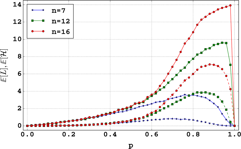
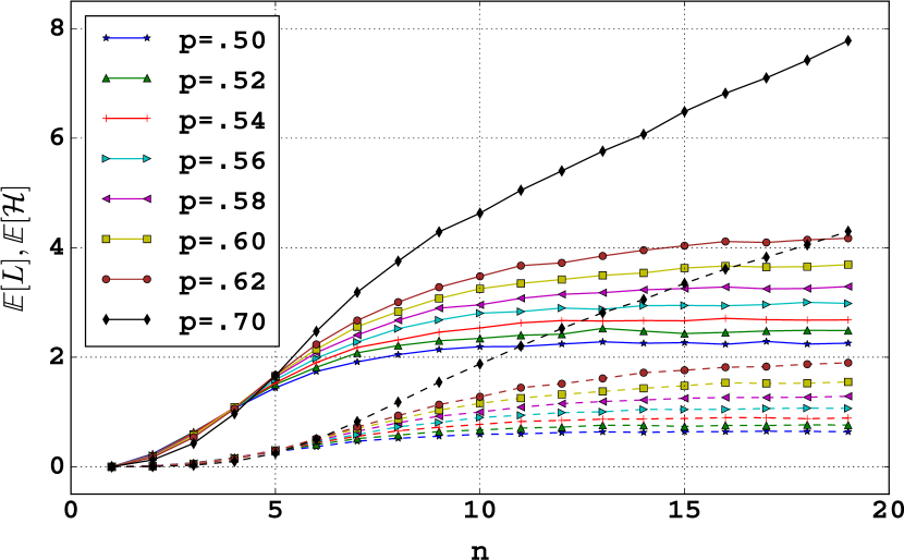
Figure 4: (left) The average codeword length $\mathbb{E}[L]$ depicted by solid lines and average entropy $\mathbb{E}[\mathcal{H}]$ depicted by dash lines versus the percolation density $p$ for three different depths $n=7,12$ and $16$. Note that when $p=1.0$ both quantities drop to zero since there are no leaves present at $p=1.0$. This is expected since there is no information due to randomness at this density. (right) The same quantities versus the maximum depth $n$ for various percolation densities $p$. Again the solid lines represent the average codeword length and the dashed lines represent the average entropy. It is seen that both quantities are bounded as long as $1/2\leq p<1/\sqrt[3]{4}$. For $p=0.7$ observe that they grow exponentially as $n$ grows.

The simulation results are in agreement with the results yielded above. In Fig. 4 on the left pane, the dependence of $\mathbb{E}[L]$ and $\mathbb{E}[\mathcal{H}]$ on the maximum generation (depth) $n$ and the percolation density $p$ are shown. It is observed that the average codeword length and the average entropy versus $p$ monotonically increase until they reach their maximum and then reach the value zero when $p=1.0$. This is due to the fact that when $p=1.0$ there are no leaves that contribute to $L$ and $\mathcal{H}$. Moreover, in the same figure on the right pane, the dependence of $\mathbb{E}[L]$ and $\mathbb{E}[\mathcal{H}]$ on the depth of the simulation is depicted. It is clear that so long $1/2\leq p<\sqrt[3]{1/4}$ both quantities remain finite. To make this stand out, the average codeword length and the entropy at $p=0.7$ are plotted and it is seen that in contrast to the other percolation densities, $\mathbb{E}[L]$ and $\mathbb{E}[\mathcal{H}]$ grow exponentially. In Fig. 5 the average codeword length and the entropy yielded by the simulation results are plotted against their analytical expressions given by Eq. (26) and Eq. (27) respectively. The dashed lines are the analytical expressions describing the asymptotic behaviour of the aforementioned quantities in the limit of $n\rightarrow\infty$. Obviously, there is a gap between the asymptotics yielded by the simulation results due to the fact that while deriving the expressions Eq. (26) and Eq. (27) it was assumed that $\Lambda(\mathcal{C})$ is a constant when $n\rightarrow\infty$ and hence substituted by its means. Yet, for the simulation results, the normalisation factor $\Lambda$ is calculated exactly. Nevertheless, it is still promising to indeed observe the that the average codeword length and the average entropy both remain finite as $n$ increases as long as $1/2\leq p<\sqrt[3]{1/4}$.

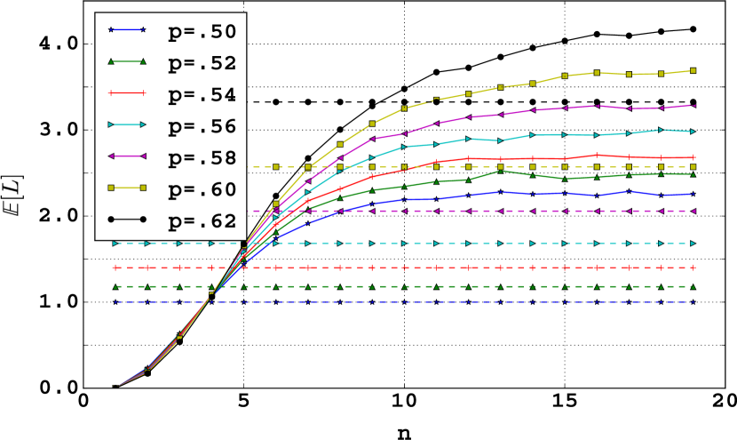
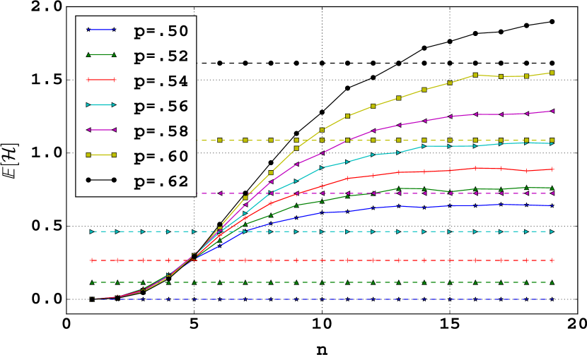
Figure 5: (left) The average codeword length for various percolation densities $p$ versus the depth of the tree $n$. It is seen that $\mathbb{E}[L]$ saturates as long as $1/2\leq p<1/\sqrt[3]{4}$. (right) The same as the left pain but for the average entropy $\mathbb{E}[\mathcal{H}]$ . The solid lines represent the simulation results while the dashed lines are the saturation plateaus predicted by the Eq. (27) and Eq. (26).

4 Conclusion

It is demonstrated here that a given percolation cluster generated via a Bernoulli percolation process on a perfect binary tree can be regarded as an encoding scheme with a set of symbols identified as the leaves of the cluster, along with their associated probabilities satisfying the Bernoulli probability measure. The codewords are simultaneously yielded by traversing the open paths from the root of the tree to their respective leaves. It was proven that with this very configuration, one can still have a set of infinite symbols and keep the amount of the information and the average codeword length finite by choosing the percolation density $p$ appropriately.

One of the aims of this paper was to show that a branching process as simple as Bienaymé-Galton-Watson process could have potential applications in computer science. It may have deep implications in how one algorithmically encodes large data, stores, compresses and also importantly encrypts them. Other non-trivial branching processes may be even found more crucial in shaping our understanding of data integrity and storage or encryption methods that are far challenging to be breached. Also the author wants to note that the Bienaymé-Galton-Watson process has already been used to study some natural processes. For instance in the electron multiplier detector or nuclear chain reactions [21, 22]. Not only limited to these, other processes such as the birth-death process which can be utilised to find the rate at which a new species emerges [23]. It may be that the nature intrinsically encodes the information in such a manner that the entropy remains bounded yet the possible outcomes are infinitely many.

References

- [1] Patrick O’Neil, Edward Cheng, Dieter Gawlick, and Elizabeth O’Neil. The log-structured merge-tree (lsm-tree). Acta Informatica, 33(4):351–385, 1996.
- [2] Pradeep J Shetty, Richard P Spillane, Ravikant R Malpani, Binesh Andrews, Justin Seyster, and Erez Zadok. Building workload-independent storage with vt-trees. In 11th USENIX Conference on File and Storage Technologies (FAST 13), pages 17–30, 2013.
- [3] Ohad Rodeh, Josef Bacik, and Chris Mason. Btrfs: The linux b-tree filesystem. ACM Transactions on Storage (TOS), 9(3):1–32, 2013.
- [4] Goetz Graefe and Harumi Kuno. Modern b-tree techniques. In 2011 IEEE 27th International Conference on Data Engineering, pages 1370–1373. IEEE, 2011.
- [5] David A Huffman. A method for the construction of minimum-redundancy codes. Proceedings of the IRE, 40(9):1098–1101, 1952.
- [6] Henry William Watson and Francis Galton. On the probability of the extinction of families. The Journal of the Anthropological Institute of Great Britain and Ireland, 4:138–144, 1875.
- [7] G. Grimmett. Percolation. Grundlehren der mathematischen Wissenschaften : a series of comprehensive studies in mathematics. Springer Verlag, 1989.
- [8] Wolfgang Bauhofer and Josef Z Kovacs. A review and analysis of electrical percolation in carbon nanotube polymer composites. Composites science and technology, 69(10):1486–1498, 2009.
- [9] Harry Kesten. Percolation theory and first-passage percolation. The Annals of Probability, 15(4):1231–1271, 1987.
- [10] Ahmad Mardoukhi, Yousof Mardoukhi, Mikko Hokka, and Veli-Tapani Kuokkala. Effects of heat shock on the dynamic tensile behavior of granitic rocks. Rock mechanics and rock engineering, 50(5):1171–1182, 2017.
- [11] Dietrich Stauffer. Can percolation theory be applied to the stock market? Annalen der Physik, 7(5-6):529–538, 1998.
- [12] Yao Yu and Jun Wang. Lattice-oriented percolation system applied to volatility behavior of stock market. Journal of Applied Statistics, 39(4):785–797, 2012.
- [13] Thomas Owen Richardson, Kim Christensen, Nigel Rigby Franks, Henrik Jeldtoft Jensen, and Ana Blagovestova Sendova-Franks. Ants in a labyrinth: a statistical mechanics approach to the division of labour. PLoS One, 6(4):e18416, 2011.
- [14] Paulo FF Almeida, Winchil LC Vaz, and TE Thompson. Lateral diffusion and percolation in two-phase, two-component lipid bilayers. topology of the solid-phase domains in-plane and across the lipid bilayer. Biochemistry, 31(31):7198–7210, 1992.
- [15] Kingo Kobayashi, Hiroyoshi Morita, and Mamoru Hoshi. Percolation on a k-ary tree. In General Theory of Information Transfer and Combinatorics, pages 633–638. Springer, 2006.
- [16] Søren Asmussen, Heinrich Hering, et al. Branching processes, volume 3. Springer, 1983.
- [17] Theodore Edward Harris et al. The theory of branching processes, volume 6. Springer Berlin, 1963.
- [18] Michael Drmota. Distribution of the height of leaves of rooted trees. Diskretnaya Matematika, 6(1):67–82, 1994.
- [19] Steven Roman. Introduction to coding and information theory. Springer Science & Business Media, 1996.
- [20] S Cortes Reina, Stephan Foldes, Yousof Mardoukhi, and Navin M Singhi. Note on islands in path-length sequences of binary trees. arXiv preprint arXiv:1409.3855, 2014.
- [21] W Shockley and JR Pierce. A theory of noise for electron multipliers. Proceedings of the Institute of Radio Engineers, 26(3):321–332, 1938.
- [22] D Hawkins and S Ulam. Theory of Multiplicative Process, volume 287. Atomic Energy Commission, 1946.
- [23] George Udny Yule. Ii.—a mathematical theory of evolution, based on the conclusions of dr. jc willis, fr s. Philosophical transactions of the Royal Society of London. Series B, containing papers of a biological character, 213(402-410):21–87, 1925.