Stability and convergence of Strang splitting. Part II: Tensorial Allen-Cahn equations

Abstract.

We consider the second-order in time Strang-splitting approximation for tensorial (e.g. vector-valued and matrix-valued) Allen-Cahn equations. Both the linear propagator and the nonlinear propagator are computed explicitly. For the vector-valued case, we prove the maximum principle and unconditional energy dissipation for a judiciously modified energy functional. The modified energy functional is close to the classical energy up to $\mathcal{O}(\tau)$ where $\tau$ is the splitting step. For the matrix-valued case, we prove a sharp maximum principle in the matrix Frobenius norm. We show modified energy dissipation under very mild splitting step constraints. We exhibit several numerical examples to show the efficiency of the method as well as the sharpness of the results.

1. Introduction

In this work we investigate the stability of second-order in time Strang-splitting methods applied to two models: One is the vector-valued Allen-Cahn (AC) equation, and the other is the matrix-valued Allen-Cahn system. The operator splitting methods have been extensively used in the numerical simulation of many physical problems, including phase-field equations [2, 3, 13, 14, 15, 17, 16, 12], Schrödinger equations [4, 5, 20], and the reaction-diffusion systems [6, 9]. A prototypical second order in time method is the Strang splitting approximation [10, 11]. In a slightly more general set up, we consider the following abstract parabolic problem:

$$\begin{cases}\partial_{t}u=\mathcal{L}u-f(u),\quad t>0;\\ u\Bigr{|}_{t=0}=u_{0}.\end{cases}$$ (1.1)

where $u:[0,\infty)\to\mathbb{B}$ and $\mathbb{B}$ is a real Banach space. The operator $\mathcal{L}:\;\mathcal{D}(\mathcal{L})\subset\mathbb{B}\to\mathbb{B}$ is a dissipative closed operator which typically is the infinitesimal generator of a strongly-continuous dissipative semigroup. The domain $\mathcal{D}(\mathcal{L})$ is typically a dense subset of $\mathbb{B}$. On the other hand $f:\,\mathbb{B}\to\mathbb{B}$ is a nonlinear operator. Take $\tau>0$ as the splitting time step. Define for $t>0$,

$$\mathcal{S}_{\mathcal{L}}^{(\mathbb{B})}(t)=e^{t\mathcal{L}},$$ (1.2)

which is the solution operator to the linear equation $\partial_{t}u=\mathcal{L}u$. Define $\mathcal{S}_{\mathcal{N}}^{(\mathbb{B})}(\tau)$ as the nonlinear solution operator to the system

$$\begin{cases}\partial_{t}u=-f(u),\;0<t\leq\tau;\\ u\Bigr{|}_{t=0}=b\in\mathbb{B}.\end{cases}$$ (1.3)

In yet other words, $\mathcal{S}_{\mathcal{N}}^{(\mathbb{B})}(\tau)$ is the map $b\to u(\tau)$. The Strang-splitting approximation for (1.1) takes the form

$$u^{n+1}=\mathcal{S}^{(\mathbb{B})}_{\mathcal{L}}(\tau/2)\mathcal{S}^{(\mathbb{B})}_{\mathcal{N}}(\tau)\mathcal{S}_{\mathcal{L}}^{(\mathbb{B})}(\tau/2)u^{n},\quad n\geq 0.$$ (1.4)

Let $u^{\mathrm{ex}}$ be the exact solution to (1.1). In general it is expected that on a finite time interval $[0,T]$

$$\sup_{n\tau\leq T}\|u^{\mathrm{ex}}(n\tau)-u^{n}\|=\mathcal{O}(\tau^{2}),$$ (1.5)

where $\|\cdot\|$ denotes a working norm which is allowed to be weaker than the norm endowed with the Banach space $\mathbb{B}$. On the other hand, the local truncation error is typically $\mathcal{O}(\tau^{3})$, i.e.

$$\|\mathcal{S}^{\mathrm{ex}}(\tau)a-\mathcal{S}^{(\mathbb{B})}_{\mathcal{L}}(\tau/2)\mathcal{S}^{(\mathbb{B})}_{\mathcal{N}}(\tau)\mathcal{S}_{\mathcal{L}}^{(\mathbb{B})}(\tau/2)a\|=\mathcal{O}(\tau^{3}),$$ (1.6)

where $a\in\mathbb{B}$, and $\mathcal{S}^{\mathrm{ex}}(\tau)$ is the exact solution operator to (1.1).

Despite the remarkable effectiveness of the scheme (1.4) (cf. [3] for the case of Allen-Cahn equations), there have been few rigorous works addressing the stability and regularity of the Strang splitting solutions. The general assertions (1.5)–(1.6) are hinged on nontrivial a priori estimates of the numerical iterates in various Banach spaces. In a recent series of works [13, 14, 15, 16, 17], we developed a new theoretical framework to establish convergence, stability and regularity of general operator splitting methods for a myriad of phase field models including the Cahn-Hilliard equations, Allen-Cahn equations and the like. More pertinent to the discussion here is the recent work [16] which settled the stability for a class of scalar-valued Allen-Cahn equations with polynomial or logarithmic potential nonlinearities.

In this work we develop further the program initiated in [16] and analyze the Strang-splitting for two types of tensorial Allen-Cahn equations. The first model is the vector-valued Allen-Cahn equation

$$\partial_{t}{\mathbf{u}}=\Delta\mathbf{u}+(1-|\mathbf{u}|^{2})\mathbf{u},\quad\mathbf{u}\in\mathbb{R}^{m},$$ (1.7)

where $|\mathbf{u}|^{2}=\sum_{i=1}^{m}u_{i}^{2}$ for $\mathbf{u}=(u_{1},\cdots,u_{m})^{\mathrm{T}}$ ($m\geq 1$ is an integer), and the Laplacian operator is applied to $\mathbf{u}$ component-wise. In particular, when $m=2$, the vector-valued Allen-Cahn equation is equivalent to the complex-valued Ginzburg–Landau model for superconductivity (cf. [7, 8] using a standard transformation $\psi(x)=e^{iA\cdot x}u(x)$ and identifying $u=u_{1}+iu_{2}$). The second model is the matrix-valued Allen-Cahn equation:

$$\partial_{t}U=\Delta U+U-UU^{\mathrm{T}}U,\quad U\in\mathbb{R}^{m\times m},$$ (1.8)

where the Laplacian operator is applied to the matrix $U$ entry-wise. The matrix-valued Allen-Cahn is introduced in [18] to find stationary points of the Dirichlet energy for orthogonal matrix-valued fields, that can be used in inverse problems in image analysis and directional field synthesis problems etc. For both models we shall develop the corresponding stability theory for the Strang-splitting approximation in the style of (1.4). Roughly speaking, our results can be summarized in the following table where $\tau$ is the splitting time step.

	$L^{\infty}$-stability	Modified energy dissipation
Vector-valued AC	$0<\tau<\infty$	$0<\tau<\infty$
Matrix-valued AC	$0<\tau<\infty$	$me^{\tau}(e^{2\tau}-1)\leq 0.43$

We turn now to more precise formulation of the results. Our first result is on the vector-valued Allen-Cahn equation. An interesting feature is that the nonlinear propagator still enjoys a relatively simple explicit expression.

Theorem 1.1 (Unconditional stability of Strang-splitting for the vector-valued AC).

Suppose $\Omega=[-\pi,\pi]^{d}$ is the $2\pi$-periodic $d$-dimensional torus in physical dimensions $d\leq 3$. Consider the vector-valued AC for $\mathbf{u}:\,[0,\infty)\times\Omega\to\mathbb{R}^{m}$, $m\geq 1$:

$$\begin{cases}\partial_{t}\mathbf{u}=\Delta\mathbf{u}+(1-|\mathbf{u}|^{2})\mathbf{u},\quad(t,x)\in(0,\infty)\times\Omega;\\ \mathbf{u}\Bigr{|}_{t=0}=\mathbf{u}^{0},\end{cases}$$ (1.9)

where $\mathbf{u}^{0}:\,\Omega\to\mathbb{R}^{m}$ is the initial data. Define $\mathcal{S}_{\mathcal{L}}(t)=e^{t\Delta}$ and for $\mathbf{w}\in\mathbb{R}^{m}$,

$$\mathcal{S}_{\mathcal{N}}(t)\mathbf{w}\coloneqq\left((e^{2t}-1)|\mathbf{w}|^{2}+1\right)^{-\frac{1}{2}}e^{t}\mathbf{w}.$$ (1.10)

Define for $n\geq 0$ the Strang-splitting iterates

$$\mathbf{u}^{n+1}=\mathcal{S}_{\mathcal{L}}\left(\tau/2\right)\mathcal{S}_{\mathcal{N}}\left(\tau\right)\mathcal{S}_{\mathcal{L}}\left(\tau/2\right)\mathbf{u}^{n}.$$ (1.11)

The following hold.

1. The maximum principle. For any $\tau>0$ and any $n\geq 0$, it holds that

   $$\||\mathbf{u}^{n+1}|\|_{L_{x}^{\infty}}\leq\max\{1,\;\||\mathbf{u}^{n}|\|_{L_{x}^{\infty}}\}.$$ (1.12)

   It follows that

   $$\sup_{n\geq 1}\||\mathbf{u}^{n}|\|_{L_{x}^{\infty}}\leq\max\{1,\;\||\mathbf{u}^{0}|\|_{L_{x}^{\infty}}\}.$$ (1.13)

   In particular if $\||\mathbf{u}^{0}|\|_{L_{x}^{\infty}}\leq 1$, then

   $$\sup_{n\geq 1}\||\mathbf{u}^{n}|\|_{L_{x}^{\infty}}\leq 1.$$ (1.14)

2. Modified energy dissipation. For any $\tau>0$, we have

   $$\widetilde{E}(\tilde{\mathbf{u}}^{n+1})\leq\widetilde{E}(\tilde{\mathbf{u}}^{n}),\quad\forall\,n\geq 0.$$ (1.15)

   Here

   $$\tilde{\mathbf{u}}^{n}=\mathcal{S}_{\mathcal{L}}\left(\tau/2\right)\mathbf{u}^{n};$$ (1.16)

   $$\widetilde{E}({\mathbf{u}})=\int_{\Omega}\left(\frac{1}{2\tau}\left\langle(e^{-\tau\Delta}-1){\mathbf{u}},{\mathbf{u}}\right\rangle+G({\mathbf{u}})\right)\,dx;$$ (1.17)

   $$G(\mathbf{u})=\frac{1}{2\tau}|\mathbf{u}|^{2}-\frac{e^{\tau}}{\tau(e^{2\tau}-1)}\left(\left(1+(e^{2\tau}-1)|\mathbf{u}|^{2}\right)^{\frac{1}{2}}-1\right).$$ (1.18)

   In the above $\langle\mathbf{a},\,\mathbf{b}\rangle=\sum_{i=1}^{m}a_{i}b_{i}$ for $\mathbf{a}=(a_{1},\cdots,a_{m})^{\mathrm{T}}$, $\mathbf{b}=(b_{1},\cdots,b_{m})^{\mathrm{T}}\in\mathbb{R}^{m}$.

Remark 1.1.

The significance of the uniform stability result obtained in Theorem 1.1 is that it leads to all higher Sobolev estimates as well as convergence. For example, by using the techniques developed in [16], we can show uniform Sobolev bounds. Namely if $\mathbf{u}^{0}\in H^{k_{0}}(\Omega,\,\mathbb{R}^{m})$ for some $k_{0}\geq 1$, then

$$\sup_{n\geq 1}\|\mathbf{u}^{n}\|_{H^{k_{0}}}\leq C_{1},$$ (1.19)

where $C_{1}>0$ depends only on ($k_{0}$, $d$, $\|u^{0}\|_{H^{k_{0}}}$, $m$). Moreover for any $k\geq k_{0}$, we have

$$\sup_{n\geq\frac{1}{\tau}}\|\mathbf{u}^{n}\|_{H^{k}}\leq C_{2},$$ (1.20)

where $C_{2}>0$ depends only on ($m$, $k$, $k_{0}$, $d$, $\|u^{0}\|_{H^{k_{0}}}$). Let $\mathbf{u}^{\mathrm{ex}}$ be the exact solution to the vector-valued Allen-Cahn equation corresponding to initial data $\mathbf{u}^{0}$. If we assume $\mathbf{u}^{0}$ has high regularity (e.g. $\mathbf{u}^{0}\in H^{k_{0}}$ for some sufficiently large $k_{0}$), then for any $T>0$, it holds that

$$\sup_{n\geq 1,n\tau\leq T}\|\mathbf{u}^{n}-\mathbf{u}^{\mathrm{ex}}(n\tau,\cdot)\|_{L^{2}(\Omega)}\leq C\cdot\tau^{2},$$ (1.21)

where $C>0$ depends on ($\mathbf{u}^{0}$, $T$, $d$, $m$).

Remark 1.2.

The modified energy for $\mathbf{u}^{n}$ has a close connection with the standard energy $E^{\mathrm{st}}(\mathbf{u}^{n})$ defined by

$$E^{\mathrm{st}}(\mathbf{u}^{n})=\int_{\Omega}\left(\frac{1}{2}|\nabla\mathbf{u}^{n}|^{2}+\frac{1}{4}(|\mathbf{u}^{n}|^{2}-1)^{2}-\frac{1}{4}\right)\,dx.$$ (1.22)

Note that here the integrand of $E^{\mathrm{st}}(\cdot)$ includes a harmless constant $-\frac{1}{4}$. If $\mathbf{u}^{0}\in H^{k_{0}}(\Omega,\mathbb{R}^{m})$ for sufficiently large $k_{0}$, then for $0<\tau\leq 1$, we have

$$\sup_{n\geq 0}|\widetilde{E}^{n}-E^{\mathrm{st}}(\mathbf{u}^{n})|\leq C_{3}\tau,$$ (1.23)

where $C_{3}>0$ depends only on ($d$, $m$, $\mathbf{u}^{0}$). This result can be proved by using the uniform Sobolev estimates established in the preceding remark. We omit the elementary argument here for simplicity.

In recent work [18], Osting and Wang considered the minimization problem

$$\min_{A\in H^{1}(\Omega,O_{m})}\frac{1}{2}\int_{\Omega}\|\nabla A\|_{F}^{2}\,dx,$$ (1.24)

where $O_{m}\subset\mathbb{R}^{m\times m}$ is the group of orthogonal matrices, and the gradient is taken as the usual sense when $A$ is regarded as a matrix-valued function in $\mathbb{R}^{m\times m}$, i.e. not the covariant derivative sense in e.g. [1]. For a matrix $A,B\in\mathbb{R}^{m\times m}$, we use the usual Frobenius norm and Frobenius inner product:

$$\|A\|_{F}^{2}=\sum_{i,j=1}^{m}A_{ij}^{2},\quad\langle A,B\rangle_{F}=\sum_{i,j=1}^{m}A_{ij}B_{ij}.$$ (1.25)

To enforce the hard constraint $A\in H^{1}(\Omega,O_{m})$, one can employ two relaxed functionals parametrized by $0<\epsilon\ll 1$:

$$\text{Model 1}:\quad\min_{A\in H^{1}(\Omega,\mathbb{R}^{m\times m})}\int_{\Omega}\left(\frac{1}{2}\|\nabla A\|_{F}^{2}+\frac{1}{2\epsilon^{2}}\mathrm{dist}^{2}(O_{n},A)\right)\,dx;$$ (1.26)

$$\text{Model 2}:\quad\min_{A\in H^{1}(\Omega,\mathbb{R}^{m\times m})}\int_{\Omega}\left(\frac{1}{2}\|\nabla A\|_{F}^{2}+\frac{1}{4\epsilon^{2}}\|A^{\mathrm{T}}A-\mathrm{I}_{m}\|_{F}^{2}\right)\,dx.$$ (1.27)

As shown in [18], these in turn lead to the following gradient flows

$$\text{Model 1}:\quad\partial_{t}A=\Delta A-\epsilon^{-2}U(\Sigma-\mathrm{I}_{m})V^{\mathrm{T}};$$ (1.28)

$$\text{Model 2}:\quad\partial_{t}A=\Delta A-\epsilon^{-2}U(\Sigma^{2}-\mathrm{I}_{m})\Sigma V^{\mathrm{T}},$$ (1.29)

where $A=U\Sigma V^{\mathrm{T}}$ is the singular value decomposition of the nonsingular matrix $A$. The gradient flow in Model 2 can be further simplified as

$$\partial_{t}A=\Delta A-\epsilon^{-2}A(A^{\mathrm{T}}A-\mathrm{I}_{m}).$$ (1.30)

In [18], the authors introduced an energy-splitting method to find local minima of (1.26) and (1.27). These are nontrivial stationary solutions other than the trivial constant orthogonal matrix-valued function) of (1.28) and (1.30). The method can be rephrased as the following operator-splitting:

$$U^{n+1}=\mathcal{S}_{\mathcal{N}}^{\mathrm{Proj}}\mathcal{S}_{\mathcal{L}}(\tau)U^{n},$$ (1.31)

where $S_{\mathcal{L}}(\tau)=e^{\tau\Delta}$ is applied to the matrix entry-wise, and

$$\Bigl{(}\mathcal{S}_{\mathcal{N}}^{\mathrm{Proj}}A\Bigr{)}(x)=U(x)V^{\mathrm{T}}(x),\qquad\text{if $A(x)=U(x)\Sigma(x)V^{\mathrm{T}}(x)$}.$$ (1.32)

In this work, we take a direct approach to (1.30) and employ a Strang-splitting method to solve (1.30) efficiently and accurately. For simplicity of presentation we shall take $\epsilon=1$ in (1.30). We have the following theorem.

Theorem 1.2 (Stability for matrix-valued AC).

Suppose $\Omega=[-\pi,\pi]^{d}$ is the $2\pi$-periodic $d$-dimensional torus in physical dimensions $d\leq 3$. Consider the matrix-valued AC for $U:\,[0,\infty)\times\Omega\to\mathbb{R}^{m\times m}$, $m\geq 1$:

$$\begin{cases}\partial_{t}U=\Delta U+U-UU^{\mathrm{T}}U,\quad(t,x)\in(0,\infty)\times\Omega;\\ U\Bigr{|}_{t=0}=U^{0},\end{cases}$$ (1.33)

where $U^{0}:\,\Omega\to\mathbb{R}^{m\times m}$ is the initial data. Define $\mathcal{S}_{\mathcal{L}}(t)=e^{t\Delta}$ and for $A\in\mathbb{R}^{m\times m}$,

$$\mathcal{S}_{\mathcal{N}}(t)A\coloneqq\left((e^{2t}-1)AA^{\mathrm{T}}+I\right)^{-\frac{1}{2}}e^{t}A.$$ (1.34)

Define for $n\geq 0$ the Strang-splitting iterates

$$U^{n+1}=\mathcal{S}_{\mathcal{L}}\left(\tau/2\right)\mathcal{S}_{\mathcal{N}}\left(\tau\right)\mathcal{S}_{\mathcal{L}}\left(\tau/2\right)U^{n}.$$ (1.35)

The following hold.

1. The maximum principle. For any $\tau>0$ and any $n\geq 0$, it holds that

   $$\|\|U^{n+1}\|_{F}\|_{L_{x}^{\infty}}\leq\max\{\sqrt{m},\;\|\|U^{n}\|_{F}\|_{L_{x}^{\infty}}\}.$$ (1.36)

   It follows that

   $$\sup_{n\geq 1}\|\|U^{n}\|_{F}\|_{L_{x}^{\infty}}\leq\max\{\sqrt{m},\;\|\|U^{0}\|_{F}\|_{L_{x}^{\infty}}\}.$$ (1.37)

   In particular if $\|\|U^{0}\|_{F}\|_{L_{x}^{\infty}}\leq\sqrt{m}$, then

   $$\sup_{n\geq 1}\|\|U^{n}\|_{F}\|_{L_{x}^{\infty}}\leq\sqrt{m}.$$ (1.38)

2. Modified energy dissipation for small time. Assume $\|\|U^{0}\|_{F}\|_{L_{x}^{\infty}}\leq\sqrt{m}$. If $\tau>0$ satisfies

   $$me^{\tau}(e^{2\tau}-1)\leq 0.43,$$ (1.39)

   then

   $$\widetilde{E}(\tilde{U}^{n+1})\leq\widetilde{E}(\tilde{U}^{n}),\quad\forall\,n\geq 0.$$ (1.40)

   Here

   $$\tilde{U}^{n}=\mathcal{S}_{\mathcal{L}}\left(\tau/2\right)U^{n};$$ (1.41)

   $$\widetilde{E}({U})=\int_{\Omega}\frac{1}{2\tau}\left\langle(e^{-\tau\Delta}-1){U},{U}\right\rangle_{F}+\left\langle G({U}),I\right\rangle_{F}\,dx;$$ (1.42)

   $$G(U)=\frac{1}{2\tau}UU^{\mathrm{T}}-\frac{e^{\tau}}{\tau(e^{2\tau}-1)}\left(\left(\mathrm{I}+(e^{2\tau}-1)UU^{\mathrm{T}}\right)^{\frac{1}{2}}-\mathrm{I}\right).$$ (1.43)

   In the above $\langle A,B\rangle_{F}=\mathrm{Tr}(A^{\mathrm{T}}B)=\sum_{i,j}A_{ij}B_{ij}$ denotes the usual Frobenius inner product.

Remark 1.3.

We should point it out that the dynamics of the matrix-valued Allen-Cahn case are in general qualitatively different from the vector-valued Allen-Cahn case. In particular there does not appear to exist a simple procedure such that the vector-valued AC model can be embedded into the matrix-valued AC model. A very tempting idea is to consider the following system

$$\begin{cases}\partial_{t}U=\Delta U+U-UU^{\mathrm{T}}U,\\ U\Bigr{|}_{t=0}=U^{0}=\mathbf{a}{\mathbf{a}}^{\mathrm{T}},\end{cases}$$ (1.44)

where $\mathbf{a}:\,\Omega\to\mathbb{R}^{m}$. In yet other words, we consider the matrix-valued AC model with rank one initial data. It is natural to speculate that $U$ is connected with the solution to

$$\begin{cases}\partial_{t}\mathbf{u}=\Delta\mathbf{u}+\mathbf{u}-|\mathbf{u}|^{2}\mathbf{u},\\ \mathbf{u}\Bigr{|}_{t=0}=\mathbf{a}.\end{cases}$$ (1.45)

However one can check that $U\neq\mathbf{u}{\mathbf{u}}^{\mathrm{T}}$ for $t>0$. The main reason is that

$$e^{t\Delta}\Bigl{(}\mathbf{a}{\mathbf{a}}^{\mathrm{T}}\Bigr{)}\neq{e^{t\Delta}\mathbf{a}}({e^{t\Delta}\mathbf{a}})^{\mathrm{T}}.$$ (1.46)

If one drops the Laplacian and adopt only the nonlinear evolution, then one can show that $U={\mathbf{u}}{\mathbf{u}}^{\mathrm{T}}$.

The rest of this article is organized as follows. In Section 2 we carry out the proof of Theorem 1.1. In Section 3 we analyze the Strang-splitting for the matrix-valued Allen-Cahn equation. In Section 4 we showcase a few numerical simulations for the vector-valued Allen-Cahn and the matrix-valued Allen-Cahn equations.

2. Vector-valued Allen-Cahn

In this section we give the proof of Theorem 1.1. We consider the vector-valued Allen-Cahn equation for $\mathbf{u}=\mathbf{u}(t,x):\,[0,\infty)\times\Omega\to\mathbb{R}^{m}$, $m\geq 1$:

$$\begin{cases}\partial_{t}\mathbf{u}=\Delta\mathbf{u}+\mathbf{u}-|\mathbf{u}|^{2}\mathbf{u},\qquad(t,x)\in(0,\infty)\times\Omega;\\ \mathbf{u}\Bigr{|}_{t=0}=\mathbf{u}^{0},\quad x\in\Omega.\end{cases}$$ (2.1)

Here $|\mathbf{u}|^{2}$ is the usual $l^{2}$ norm, i.e. $|\mathbf{u}|^{2}=\sum_{i=1}^{m}u_{i}^{2}$ for $\mathbf{u}=(u_{1},\cdots,u_{m})^{\mathrm{T}}$. The spatial domain $\Omega=[-\pi,\,\pi]^{d}$ is the $2\pi$-periodic torus in physical dimensions $d\leq 3$.

We proceed in several steps.

2.1. Properties of $\mathcal{S}_{\mathcal{L}}$ and $\mathcal{S}_{\mathcal{N}}$

We first consider the pure nonlinear evolution. This is driven by the following ODE system written for $\mathbf{u}=\mathbf{u}(t):\,[0,\infty)\to\mathbb{R}^{m}$.

$$\begin{cases}\frac{d}{dt}{\mathbf{u}}=(1-|\mathbf{u}|^{2})\mathbf{u},\\ \mathbf{u}\Bigr{|}_{t=0}=\mathbf{a}\in\mathbb{R}^{m}.\end{cases}$$ (2.2)

Proposition 2.1 (The explicit nonlinear propagator $\mathcal{S}_{\mathcal{N}}(t)$).

Given $\mathbf{a}\in\mathbb{R}^{m}$, the unique smooth solution $U(t)$ to (2.2) is given by

$$\mathcal{S}_{\mathcal{N}}(t)\mathbf{a}:=U(t)=\left((e^{2t}-1)|\mathbf{a}|^{2}+1\right)^{-\frac{1}{2}}e^{t}\mathbf{a},\qquad t>0.$$ (2.3)

Remark 2.1.

If $\mathbf{a}$ is a vector-valued function, i.e. $\mathbf{a}:\,\Omega\to\mathbb{R}^{m}$, then we naturally extend the definition of $\mathcal{S}_{\mathcal{N}}(t)\mathbf{a}$ as

$$\Bigl{(}\mathcal{S}_{\mathcal{N}}(t)\mathbf{a}\Bigr{)}(x)=\mathcal{S}_{\mathcal{N}}(t)(\mathbf{a}(x)),\quad x\in\Omega.$$ (2.4)

This convention will be used without explicit mentioning.

Proof.

Taking the $l^{2}$-inner product on both sides of (2.2) gives us

$$\frac{1}{2}\frac{d}{dt}|{\mathbf{u}}|^{2}=(1-|\mathbf{u}|^{2})|{\mathbf{u}}|^{2}.$$ (2.5)

This is an ODE for $|\mathbf{u}|^{2}$ which has an explicit solution:

$$|\mathbf{u}(t)|^{2}=\frac{e^{2t}|\mathbf{a}|^{2}}{(e^{2t}-1)|\mathbf{a}|^{2}+1}.$$ (2.6)

Plugging the above into (2.2), we obtain

$$\frac{d}{dt}{\mathbf{u}}=\frac{1-|\mathbf{a}|^{2}}{(e^{2t}-1)|\mathbf{a}|^{2}+1}\mathbf{u}.$$ (2.7)

It is not difficult to work out the explicit solution as

$$\mathbf{u}(t)=\frac{e^{t}\mathbf{a}}{\left((e^{2t}-1)|\mathbf{a}|^{2}+1\right)^{\frac{1}{2}}}.$$ (2.8)

∎

Given $\mathbf{u}=(u_{1},\cdots,u_{m})^{\mathrm{T}}:\,\Omega\to\mathbb{R}^{m}$ and $t>0$, we define the linear propagator

$$\Bigl{(}\mathcal{S}_{\mathcal{L}}(t)\mathbf{u}\Bigr{)}_{i}(x)=(e^{t\Delta}u_{i})(x),\qquad i=1,\cdots,m.$$ (2.9)

In yet other words, the operator $\mathcal{S}_{\mathcal{L}}(t)=e^{t\Delta}$ is applied to the vector $\mathbf{u}$ entry-wise.

Theorem 2.1 (Maximum principle for $\mathcal{S}_{\mathcal{L}}$ and $\mathcal{S}_{\mathcal{N}}$).

Let $\Omega=[-\pi,\pi]^{d}$ be the $2\pi$-periodic $d$-dimensional torus. For any $\tau>0$, the following hold.

1. For any measurable vector-valued $\mathbf{a}:\,\Omega\to\mathbb{R}^{m}$, we have

   $$\||\mathcal{S}_{\mathcal{L}}(\tau)\mathbf{a}|\|_{L_{x}^{\infty}}\leq\||\mathbf{a}(x)|\|_{L_{x}^{\infty}}.$$ (2.10)

2. For any $\mathbf{w}\in\mathbb{R}^{m}$, we have

   $$|\mathcal{S}_{\mathcal{N}}(\tau)\mathbf{w}|\leq\max\{1,\,|\mathbf{w}|\}.$$ (2.11)

Proof.

We first show (2.10). Clearly for any vector $\mathbf{v}\in\mathbb{R}^{m}$, we have

$$|\mathbf{v}|=\sup_{\tilde{\mathbf{v}}\in\mathbb{R}^{m}:\;|\tilde{\mathbf{v}}|\leq 1}\langle\mathbf{v},\,\mathbf{\tilde{v}}\rangle,$$ (2.12)

where $\langle,\rangle$ denotes the usual $l^{2}$-inner product. With no loss we may assume $\||\mathbf{a}(x)|\|_{L_{x}^{\infty}}\leq 1$. Fix $x_{0}\in\Omega$. It suffices for us to show

$$\left|\int_{\Omega}k(x_{0}-y)\mathbf{a}(y)dy\right|\leq 1,$$ (2.13)

where $k(\cdot)$ is the scalar-valued kernel corresponding to $\mathcal{S}_{\mathcal{L}}(\tau)$. By (2.12), we only need to check for any $\tilde{\mathbf{v}}$ with $|\tilde{\mathbf{v}}|\leq 1$,

$$\int_{\Omega}k(x_{0}-y)\langle\mathbf{a}(y),\,\tilde{\mathbf{v}}\rangle dy\leq 1.$$ (2.14)

But this is obvious since $\int_{\Omega}k(x_{0}-y)dy=1$ and $\langle\mathbf{a}(y),\tilde{\mathbf{v}}\rangle\leq\||\mathbf{a}(x)|\|\|_{L_{x}^{\infty}}|\tilde{\mathbf{v}}|\leq 1$.

We turn now to (2.11). By (2.6), we have

$$|\mathcal{S}_{\mathcal{N}}(t)\mathbf{w}|^{2}=\frac{e^{2t}|\mathbf{w}|^{2}}{(e^{2t}-1)|\mathbf{w}|^{2}+1}.$$ (2.15)

Consider the scalar function

$$\varphi(\lambda)=\frac{e^{2t}\lambda}{(e^{2t}-1)\lambda+1}.$$ (2.16)

It is not difficult to check that $\varphi$ is monotonically increasing on $[0,\infty)$. Furthermore if $\lambda\geq 1$, then

$$\varphi(\lambda)\leq\frac{e^{2t}\lambda}{(e^{2t}-1)+1}=\lambda.$$ (2.17)

The desired result clearly follows. ∎

Lemma 2.1.

Let $\tau>0$ and consider $G:\,\mathbb{R}^{m}\to\mathbb{R}$ defined as

$$G(\mathbf{u})=\frac{1}{2\tau}|\mathbf{u}|^{2}-\frac{e^{\tau}}{\tau(e^{2\tau}-1)}\left(\left(1+(e^{2\tau}-1)|\mathbf{u}|^{2}\right)^{\frac{1}{2}}-1\right).$$ (2.18)

For any $\mathbf{u},\mathbf{v}\in\mathbb{R}^{m}$, it holds that

$$-\langle(\nabla G)(\mathbf{u}),\,\mathbf{v}-\mathbf{u}\rangle\leq G(\mathbf{u})-G(\mathbf{v})+\frac{1}{2\tau}|\mathbf{v}-\mathbf{u}|^{2}.$$ (2.19)

Here $\langle\mathbf{a},\,\mathbf{b}\rangle=\sum_{i=1}^{m}a_{i}b_{i}$ for $\mathbf{a}=(a_{1},\cdots,a_{m})^{\mathrm{T}}$, $\mathbf{b}=(b_{1},\cdots,b_{m})^{\mathrm{T}}\in\mathbb{R}^{m}$.

Proof.

We first examine the auxiliary function

$$h(\mathbf{u})=-(1+|\mathbf{u}|^{2})^{\frac{1}{2}}.$$ (2.20)

Clearly

$$\partial_{i}h =-(1+|\mathbf{u}|^{2})^{-\frac{1}{2}}u_{i};$$ (2.21)

$$\partial_{ij}h =(1+|\mathbf{u}|^{2})^{-\frac{3}{2}}u_{i}u_{j}-(1+|\mathbf{u}|^{2})^{-\frac{1}{2}}\delta_{ij}$$ (2.22)

$$=(1+|\mathbf{u}|^{2})^{-\frac{1}{2}}\Bigl{(}\frac{u_{i}}{\sqrt{1+|\mathbf{u}|^{2}}}\frac{u_{j}}{\sqrt{1+|\mathbf{u}|^{2}}}-\delta_{ij}\Bigr{)}.$$ (2.23)

Thus

$$\sum_{i,j=1}^{m}\xi_{i}\xi_{j}\partial_{ij}h\leq 0,\qquad\forall\,\mathbf{\xi}=(\xi_{1},\cdots,\xi_{m})^{\mathrm{T}}\in\mathbb{R}^{m},\;\forall\,\mathbf{u}\in\mathbb{R}^{m}.$$ (2.24)

In yet other words, the function $h$ is concave. Our desired result then easily follows from Taylor expanding $G(\mathbf{u}+\theta(\mathbf{v}-\mathbf{u}))$ for $\theta\in[0,1]$. ∎

Theorem 2.2 (Unconditional modified energy dissipation for vector-valued Allen-Cahn).

Suppose $\Omega=[-\pi,\pi]^{d}$ is the $2\pi$-periodic $d$-dimensional torus in physical dimensions $d\leq 3$. Let $\mathbf{u}^{0}:\;\Omega\to\mathbb{R}^{m}$ satisfy $\||\mathbf{u}^{0}(x)|\|\|_{L^{\infty}_{x}}\leq 1$. Recall $\mathcal{S}_{\mathcal{L}}(t)=e^{t\Delta}$ and for $\mathbf{w}\in\mathbb{R}^{m}$,

$$\mathcal{S}_{\mathcal{N}}(t)\mathbf{w}\coloneqq\left((e^{2t}-1)|\mathbf{w}|^{2}+1\right)^{-\frac{1}{2}}e^{t}\mathbf{w}.$$ (2.25)

Define for $n\geq 0$ the Strang-splitting iterates

$$\mathbf{u}^{n+1}=\mathcal{S}_{\mathcal{L}}\left(\tau/2\right)\mathcal{S}_{\mathcal{N}}\left(\tau\right)\mathcal{S}_{\mathcal{L}}\left(\tau/2\right)\mathbf{u}^{n}.$$ (2.26)

For any $\tau>0$, we have

$$\widetilde{E}(\tilde{\mathbf{u}}^{n+1})\leq\widetilde{E}(\tilde{\mathbf{u}}^{n}),\quad\forall\,n\geq 0,$$ (2.27)

where

$$\tilde{\mathbf{u}}^{n}=\mathcal{S}_{\mathcal{L}}\left(\tau/2\right)\mathbf{u}^{n};$$ (2.28)

$$\widetilde{E}({\mathbf{u}})=\int_{\Omega}\left(\frac{1}{2\tau}\left\langle(e^{-\tau\Delta}-1){\mathbf{u}},{\mathbf{u}}\right\rangle+G({\mathbf{u}})\right)\,dx;$$ (2.29)

$$G(\mathbf{u})=\frac{1}{2\tau}|\mathbf{u}|^{2}-\frac{e^{\tau}}{\tau(e^{2\tau}-1)}\left(\left(1+(e^{2\tau}-1)|\mathbf{u}|^{2}\right)^{\frac{1}{2}}-1\right).$$ (2.30)

In the above $\langle\mathbf{a},\,\mathbf{b}\rangle=\sum_{i=1}^{m}a_{i}b_{i}$ for $\mathbf{a}=(a_{1},\cdots,a_{m})^{\mathrm{T}}$, $\mathbf{b}=(b_{1},\cdots,b_{m})^{\mathrm{T}}\in\mathbb{R}^{m}$.

Proof.

By definition we have

$$e^{-\tau\Delta}\tilde{\mathbf{u}}^{n+1}=\frac{e^{\tau}\tilde{\mathbf{u}}^{n}}{\left((e^{2\tau}-1)|\tilde{\mathbf{u}}^{n}|^{2}+1\right)^{\frac{1}{2}}}.$$ (2.31)

We rewrite it as

$$\frac{1}{\tau}(e^{-\tau\Delta}-1)\tilde{\mathbf{u}}^{n+1}+\frac{1}{\tau}(\tilde{\mathbf{u}}^{n+1}-\tilde{\mathbf{u}}^{n})=\frac{1}{\tau}\left(\frac{e^{\tau}\tilde{\mathbf{u}}^{n}}{\left((e^{2\tau}-1)|\tilde{\mathbf{u}}^{n}|^{2}+1\right)^{\frac{1}{2}}}-\tilde{\mathbf{u}}^{n}\right).$$ (2.32)

Note that

$$(\nabla G)({\mathbf{u}})=\frac{\mathbf{u}}{\tau}-\frac{e^{\tau}{\mathbf{u}}}{\tau\left((e^{2\tau}-1)|{\mathbf{u}}|^{2}+1\right)^{\frac{1}{2}}}.$$ (2.33)

By Lemma 2.1, we have

$$\left\langle\frac{1}{\tau}\Bigl{(}\frac{e^{\tau}\tilde{\mathbf{u}}^{n}}{\left((e^{2\tau}-1)|\tilde{\mathbf{u}}^{n}|^{2}+1\right)^{\frac{1}{2}}}-\tilde{\mathbf{u}}^{n}\Bigr{)},\;\tilde{\mathbf{u}}^{n+1}-\tilde{\mathbf{u}}^{n}\right\rangle$$ (2.34)

$$\leq \;G(\tilde{\mathbf{u}}^{n})-G(\tilde{\mathbf{u}}^{n+1})+\frac{1}{2\tau}|\tilde{\mathbf{u}}^{n+1}-\tilde{\mathbf{u}}^{n}|^{2}.$$ (2.35)

Taking the $l^{2}$-inner product with $(\tilde{\mathbf{u}}^{n+1}-\tilde{\mathbf{u}}^{n})$ and integrating in $x$ on both sides of (2.32), we have

$$\widetilde{E}(\tilde{\mathbf{u}}^{n+1})-\widetilde{E}(\tilde{\mathbf{u}}^{n}) \leq-\frac{1}{2\tau}\int_{\Omega}|\tilde{\mathbf{u}}^{n+1}-\tilde{\mathbf{u}}^{n}|^{2}\,dx\leq 0.$$ (2.36)

∎

3. Matrix-valued Allen-Cahn equation

In this section we carry out the proof of Theorem 1.2 in several steps. We study the matrix-valued Allen-Cahn equation for $U=U(t,x):\,[0,\infty)\times\Omega\to\mathbb{R}^{m\times m}$:

$$\partial_{t}U=\Delta U+U-UU^{\mathrm{T}}U.$$ (3.1)

The spatial domain $\Omega=[-\pi,\,\pi]^{d}$ is the $2\pi$-periodic torus in physical dimensions $d\leq 3$.

3.1. Definition and properties of $\mathcal{S}_{\mathcal{N}}$ and $\mathcal{S}_{\mathcal{L}}$

We consider first the pure nonlinear part, i.e. the following ODE for $U=U(t):\,[0,\infty)\to\mathbb{R}^{m\times m}$:

$$\begin{cases}\frac{d}{dt}U=U-UU^{\mathrm{T}}U,\\ U\Bigr{|}_{t=0}=U_{0}\in\mathbb{R}^{m\times m}.\end{cases}$$ (3.2)

Remarkably, we find that the above ODE admits an explicit solution.

Proposition 3.1 (The explicit nonlinear propagator $\mathcal{S}_{\mathcal{N}}(t)$).

Given $U_{0}\in\mathbb{R}^{m\times m}$, the unique smooth solution $U(t)$ to (3.2) is given by

$$\mathcal{S}_{\mathcal{N}}(t)U_{0}:=U(t)=\left((e^{2t}-1)U_{0}U_{0}^{\mathrm{T}}+\mathrm{I}\right)^{-\frac{1}{2}}e^{t}U_{0},\qquad t>0.$$ (3.3)

Remark 3.1.

If $U_{0}$ is a matrix-valued function, i.e. $U_{0}:\,\Omega\to\mathbb{R}^{m\times m}$, then we naturally extend the definition of $\mathcal{S}_{\mathcal{N}}(t)U_{0}$ as

$$\Bigl{(}\mathcal{S}_{\mathcal{N}}(t)U_{0}\Bigr{)}(x)=\mathcal{S}_{\mathcal{N}}(t)(U_{0}(x)),\quad x\in\Omega.$$ (3.4)

This convention will be used without explicit mentioning.

Proof.

We begin by noting that

$$\frac{d}{dt}\Bigl{(}(e^{2t}-1)U_{0}U_{0}^{\mathrm{T}}+\mathrm{I}\Bigr{)}=2e^{2t}U_{0}U_{0}^{\mathrm{T}}.$$ (3.5)

This clearly commutes with $(e^{2t}-1)U_{0}U_{0}^{\mathrm{T}}+\mathrm{I}$. In particular we have

$$\frac{d}{dt}\Bigl{(}((e^{2t}-1)U_{0}U_{0}^{\mathrm{T}}+\mathrm{I})^{-\frac{1}{2}}\Bigr{)} =-e^{2t}U_{0}U_{0}^{\mathrm{T}}((e^{2t}-1)U_{0}U_{0}^{\mathrm{T}}+\mathrm{I})^{-\frac{3}{2}}$$ (3.6)

$$=-((e^{2t}-1)U_{0}U_{0}^{\mathrm{T}}+\mathrm{I})^{-\frac{3}{2}}e^{2t}U_{0}U_{0}^{\mathrm{T}}.$$ (3.7)

With the above we obtain

$$U^{\prime}(t)=\left((e^{2t}-1)U_{0}U_{0}^{\mathrm{T}}+\mathrm{I}\right)^{-\frac{1}{2}}e^{t}U_{0}-\left((e^{2t}-1)U_{0}U_{0}^{\mathrm{T}}+\mathrm{I}\right)^{-\frac{3}{2}}e^{3t}U_{0}U_{0}^{\mathrm{T}}U_{0}.$$ (3.8)

Note that $\left((e^{2t}-1)U_{0}U_{0}^{\mathrm{T}}+\mathrm{I}\right)^{-\frac{1}{2}}$ and $U_{0}U_{0}^{\mathrm{T}}$ commute. It follows that

$$UU^{\mathrm{T}}U =\left((e^{2t}-1)U_{0}U_{0}^{\mathrm{T}}+\mathrm{I}\right)^{-\frac{1}{2}}e^{2t}U_{0}U_{0}^{\mathrm{T}}\left((e^{2t}-1)U_{0}U_{0}^{\mathrm{T}}+\mathrm{I}\right)^{-1}e^{t}U_{0}$$ (3.9)

$$=\left((e^{2t}-1)U_{0}U_{0}^{\mathrm{T}}+\mathrm{I}\right)^{-\frac{3}{2}}e^{3t}U_{0}U_{0}^{\mathrm{T}}U_{0}.$$

Therefore, $U(t)$ satisfies

$$\frac{d}{dt}U=U-UU^{\mathrm{T}}U.$$ (3.10)

∎

Given $U:\,\Omega\to\mathbb{R}^{m\times m}$ and $t>0$, we define the linear propagator

$$\Bigl{(}\mathcal{S}_{\mathcal{L}}(t)U\Bigr{)}_{ij}(x)=\Bigl{(}e^{t\Delta}U_{ij}\Bigr{)}(x),\qquad i,j=1,\cdots m.$$ (3.11)

In yet other words, the operator $\mathcal{S}_{\mathcal{L}}(t)=e^{t\Delta}$ is applied to the matrix $U$ entry-wise.

Theorem 3.1 (Maximum principle for $\mathcal{S}_{\mathcal{L}}$ and $\mathcal{S}_{\mathcal{N}}$).

Let $\Omega=[-\pi,\pi]^{d}$ be the $2\pi$-periodic $d$-dimensional torus. For any $\tau>0$, the following hold.

1. For any measurable matrix-valued $A:\,\Omega\to\mathbb{R}^{m\times m}$, we have

   $$\|\|\mathcal{S}_{\mathcal{L}}(\tau)A\|_{F}\|_{L_{x}^{\infty}}\leq\|\|A(x)\|_{F}\|_{L_{x}^{\infty}}.$$ (3.12)

2. For any $B\in\mathbb{R}^{m\times m}$ with $\|B\|_{F}\leq\sqrt{m}$, we have

   $$\|\mathcal{S}_{\mathcal{N}}(\tau)B\|_{F}\leq\sqrt{m}.$$ (3.13)

Remark 3.2.

In [18, Prop. 3.2.], Osting and Wang proved a maximum principle for $\mathcal{S}_{\mathcal{L}}(\tau)$ under the assumption that $A$ is a continuous function with $\|A\|_{F}=1$ for every $x\in\Omega$. We do not need such a stringent assumption here. Our result here is optimal and the proof appears to be simpler.

Proof.

We first show (3.12). Recall the usual Frobenius inner product:

$$\langle M_{1},\,M_{2}\rangle_{F}=\sum_{i,j=1}^{m}(M_{1})_{ij}(M_{2})_{ij}=\mathrm{Tr}(M_{1}M_{2}^{\mathrm{T}}).$$ (3.14)

For any matrix $M\in\mathbb{R}^{m\times m}$, we clearly have

$$\|M\|_{F}=\sup_{\tilde{M}\in\mathbb{R}^{m\times m}:\;\|\tilde{M}\|_{F}\leq 1}\langle M,\,\tilde{M}\rangle_{F}.$$ (3.15)

With no loss we may assume $\|\|A(x)\|_{F}\|_{L_{x}^{\infty}}\leq 1$. Fix $x_{0}\in\Omega$. It suffices for us to show

$$\|\int_{\Omega}k(x_{0}-y)A(y)dy\|_{F}\leq 1,$$ (3.16)

where $k(\cdot)$ is the scalar-valued kernel corresponding to $\mathcal{S}_{\mathcal{L}}(\tau)$. By (3.15), we only need to check for any $\tilde{M}$ with $\|\tilde{M}\|_{F}\leq 1$,

$$\int_{\Omega}k(x_{0}-y)\langle A(y),\,\tilde{M}\rangle_{F}dy\leq 1.$$ (3.17)

But this is obvious since $\int_{\Omega}k(x_{0}-y)dy=1$ and $\langle A(y),\tilde{M}\rangle_{F}\leq\|\|A(x)\|_{F}\|_{L_{x}^{\infty}}\|\tilde{M}\|_{F}\leq 1$.

Next we show (3.13). Denote $U=U(t)=\mathcal{S}_{\mathcal{N}}(t)B$. Clearly

$$\partial_{t}U=U-UU^{\mathrm{T}}U.$$ (3.18)

Taking the $L^{2}$ Frobenius inner with $U$ on both sides of the above equation, we obtain

$$\frac{1}{2}\partial_{t}\alpha(t)=\alpha(t)-\|U(t)U(t)^{\mathrm{T}}\|_{F}^{2},$$ (3.19)

where we have denoted

$$\alpha(t)=\langle U(t),\,U(t)\rangle_{F}=\mathrm{Tr}(U(t)U(t)^{\mathrm{T}}).$$ (3.20)

Note that

$$\alpha=\mathrm{Tr}(UU^{\mathrm{T}})=\langle UU^{\mathrm{T}},\mathrm{I}\rangle_{F}\leq\|UU^{\mathrm{T}}\|_{F}\sqrt{m}.$$ (3.21)

Thus

$$\|U(t)U(t)^{\mathrm{T}}\|_{F}^{2}\geq\frac{1}{m}\alpha(t)^{2}.$$ (3.22)

It follows that

$$\frac{1}{2}\partial_{t}\left(\frac{1}{m}\alpha(t)\right)\leq\frac{1}{m}\alpha(t)-\left(\frac{1}{m}\alpha(t)\right)^{2}.$$ (3.23)

It is not difficult to check that $\frac{1}{m}\alpha(t)$ is a continuously-differentiable function of $t$ defined for all $t\geq 0$, nonnegative and $\frac{1}{m}\alpha(0)\leq 1$. By a simple argument-by-contradiction, we can show that for any $\delta_{1}>0$

$$\sup_{t\geq 0}\frac{1}{m}\alpha(t)\leq 1+\delta_{1}.$$ (3.24)

Sending $\delta_{1}$ to zero then yields the desired estimate. ∎

Remark 3.3.

An alternative proof of (3.13) goes as follows. Since $\|B\|_{F}\leq\sqrt{m}$, we have

$$\mathrm{Tr}(BB^{\mathrm{T}})=\sum_{i=1}^{m}\lambda_{i}\leq m,$$ (3.25)

where $\lambda_{i}\geq 0$ are the eigenvalues of $BB^{\mathrm{T}}$. By (3.3), we have

$$\mathcal{S}_{\mathcal{N}}(t)B =\left((e^{2t}-1)BB^{\mathrm{T}}+\mathrm{I}\right)^{-\frac{1}{2}}e^{t}B;$$ (3.26)

$$\|\mathcal{S}_{\mathcal{N}}(t)B\|_{F}^{2} =e^{2t}\mathrm{Tr}\left(((e^{2t}-1)BB^{\mathrm{T}}+\mathrm{I})^{-\frac{1}{2}}BB^{\mathrm{T}}((e^{2t}-1)BB^{\mathrm{T}}+\mathrm{I})^{-\frac{1}{2}}\right)$$

$$=e^{2t}\mathrm{Tr}\left(((e^{2t}-1)BB^{\mathrm{T}}+\mathrm{I})^{-1}BB^{\mathrm{T}}\right)$$ (3.27)

$$=\sum_{i=1}^{m}\underbrace{e^{2t}\left((e^{2t}-1)\lambda_{i}+1\right)^{-1}\lambda_{i}}_{=:\varphi(\lambda_{i})}.$$ (3.28)

Clearly for any $\lambda\geq 0$,

$$\varphi^{\prime}(\lambda) =e^{2t}\left((e^{2t}-1)\lambda+1\right)^{-2}\geq 0;$$ (3.29)

$$\varphi^{\prime\prime}(\lambda) =-2e^{2t}(e^{2t}-1)\left((e^{2t}-1)\lambda+1\right)^{-3}\leq 0.$$ (3.30)

In particular $\varphi$ is a concave function on $[0,\infty)$. By Jensen’s inequality and the fact that $\frac{1}{m}\sum_{i=1}^{m}\lambda_{i}\leq 1$ , we have

$$\frac{1}{m}\sum_{i=1}^{m}\varphi(\lambda_{i})\leq\varphi(\frac{1}{m}\sum_{i=1}^{m}\lambda_{i})\leq\varphi(1)=1.$$ (3.31)

Thus $\|\mathcal{S}_{\mathcal{N}}(t)B\|_{F}^{2}\leq m$.

3.2. Modified energy dissipation

In this subsection we shall often use (sometimes without explicit mentioning) the obvious identity

$$\mathrm{Tr}(AB^{\mathrm{T}})=\langle A,\,B\rangle_{F}=\sum_{i,j=1}^{m}A_{ij}B_{ij},\qquad\forall\,A,B\in\mathbb{R}^{m\times m},$$ (3.32)

where $\langle,\rangle_{F}$ denotes the usual Frobenius inner product. In particular

$$\mathrm{Tr}(A)=\langle A,\,\mathrm{I}\rangle_{F}.$$ (3.33)

It follows that if $A=A(s)$, $s\in[0,1]$ is a continuously differentiable matrix-valued function, then

$$\frac{d}{ds}\mathrm{Tr}(A(s))=\langle A^{\prime}(s),\,\mathrm{I}\rangle_{F}=\mathrm{Tr}(A^{\prime}(s)).$$ (3.34)

Other formulae follow similarly from the above identities.

Lemma 3.1.

Suppose $B=B(s):\;s\in[0,1]\to\mathbb{R}^{m\times m}$ is continuously differentiable with

$$\max_{0\leq s\leq 1}\|B(s)\|_{F}<1.$$ (3.35)

For any $s\in[0,1]$ and any $B_{1}\in\mathbb{R}^{m\times m}$, it holds that

$$\left|\mathrm{Tr}\Bigl{(}\frac{d}{ds}\left((\mathrm{I}+B(s))^{-\frac{1}{2}}\right)B_{1}\Bigr{)}\right|\leq\frac{1}{2}(1-\|B(s)\|_{F})^{-\frac{3}{2}}\|B^{\prime}(s)\|_{F}\|B_{1}\|_{F}.$$ (3.36)

Proof.

It suffices for us to bound $\|\frac{d}{ds}\Bigl{(}(\mathrm{I}+B(s))^{-\frac{1}{2}}\Bigr{)}\|_{F}$. Recall the power series expansion for a real number $|x|<1$

$$(1-x)^{-\frac{1}{2}}=\sum_{k\geq 0}C_{k}x^{k},$$ (3.37)

$$\frac{1}{2}(1-x)^{-\frac{3}{2}}=\sum_{k\geq 1}C_{k}kx^{k-1}.$$ (3.38)

where the coefficients $C_{k}$ are all positive. For integer $k\geq 1$, we note that

$$\frac{d}{ds}\left(B^{k}\right)=B^{\prime}B^{k-1}+BB^{\prime}B\cdots B+BBB^{\prime}B\cdots B+\cdots+B^{k-1}B^{\prime}.$$ (3.39)

In particular we do not assume the matrix $B^{\prime}$ commutes with $B$. On the other hand, since the matrix Frobenius norm is sub-multiplicative, we have

$$\|\frac{d}{ds}\left(B^{k}\right)\|_{F}\leq k\|B\|_{F}^{k-1}\|B^{\prime}\|_{F}.$$ (3.40)

It follows that

$$\left\|\frac{d}{ds}\Bigl{(}(\mathrm{I}+B(s))^{-\frac{1}{2}}\Bigr{)}\right\|_{F}$$ (3.41)

$$\leq \sum_{k\geq 1}C_{k}\Bigl{\|}\frac{d}{ds}(B(s)^{k})\Bigr{\|}_{F}$$ (3.42)

$$\leq \sum_{k\geq 1}C_{k}k\|B(s)\|_{F}^{k-1}\|B^{\prime}(s)\|_{F}$$ (3.43)

$$= \frac{1}{2}(1-\|B(s)\|_{F})^{-\frac{3}{2}}\|B^{\prime}(s)\|_{F}.$$ (3.44)

The desired result then easily follows. ∎

Lemma 3.2.

Denote by $\mathbb{R}^{m\times m}_{\mathrm{sp}}$ the set of symmetric positive-definite matrices in $\mathbb{R}^{m\times m}$. Suppose $B=B(s):\;s\in[0,1]\to\mathbb{R}^{m\times m}_{\mathrm{sp}}$ is continuously differentiable with

$$\xi^{\mathrm{T}}B(s)\xi\geq\eta_{1}>0,\qquad\forall\,\xi\in\mathbb{R}^{m},\;\forall\,s\in[0,1].$$ (3.45)

Then

$$\frac{d}{ds}\mathrm{Tr}(B(s)^{\frac{1}{2}})=\frac{1}{2}\mathrm{Tr}\left(B(s)^{-\frac{1}{2}}B^{\prime}(s)\right).$$ (3.46)

Remark 3.4.

Later we shall take $B(s)=\mathrm{I}+\epsilon\phi(s)\phi(s)^{\mathrm{T}}$ with $\epsilon>0$ sufficiently small and $\phi(s)\in\mathbb{R}^{m\times m}$. In that case we can directly make use of the power series expansion and derive (3.46) for small $\epsilon$. The strength of Lemma 3.2 is that the smallness of $\epsilon$ is not needed.

Proof.

We begin by noting that for any integer $k\geq 2$,

$$\frac{d}{ds}\mathrm{Tr}(B(s)^{k}) =\mathrm{Tr}\left(B^{\prime}B^{k-1}+BB^{\prime}B\cdots B+\cdots+B^{k-1}B^{\prime}\right)$$ (3.47)

$$=k\mathrm{Tr}\left(B(s)^{k-1}B^{\prime}(s)\right).$$ (3.48)

It follows that for any $\alpha_{0}\in\mathbb{R}$,

$$\frac{d}{ds}\mathrm{Tr}\left(e^{\alpha_{0}B(s)}\right)=\alpha_{0}\mathrm{Tr}\left(e^{\alpha_{0}B(s)}B^{\prime}(s)\right).$$ (3.49)

Note that

$$B(s)^{\frac{1}{2}}=\frac{1}{\Gamma(\frac{1}{2})}\int_{0}^{\infty}e^{-tB(s)}t^{-\frac{1}{2}}dt,$$ (3.50)

where $\Gamma(\cdot)$ is the usual Gamma function. In view of the strict positivity assumption (3.45), the convergence in (3.50) is out of question. Clearly

$$\mathrm{Tr}(B(s)^{\frac{1}{2}})=\frac{1}{\Gamma(\frac{1}{2})}\int_{0}^{\infty}\mathrm{Tr}\left(e^{-tB(s)}\right)t^{-\frac{1}{2}}dt.$$ (3.51)

The desired result then easily follows. ∎

Lemma 3.3.

Let $U_{0}$, $H\in\mathbb{R}^{m\times m}$ satisfy $\|U_{0}\|_{F}\leq\sqrt{m}$ and $\|U_{0}+H\|_{F}\leq\sqrt{m}$. Let $\tau>0$. For $s\in[0,1]$, define

$$\phi=\phi(s)=U_{0}+sH;$$ (3.52)

$$h(s)=\mathrm{Tr}\Bigl{(}\frac{1}{2\tau}\phi\phi^{\mathrm{T}}-\frac{e^{\tau}}{\tau(e^{2\tau}-1)}\bigl{(}(\mathrm{I}+(e^{2\tau}-1)\phi\phi^{\mathrm{T}})^{\frac{1}{2}}-\mathrm{I}\bigr{)}\Bigr{)}.$$ (3.53)

We have

$$h^{\prime}(0)=\frac{1}{\tau}\mathrm{Tr}(U_{0}H^{\mathrm{T}})-\frac{e^{\tau}}{\tau}\mathrm{Tr}\Bigl{(}(\mathrm{I}+(e^{2\tau}-1)U_{0}U_{0}^{\mathrm{T}})^{-\frac{1}{2}}U_{0}H^{\mathrm{T}}\Bigr{)}.$$ (3.54)

If $e^{\tau}(e^{2\tau}-1)m\leq\epsilon_{0}<1$, then

$$\max_{0\leq s\leq 1}h^{\prime\prime}(s)\leq\frac{1}{\tau}\Bigl{(}1+(1-\epsilon_{0})^{-\frac{3}{2}}\epsilon_{0}\Bigr{)}\|H\|_{F}^{2}.$$ (3.55)

If $e^{\tau}(e^{2\tau}-1)m\leq\epsilon_{0}$ and $(1-\epsilon_{0})^{-\frac{3}{2}}\epsilon_{0}\leq 1$, then

$$-h^{\prime}(0)\leq h(0)-h(1)+\frac{1}{\tau}\|H\|_{F}^{2}.$$ (3.56)

Remark 3.5.

If we take $\epsilon_{0}=0.43$, then

$$(1-\epsilon_{0})^{-\frac{3}{2}}\epsilon_{0}\approx 0.99209<1.$$ (3.57)

Proof.

Observe that for all $s\in[0,1]$

$$\|\phi(s)\|_{F}=\|s(U_{0}+H)+(1-s)U_{0}\|_{F}\leq\sqrt{m}.$$ (3.58)

By Lemma 3.2, we have

$$h^{\prime}(s) =\mathrm{Tr}\Bigl{(}\frac{1}{2\tau}\bigl{(}\phi^{\prime}\phi^{\mathrm{T}}+\phi(\phi^{\prime})^{\mathrm{T}}\bigr{)}-\frac{e^{\tau}}{\tau(e^{2\tau}-1)}\cdot\frac{1}{2}(\mathrm{I}+(e^{2\tau}-1)\phi\phi^{\mathrm{T}})^{-\frac{1}{2}}(e^{2\tau}-1)(\phi^{\prime}\phi^{\mathrm{T}}+\phi(\phi^{\prime})^{\mathrm{T}})\Bigr{)}$$ (3.59)

$$=\mathrm{Tr}\Bigl{(}\frac{1}{\tau}\phi H^{\mathrm{T}}-\frac{e^{\tau}}{\tau}\cdot\frac{1}{2}(\mathrm{I}+(e^{2\tau}-1)\phi\phi^{\mathrm{T}})^{-\frac{1}{2}}(H\phi^{\mathrm{T}}+\phi H^{\mathrm{T}})\Bigr{)}.$$ (3.60)

The equality (3.54) follows from the fact that if $A\in\mathbb{R}^{m\times m}$ is symmetric, then

$$\mathrm{Tr}(AB^{T})=\mathrm{Tr}(BA)=\mathrm{Tr}(AB),\qquad\forall\,B\in\mathbb{R}^{m\times m}.$$ (3.61)

By direction computation, we also have

$$h^{\prime\prime}(s) =\mathrm{Tr}(\frac{1}{\tau}HH^{\mathrm{T}})-\frac{e^{\tau}}{\tau}\mathrm{Tr}\Bigl{(}(\mathrm{I}+(e^{2\tau}-1)\phi\phi^{\mathrm{T}})^{-\frac{1}{2}}HH^{\mathrm{T}}\Bigr{)}$$ (3.62)

$$\qquad-\frac{e^{\tau}}{2\tau}\mathrm{Tr}\left(\frac{d}{ds}\Bigl{(}(\mathrm{I}+(e^{2\tau}-1)\phi\phi^{\mathrm{T}})^{-\frac{1}{2}}\Bigr{)}(H\phi^{\mathrm{T}}+\phi H^{\mathrm{T}})\right).$$ (3.63)

Clearly

$$\mathrm{Tr}\Bigl{(}(\mathrm{I}+(e^{2\tau}-1)\phi\phi^{\mathrm{T}})^{-\frac{1}{2}}HH^{\mathrm{T}}\Bigr{)}$$ (3.64)

$$= \mathrm{Tr}\Bigl{(}H^{\mathrm{T}}(\mathrm{I}+(e^{2\tau}-1)\phi\phi^{\mathrm{T}})^{-\frac{1}{2}}H\Bigr{)}\geq 0.$$ (3.65)

Note that

$$(e^{2\tau}-1)\|\phi\phi^{\mathrm{T}}\|_{F}\leq(e^{2\tau}-1)m<\epsilon_{0}<1.$$ (3.66)

By Lemma 3.1 we have

$$\frac{e^{\tau}}{2\tau}\mathrm{Tr}\left(\frac{d}{ds}\Bigl{(}(\mathrm{I}+(e^{2\tau}-1)\phi\phi^{\mathrm{T}})^{-\frac{1}{2}}\Bigr{)}(H\phi^{\mathrm{T}}+\phi H^{\mathrm{T}})\right)$$ (3.67)

$$\leq \;\frac{e^{\tau}}{2\tau}\cdot\frac{1}{2}\Bigl{(}1-(e^{2\tau}-1)\|\phi\phi^{\mathrm{T}}\|_{F}\Bigr{)}^{-\frac{3}{2}}(e^{2\tau}-1)\|H\phi^{\mathrm{T}}+\phi H^{\mathrm{T}}\|_{F}^{2}$$ (3.68)

$$\leq \;\frac{1}{\tau}(1-\epsilon_{0})^{-\frac{3}{2}}e^{\tau}(e^{2\tau}-1)m\|H\|_{F}^{2}.$$ (3.69)

Since $\mathrm{Tr}(HH^{\mathrm{T}})=\|H\|_{F}^{2}$, it follows that

$$h^{\prime\prime}(s)\leq\frac{1}{\tau}\Bigl{(}1+(1-\epsilon_{0})^{-\frac{3}{2}}e^{\tau}(e^{2\tau}-1)m\Bigr{)}\|H\|_{F}^{2}.$$ (3.70)

The inequality (3.56) follows from a simple Taylor expansion of $h(s)$, namely

$$h(1)\leq h(0)+h^{\prime}(0)+\frac{1}{2}\max_{0\leq s\leq 1}h^{\prime\prime}(s).$$ (3.71)

∎

Theorem 3.2 (Modified energy dissipation for matrix-valued AC with mild splitting step constraint).

Suppose $\Omega=[-\pi,\pi]^{d}$ is the $2\pi$-periodic $d$-dimensional torus in physical dimensions $d\leq 3$. Let $U^{0}:\;\Omega\to\mathbb{R}^{m\times m}$ satisfy $\|\|U^{0}(x)\|_{F}\|_{L^{\infty}_{x}}\leq\sqrt{m}$. Recall $\mathcal{S}_{\mathcal{L}}(t)=e^{t\Delta}$ and for $A\in\mathbb{R}^{m\times m}$,

$$\mathcal{S}_{\mathcal{N}}(t)A\coloneqq\left((e^{2t}-1)AA^{\mathrm{T}}+\mathrm{I}\right)^{-\frac{1}{2}}e^{t}A.$$ (3.72)

Define for $n\geq 0$ the Strang-splitting iterates

$$U^{n+1}=\mathcal{S}_{\mathcal{L}}\left(\tau/2\right)\mathcal{S}_{\mathcal{N}}\left(\tau\right)\mathcal{S}_{\mathcal{L}}\left(\tau/2\right)U^{n}.$$ (3.73)

If $\tau>0$ satisfies $me^{\tau}(e^{2\tau}-1)\leq 0.43$, then

$$\widetilde{E}(\tilde{U}^{n+1})\leq\widetilde{E}(\tilde{U}^{n}),\quad\forall\,n\geq 0,$$ (3.74)

where

$$\tilde{U}^{n}=\mathcal{S}_{\mathcal{L}}\left(\tau/2\right)U^{n};$$ (3.75)

$$\widetilde{E}({U})=\int_{\Omega}\frac{1}{2\tau}\left\langle(e^{-\tau\Delta}-1){U},{U}\right\rangle_{F}+\left\langle G({U}),I\right\rangle_{F}\,dx;$$ (3.76)

$$G(U)=\frac{1}{2\tau}UU^{\mathrm{T}}-\frac{e^{\tau}}{\tau(e^{2\tau}-1)}\left(\left(\mathrm{I}+(e^{2\tau}-1)UU^{\mathrm{T}}\right)^{\frac{1}{2}}-\mathrm{I}\right).$$ (3.77)

In the above $\langle A,B\rangle_{F}=\mathrm{Tr}(A^{\mathrm{T}}B)=\sum_{i,j}A_{ij}B_{ij}$ denotes the usual Frobenius inner product.

Proof.

Observe that

$$e^{-\tau\Delta}\tilde{U}^{n+1}=\left((e^{2\tau}-1)\tilde{U}^{n}{(\tilde{U}^{n})}^{\mathrm{T}}+\mathrm{I}\right)^{-\frac{1}{2}}e^{\tau}\tilde{U}^{n}.$$ (3.78)

We rewrite the above as

$$\frac{1}{\tau}(e^{-\tau\Delta}-1)\tilde{U}^{n+1}+\frac{1}{\tau}(\tilde{U}^{n+1}-\tilde{U}^{n})=\frac{1}{\tau}\left({\left((e^{2\tau}-1)\tilde{U}^{n}{(\tilde{U}^{n})}^{\mathrm{T}}+\mathrm{I}\right)^{-\frac{1}{2}}}{e^{\tau}\tilde{U}^{n}}-\tilde{U}^{n}\right).$$ (3.79)

Taking the Frobenius inner product with $\tilde{U}^{n+1}-\tilde{U}^{n}$ on both sides of (3.79), we obtain

$$\frac{1}{\tau}\langle(e^{-\tau\Delta}-1)\tilde{U}^{n+1},\;\tilde{U}^{n+1}-\tilde{U}^{n}\rangle_{F}+\frac{1}{\tau}\|\tilde{U}^{n+1}-\tilde{U}^{n}\|_{F}^{2}$$

$$= \frac{1}{\tau}\left\langle{\left((e^{2\tau}-1)\tilde{U}^{n}{(\tilde{U}^{n})}^{\mathrm{T}}+\mathrm{I}\right)^{-\frac{1}{2}}}{e^{\tau}\tilde{U}^{n}}-\tilde{U}^{n},\;\;\tilde{U}^{n+1}-\tilde{U}^{n}\right\rangle_{F}.$$ (3.80)

It is not difficult to check that

$$\int_{\Omega}\langle(e^{-\tau\Delta}-1)\tilde{U}^{n+1},\;\tilde{U}^{n+1}-\tilde{U}^{n}\rangle_{F}\,dx$$ (3.81)

$$= \;\frac{1}{2}\int_{\Omega}\langle(e^{-\tau\Delta}-1)\tilde{U}^{n+1},\;\tilde{U}^{n+1}\rangle_{F}\,dx-\frac{1}{2}\int_{\Omega}\langle(e^{-\tau\Delta}-1)\tilde{U}^{n},\;\tilde{U}^{n}\rangle_{F}\,dx$$ (3.82)

$$\quad+\frac{1}{2}\int_{\Omega}\langle(e^{-\tau\Delta}-1)(\tilde{U}^{n+1}-\tilde{U}^{n}),\;\tilde{U}^{n+1}-\tilde{U}^{n}\rangle_{F}\,dx$$ (3.83)

$$\geq \;\frac{1}{2}\int_{\Omega}\langle(e^{-\tau\Delta}-1)\tilde{U}^{n+1},\;\tilde{U}^{n+1}\rangle_{F}\,dx-\frac{1}{2}\int_{\Omega}\langle(e^{-\tau\Delta}-1)\tilde{U}^{n},\;\tilde{U}^{n}\rangle_{F}\,dx.$$ (3.84)

By Lemma 3.3 and taking $\epsilon_{0}=0.43$ therein, we have

$$\int_{\Omega}\frac{1}{\tau}\left\langle{\left((e^{2\tau}-1)\tilde{U}^{n}{(\tilde{U}^{n})}^{\mathrm{T}}+\mathrm{I}\right)^{-\frac{1}{2}}}{e^{\tau}\tilde{U}^{n}}-\tilde{U}^{n},\;\;\tilde{U}^{n+1}-\tilde{U}^{n}\right\rangle_{F}\,dx$$ (3.85)

$$\leq \;\int_{\Omega}G(\tilde{U}^{n})\,dx-\int_{\Omega}G(\tilde{U}^{n+1})\,dx+\frac{1}{2\tau}\Bigl{(}1+(1-\epsilon_{0})^{-\frac{3}{2}}\epsilon_{0}\Bigr{)}\int_{\Omega}\|\tilde{U}^{n+1}-\tilde{U}^{n}\|_{F}^{2}\,dx$$ (3.86)

$$\leq \;\int_{\Omega}G(\tilde{U}^{n})\,dx-\int_{\Omega}G(\tilde{U}^{n+1})\,dx+\frac{1}{\tau}\int_{\Omega}\|\tilde{U}^{n+1}-\tilde{U}^{n}\|_{F}^{2}\,dx.$$ (3.87)

It follows that

$$\widetilde{E}(\tilde{U}^{n+1})\leq\widetilde{E}(\tilde{U}^{n}).$$ (3.88)

∎

Remark 3.6.

To put things into perspective, we explain the connection of the current work to the companion work [16]. In the scalar case [16], we considered the scalar Allen-Cahn equation with both the polynomial potential and the logarithm potential. The contributions therein include not only the energy stability, but also the maximum principle for the logarithm potential where a novel diagonal implicit Runge-Kutta method is proposed.

Concerning the general tensorial models, the current manuscript is inspired from the recent work of Osting and Wang [18]. On the other hand, the proof of energy dissipation for matrix-valued case is highly nontrivial due to the non-commutativity of general matrices. For this, we developed a new machinery and several new monotonicity formulae to establish coercive $H^{1}$ control on the solution along with maximum principle estimates.

4. Numerical experiments

4.1. Vector-valued AC equation

Consider the vector-valued AC equation

$$\begin{cases}\partial_{t}\mathbf{u}=\Delta\mathbf{u}+\mathbf{u}-|\mathbf{u}|^{2}\mathbf{u},\qquad(t,x)\in(0,\infty)\times\Omega;\\ \mathbf{u}\Bigr{|}_{t=0}=\mathbf{u}^{0},\quad x\in\Omega.\end{cases}$$ (4.1)

on the 1-periodic torus $\Omega=\left[-\pi,\pi\right]^{2}$. We use the Strang splitting method given to this equation with a fixed splitting time step $\tau=10^{-4}$. For the spatial discretization, we use the pseudo-spectral method with $256\times 256$ Fourier modes. We take a uniformly distributed random vector $\mathbf{v}^{0}$ defined at each grid point. The initial condition is given by

$$\mathbf{u}^{0}=\begin{cases}0.8\frac{\mathbf{v}^{0}}{|\mathbf{v}^{0}|},\quad\text{if $|\mathbf{v}^{0}|\neq 0$};\\ \mathbf{0},\quad\text{otherwise}.\end{cases}$$ (4.2)

In this way $\mathbf{u}^{0}$ has a fixed magnitude $0.8$ with randomly distributed directions.

Figure 2 shows the computed vector field $\mathbf{u}$ at $t=0,~{}0.004,~{}0.008,~{}0.016,~{}0.032,$ and $0.05$ respectively. Define the standard energy and the modified energy:

$$E(\mathbf{u}) =\int_{\Omega}\left(\frac{1}{2}|\nabla\mathbf{u}|^{2}+\frac{1}{4}(|\mathbf{u}|^{2}-1)^{2}\right)\,dx;$$ (4.3)

$$\widetilde{E}(\mathbf{u}) =\int_{\Omega}\left(\frac{1}{2\tau}\left\langle(e^{-\tau\Delta}-1){\mathbf{u}},{\mathbf{u}}\right\rangle+G({\mathbf{u}})+\frac{1}{4}\right)\,dx;$$ (4.4)

$$=\int_{\Omega}\left(\frac{1}{2\tau}\left\langle(e^{-\tau\Delta}-1){\mathbf{u}},{\mathbf{u}}\right\rangle+\frac{1}{2\tau}|\mathbf{u}|^{2}-\frac{e^{\tau}}{\tau(e^{2\tau}-1)}\left(\left(1+(e^{2\tau}-1)|\mathbf{u}|^{2}\right)^{\frac{1}{2}}-1\right)+\frac{1}{4}\right)\,dx.$$ (4.5)

It should be noted that a harmless constant $1/4$ is added in the definition of $\widetilde{E}$ to ensure the consistency with the standard energy. It can be observed that the initial disordered state becomes ordered quickly. Figure 2 plots the evolution of the standard and modified energies as well as their difference $\Delta E=|\widetilde{E}-E|$. Reassuringly both energy functionals decrease monotonically in time.

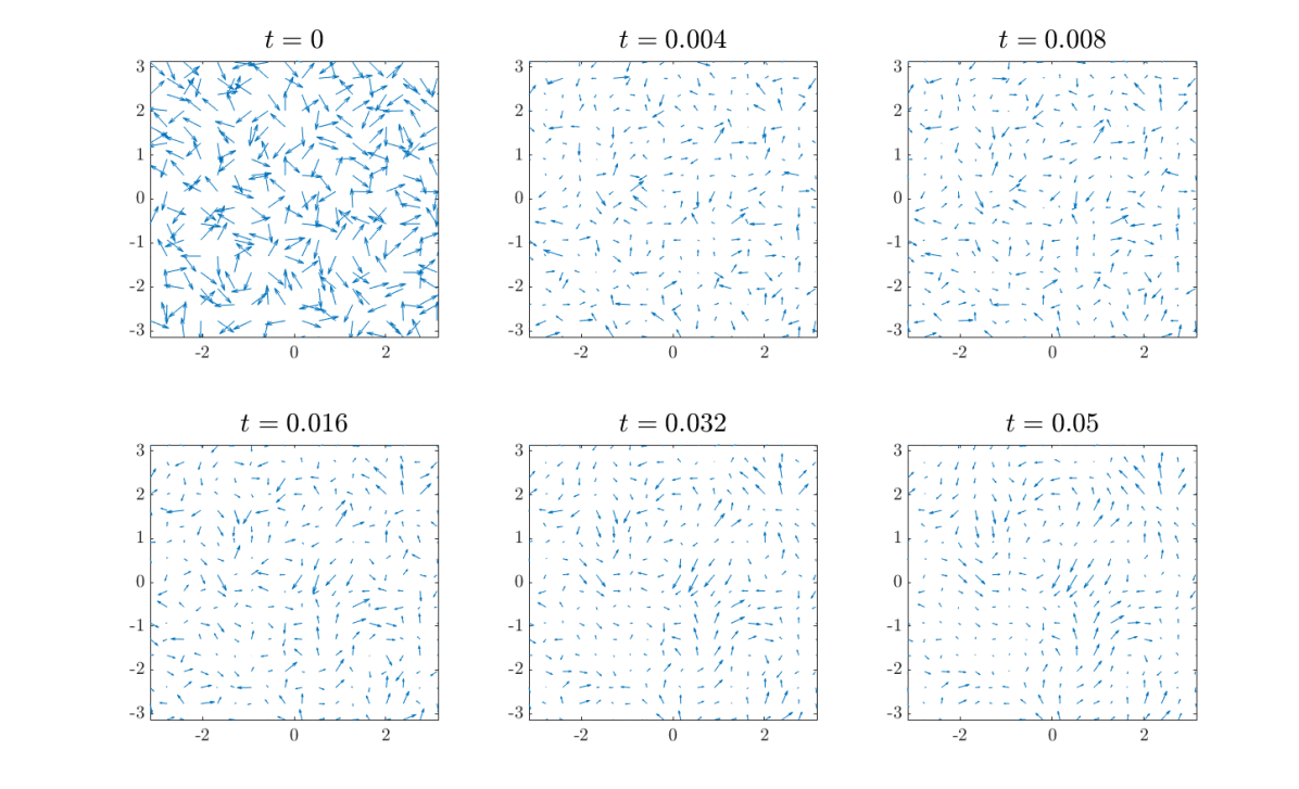
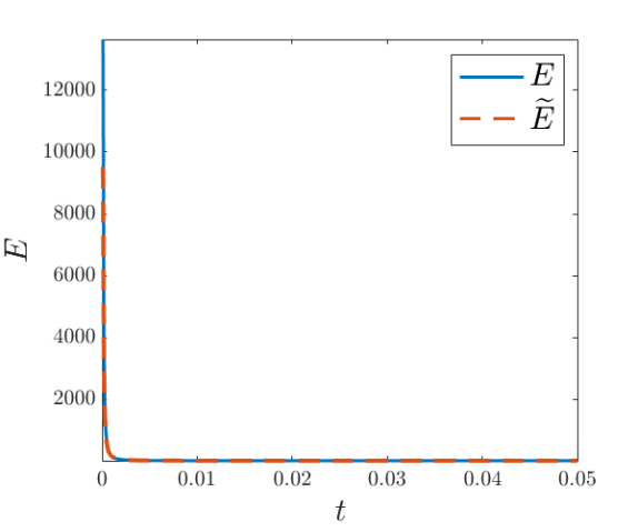
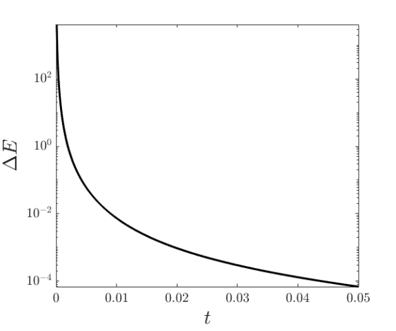
Figure 1. Vector field $\mathbf{u}$ at $t=0,~{}0.004,~{}0.008,~{}0.016,~{}0.032,$ and $0.05$ respectively for the vector-valued AC equation.

Figure 2. Evolution of the original and modified energy as well as their difference $\Delta E=|\widetilde{E}-E|$ for the vector-valued AC equation.

We now test the convergence order of the Strang splitting method for vector-valued Allen-Cahn equation with the same settings as above. Since the exact PDE solution is not available, we take a small splitting step $\tau=10^{-6}$ to obtain an “almost exact” solution at $t=0.01$. Then, we take several different splitting steps $\tau=\frac{1}{100}\times 2^{-k}$ with $k=5,6,\ldots,10$ to obtain corresponding numerical solutions at $t=0.01$. The $\ell_{2}$-errors between these solutions and the “almost exact” solution are summarized in Table 1. It can be observed that the convergence rate is about $2$.

Table 1. $\ell_{2}$-errors of numerical solutions at time $t=0.01$ to the vector-valued AC equation (4.1) for different splitting steps computed by the Strang splitting method.

  $\tau$ $\frac{1}{3200}$ $\frac{1}{6400}$ $\frac{1}{12800}$ $\frac{1}{25600}$ $\frac{1}{51200}$ $\frac{1}{102400}$ $\ell_{2}$-error $3.298\times 10^{-6}$ $1.199\times 10^{-6}$ $3.384\times 10^{-7}$ $8.932\times 10^{-8}$ $2.277\times 10^{-8}$ $5.684\times 10^{-9}$ rate – $1.4604$ $1.8245$ $1.9218$ $1.9716$ $2.0024$  

4.2. Matrix-valued AC equation

Consider the matrix-valued AC equation

$$\begin{cases}\partial_{t}U=\Delta U+U-UU^{\mathrm{T}}U,\quad(t,\mathbf{x})\in(0,\infty)\times\Omega;\\ U\Bigr{|}_{t=0}=U^{0}.\end{cases}$$ (4.6)

The spatial domain $\Omega=[-\pi,\,\pi]^{2}$ is the $2\pi$-periodic torus in dimension two. By a slight abuse of notation, we set the initial condition in polar coordinates as

$$U^{0}(r,\theta)=\left\{\begin{aligned} &\left[\begin{array}[]{cc}\cos\alpha&-\sin\alpha\\ \sin\alpha&\cos\alpha\end{array}\right]&&\mbox{if }r<0.6\pi+0.12\pi\sin(6\theta);\\ &\left[\begin{array}[]{cc}\cos\alpha&\sin\alpha\\ \sin\alpha&-\cos\alpha\end{array}\right]&&\mbox{otherwise,}\end{aligned}\right.$$ (4.7)

Here $\alpha(x,y)=\frac{\pi}{2}\sin(x+y)$, and $(r,\theta)$ is the polar coordinate of $\mathbf{x}=(x,y)$. For spatial discretization we use the pseudo-spectral method with $256\times 256$ Fourier modes. The splitting time step is fixed as $\tau=0.01$. In Figure 4, the domain is colored by the sign of the determinant of $U$, that is,

yellow $$\mbox{if }\det(U(t,x,y))>0;$$ (4.8)

blue $$\mbox{if }\det(U(t,x,y))<0.$$

The vector field is generated by the first column vector of the matrix $U(t,x,y)$. Note that for $t=0$ this is just

$$\left(\begin{array}[]{c}\cos\alpha\\ \sin\alpha\end{array}\right).$$ (4.9)

It can be observed that the initial star-shaped line defect shrinks in time. The evolution of the standard and the modified energy as well as their difference $\Delta E=|\widetilde{E}-E|$ are plotted in Figure 4. Clearly these two energy functionals are in good agreement for small $\tau>0$.

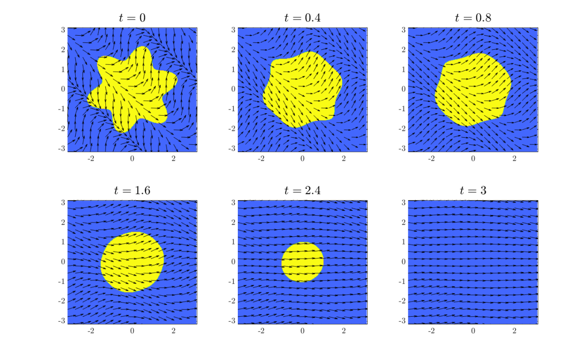
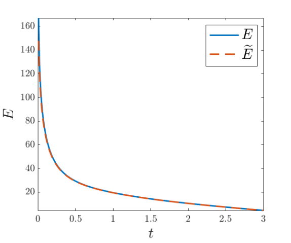
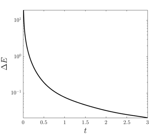
Figure 3. Dynamics of line defect for the matrix-valued AC equation at $t=0,~{}0.4,~{}0.8,~{}1.6,~{}2.4,$ and $3$ respectively with initial condition (4.7) in Section 4.2.

Figure 4. Evolution of the original and modified energy as well as their difference $\Delta E=|\widetilde{E}-E|$ for the matrix-valued AC equation with initial condition (4.7) in Section 4.2.

Next, we consider the initial condition given by the following.

$$U^{0}(r,\theta)=\left\{\begin{aligned} &\left[\begin{array}[]{cc}\cos\alpha&-\sin\alpha\\ \sin\alpha&\cos\alpha\end{array}\right]&&\mbox{if }|x|>0.5\pi|\sin(1.25y)|+0.4\pi,\\ &\left[\begin{array}[]{cc}\cos\alpha&\sin\alpha\\ \sin\alpha&-\cos\alpha\end{array}\right]&&\mbox{otherwise,}\end{aligned}\right.$$ (4.10)

where $\alpha=y$. The splitting time step is $\tau=0.01$ and we take $256\times 256$ Fourier modes. The dynamics of the line defect and the evolution of the energy are illustrated in Figure 6 and 6 respectively. It can be observed that the modified energy dissipation indeed holds in this case.

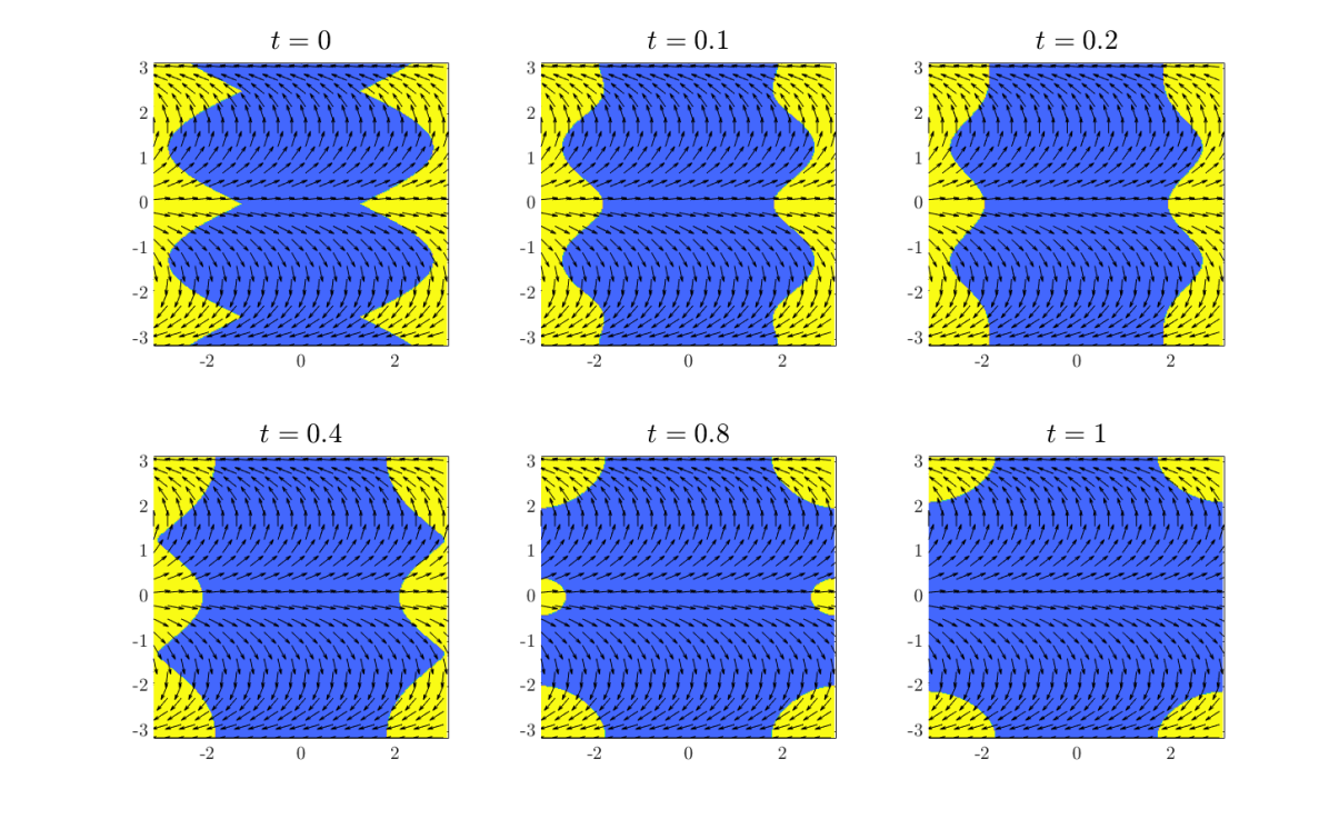
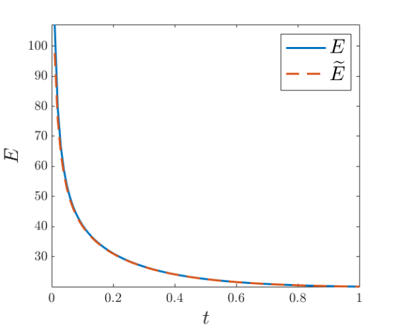
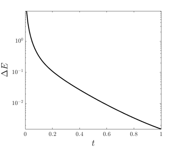
Figure 5. Dynamics of line defect for the matrix-valued AC equation at $t=0,~{}0.1,~{}0.2,~{}0.4,~{}0.8,$ and $1$ respectively with initial condition (4.10) in Section 4.2.

Figure 6. Evolution of the original and modified energy as well as their difference $\Delta E=|\widetilde{E}-E|$ for the matrix-valued AC equation with initial condition (4.10) in Section 4.2.

References

- [1] T. Batard and M.Bertalmio. On covariant derivatives and their applications to image regularization. SIAM Journal on Imaging Sciences 7, no. 4: 2393-2422, 2014.
- [2] Y. Cheng, A. Kurganov, Z. Qu, and T. Tang. Fast and stable explicit operator splitting methods for phase-field models. Journal of Computational Physics, 303:45–65, 2015.
- [3] Z. Weng and L. Tang. Analysis of the operator splitting scheme for the Allen-Cahn equation. Numerical Heat Transfer, Part B: Fundamentals, 70(5):472–483, 2016.
- [4] W. Bao, S. Jin, and P. A Markowich. On time-splitting spectral approximations for the Schrödinger equation in the semiclassical regime. Journal of Computational Physics, 175(2):487–524, 2002.
- [5] M. Thalhammer. Convergence analysis of high-order time-splitting pseudospectral methods for nonlinear Schrödinger equations. SIAM Journal on Numerical Analysis, 50(6):3231–3258, 2012.
- [6] S. Descombes. Convergence of a splitting method of high order for reaction-diffusion systems. Mathematics of Computation, 70(236):1481–1501, 2001.
- [7] A. Jaffe and C. Taube. Vortices and Monopoles: Structure of Static Gauge Theories. Birkhauser, Boston.
- [8] Elliott, C. M., Hiroshi Matano, and Tang Qi. Zeros of a complex Ginzburg–Landau order parameter with applications to superconductivity. European Journal of Applied Mathematics 5, no. 4 (1994): 431-448.
- [9] S. Zhao, J. Ovadia, X. Liu, Y. Zhang, and Q. Nie. Operator splitting implicit integration factor methods for stiff reaction–diffusion–advection systems. Journal of Computational Physics, 230(15):5996–6009, 2011.
- [10] G. Strang. On the construction and comparison of difference schemes. SIAM Journal on Numerical Analysis, 5(3):506–517, 1968.
- [11] G. I Marchuk. Splitting and alternating direction methods. Handbook of Numerical Analysis, 1:197–462, 1990.
- [12] Y. Li, H. G. Lee, D. Jeong, and J. Kim. An unconditionally stable hybrid numerical method for solving the Allen–Cahn equation. Computers & Mathematics with Applications, 60(6):1591–1606, 2010.
- [13] D. Li and C. Quan. The operator-splitting method for Cahn-Hilliard is stable. arXiv:2107.01418, 2021.
- [14] D. Li and C. Quan. On the energy stability of Strang-splitting for Cahn-Hilliard. arXiv:2107.05349, 2021.
- [15] D. Li and C. Quan. Negative time splitting is stable. arXiv:2107.07332, 2021.
- [16] D. Li, C. Quan, and T. Tang. Energy dissipation of Strang splitting method for Allen–Cahn equations. arXiv:2108.05214, 2021.
- [17] D. Li. Effective Maximum Principles for Spectral Methods. Ann. Appl. Math., 37 (2021), pp. 131–290.
- [18] B. Osting and D. Wang. A diffusion generated method for orthogonal matrix-valued fields. Mathematics of Computation, 89(322):515–550, 2020.
- [19] A. S Lewis and H. S Sendov. Nonsmooth analysis of singular values. Part I: Theory. Set-Valued Analysis, 13(3):213–241, 2005.
- [20] B. Li and Y. Wu. A fully discrete low-regularity integrator for the 1D periodic cubic nonlinear Schrödinger equation. Numer. Math. (to appear), arXiv:2101.03728
- [21] M. Fei, F. Lin, W. Wang, and Z. Zhang. Matrix-valued Allen-Cahn equation and the Keller-Rubinstein-Sternberg problem. arXiv:2106.08293, 2021.