Quantitative Predictions for $f(R)$ Gravity Primordial Gravitational Waves

Abstract

In this work we shall develop a quantitative approach for extracting predictions on the primordial gravitational waves energy spectrum for $f(R)$ gravity. We shall consider two distinct models which yield different phenomenology, one pure $f(R)$ gravity model and one Chern-Simons corrected potential-less $k$-essence $f(R)$ gravity model in the presence of radiation and non-relativistic perfect matter fluids. The two $f(R)$ gravity models were carefully chosen in order for them to describe in a unified way inflation and the dark energy era, in both cases viable and compatible with the latest Planck data. Also both models mimic the $\Lambda$-Cold-Dark-Matter model and specifically the pure $f(R)$ model only at late times, but the Chern-Simons $k$-essence model during the whole evolution of the model up to the radiation domination era. In addition they guarantee a smooth transition from the inflationary era to the radiation, matter domination and subsequently to the dark energy era. Using a WKB approach introduced in the relevant literature by Nishizawa, we derive formulas depending on the redshift that yield the modified gravity effect, quantified by a multiplicative factor, a “damping” in front of the General Relativistic waveform. In order to calculate the effect of the modified gravity, which is the “damping” factor, we solve numerically the Friedmann equations using appropriate initial conditions and by introducing specific statefinder quantities. As we show, the pure $f(R)$ gravity gravitational wave energy spectrum is slightly enhanced, but it remains well below the sensitivity curves of future gravitational waves experiments. In contrast, the Chern-Simons $k$-essence $f(R)$ gravity model gravitational wave energy spectrum is significantly enhanced and two signals are predicted which can be verified by future gravitational wave experiments. We discuss in detail our findings and the future perspective of modified gravity theories in view of the upcoming second and third generation experiments on primordial gravitational waves.

I Introduction

Inflation [1, 2, 3, 4] is to date the most promising candidate theory for describing the post-Planckian epoch of our Universe. The inflationary era is speculated to have occurred after the quantum gravity era of our Universe, and from the beginning of the inflationary era the Universe is assumed to be four dimensional and to be described by classical physics. The inflationary scenario is appealing since most inflationary theories generate a nearly scale invariant power spectrum of the primordial scalar perturbations, and it solves the most unappealing issues of standard Big Bang cosmology, such as the horizon and flatness problems. However, to date, the direct verification that inflation has ever occurred has not been accomplished yet. This direct verification of the inflationary era can be given only via the detection of the $B$-modes (curl modes) of inflation in the Cosmic Microwave Background (CMB) radiation temperature and polarization anisotropies [5]. The CMB probes modes with wavenumbers $k<0.62$ Mpc^-1, and for modes with wavenumbers larger than this cutoff it is impossible for the CMB to probe them, because for $f>0.15\times 10^{-15}$Hz the scalar perturbations are highly non-linear, thus CMB probes scales with wavelength $\lambda$ from $10$ Mpc to $10^{4}$ Mpc. $B$-mode polarization can mainly arise from two sources in the Universe, firstly from the primordial tensor perturbations, the inflationary tensor modes, which occur at the low-multipoles ($\ell\leq 10$) or equivalently large angular scales of the CMB radiation, or from the gravitational lensing conversion of the $E$-mode polarization modes into the (curl) $B$-modes, and this physical process occurs at late times and on small angular scales [6]. Thus, the goal of the next generation of CMB experiments has become the detection of CMB polarization patterns induced by inflationary tensor modes with wavelengths from $10$ Mpc to $10^{4}$ Mpc. It is conceivable that the CMB probes modes entered the horizon well after the Big Bang Nucleosynthesis (BBN) epoch which occurred for temperatures $T\sim 1$MeV with wavenumber $k_{BBN}=6.5\times 10^{3}$ Mpc^-1. Thus in some sense, the CMB offers insights for the physics that occurred during the last stages of the matter domination era, beyond the matter-radiation equality $k_{eq}\sim 0.05\,h^{2}$ Mpc^-1, leaving the physics of the early matter and radiation-reheating era untouched. The main reason for this is the fact that scalar perturbations become non-linear for wavelengths below $10$ Mpc. The modes with wavelength well below $10$ Mpc have entered the horizon well before the matter-radiation equality era, and these correspond to primordial tensor modes that probe the radiation and reheating era [5, 6, 7, 8, 9, 10, 11, 12, 13, 14, 15, 16, 17, 18, 19, 20, 21, 22, 23, 24, 25, 26, 27, 28, 29, 30, 31, 32, 33, 34, 35, 36, 37, 38, 39, 40, 41, 42, 43, 44, 45, 46, 47]. These inflationary modes have reentered the Hubble horizon after the end of the inflationary era first and this occurred during the reheating and radiation era. For these eras we basically know nothing and the only way to probe these eras is via the primordial gravitational waves. These inflationary waves form a stochastic background of inflationary tensor modes and carry important information about the conditions and state of our Universe during and after the inflationary era. The stochastic gravitational background is also strongly affected by the evolution of the Universe and is also affected by the matter content of our Universe after inflation. These effects imprinted on the stochastic gravitational wave background radiation offer incredible insights for the reheating and radiation domination eras and specifically between the end of inflation and the electroweak phase transition. The appealing feature of the stochastic gravitational wave background is that the primordial gravity waves have tiny amplitude and their interaction with matter is significantly small, which makes them obey linear evolution equations. Hence, their evolution is easier to predict, in contrast to density perturbations which are non-linear for modes larger than $10$ Mpc and grow at superhorizon scales. The primordial tensor modes are mainly affected by the first horizon crossing during inflation, also by the horizon reentry after inflation, and by the evolution itself of the Universe and of the matter content of the Universe. Indirectly, the effects of a modified gravity governing the evolution are imprinted also on primordial gravitational waves, since a modified gravity may directly affect the inflationary and post-inflationary era. Thus via the stochastic primordial gravitational waves background, which are nothing else but the superadiabatic amplified zero point fluctuations of the gravitational field, the physics of the post-inflationary early Universe might be uniquely probed and studied. If we will be able to probe these primordial tensor modes, we will be able to lay hands on cosmological eras which are currently unknown for us. Also let us note that the lowest frequency mode observable today corresponds to modes that have entered the Hubble horizon at present day, and these modes can be probed by the CMB. Basically, it is useful to understand the spectrum of frequencies existing in our Universe today. As we already mentioned, the lowest frequency mode probed by the CMB is the mode that enters the horizon today, and the maximum frequency of the primordial gravitational waves spectrum is $f_{max}\sim 1$GHz [18]. The physics in the range $f_{BBN}<f<f_{max}$ is pretty much unknown thus the primordial gravitational waves actually reveal information related to several features of this physically unknown era, not up to $f_{max}$ but for frequencies up to several Hz. The maximum frequency is hard to probe, but future experiments related to radiation and reheating era modes, will probe frequencies up to several hundreds of Hz.

The future experiments, second and third generation experiments, that will be able to probe modes that entered the Hubble horizon at temperatures much higher than the BBN one, are: ground-based interferometers, like the Einstein Telescope probing Hz-KHz frequencies [48], space-born interferometers like the LISA laser interferometer space antenna [49, 50], future space missions like the BBO (Big Bang Observer) [51, 52], the DECIGO [53, 54] and also the SKA (Square Kilometer Array) which will receive data from pulsar timing arrays at frequencies $10^{-8}$Hz [55]. Also currently and in the future the NANOGrav [56, 57] provides data on pulsar timing arrays too.

The future experiments like the BBO, DECIGO and LISA and the Einstein Telescope will probe frequencies that peak near the frequency range $f\sim\mathcal{O}(10^{-4}-1)$Hz, which basically corresponds to tensor modes with $k\sim\mathcal{O}(10^{10}-10^{15})$ Mpc^-1. These modes correspond to modes that have reentered the Hubble horizon well before the matter-radiation equality which in turn corresponds to modes with $k_{eq}\sim 0.05\,h^{2}$ Mpc^-1. Also the aforementioned future missions and experiments probe modes well beyond the tensor modes that have reentered the Hubble horizon during the BBN era, at $T\sim 1$MeV with wavenumber $k_{BBN}=6.5\times 10^{3}$ Mpc^-1. The maximum frequency of the primordial gravitational waves spectrum is $f_{max}\sim 1$GHz [18]. We need to note that the gravitational waves below $f\sim 10^{-15}$Hz are affected by a second order term of the scalar primordial perturbations, via the anisotropic stress term, and these effects cause a damping of the energy spectrum, but these frequencies are not of interest for future experiments which probe much higher frequencies.

The standard theory that is most frequently used for inflationary theories is the scalar field theory approach [1, 2, 3, 4]. However the scalar field description offers a very restricted description of inflation, which can also be connected with theoretical shortcomings like the Swampland issue [58, 59, 60, 61]. In addition, in the context of scalar field inflation it is usually quite difficult to describe in a unified way inflation and the dark energy era. In contrast, in the context of modified gravity in its various forms [62, 63, 64, 65, 66, 67], the unified description of inflation and the dark energy era can be accomplished, see for example the pioneer work in the context of $f(R)$ gravity [68] and for later developments see [69, 70, 71, 72, 73, 74, 75, 76, 77]. With regard to primordial gravitational waves, it seems that scalar field theories remain beyond the reach of future experiments, since the scalar field theory primordial gravitational wave energy spectrum lies well below the sensitivity curves of most of the future experiments [78]. In fact, the source of this problem seems to be the red-tilted tensor spectral index predicted by the scalar field theories. To date it is becoming a fact that a blue-tilted tensor spectral index will generate a gravitational wave energy spectrum that may be detected in the future second and third generation experiments on gravitational waves [25, 21]. In scalar field theory inflation, a blue-tilted tensor spectral index cannot be generated by a non-tachyonic theory [20], a factor that narrows the possibility of detection of scalar field theory inflation if indeed it describes inflation, if the latter ever occurred. Thus if inflation occurred primordially, and a signal of stochastic tensor perturbation is observed in the future experiments, single scalar field inflationary theory will be overruled from being a viable description of inflation. To this end modified gravity combined or not with scalar fields may provide a viable candidate theory for describing inflation. Motivated by this aspect, in this work we will study primordial gravitational waves in the context of $f(R)$ gravity. After providing some essential information about the General Relativistic (GR) waveform of the stochastic gravitational waves, we shall employ a WKB approach introduced by Nishizawa [27] in order to provide a quantifiable way to measure the effects of modified gravity on the primordial gravitational wave waveform. The resulting waveform contains the GR waveform multiplied by a “damping” factor, which is solely affected by the modified gravity controlling the evolution. This “damping” factor might actually cause an overall damping of the gravitational wave energy spectrum or might enhance it, depending on the underlying modified gravity controlling the evolution. The only way to calculate this “damping” factor is by solving the Friedmann equation numerically for the physically relevant redshift range, which extends from present day up to the radiation domination era. We shall introduce suitable statefinder quantities, dark energy based, and we shall transform the Friedmann equations appropriately in order to express them in terms of these statefinders and in terms of the redshift. Our aim is to study two distinct $f(R)$-gravity related models, firstly a pure $f(R)$ gravity model and secondly a Chern-Simons potential-less $k$-essence $f(R)$ gravity, both in the presence of dark matter and radiation perfect fluids. For the pure $f(R)$ gravity case, the contribution of the modified gravity on the ‘damping” term basically is absent beyond redshift $z\sim 1000$, and also for redshifts for which the total equation of state (EoS) parameter reaches the radiation domination value $\omega_{tot}\sim 1/3$, the “damping” term is zero. Thus we provide a calculation of the “damping” factor and the result is that the actual pure $f(R)$ gravitational wave spectrum is slightly enhanced compared to the GR one, but still remains well below the sensitivity curves of the future experiments. The possibility of having enhanced gravitational wave spectrum in the context of $f(R)$ gravity has also been stressed in Refs. [44, 45, 46]. We perform the same analysis for the Chern-Simons $k$-essence $f(R)$ gravity, and as we will show, the primordial gravitational wave energy spectrum is significantly enhanced, and can be detectable by most of the future experiments. More importantly, we show that due to the Chern-Simons term, the prediction for the theory is actually not one, but two distinct signals peaking at the same frequency range. Also we demonstrate that the reheating temperature significantly affects the gravitational wave energy spectrum. Thus by using two appropriate toy models, we show in a quantitative way what may occur in future experiments. For both the models we considered, we used models that may describe the dark energy and the inflationary era within the same theoretical framework, so the models we used are severely constrained phenomenologically. Moreover as a side remark, the models we used were actually able to also describe the intermediate eras in between the inflationary and the dark energy era, that is, the matter and radiation domination eras, and a smooth transition between all cosmological eras. Also one of the models behaves exactly as the $\Lambda$-Cold-Dark-Matter ($\Lambda$CDM) model. We also discuss the future observations outcomes, in view of our findings and we theorize what a detection or a non-detection of a signal would mean for inflationary physics.

This work is organized as follows: In section II we present the essential features of the primordial gravitational waves in the context of GR and we also present how to apply the WKB method in order to extract the modified gravity effects on the primordial gravitational waves waveform. We consider two cases, the pure $f(R)$ gravity case and a Chern-Simons corrected $k$-essence $f(R)$ gravity, and we provide explicit formulas in both cases for the “damping” factor and the primordial gravitational wave energy spectrum. In the same section we describe in brief our strategy for obtaining the “damping” factor and we discuss our aim to present two models that can describe inflation and dark energy in a unified way. In section III we shall study two distinct models of $f(R)$ gravity with respect to the primordial gravitational wave energy spectrum, firstly a pure $f(R)$ gravity model and secondly a Chern-Simons $k$-essence $f(R)$ gravity model, both in the presence of dark matter and radiation perfect fluids. In both cases the models were appropriately chosen in order for them to provide a unified description of inflation and the dark energy eras. We provide for both the models detailed description for the dark energy era, and beyond, by solving numerically the Friedmann equation using appropriate initial conditions, and we also discuss the inflationary aspects of the models. Accordingly we calculate for both models the “damping” factor and the overall effect of modified gravity on the primordial gravitational wave energy spectrum. We also provide detailed predictions for the produced gravitational wave energy spectrum and we compare our findings with the projected sensitivities of the most future experiments, for a wide range of frequencies. We also discuss in some detail what implications for inflation would have the absence or presence of a signal in future experiments. Finally, the concluding remarks along with a critical discussion on our findings are presented in the conclusions section.

II Primordial Gravitational Waves in Einstein-Hilbert and $f(R)$ Gravity

II.1 The Einstein-Hilbert Gravity Case

Before getting to the core of this work, it is vital to present some general features of primordial gravitational waves in the context of standard general relativity (GR) and in the context of $f(R)$ gravity. We shall adopt the notation and conventions of Refs. [8, 27, 28, 30, 19, 20] and references therein. The material that will be presented is not new but it will help the article to be self-contained.

Let us start with the GR description of inflationary gravitational waves. For our analysis we shall assume a spatially flat Friedmann-Robertson-Walker (FRW) metric with line element,

$$\centering{\rm d}s^{2}=-{\rm d}t^{2}+a(t)^{2}\sum_{i=1}^{3}{({\rm d}x^{i})^{2}}\,,\@add@centering$$ (1)

where $a(t)$ denotes the scale factor and $t$ denotes the cosmic time. For inflationary gravitational waves considerations, it is usually more convenient to use the conformal time $\tau$, in which case the line element of the FRW spacetime reads,

$${\rm d}s^{2}=a^{2}[-{\rm d}\tau^{2}+(\delta_{ij}+h_{ij}){\rm d}x^{i}{\rm d}x^{j}],$$ (2)

and $x^{i}$ denotes the comoving spatial coordinates, while $h_{ij}$ stands for the gauge-invariant metric tensor perturbation. The metric tensor perturbation $h_{ij}$ is symmetric ($h_{ij}\!=\!h_{ji}$), and satisfies the traceless $h_{ii}\!=\!0$, and transverse $\partial^{j}h_{ij}\!=\!0$ conditions. Treating the tensor perturbation $h_{ij}(\tau,{\bf x})$ as a quantum field embedded in an unperturbed FRW spacetime $g_{\mu\nu}=diag\{-a^{2},a^{2},a^{2},a^{2}\}$, and by keeping order two terms in $h_{ij}$ in the Lagrangian of the gravitational field, the tensor perturbations quadratic action is given by,

$$S=\int d\tau d{\bf x}\sqrt{-g}\left[\frac{-g^{\mu\nu}}{64\pi G}\partial_{\mu}h_{ij}\partial_{\nu}h_{ij}+\frac{1}{2}\Pi_{ij}h_{ij}\right].$$ (3)

with $g^{\mu\nu}$ being the inverse of $g_{\mu\nu}$ and $g$ denoting its determinant. The anisotropic stress $\Pi_{\mu\nu}$, with its tensor part being,

$$\Pi^{i}_{j}=T^{i}_{j}-p\delta^{i}_{j}$$ (4)

satisfies $\Pi_{ii}=0$ and the transverse condition $\partial^{i}\Pi_{ij}=0$, and its coupling to the tensor perturbation $h_{ij}$ acts like an external source in the gravitational quantum action (3). Upon variation of the action (3) with respect to the tensor perturbation $h_{ij}$, we get the following equation of motion,

$$h_{ij}^{\prime\prime}+2\frac{a^{\prime}(\tau)}{a(\tau)}h_{ij}^{\prime}-{\bf\nabla}^{2}h_{ij}=16\pi Ga^{2}(\tau)\Pi_{ij}(\tau,{\bf x}),$$ (5)

where the prime denotes differentiation with respect to the conformal time $\tau$. Performing a Fourier transform in the equation of motion (5), we obtain,

$$h_{ij}(\tau,{\bf x})\!\! =\! \!\!\sum_{r}\sqrt{16\pi G}\!\!\int\!\!\!\frac{d{\bf k}}{(2\pi)^{3/2}}\epsilon_{ij}^{r}({\bf k})h_{{\bf k}}^{r}(\tau){\rm e}^{i{\bf k}{\bf x}},\qquad\quad$$ (6a)

$$\Pi_{ij}(\tau,{\bf x})\!\! =\! \!\!\sum_{r}\sqrt{16\pi G}\!\!\int\!\!\!\frac{d{\bf k}}{(2\pi)^{3/2}}\epsilon_{ij}^{r}({\bf k})\Pi_{{\bf k}}^{r}(\tau){\rm e}^{i{\bf k}{\bf x}},\qquad\quad$$ (6b)

where $r=$(“$+$” or “$\times$”) indicates the polarization of the gravitational tensor perturbation. We need to note that the Fourier transform is essential in order to obtain the evolution equation corresponding to each mode quantified by the wavenumber $\vec{k}$. Also, Eq. (5) describes the evolution of the metric tensor perturbation, which depends on space and time, but for the analysis of the primordial gravitational waves, it is required to obtain the behavior of each mode of specific frequency and wavenumber $\vec{k}$. Each Fourier mode has only time dependence, thus it’s evolution can be split in several distinct evolutionary eras, plus the subhorizon and superhorizon behavior can easily be obtained.

Also the polarization tensors satisfy [$\epsilon_{ij}^{r}({\bf k})=\epsilon_{ji}^{r}({\bf k})$], and also satisfy the traceless $\epsilon_{ii}^{r}({\bf k})=0$, and the transverse conditions $k_{i}\epsilon_{ij}^{r}({\bf k})=0$, as it is expected. By choosing a circular-polarization basis in which $\epsilon_{ij}^{r}({\bf k})=(\epsilon_{ij}^{r}(\textrm{-}{\bf k}))^{\ast}$, we can normalize the polarization basis in the following way,

$$\sum_{i,j}\epsilon_{ij}^{r}({\bf k})(\epsilon_{ij}^{s}({\bf k}))^{\ast}=2\delta^{rs}.$$ (7)

Combining Eq. (6) and (3), we obtain,

$$S\!=\!\!\sum_{r}\!\!\int\!\!d\tau d{\bf k}\frac{a^{2}}{2}\;\!\!\Big{[}h_{{\bf k}}^{r}{}^{\prime}h_{\!\textrm{-}{\bf k}}^{r}\!{}^{\prime}\!-\!k^{2}h_{{\bf k}}^{r}h_{\!\textrm{-}{\bf k}}^{r}\!+\!32\pi Ga^{2}\Pi_{{\bf k}}^{r}h_{\!\textrm{-}{\bf k}}^{r}\Big{]}\,,$$ (8)

so essentially we obtain the original action of the tensor perturbations (3) expressed in terms of the Fourier transformed tensor perturbations. This is essential for the quantization of the resulting action (6), in order to impose the isochronous commutation relations for each distinct wavenumbers $\vec{k}$ and $\vec{k}^{\prime}$. These relations are much more simplified in Fourier space and can easily result to the well-known quantum algebra for the bosonic creation and annihilation operators. So we can proceed to the canonical quantization of the above action, with $h_{{\bf k}}^{r}$ being the canonical variable and its conjugate momentum being

$$\pi_{{\bf k}}^{r}(\tau)=a^{2}(\tau)h_{\!\textrm{-}{\bf k}}^{r}{}^{\prime}(\tau)\,,$$ (9)

so by promoting these variables to quantum operators $\hat{h}_{{\bf k}}^{r}$ and $\hat{\pi}_{{\bf k}}^{r}$, we can quantize the theory by imposing the equal-time commutation relations,

$$\left[\hat{h}_{{\bf k}}^{r}(\tau),\hat{\pi}_{{\bf k}^{\prime}}^{s}(\tau)\right] = i\delta^{rs}\delta^{(3)}({\bf k}-{\bf k}^{\prime}),$$ (10a)

$$\left[\hat{h}_{{\bf k}}^{r}(\tau),\hat{h}_{{\bf k}^{\prime}}^{s}(\tau)\right] = \left[\hat{\pi}_{{\bf k}}^{r}(\tau),\hat{\pi}_{{\bf k}^{\prime}}^{s}(\tau)\right]=0.$$ (10b)

Note that the Fourier components of $\hat{h}_{ij}(\tau,{\bf x})$ satisfy $\hat{h}_{{\bf k}}^{r}=\hat{h}_{\!\textrm{-}{\bf k}}^{r{\dagger}}$, due to the fact that $\hat{h}_{ij}(\tau,{\bf x})$ is Hermitian. Accordingly we can write these as follows,

$$\hat{h}_{{\bf k}}^{r}(\tau)=h_{k}(\tau)\hat{a}_{{\bf k}}^{r}+h_{k}^{\ast}(\tau)\hat{a}_{\!\textrm{-}{\bf k}}^{r{\dagger}},$$ (11)

with the $\hat{a}_{{\bf k}}^{r{\dagger}}$ being the creation operators and $\hat{a}_{{\bf k}}^{r}$ being the annihilation operators, which satisfy the standard commutation relations,

$$\Big{[}\hat{a}_{{\bf k}}^{r},\hat{a}_{{\bf k}^{\prime}}^{s{\dagger}}\Big{]} = \delta^{rs}\delta^{(3)}({\bf k}-{\bf k}^{\prime}),$$ (12a)

$$\Big{[}\hat{a}_{{\bf k}}^{r},\hat{a}_{{\bf k}^{\prime}}^{s}\Big{]} = \Big{[}\hat{a}_{{\bf k}}^{r{\dagger}},\hat{a}_{{\bf k}^{\prime}}^{s{\dagger}}\Big{]}=0\,.$$ (12b)

Also the linearly-independent modes $h_{k}(\tau)$ and $h_{k}^{\ast}(\tau)$ are solutions of the Fourier transformed equation of motion,

$$h_{k}^{\prime\prime}+2\frac{a^{\prime}(\tau)}{a(\tau)}h_{k}^{\prime}+k^{2}h_{k}=16\pi Ga^{2}(\tau)\Pi_{k}(\tau).$$ (13)

From Eq. (11) it is apparent that the modes $h_{k}(\tau)$ depend on the conformal time and on the wavenumber $k=|{\bf k}|$, and not on the polarization and the direction. The compatibility constraint between the two commutation relations (10) and (12), is basically the following Wronskian normalization condition,

$$h_{k}(\tau)h_{k}^{\ast}{}^{\prime}(\tau)-h_{k}^{\ast}(\tau)h_{k}^{\prime}(\tau)=\frac{i}{a^{2}(\tau)}$$ (14)

in the chronological past. The initial condition chosen in the literature in the chronological past is the Bunch-Davies vacuum,

$$h_{k}(\tau)\to\frac{{\rm exp}(-ik\tau)}{a(\tau)\sqrt{2k}}\qquad({\rm as}\;\;\tau\to-\infty),$$ (15)

which describes the modes $\vec{k}$ which are still in subhorizon scales during inflation, and of course satisfies relation (14). For the quantitative study of the stochastic primordial gravitational wave background, we shall use two frequently used in the literature spectra, the tensor power spectrum $\Delta_{h}^{2}(k,\tau)$ and the energy spectrum of primordial gravitational waves $\Omega_{gw}(k,\tau)$. We have,

$$\langle 0|\hat{h}_{ij}(\tau,{\bf x})\hat{h}_{ij}(\tau,{\bf x})|0\rangle\!=\!\!\!\int_{0}^{\infty}\!\!\!\!\!64\pi G\frac{k^{3}}{2\pi^{2}}\!\left|h_{k}(\tau)\right|^{2}\!\frac{dk}{k},$$ (16)

and therefore, the inflationary tensor power spectrum is,

$$\Delta_{h}^{2}(k,\tau)\equiv\frac{d\langle 0|\hat{h}_{ij}^{2}|0\rangle}{d\,{\rm ln}\,k}=64\pi G\frac{k^{3}}{2\pi^{2}}\left|h_{k}(\tau)\right|^{2}.$$ (17)

The present day energy spectrum of the stochastic primordial gravitational waves background $\Omega_{gw}(k,\tau)$ is given by,

$$\Omega_{gw}(k,\tau)\equiv\frac{1}{\rho_{crit}(\tau)}\frac{d\langle 0|\hat{\rho}_{gw}(\tau)|0\rangle}{d\,{\rm ln}\,k}$$ (18)

and it basically corresponds to the gravitational-wave energy density ($\rho_{gw}$) calculated per logarithmic wavenumber interval, and the critical energy density is given by,

$$\rho_{crit}(\tau)=\frac{3H^{2}(\tau)}{8\pi G}.$$ (19)

In order to calculate $\Omega_{gw}(k,\tau)$, we can assume that the tensor perturbation $h_{ij}$ is a quantum field in the unperturbed FRW background, and by using its action (3), we can calculate its stress-energy tensor, which is,

$$T_{\alpha\beta}=-2\frac{\delta L}{\delta\bar{g}^{\alpha\beta}}+\bar{g}_{\alpha\beta}L,$$ (20)

where $L$ stands for the Lagrangian function in (3). Therefore, the gravitational wave energy density in the absence of anisotropic stress couplings (this simplification is justified for frequencies larger than the CMB frequencies) is,

$$\rho_{gw}=-T_{0}^{0}=\frac{1}{64\pi G}\frac{(h_{ij}^{\prime})^{2}+(\vec{{\bf\nabla}}h_{ij})^{2}}{a^{2}},$$ (21)

with its vacuum expectation value being,

$$\langle 0|\rho_{gw}|0\rangle=\int_{0}^{\infty}\frac{k^{3}}{2\pi^{2}}\frac{\left|h_{k}^{\prime}\right|^{2}+k^{2}\left|h_{k}\right|^{2}}{a^{2}}\frac{dk}{k},$$ (22)

and therefore the stochastic gravitational wave energy spectrum is given by,

$$\Omega_{gw}(k,\tau)=\frac{8\pi G}{3H^{2}(\tau)}\frac{k^{3}}{2\pi^{2}}\frac{\left|h_{k}^{\prime}(\tau)\right|^{2}+k^{2}\left|h_{k}(\tau)\right|^{2}}{a^{2}(\tau)}.$$ (23)

Furthermore, by using $|h_{k}^{\prime}(\tau)|^{2}=k^{2}|h_{k}(\tau)|^{2}$, we may write the gravitational wave energy spectrum at present day as,

$$\Omega_{gw}(k,\tau)=\frac{1}{12}\frac{k^{2}\Delta_{h}^{2}(k,\tau)}{H_{0}^{2}(\tau)}\,.$$ (24)

where we assumed that the scale factor at present day is $a_{0}=1$ and $H_{0}$ stands for the present day Hubble rate, which is $H_{0}\sim 67.3$ according to the latest Planck CMB based constraints. There is a tension between the CMB-based value of $H_{0}$ and the one indicated by the Cepheids, however in the present paper we shall take into account only the CMB-based value for the current Hubble rate, until several issues related to the calibration of data for the Cepheids observations are consistently and firmly resolved [79, 80]. Once the mode with comoving wave number $k$ becomes superhorizon evolving, the amplitude of the gravitational wave remains constant and when it reenters the horizon, the amplitude is dumped. In the present work we shall consider modes that became subhorizon at some point after inflation, during the mysterious reheating and radiation era.

The amplitude of the gravitational wave with comoving wave number $k$ remains constant when the mode lies outside the horizon. However, once it entered the horizon, its amplitude begins to damp. Regarding the mode which re-enters the Hubble horizon during the matter-dominated era, we have [8, 27, 28, 30, 19, 20],

$$h_{k}^{\lambda}(\tau)=h_{k}^{\lambda({\rm p})}\left(\frac{3j_{1}(k\tau)}{k\tau}\right),$$ (25)

with $j_{\ell}$ denoting the $\ell$-th spherical Bessel function. The Fourier-transformed tensor perturbation solution during a cosmological era for which the Hubble rate evolves as a power-law one, namely, $a(t)\propto t^{p}$, takes the form,

$$h_{k}(\tau)\propto a(t)^{\frac{1-3p}{2p}}J_{\frac{3p-1}{2(1-p)}}(k\tau),$$ (26)

where $J_{n}(x)$ is the Bessel function. Another damping effect for the $h_{k}(\tau)$ must be taken into account, having to do with the fact that in the early Universe, the relativistic degrees of freedom do not remain constant and the scale factor behaves as $a(t)\propto T^{-1}$ [22], so the damping factor is,

$$\left(\frac{g_{*}(T_{\rm in})}{g_{*0}}\right)\left(\frac{g_{*s0}}{g_{*s}(T_{\rm in})}\right)^{4/3},$$ (27)

with $T_{\rm in}$ denoting the horizon re-entry temperature, which is,

$$T_{\rm in}\simeq 5.8\times 10^{6}~{}{\rm GeV}\left(\frac{g_{*s}(T_{\rm in})}{106.75}\right)^{-1/6}\left(\frac{k}{10^{14}~{}{\rm Mpc^{-1}}}\right).$$ (28)

Furthermore, another damping factor is due to the current acceleration of the Universe $\sim(\Omega_{m}/\Omega_{\Lambda})^{2}$ [8]. In the literature, the present day gravitational wave energy spectrum per log frequency interval contains the above damping effects, and also two transfer factors that result from the numerical integration of the Fourier transformed differential equation governing the evolution of the tensor perturbations, so that the final expression is,

$$\Omega_{\rm gw}(f)=\frac{k^{2}}{12H_{0}^{2}}\Delta_{h}^{2}(k),$$ (29)

with $\Delta_{h}^{2}(k)$ being equal to [8, 27, 28, 30, 19, 20],

$$\Delta_{h}^{2}(k)=\Delta_{h}^{({\rm p})}(k)^{2}\left(\frac{\Omega_{m}}{\Omega_{\Lambda}}\right)^{2}\left(\frac{g_{*}(T_{\rm in})}{g_{*0}}\right)\left(\frac{g_{*s0}}{g_{*s}(T_{\rm in})}\right)^{4/3}\left(\overline{\frac{3j_{1}(k\tau_{0})}{k\tau_{0}}}\right)^{2}T_{1}^{2}\left(x_{\rm eq}\right)T_{2}^{2}\left(x_{R}\right)\,,$$ (30)

and the “bar” in the Bessel function term, denoting the average over many periods. The term $\Delta_{h}^{({\rm p})}(k)^{2}$ stands for the primordial tensor power spectrum related to the inflationary era, which is [8, 27, 28, 30, 19, 20],

$$\Delta_{h}^{({\rm p})}(k)^{2}=\mathcal{A}_{T}(k_{ref})\left(\frac{k}{k_{ref}}\right)^{n_{T}}\,,$$ (31)

and it is evaluated at the CMB pivot scale $k_{ref}=0.002$ Mpc^-1, and $n_{T}$ is the inflationary tensor spectral index. Here, $\mathcal{A}_{T}(k_{ref})$ is the amplitude of the tensor perturbations primordially, which is related to the amplitude of the scalar perturbations $\mathcal{P}_{\zeta}(k_{ref})$ and the tensor-to-scalar ratio as follows,

$$\mathcal{A}_{T}(k_{ref})=r\mathcal{P}_{\zeta}(k_{ref})\,,$$ (32)

therefore the primordial tensor spectrum is finally written as follows,

$$\Delta_{h}^{({\rm p})}(k)^{2}=r\mathcal{P}_{\zeta}(k_{ref})\left(\frac{k}{k_{ref}}\right)^{n_{T}}\,.$$ (33)

Now, the transfer function $T_{1}(x_{\rm eq})$ in Eq. (30) connects basically the gravitational wave spectrum of a mode $k$ which re-entered the horizon near the matter-radiation equality, $t=t_{\rm eq}$ and it is given by [8, 27, 28, 30, 19, 20],

$$T_{1}^{2}(x_{\rm eq})=\left[1+1.57x_{\rm eq}+3.42x_{\rm eq}^{2}\right],$$ (34)

with $x_{\rm eq}=k/k_{\rm eq}$ and $k_{\rm eq}\equiv a(t_{\rm eq})H(t_{\rm eq})=7.1\times 10^{-2}\Omega_{m}h^{2}$ Mpc^-1. Also the transfer function $T_{2}(x_{R})$ in Eq. (30) characterizes modes that re-entered the horizon after the reheating era commenced but before it ended, so for $k>k_{R}$, and it reads,

$$T_{2}^{2}\left(x_{R}\right)=\left(1-0.22x^{1.5}+0.65x^{2}\right)^{-1}\,,$$ (35)

with $x_{R}=\frac{k}{k_{R}}$, and the $k_{R}$ wavenumber is,

$$k_{R}\simeq 1.7\times 10^{13}~{}{\rm Mpc^{-1}}\left(\frac{g_{*s}(T_{R})}{106.75}\right)^{1/6}\left(\frac{T_{R}}{10^{6}~{}{\rm GeV}}\right)\,,$$ (36)

where $T_{R}$ is the reheating temperature, and this temperature will be a free variable in our paper, since it may affect the present day energy spectrum of the gravitational waves. The corresponding reheating frequency is,

$$f_{R}\simeq 0.026~{}{\rm Hz}\left(\frac{g_{*s}(T_{R})}{106.75}\right)^{1/6}\left(\frac{T_{R}}{10^{6}~{}{\rm GeV}}\right),$$ (37)

and note that the reheating frequency $f_{R}$ is quite close to the most sensitive frequency band of DECIGO and BBO for $T_{R}\sim 10^{7}~{}{\rm GeV}$. Of course as we already mentioned, the reheating temperature is a variable in our theory, and basically its scale is still a mystery that refers to the hypothetical reheating era. Finally, let us quote an expression for $g_{*}(T_{\mathrm{in}}(k))$ appearing in Eq. (30) [15],

$$g_{*}(T_{\mathrm{in}}(k))=g_{*0}\left(\frac{A+\tanh\left[-2.5\log_{10}\left(\frac{k/2\pi}{2.5\times 10^{-12}\mathrm{Hz}}\right)\right]}{A+1}\right)\left(\frac{B+\tanh\left[-2\log_{10}\left(\frac{k/2\pi}{6\times 10^{-19}\mathrm{Hz}}\right)\right]}{B+1}\right)\,,$$ (38)

where $A$ and $B$ are,

$$A=\frac{-1-10.75/g_{*0}}{-1+10.75g_{*0}}\,,$$ (39)

$$B=\frac{-1-g_{max}/10.75}{-1+g_{max}/10.75}\,,$$ (40)

where $g_{max}=106.75$ and $g_{*0}=3.36$. The same formulas as above, namely Eqs. (38), (39) and (40), can be used for calculating $g_{*0}(T_{\mathrm{in}}(k))$ by replacing $g_{*0}=3.36$ with $g_{*s}=3.91$.

II.2 Primordial Gravity Waves in $f(R)$ Gravity: A WKB Approach

Let us consider the following perturbation of a flat FRW spacetime,

$${\rm d}s^{2}=-a(\tau)^{2}{\rm d}\tau^{2}-2a(\tau)^{2}\beta_{,i}{\rm d}\tau{\rm d}x^{i}+a(\tau)^{2}\left(g_{ij}^{(3)}+2\varphi g_{ij}^{(3)}+2\gamma_{,i|j}+2h_{ij}\right){\rm d}x^{i}{\rm d}x^{j}\,,$$ (41)

with $i,j=1,2,3$, and the above perturbation includes both tensor and scalar type perturbations, with the former being denoted as $h_{ij}$ and it is traceless, symmetric and transverse, that is $h_{ii}=0$, $h_{\alpha\beta}=h_{\beta\alpha}$ and $\partial^{j}h_{ij}=0$ respectively. Also the scalar type perturbations are quantified by the functions $\beta$, $\gamma$ and $\varphi$, and the spatial part of the FRW metric $g_{ij}^{(3)}$ is,

$$g_{ij}^{(3)}{\rm d}x^{i}{\rm d}x^{j}={\rm d}r^{2}+r^{2}\left({\rm d}\theta^{2}+\sin^{2}\theta{\rm d}\phi^{2}\right)\,.$$ (42)

We shall consider two types of Lagrangian densities, and here we shall quote two expressions for the differential equation that governs the evolution of tensor type perturbations. Firstly, consider a pure $f(R)$ gravity action of the form,

$$\mathcal{S}=\int{\rm d}^{4}x\sqrt{-g}\left(\frac{f(R)}{2\kappa^{2}}+\mathcal{L}_{m}\right)\,,$$ (43)

where $\mathcal{L}_{m}$ denotes the Lagrangian density of the matter perfect fluids that are present. The differential equation that governs the evolution of the tensor perturbation $C_{ij}$ is the following [81],

$$\frac{1}{a^{3}f_{R}}\frac{{\rm}d}{{\rm d}t}\left(a^{3}f_{R}\dot{h}_{ij}\right)-\frac{\nabla^{2}}{a^{2}}h_{ij}=0\,,$$ (44)

where $\nabla^{2}$ is the Laplacian corresponding to the three dimensional spacelike hypersurface spatial part of the FRW spacetime, and $f_{R}=\frac{\partial f}{\partial R}$. Also we ignored anisotropic stress effects, due to the fact that we are interested in large frequencies, and anisotropic stress effects are strong below $\mathcal{O}(10^{-16})$Hz, so at CMB frequencies only. If we consider the Fourier transformation of the tensor perturbation $h_{ij}$ given in Eq. (6), the evolution equation (44) for both polarizations becomes,

$$\frac{1}{a^{3}f_{R}}\frac{{\rm}d}{{\rm d}t}\left(a^{3}f_{R}\dot{h}(k)\right)+\frac{k^{2}}{a^{2}}h(k)=0\,,$$ (45)

which can be rewritten as follows,

$$\ddot{h}(k)+\left(3+\alpha_{M}\right)H\dot{h}(k)+\frac{k^{2}}{a^{2}}h(k)=0\,,$$ (46)

where $\alpha_{M}$ for the $f(R)$ gravity case at hand is,

$$a_{M}=\frac{f_{RR}\dot{R}}{f_{R}H}\,.$$ (47)

Note that the evolution differential equation (46) is valid for both the polarization modes and in effect there is no inequivalent propagation between these two modes. This is not however true in the presence of a non-trivial Chern-Simons term as we show shortly. The evolution equation (46) is almost identical with the one derived in Ref. [27, 28, 29], apart from a typo perhaps in the second term (and of course in Ref. [27, 28, 30] the conformal time is used), and it is identical with the one appearing in [30]. Refs. [27, 28, 29, 30] considered the more general class of Horndeski theories, but we specified the study in $f(R)$ gravity for clarity and transparency of the following sections. Now the study of the evolution of primordial gravitational waves can be simplified by adopting Nishizawa’s approach [27, 28], which is a WKB-based method. Let us analyze it in brief, in order to have available the formulas needed for the sections to follow. First, let us transform the evolution equation in the conformal time equivalent, which is,

$$h^{\prime\prime}(k)+\left(2+a_{M}\right)\mathcal{H}h^{\prime}(k)+k^{2}h(k)=0\,,$$ (48)

where the prime indicates differentiation with respect to the conformal time $\tau$ and $\mathcal{H}=\frac{a^{\prime}}{a}$. Now using Nishizawa’s WKB approach, the WKB solution to the differential equation (48) is of the form,

$$h=e^{-\mathcal{D}}h_{GR}\,,$$ (49)

where $h_{GR}$ is the GR waveform solution corresponding to the differential equation (48) with $a_{M}=0$ and also $\mathcal{D}$ has the following form,

$$\mathcal{D}=\frac{1}{2}\int^{\tau}a_{M}\mathcal{H}{\rm d}\tau_{1}=\frac{1}{2}\int_{0}^{z}\frac{a_{M}}{1+z^{\prime}}{\rm dz^{\prime}}\,,$$ (50)

where we expressed finally $\mathcal{D}$ as an integral over the redshift. Note that in the case of $f(R)$ gravity, the gravitational wave speed is equal to unity, thus an extra damping term present in Nishizawa’s paper is absent in our case. Thus in order to find the primordial gravitational waveform in the case of $f(R)$ gravity, one has to calculate the “damping” factor $\mathcal{D}$ up to a redshift corresponding to the era suitable for the observations of LISA, BBO, DECIGO etc. which correspond to quite large frequencies and to modes that reentered the Hubble horizon quite close to the reheating era. Also the “damping” term $e^{-\mathcal{D}}$ might not eventually be an actual damping term since it is possible that this term might lead to an amplification of the gravitational wave energy spectrum, due to the specific form of the $f(R)$ gravity. This feature is more or less model dependent, but our results indicate that most viable $f(R)$ gravities indeed lead to damping effects, apart from the models that we will present in this paper.

We need to note that Nishizawa’s WKB solution is basically valid only for modes that are subhorizon during present day and the modes that reentered the Hubble horizon during the beginning of the radiation era and during the mysterious reheating era, are basically subhorizon modes. Let us express $a_{M}$ as a function of the redshift, and we easily find that,

$$a_{M}=-\frac{f_{RR}}{f_{R}}(1+z)\frac{{\rm d}R(z)}{{\rm d}z}\,,$$ (51)

and basically in order to calculate the total “damping” (or amplification factor, but we shall quote it damping factor hereafter for convenience) factor we must integrate numerically the Friedmann equation for $f(R)$ gravity up to a redshift that corresponds to the era at which the modes of interest reentered the Hubble horizon and became subhorizon modes. These modes became subhorizon modes during the reheating era, definitely during the radiation domination era, so the redshift is at least of the order of $z\sim\mathcal{O}(10^{6})$. In order to have a precise idea on how large redshifts one must use in order to consistently calculate the damping factor, recall that the redshift and the Universe’s temperature are related as follows [82],

$$T=T_{0}(1+z)\,,$$ (52)

where $T_{0}$ is the present day temperature. Thus considering temperatures corresponding to the reheating era, which are of the GeV order, and also by taking into account that the present day Universe’s temperature is 3 Kelvin, or $T_{0}=2.58651\times 10^{-4}$eV, then for temperatures of the GeV order, one obtains $z\sim 3.86621\times 10^{12}$ or larger. It is apparent that integrating the Friedmann equation at such large redshifts might be a formidable task, however, things can get much easier by recalling that when the total EoS of the Universe $\omega_{tot}$ becomes of the order of $\omega_{tot}\sim 1/3$, the scale factor evolves as $a(t)\sim t^{1/2}$, and therefore $\dot{R}$ is identically zero, and the same applies for the Ricci scalar $R$. Thus, if the term $f_{RR}/f_{R}$ does not become singular for $R=0$ and behaves as a constant, then the parameter $a_{M}$ in Eq. (47) becomes equal to zero. Therefore it is not necessary to calculate the integral (50) for redshifts larger than the ones for which $\omega_{tot}\sim 1/3$. This feature greatly simplifies the calculations, since for redshifts larger than the ones for which $\omega_{tot}\sim 1/3$, the damping factor $e^{-\mathcal{D}}$ becomes unity, and the GR waveform describes perfectly the gravitational wave (30).

II.3 Primordial Gravity Waves in Chern-Simons $k$-essence $f(R)$ Gravity: A WKB Approach

Apart from the pure $f(R)$ gravity models, another interesting class of modified gravity models, that leads to particularly interesting phenomenological predictions, is Chern-Simons corrected $k$-essence $f(R)$ gravity. The reason we chose this specific modified gravity to study it along with the pure $f(R)$ gravity is mainly the fact that it leads to a unique prediction for the primordial gravitational wave energy spectrum: the predicted signal has two components, thus two signals are predicted and more importantly the GR signal is significantly amplified for frequencies probed by the LISA mission, or even higher. Consider again the perturbation of the FRW metric appearing in Eq. (41) and now the underlying theory is assumed to be a Chern-Simons corrected $k$-essence $f(R)$ gravity, in which case the general action is,

$$\mathcal{S}=\int{\rm d}^{4}x\sqrt{-g}\left(\frac{f(R,X,\phi)}{2}+\mathcal{L}_{m}+\frac{1}{8}\nu(\phi)\eta^{abcd}R_{ab}^{\ \ ef}R_{cdef}\right)\,,$$ (53)

where again $\mathcal{L}_{m}$ denotes the Lagrangian density of the matter perfect fluids that are present and $\eta^{abcd}$ is a totally antisymmetric Levi-Civita tensor density. Also $X$ in the action above is the kinetic term $X=\frac{1}{2}\partial^{\mu}\phi\partial_{\mu}\phi$. The action (53) describes the Chern-Simons corrected $f(R,X,\phi)$ theory with the Chern-Simons coupling being $\nu(\phi)$. In the end, we shall specify the $f(R,X,\phi)$ theory to be a potential-less $k$-essence $f(R)$ gravity. The Chern-Simons term affects solely the tensor perturbations evolution, and does not affect at all the scalar perturbations and the field equations for a FRW spacetime. In effect, the Chern-Simons term affects the inflationary era via the tensor-to-scalar ratio and the tensor spectral index, and indirectly it will affect the energy spectrum of the primordial gravitational waves via the primordial scaling $\sim k^{n_{T}}$. For the action (53), the evolution differential equation that governs the tensor perturbation is [81],

$$\frac{1}{a^{3}}\frac{d}{dt}\left(a^{3}\dot{h}_{\alpha\beta}\right)-\frac{\nabla^{2}}{\alpha^{2}}h_{\alpha\beta}-\frac{2\kappa^{2}}{a}\epsilon_{(\alpha}^{\ \ \mu\nu}\left((\ddot{\nu}-H\dot{\nu})\dot{h}_{\beta)\mu}+\dot{\nu}D_{\beta)\mu}\right)_{,\nu}=0\,,$$ (54)

with $D_{\alpha\beta}=\ddot{h}_{\alpha\beta}+3H\dot{h}_{\alpha\beta}-\frac{\nabla^{2}}{a^{2}}h_{\alpha\beta}$. This evolution equation describes the tensor mode evolution, however it is not diagonal, thus by making the following Fourier transformation,

$$\centering h_{\alpha\beta}=\sqrt{Vol}\int{\frac{d^{3}k}{(2\pi)^{3}}\sum_{\ell}\epsilon_{\alpha\beta}^{(\ell)}(\vec{k})h_{\ell\vec{k}}e^{i\vec{k}\vec{x}}}\,,\@add@centering$$ (55)

Eq. (54) is diagonalized in the following way,

$$\centering\frac{1}{a^{3}Q_{t}}\frac{d}{dt}\left(a^{3}Q_{t}\dot{h}_{\ell\vec{k}}\right)+\frac{k^{2}}{a^{2}}h_{\ell\vec{k}}=0\,,\@add@centering$$ (56)

where,

$$Q_{t}=f_{R}+2\lambda_{\ell}\dot{\nu}\frac{k}{a}$$ (57)

and $f_{R}=\frac{\partial f(R,X,\phi)}{\partial R}$. In the case at hand, $h_{\ell\vec{k}}$ describes a tensor mode perturbation with polarization $l$, and $\epsilon_{\alpha\beta}^{(\ell)}$ denotes the circular polarization tensor which has the property $ik_{\gamma}\varepsilon_{\alpha}^{\gamma\delta}\epsilon^{(\ell)}_{\beta\delta}=k\lambda_{\ell}\epsilon^{(\ell)}_{\alpha\beta}$. Apparently the evolution equation (56) describes the distinct evolution of two polarization modes, the left-handed ($\lambda_{L}=-1$) and right handed modes ($\lambda_{R}=1$). The presence of parameter $Q_{t}$ directly makes the propagation of the left and right handed modes inequivalent. For the $f(R,X,\phi)$ theory at hand, the propagation speed of the tensor perturbations is equal to unity in natural units, thus it is equal to the light speed, however, the wave speed of the scalar perturbations is not equal to unity, but this will concern us when we deal with the inflationary aspects of the current theory. For the moment let us focus on the tensor perturbations, so the evolution equation for a polarization $\ell$ can be written as follows,

$$\ddot{h}(k)+\left(3+\alpha_{M\ell}\right)H\dot{h}(k)+\frac{k^{2}}{a^{2}}h(k)=0\,,$$ (58)

where $\alpha_{M}$ for the $f(R,X,\phi)$ gravity case at hand is equal to,

$$a_{M\ell}=\frac{\dot{Q}_{t}}{Q_{t}H}\,,$$ (59)

and by using the definition of $Q_{t}$ given in (57), the parameter $a_{M}$ becomes,

$$a_{M\ell}=\frac{f_{RR}\dot{R}+2\lambda_{\ell}\ddot{\nu}k/a-2\lambda_{\ell}\dot{\nu}kH/a}{(f_{R}+2\lambda_{\ell}\dot{\nu}k/a)}\,,$$ (60)

and note that we basically have two parameters $a_{M\ell}$, one corresponding to the left handed and one to the right handed polarization. The above expression can easily be expressed in terms of the redshift, and the primordial gravitational wave form for the theory at is again given by Eq. (50). Thus again by integrating the corresponding Friedmann equation up to a certain redshift, we may obtain the “damping” factor $\mathcal{D}$ in Eq. (50). The new feature is that the theory predicts basically two distinct signals of primordial gravitational waves, corresponding to the left and right handed polarizations which propagate in an inequivalent way. Also let us again note that the expression for $a_{M\ell}$ is simplified for redshifts which correspond to the radiation domination era with $\omega_{tot}\sim 1/3$, and acquires the following form,

$$a_{M\ell}=\frac{2\lambda_{\ell}\ddot{\nu}k/a-2\lambda_{\ell}\dot{\nu}kH/a}{(f_{R}+2\lambda_{\ell}\dot{\nu}k/a)}\,.$$ (61)

II.4 Strategy for Obtaining the Precise “Damping” Caused by Modified Gravity Effects and Constraints

Let us analyze in brief in this section the strategy and the aims of the sections that follow. Our aim is to make exact predictions for the primordial gravitational wave energy spectrum for some $f(R)$ gravity models of particular interest. The $f(R)$ gravity models are not randomly selected, but these satisfy quite stringent viability criteria, with respect to their early and late-time phenomenology. We shall consider one pure $f(R)$ gravity model and one Chern-Simons corrected $k$-essence $f(R)$ gravity model without scalar potential. Both these models produce a successful inflationary era, compatible with the latest Planck constraints on inflation [83], and we shall extract the tensor-to-scalar ratio and the tensor spectral index for both the models, since these two observational parameters are essential for the calculation of the primordial gravitational wave energy spectrum. Furthermore, the models predict a viable dark energy era, with predictions that are compatible with the latest Planck constraints on the cosmological parameters [84]. Apparently, both the models provide a theoretical framework for which the inflationary era and the dark energy era can be described in a unified way, thus the two models were chosen by taking into account stringent criteria. Now with regard to the predictions for the primordial gravitational wave energy spectrum, our aim in both models is to calculate the damping factor $e^{-\mathcal{D}}$, so this amounts in calculating the integral of Eq. (50), namely $\mathcal{D}=\frac{1}{2}\int_{0}^{z}\frac{a_{M}}{1+z^{\prime}}{\rm dz^{\prime}}$, from zero redshift, which corresponds to present time, until a high redshift corresponding to the modes that reentered the Hubble horizon during the radiation domination era, and specifically during the pretty much unknown reheating epoch. Most of the proposed experiments, such as the LISA mission, BBO, DECIGO, Einstein Telescope and so on, probe frequencies that correspond to wavelengths of modes that reentered the Hubble horizon during the reheating epoch, so this justifies why considering such extremely large redshifts. Thus our central goal is to calculate the integral of Eq. (50) for both models with two distinct damping effects on the primordial gravitational waves energy spectrum, quantified by the parameters $a_{M}$ appearing in Eq. (47) for the pure $f(R)$ gravity model, and by the parameter $a_{M\ell}$ appearing in Eq. (59) for the Chern-Simons corrected $k$-essence $f(R)$ gravity model. In order to calculate the integral numerically, one must know the Hubble rate $H(z)$ for both models, so in order to find this, we will solve numerically the Friedmann equation for both models. To this end, we shall introduce some statefinder variable quantities, expressed in terms of the Hubble rate, and we shall rewrite the Friedmann equations for both models in terms of this new statefinder quantities, using the redshift as a dynamical variable, instead of the cosmic time. By solving numerically the Friedmann equation, and having an interpolating numerical solution for the Hubble rate, facilitates very much the calculation of the damping factor for both models. A cumbersome issue is the choice of the final redshift, since the reheating era corresponds to significantly high redshifts. For the pure $f(R)$ gravity case things are easy, since as we will show, the integral beyond redshifts of the order $z\sim\mathcal{O}(4\times 10^{5})$ is essentially zero due to its highly oscillating behavior. Apart from this model dependent feature, in the pure $f(R)$ gravity case, when the total EoS parameter is approximately $\omega_{tot}\sim 1/3$, the cosmological model is described by a radiation domination era scale factor, thus $R=0$ and $\dot{R}=0$, hence for the model we shall consider, for which $\frac{f_{RR}}{f_{R}}\neq 0$ for $R=0$, the parameter $a_{M}$ is identically zero during the radiation domination era. This feature can be used for future studies of pure $f(R)$ gravity models by the readers. Also for the case of the Chern-Simons corrected $k$-essence $f(R)$ gravity model, we shall integrate the Friedmann equation for maximum redshifts of the order $z\sim\mathcal{10^{5}}$, since beyond that the total EoS parameter becomes approximately $\omega_{tot}\sim 1/3$ and it proves numerically that the integral for both left and right polarization modes is nearly zero. After calculating the exact damping for both models, we plot the $h^{2}$-scaled gravitational wave energy spectrum versus the frequency by using the $h_{GR}$ waveform with the damping factor we calculated, and we make exact predictions for the spectrum, comparing it with the sensitivity curves of the most interesting future experiments.

Finally, let us bear in mind that there are upper constraints for the gravitational wave energy spectrum, coming from various sources, and it is worth quoting these here. Firstly, at low multipoles of CMB and at low frequencies, of the order $f\sim\mathcal{O}(10^{-17})\,$Hz, the gravitational wave spectrum is constrained to be $h^{2}\Omega_{GW}\sim 10^{-16}$ [14], at $f\sim\mathcal{O}(3\times 10^{-16})\,$Hz, the gravitational wave spectrum is constrained to be $h^{2}\Omega_{GW}<8.4\times 10^{-7}$ [14] (without taking into account anisotropic stress effects) and for $3\times 10^{-16}{\rm Hz}<f<10^{-15}\,$Hz, the gravitational wave spectrum is constrained to be $h^{2}\Omega_{GW}<8.6\times 10^{-7}$ (including anisotropic stress from neutrino free streaming) [14]. Also for $f\geq 10^{-15}\,$Hz, the gravitational wave spectrum is constrained to be $h^{2}\Omega_{GW}<1.7\times 10^{-6}$ for adiabatic initial conditions and $h^{2}\Omega_{GW}<2.9\times 10^{-7}$ for homogeneous initial conditions [14]. Also the Big Bang Nucleosynthesis bound is,

$$\Omega_{GW}h^{2}\leq\frac{n_{T}(2-n_{T})}{2}\times 5.6\times 10^{-6}(N_{ef}-3)\,,$$ (62)

with $N_{ef}=4.65$ (95$\%$CL) [15].

III Specific Models Predictions and Quantitative Analysis

III.1 Unified Description of Inflation and Dark Energy I: A Pure $f(R)$ Gravity Model

Let us first consider a pure $f(R)$ gravity model to check the gravitational wave spectrum in this case. We have chosen an $f(R)$ gravity model which allows the unified description of the inflationary era with the dark energy era. This model was discussed in some previous works, see for example [75, 76], so we refer the reader to these works for details. In this work we shall briefly discuss the model for completeness, and in the end we shall calculate numerically the “damping” factor for this model. Eventually we shall calculate the primordial gravitational wave energy density at present day, and we shall discuss the possibility of detection in this case. Consider the pure $f(R)$ gravity action in the presence of the perfect matter fluid Lagrangian $\mathcal{L}$, which we shall assume to be cold dark matter and radiation fluids,

$$\mathcal{S}=\int d^{4}x\sqrt{-g}\left[\frac{1}{2\kappa^{2}}f(R)+\mathcal{L}_{m}\right]\,,$$ (63)

where $\kappa^{2}=\frac{1}{8\pi G}=\frac{1}{M_{p}^{2}}$, and with $G$ being Newton’s gravitational constant while $M_{p}$ denotes the reduced Planck mass. The specific form of the $f(R)$ gravity that we will use in this work is,

$$f(R)=R+\frac{1}{M^{2}}R^{2}-\gamma\Lambda\Big{(}\frac{R}{3m_{s}^{2}}\Big{)}^{\delta}\,,$$ (64)

with $m_{s}$ in Eq. (64) being $m_{s}^{2}=\frac{\kappa^{2}\rho_{m}^{(0)}}{3}$, and $\rho_{m}^{(0)}$ being the energy density of cold dark matter today. Parameter $\delta$ is deliberately chosen to take values in the interval $0<\delta<1$, $\gamma$ is a freely chosen dimensionless parameter, and parameter $\Lambda$ is a free parameter with mass dimensions $[m]^{2}$. Furthermore, for phenomenological reasons [85], parameter $M$ is chosen to be $M=1.5\times 10^{-5}\left(\frac{N}{50}\right)^{-1}M_{p}$, where $N$ is number of $e$-foldings during inflation. For a flat FRW spacetime, upon varying the action (63) with respect to the metric, we get the following equations of motion,

$$3H^{2}f_{R}=\frac{Rf_{R}-f}{2}-3H\dot{f}_{R}+\kappa^{2}\left(\rho_{m}+\rho_{r}\right)\,,$$ (65)

$$-2\dot{H}f_{R}=\ddot{f}_{R}-H\dot{f}_{R}+\frac{4\kappa^{2}}{3}\rho_{r}\,,$$

where $f_{R}=\frac{\partial f}{\partial R}$ and the “dot” as usual denotes differentiation with respect to the cosmic time. Also $\rho_{r}$ and $\rho_{m}$ denote the radiation and cold dark matter energy densities respectively. The model (64) produces an inflationary era which is basically controlled by the $R^{2}$ model, as we now evince. Apparently the $\sim R^{\delta}$ term is subleading at early times, as we explicitly show now, and controls the late-time dynamics. For the model (64), the equations of motion (65) become,

$$3H^{2}\left(1+\frac{2}{M^{2}}R-\frac{\gamma\delta\Lambda}{(3m_{s}^{2})^{\delta}}R^{\delta-1}\right)=\frac{R^{2}}{2M}+\frac{\gamma(1-\delta)\Lambda}{2}\Big{(}\frac{R}{3m_{s}^{2}}\Big{)}^{\delta}-3H\dot{R}\Big{(}\frac{2}{M^{2}}-\frac{\gamma\delta(\delta-1)\Lambda}{(3m_{s}^{2})^{\delta}}R^{\delta-2}\Big{)}+\kappa^{2}\Big{(}\rho_{r}+\rho_{m}\Big{)}\,.$$ (66)

We shall assign the following values for the free dimensionless parameters $\gamma$ and $\delta$,

$$\gamma=\frac{1}{0.5},\,\,\,\delta=\frac{1}{100}\,,$$ (67)

and moreover let $\Lambda\simeq 11.895\times 10^{-67}$eV² which is chosen to take values almost identical with the present day cosmological constant. Also recall that $m_{s}^{2}\simeq 1.87101\times 10^{-67}$eV² and $M=1.5\times 10^{-5}\left(\frac{N}{50}\right)^{-1}M_{p}$ [85], so for $N\sim 60$, $M$ is $M\simeq 3.04375\times 10^{22}$eV. Assuming a slow-roll evolution during inflation, we have $R\simeq 12H^{2}$, so for a low-scale inflationary era, with $H=H_{I}\sim 10^{13}$GeV, the curvature scalar becomes approximately $R\sim 1.2\times 10^{45}$eV². Having these data at hand, we can proceed and directly compare the terms of Eq. (66),

For a low-scale inflationary era, with $H=H_{I}\sim 10^{13}$GeV, we have $R\sim 1.2\times\mathcal{O}(10^{45})$eV², $R^{2}/M^{2}\sim\mathcal{O}(1.55\times 10^{45})$eV² and also $\sim\Big{(}\frac{R}{3m_{s}^{2}}\Big{)}^{\delta}\sim\mathcal{O}(10)$. Moreover we have $\sim\Big{(}\frac{R}{3m_{s}^{2}}\Big{)}^{\delta-1}\sim\mathcal{O}(10^{-111})$ and lastly $\sim\Big{(}\frac{R}{3m_{s}^{2}}\Big{)}^{\delta-2}\sim\mathcal{O}(10^{-223})$. Therefore only the terms with positive powers of the curvature dominate the Friedmann equation (66), which becomes at leading order,

$$3H^{2}\left(1+\frac{2}{M^{2}}R\right)=\frac{R^{2}}{2M}-\frac{6H\dot{R}}{M^{2}}\,,$$ (68)

which is basically identical with the $R^{2}$ model case. Rewriting it we get,

$$3\ddot{H}-3\frac{\dot{H}^{2}}{H}+\frac{2M^{2}H}{6}=-9H\dot{H}\,,$$ (69)

and by solving it, assuming a slow-roll evolution we have,

$$H(t)=H_{0}-\frac{M^{2}}{36}t\,,$$ (70)

which is a quasi-de Sitter evolution that leads directly to the $R^{2}$ model spectral index and tensor-to-scalar ratio, which are,

$$n_{s}\sim 1-\frac{2}{N},\,\,\,r\sim\frac{12}{N^{2}}\,.$$ (71)

Also let us calculate in detail the tensor-spectral index for the $R^{2}$ model, which is essential for the calculation of the primordial gravitational wave energy spectrum. Recall the slow-roll indices for $f(R)$ gravity are [81, 62, 86],

$$\epsilon_{1}=-\frac{\dot{H}}{H^{2}},\quad\epsilon_{2}=0\,,\quad\epsilon_{3}=\frac{\dot{f}_{R}}{2Hf_{R}}\,,\quad\epsilon_{4}=\frac{\ddot{f}_{R}}{H\dot{f}_{R}}\,,$$ (72)

and from the Raychaudhuri equation for $f(R)$ gravity we have,

$$\epsilon_{1}=-\epsilon_{3}(1-\epsilon_{4})\,.$$ (73)

The tensor spectral index for $f(R)$ gravity is equal to [81, 62, 86],

$$n_{T}\simeq-2(\epsilon_{1}+\epsilon_{3})\,,$$ (74)

so in order to compute it for the $R^{2}$ gravity, we need an approximate expression for $\epsilon_{4}$. Let us focus on the slow-roll index $\epsilon_{4}$, and we easily find that,

$$\epsilon_{4}=\frac{\ddot{f}_{R}}{H\dot{f}_{R}}=\frac{\frac{d}{dt}\left(f_{RR}\dot{R}\right)}{Hf_{RR}\dot{R}}=\frac{f_{RRR}\dot{R}^{2}+f_{RR}\frac{d(\dot{R})}{dt}}{Hf_{RR}\dot{R}}\,.$$ (75)

However, $\dot{R}$ is equal to,

$$\dot{R}=24\dot{H}H+6\ddot{H}\simeq 24H\dot{H}=-24H^{3}\epsilon_{1}\,,$$ (76)

where the slow-roll approximation $\ddot{H}\ll H\dot{H}$ is used above and also we assumed in Eq. (76) that $\dot{R}\simeq 24H\dot{H}\simeq-24H^{3}\epsilon_{1}$, hence we avoided the appearance of the term $\sim\frac{d^{3}H}{dt^{2}}$ in the final expression. Combining Eqs. (76) and (75) after some algebra we get,

$$\epsilon_{4}\simeq-\frac{24f_{RRR}H^{2}}{f_{RR}}\epsilon_{1}-3\epsilon_{1}+\frac{\dot{\epsilon}_{1}}{H\epsilon_{1}}\,,$$ (77)

but $\dot{\epsilon}_{1}$ is explicitly equal to,

$$\dot{\epsilon}_{1}=-\frac{\ddot{H}H^{2}-2\dot{H}^{2}H}{H^{4}}=-\frac{\ddot{H}}{H^{2}}+\frac{2\dot{H}^{2}}{H^{3}}\simeq 2H\epsilon_{1}^{2}\,,$$ (78)

hence the final approximate expression for $\epsilon_{4}$ is,

$$\epsilon_{4}\simeq-\frac{24f_{RRR}H^{2}}{F_{RR}}\epsilon_{1}-\epsilon_{1}\,.$$ (79)

For the case of $R^{2}$ gravity obviously $\epsilon_{4}\simeq-\epsilon_{1}$, hence the tensor spectral index for the $R^{2}$ model reads,

$$n_{T}\simeq-2\frac{\epsilon_{1}^{2}}{1+\epsilon_{1}}\simeq-2\epsilon_{1}^{2}\,,$$ (80)

and due to the fact that $\epsilon_{1}\simeq\frac{1}{2N^{2}}$ for the $R^{2}$ model, the resulting expression for the tensor spectral index corresponding to the $R^{2}$ model is,

$$n_{T}\simeq-\frac{1}{2N^{2}}\,,$$ (81)

so for $N=60$ it is approximately $n_{T}=-0.000138889$ and it is always red-tilted of course. In the same vain, for $N=60$, the tensor-to-scalar ratio $r=12/N^{2}$ is equal to $r=0.00333333$ and we shall use both these values for the calculation of the gravitational wave energy spectrum. Having dealt with the early-time era essentials, let us proceed in finding a way to express the field equations in terms of appropriate statefinder variables and in terms of the redshift. This will make the integration needed for the calculation of the damping factor easier, since we shall basically numerically integrate the statefinder transformed equations of motion. First let us note that we can form the $f(R)$ gravity equations of motion to have the most familiar Einstein-Hilbert form as follows,

$$3H^{2}=\kappa^{2}\rho_{tot}\,,$$ (82)

$$-2\dot{H}=\kappa^{2}(\rho_{tot}+P_{tot})\,,$$

where $\rho_{tot}=\rho_{m}+\rho_{DE}+\rho_{r}$ denotes the total energy density of the cosmological fluid and $P_{tot}=P_{r}+P_{DE}$ denotes the total pressure. The total fluid has three components, the cold dark matter, the pressure and the geometric fluid, which at early times drives inflation, and at late times drives the dark energy era. The energy density of the geometric fluid reads,

$$\rho_{DE}=\frac{f_{R}R-f}{2}+3H^{2}(1-f_{R})-3H\dot{f}_{R}\,,$$ (83)

and its pressure reads,

$$P_{DE}=\ddot{f}_{R}-H\dot{f}_{R}+2\dot{H}(f_{R}-1)-\rho_{G}\,.$$ (84)

All the fluids considered are perfect fluids, and satisfy the following continuity equations,

$$\dot{\rho}_{m}+3H(\rho_{m}+P_{m})=0\,,$$ (85)

$$\dot{\rho}_{r}+3H(\rho_{r}+P_{r})=0\,,$$

$$\dot{\rho}_{DE}+3H(\rho_{DE}+P_{DE})=0\,.$$

Let us use the redshift $z$ as a dynamical variable, defined as follows,

$$1+z=\frac{1}{a}\,,$$ (86)

where the present day scale factor $a_{0}$, thus at $z=0$, is assumed to be unity for the simple reason that the physical and comoving wavenumbers at present time, $k$ and $a_{0}k$ coincide. We introduce the following statefinder quantity [87, 75, 76], follows,

$$y_{H}(z)=\frac{\rho_{G}}{\rho^{(0)}_{m}}\,,$$ (87)

where $\rho^{(0)}_{m}$ is the energy density of cold dark matter at present time. We can express the equations of motion in terms of the statefinder $y_{H}(z)$, by using the Friedmann equation, and we have,

$$y_{H}(z)=\frac{3H^{2}}{\kappa^{2}\rho^{(0)}_{m}}-\frac{\rho_{m}}{\rho^{(0)}_{m}}-\frac{\rho_{r}}{\rho^{(0)}_{m}}\,.$$ (88)

But $\rho_{r}$ redshifts as $\rho_{r}=\rho_{r}^{(0)}a^{-4}$, with $\rho_{r}^{(0)}$ being the value of the radiation energy density today, so $\frac{\rho_{r}}{\rho^{(0)}_{m}}=\chi(1+z)^{4}$, where $\chi=\frac{\rho^{(0)}_{r}}{\rho^{(0)}_{m}}\simeq 3.1\times 10^{-4}$. Also $\rho_{m}$ redshifts as $\rho_{m}=\rho_{m}^{(0)}a^{-3}$ thus, the function $y_{H}(z)$ of Eq. (88) can be written as follows,

$$y_{H}(z)=\frac{H^{2}}{m_{s}^{2}}-(1+z)^{3}-\chi(1+z)^{4}\,.$$ (89)

with $m_{s}^{2}=\frac{\kappa^{2}\rho^{(0)}_{m}}{3}=H_{0}\Omega_{c}=1.37201\times 10^{-67}$eV². By using the function $y_{H}(z)$ we can rewrite the cosmological equations of motion as one equation [87, 75, 76],

$$\frac{d^{2}y_{H}(z)}{dz^{2}}+J_{1}\frac{dy_{H}(z)}{dz}+J_{2}y_{H}(z)+J_{3}=0\,,$$ (90)

with the functions $J_{1}$, $J_{2}$ and $J_{3}$ being defined in the following way,

$$J_{1}=\frac{1}{z+1}\left(-3-\frac{1-f_{R}}{\left(y_{H}(z)+(z+1)^{3}+\chi(1+z)^{4}\right)6m_{s}^{2}f_{RR}}\right)\,,$$ (91)

$$J_{2}=\frac{1}{(z+1)^{2}}\left(\frac{2-f_{R}}{\left(y_{H}(z)+(z+1)^{3}+\chi(1+z)^{4}\right)3m_{s}^{2}f_{RR}}\right)\,,$$

$$J_{3}=-3(z+1)-\frac{\left(1-f_{R}\right)\Big{(}(z+1)^{3}+2\chi(1+z)^{4}\Big{)}+\frac{R-f}{3m_{s}^{2}}}{(1+z)^{2}\Big{(}y_{H}(z)+(1+z)^{3}+\chi(1+z)^{4}\Big{)}6m_{s}^{2}f_{RR}}\,,$$

with $f_{RR}=\frac{\partial^{2}f}{\partial R^{2}}$. The central point of our analysis is to solve numerically the above equation (90) by choosing suitable initial conditions, from redshift zero, up to a suitably high redshift that will be determined by the phenomenology of the model and the behavior of the parameter $a_{M}$ in Eq. (51). Then by finding the numerical solution $y_{H}(z)$, we can easily express all the necessary quantities needed for the calculation of $a_{M}$, as functions of $y_{H}(z)$. Particularly, the Ricci scalar is written in terms of $y_{H}(z)$ as follows,

$$R(z)=3m_{s}^{2}\left(4y_{H}(z)-(z+1)\frac{dy_{H}(z)}{dz}+(z+1)^{3}\right)\,.$$ (92)

Furthermore, the Hubble rate in terms of $y_{H}(z)$ is written as,

$$H_{\Lambda}(z)=H_{0}\sqrt{\Omega_{\Lambda}+\Omega_{M}(z+1)^{3}+\Omega_{r}(1+z)^{4}}\,,$$ (93)

where $H_{0}$ is the value of the Hubble rate today which is $H_{0}\simeq 1.37187\times 10^{-33}$eV based on the latest Planck data [84], also $\Omega_{\Lambda}\simeq 0.681369$ and $\Omega_{M}\sim 0.3153$ [84], while $\Omega_{r}/\Omega_{M}\simeq\chi$, and $\chi$ was defined earlier in this section. Moreover, the dark energy density parameter $\Omega_{DE}$ reads,

$$\Omega_{DE}(z)=\frac{y_{H}(z)}{y_{H}(z)+(z+1)^{3}+\chi(z+1)^{4}}\,,$$ (94)

and the dark energy EoS parameter reads,

$$\omega_{DE}(z)=-1+\frac{1}{3}(z+1)\frac{1}{y_{H}(z)}\frac{dy_{H}(z)}{dz}\,.$$ (95)

Finally, the deceleration parameter and the total EoS parameter as functions of the redshift and $y_{H}(z)$ read,

$$q=-1-\frac{\dot{H}}{H^{2}}=\frac{(z+1)H^{\prime}(z)}{H(z)}-1\,,$$ (96)

$$\omega_{tot}=-1-\frac{2\dot{H}}{3H^{2}}=-1+\frac{2(1+z)H^{\prime}(z)}{3H(z)}\,.$$ (97)

The initial conditions we shall use were initially “engineered” to fit in integrations for which the redshifts belonged deeply in the matter domination era, however as we realized by analyzing the results, these do not significantly affect the results, at least in the context of pure $f(R)$ gravity. In the next section however we shall use another set of initial conditions, different from what we will use for the pure $f(R)$ gravity, but there the problem and theory are different from the pure $f(R)$ gravity case. A nice working project is to employ cosmographic arguments [88] in order to determine the most appropriate set of initial conditions, and this issue should be appropriately addressed in a future work. The set of initial conditions we shall use in this section is the following,

$$y_{H}(z_{f})=\frac{\Lambda}{3m_{s}^{2}}\left(1+\frac{(1+z_{f})}{1000}\right)\,,\,\,\,\frac{dy_{H}(z)}{dz}\Big{|}_{z=z_{f}}=\frac{1}{1000}\frac{\Lambda}{3m_{s}^{2}}\,,$$ (98)

where $z_{f}$ is the final redshift value and we shall discuss its value now. We examined several values for the final redshift, and as our analysis indicated, and we shall discuss shortly quantitatively by using numerical analysis arguments, the final redshift can be chosen to be $z_{f}=1000$. The reason for this is that beyond that redshift, the integral of $a_{M}$ which is basically the damping factor (50), does not receive any contribution beyond $z_{f}=1000$ since the integral is basically zero due to the oscillating behavior. We will support this graphically shortly. Before going into that, let us demonstrate the viability of the dark energy era for the model at hand by solving numerically the differential equation (90) by using the initial conditions (98) for $z_{f}=1000$, and also we shall compare the present $f(R)$ gravity model with the $\Lambda$CDM model. Let us now present the behavior of the cosmological parameters for the $f(R)$ gravity model, and after this brief analysis we proceed to the calculation of the parameter $a_{M}$ and the calculation of the damping factor integral. We start off with the behavior of the statefinder $y_{H}$ as a function of the redshift with the result of our numerical analysis being presented in Fig. 1. As it can be seen, near the present epoch the statefinder approaches a constant value, but it is mentionable to state that the dark energy era for the $f(R)$ gravity model is described by a dynamical dark energy era, and it is not similar to a cosmological constant, in which case the statefinder $y_{H}$ would be a constant and it would not have any variation as the redshift changes.

Figure 1: The statefinder function $y_{H}$ versus the redshift.

From Fig. 1 it is apparent that the statefinder $y_{H}$ strongly oscillates, a features that it seems to be model-dependent though. Let us also present the behavior of the dark energy EoS parameter $\omega_{DE}$ as a function of the redshift and it is presented in Fig. 2.

Figure 2: The dark energy EoS parameter $\omega_{DE}(z)$ for $z=[0,1000]$(left plot) and $z=[0,11]$ (right plot).

From Fig. 2 it is also apparent that the dark energy era for this $f(R)$ gravity model is totally different from a simple cosmological constant since the dark energy EoS parameter is dynamically evolving. It is also very important to see how the total EoS parameter evolves for the $f(R)$ gravity model. The total EoS parameter will indicate how the model evolves during the dark energy era, the accordingly matter dominated era and how it approaches the radiation domination era. In Fig. 3 we present the plots of the total EoS parameter for the $f(R)$ gravity model (red curve) compared with the $\Lambda$CDM model (black dashed curve). As it can be seen, the model evolves from an accelerating era to the matter domination era, with the total EoS parameter value increasing gradually. At $z_{fin}=1000$ the value of the total EoS parameter for the $f(R)$ gravity model is $\omega_{tot}(1000)=0.0789406$, hence the pure matter domination era has passed and the model starts to approach the radiation domination era.

Figure 3: The total EoS parameter $\omega_{tot}(z)$ for the $f(R)$ gravity model (red curve) and the $\Lambda$CDM model (black dashed curve).

Finally, in Fig. 4 we plot the behavior of the deceleration parameter $q$ as a function of the redshift for the $f(R)$ gravity model (red curve) and the $\Lambda$CDM model (black dashed curve). As it can be seen the $f(R)$ gravity model and the $\Lambda$CDM model are indistinguishable even for such high redshifts.

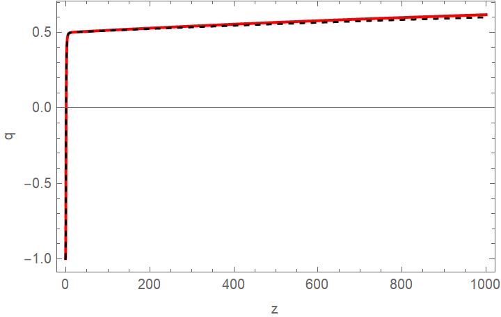
Figure 4: The deceleration parameter $q$ for the $f(R)$ gravity model (red curve) and the $\Lambda$CDM model (black dashed curve).

Also in Table 1 we present the values of the dark energy EoS parameter and of the dark energy density parameter at present day and we compare these with the latest Planck constraints [84]. Also we quote the value of the deceleration parameter at present day for the $f(R)$ gravity model and the $\Lambda$CDM model.

Table 1: Values of Cosmological Parameters for $f(R)$ Gravity Model and $\Lambda$CDM Model.

Cosmological Parameter	$f(R)$ Gravity Value	Base $\Lambda$CDM or Planck 2018 Value
$\Omega_{DE}(0)$	0.683951	$0.6847\pm 0.0073$
$\omega_{DE}(0)$	-0.995258	$-1.018\pm 0.031$
$q(0)$	-0.521012	-0.535

The whole analysis indicates that the dark energy era and the epochs before it for the $f(R)$ gravity model are quite successful and mimic to a great extend the $\Lambda$CDM model, with the difference being that the statefinder $y_{H}$ is dynamical for the $f(R)$ gravity model and the dark energy EoS parameter is not constant, but dynamically evolving.

Let us now proceed to the core of our analysis for the $f(R)$ gravity model at hand, and the calculation of the parameter $a_{M}$ (51), the “damping” factor $\mathcal{D}$ (50) and subsequently the gravitational wave energy spectrum (29). In Fig. 5 we plot the parameter $a_{M}$ (51) as a function of the redshift. It is apparent that beyond $z=1000$ the parameter $a_{M}$ oscillates and thus the integral (50) receives insignificant contribution beyond $z=1000$, a fact that we verified numerically by solving the equations numerically for up to $z=10000$.

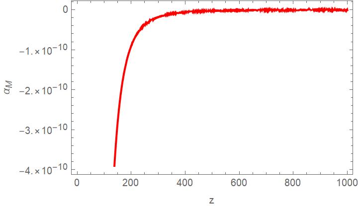
Figure 5: The parameter $a_{M}$ (51) for the $f(R)$ gravity model for $z=[0,1000]$.

Thus performing the integral (50) numerically, we obtain $\mathcal{D}=-0.00451304/2$ therefore the total “damping” factor is for the model at hand $e^{-2\mathcal{D}}=e^{0.00451304}=1.00452$ for redshifts up to $z_{fin}=1000$. Also for redshifts corresponding to the radiation domination era, the parameter $a_{M}$ is equal to zero since $\dot{R}=0$ for $\omega_{tot}=1/3$ and also the term $f_{RR}/f_{R}$ for $R\to 0$ and for the model at hand is zero. Thus the only contribution to the integral (50) is from the interval $z=[0,1000]$, hence for this particular model, the GR waveform is almost identical with the $f(R)$ gravity waveform. Therefore, the gravitational wave spectrum for the $f(R)$ gravity model at hand is,

$$\Omega_{\rm gw}(f)=1.00452\times\frac{k^{2}}{12H_{0}^{2}}r\mathcal{P}_{\zeta}(k_{ref})\left(\frac{k}{k_{ref}}\right)^{n_{T}}\times$$ (99)

$$\left(\frac{\Omega_{m}}{\Omega_{\Lambda}}\right)^{2}\left(\frac{g_{*}(T_{\rm in})}{g_{*0}}\right)\left(\frac{g_{*s0}}{g_{*s}(T_{\rm in})}\right)^{4/3}\left(\overline{\frac{3j_{1}(k\tau_{0})}{k\tau_{0}}}\right)^{2}T_{1}^{2}\left(x_{\rm eq}\right)T_{2}^{2}\left(x_{R}\right)$$

where the parameters appearing in Eq. (99) are defined below Eq. (29). Now since $\tau_{0}=14379.2$ Mpc, and by taking a reheating temperature of the order $T_{R}\sim 10^{7}$GeV, in Fig. 6 we plot the $h^{2}$-scaled gravitational wave spectrum taking also into account that $\mathcal{P}_{\zeta}(k_{ref})\simeq 20.0855\times 10^{-10}$ for the latest Planck constraints on inflation [83].

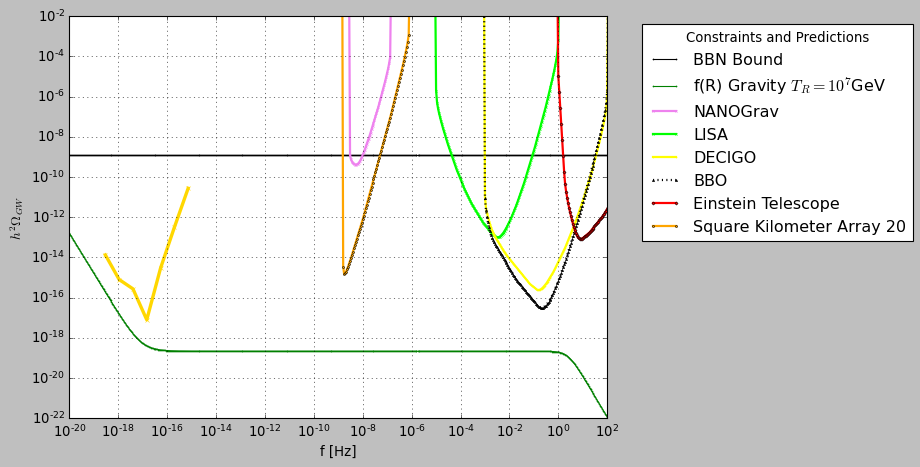
Figure 6: The $h^{2}$-scaled gravitational wave energy spectrum for pure $f(R)$ gravity.

Apparently, the results obtained from Fig. 6 are strict and rigid. The signal of the gravitational wave spectrum for the model of $f(R)$ gravity we discussed in this section, cannot be detected by any of the future experiments and missions. Thus this offers a perspective for future studies: If a signal is not detected by LISA or Litebird or BBO and DECIGO, this would not necessarily mean that inflation never took place, but possibly that the sensitivities of the experiments are not adequate to capture this signal. We tried a large number of pure $f(R)$ gravity models which we chose not to present and the result seems to be robust for all the models, the signal is lower compared to the sensitivities of the experiments. The reheating temperature seems not to affect the result and the same applies for the initial conditions we chosen to numerically integrate the Friedmann equation for large redshifts. The only thing that seems to crucially affect the resulting signal is the tensor spectral index, and specifically if it is positive, then the signal of the primordial gravitational waves spectrum might be detectable by the future experiments. However a positive spectral index cannot be obtained for $f(R)$ gravity as it is apparent from Eq. (80). Hence in order to obtain a positive spectral index for $f(R)$ gravity, one needs to include other modified gravity terms in the inflationary Lagrangian. A model of this sort is presented in the next section.

III.2 Unified Description of Inflation and Dark Energy II: A Chern-Simons Corrected $k$-essence $f(R)$ Gravity Model

In this section we shall consider another interesting toy model which has two unique characteristics, firstly it describes in a unified way and successfully both the inflationary era and the late-time era, and secondly and more importantly it generates detectable gravitational wave energy spectrum. Also the generated spectrum has two distinct signals, which is due to the presence of a Chern-Simons term. The toy model is a Chern-Simons $k$-essence $f(R)$ gravity theory, and the motivation for using such an extension was mainly the production of a blue tilted tensor spectral index. As we saw in the previous section $f(R)$ gravity produces a red-tilted tensor spectral index, thus an extension of pure $f(R)$ gravity is needed in order to produce a blue-tilted tensor spectral index. Apart from the possibility of producing a blue-tilted tensor spectral index, the model eventually produces two distinct signals in the energy spectrum of the primordial gravitational waves, which is a quite intriguing feature and a prediction for future predictions.

Let us commence with the specification of the gravitational action. As we already mentioned, we shall examine the phenomenological implications of a potential-less $k$-essence $f(R)$ gravity in the presence of a Chern-Simons term corresponding to the following action,

$$\centering S=\int{d^{4}x\sqrt{-g}\left(\frac{f(R)}{2\kappa^{2}}+G(X)+\frac{1}{8}\nu(\phi)\eta^{abcd}R_{ab}^{\ \ ef}R_{cdef}\right)}\,,\@add@centering$$ (100)

with $f(R)$ being an arbitrary for the time being function depending solely on the Ricci scalar, $\kappa=\frac{1}{M_{P}}$ stands for the gravitational constant with $M_{P}$ being the reduced Planck mass, $G(X)$ is also an arbitrary function that depends on the kinetic term of the scalar field $X=\frac{1}{2}\nabla_{\mu}\phi\nabla^{\mu}\phi$, $\nu(\phi)$ signifies the Chern-Simons scalar coupling function coupled to the antisymmetric term. For the purpose of this paper we shall limit our work to the case of a homogeneous and isotropic expansion corresponding to a FRW metric. As a consequence, it is reasonable to assume that the scalar field itself is also homogeneous, therefore the kinetic term is simplified significantly. For the sake of consistency we mention that hereafter the previously introduced functions and auxiliary parameters have the following form,

$$\centering f(R)=R+\alpha R^{2}-(R+R_{0})P_{3}\left(\frac{M_{P}^{2}}{R+R_{0}}\right)\,,\@add@centering$$ (101)

with $\alpha=\frac{1}{36H_{i}}$ and,

$$\centering G(X)=-X-f_{1}\kappa^{4}X^{2},\,\,\,X=-\frac{1}{2}\dot{\phi}^{2},\,\,\,\phi(t)=\frac{t}{\kappa^{2}f_{1}^{\frac{1}{3}}}\,,\@add@centering$$ (102)

where the parameter $H_{i}$ has mass dimensions $[H_{i}]=$eV², and $P_{3}(x)$ in Eq. (101) is the Legendre polynomial of degree three. Note that in Eq. (102) the expression of the scalar field is taken from Ref. [89] for the case of $k$-Essence models during the inflationary era. The corresponding continuity equation for the scalar field reads,

$$\centering 3f_{1}2^{1-m}mH\dot{\phi}^{2m-1}-3H\dot{\phi}-\ddot{\phi}f_{1}2^{2-m}m^{2}\dot{\phi}^{2}-\ddot{\phi}-\dot{\phi}^{2m-4}-f_{1}^{2}2^{-m}m\dot{\phi}^{2m-2}\ddot{\phi}+2^{-m}m\ddot{\phi}\dot{\phi}^{2m-2}=0\,,\@add@centering$$ (103)

therefore by keeping the leading order terms in the aforementioned equation, one finds,

$$\centering 3f_{1}2^{1-m}mH\dot{\phi}^{2m}-3H\dot{\phi}=0\,,\@add@centering$$ (104)

from which the solution for $\phi(t)$ appearing in Eq. (102) emerges for the case of $m=2$.

As it can easily be seen, the Legendre polynomial related term of the $f(R)$ gravity in the large curvature limit, which basically describes inflation, behaves as follows,

$$\lim_{R\to\infty}(R+R_{0})P_{3}\left(\frac{M_{P}^{2}}{R+R_{0}}\right)\simeq\frac{15M_{P}^{6}R_{0}^{2}}{2R^{4}}-\frac{5\left(M_{P}^{6}R_{0}\right)}{R^{3}}+\frac{5M_{P}^{6}}{2R^{2}}-\frac{3M_{P}^{2}}{2}+\mathcal{O}(1/R^{5})\,,$$ (105)

thus during the inflationary era the Legendre polynomial related term merely contributes a cosmological constant. Also at late times, the same term in the small curvature regime at leading order contributes a cosmological constant, since,

$$\lim_{R\to 0}(R+R_{0})P_{3}\left(\frac{M_{P}^{2}}{R+R_{0}}\right)\simeq\frac{15M_{P}^{6}R^{2}}{2R_{0}^{4}}-\frac{10M_{P}^{6}R^{3}}{R_{0}^{5}}-\frac{5M_{P}^{6}R}{R_{0}^{3}}+\frac{5M_{P}^{6}-3M_{P}^{2}R_{0}^{2}}{2R_{0}^{2}}\,.$$ (106)

Thus during inflation, the term that drives the inflationary era is the $R^{2}$ term and at late times the cosmological constant appearing in Eq. (106) basically determines the evolution. As we will show numerically, the dark energy era corresponds to a pure cosmological constant non-dynamical behavior, in contrast to the $f(R)$ gravity case considered in the previous section.

In order to properly study the inflationary era we shall focus mainly on the slow-roll indices [81], designated as,

$$\centering\epsilon_{1}\@add@centering =-\frac{\dot{H}}{H^{2}} \epsilon_{2} =\frac{\ddot{\phi}}{H\dot{\phi}} \epsilon_{3} =\frac{\dot{f}_{R}}{2Hf_{R}} \epsilon_{4} =\frac{\dot{E}}{2HE} \epsilon_{6} =\sum_{l}\frac{\dot{Q}_{t}}{2HQ_{t}}\,,$$ (107)

where $f_{R}=\frac{df}{dR}$, $E=-\frac{f_{R}}{X}\left(XG_{,X}+2X^{2}G_{,XX}+\frac{3\dot{f}_{R}^{2}}{2\kappa^{2}f_{R}}\right)$ and $Q_{t}=f_{R}+2\lambda_{l}\kappa^{2}\dot{\nu}H$, where $l$ sums over the polarizations of the gravitational waves with $\lambda_{l}=\pm 1$ for left and right handed polarization respectively. It is worth mentioning that the second slow-roll index is identically equal to zero since the scalar field evolves primordially linearly with respect to time. Knowledge of the slow-roll indices is essentially important as the observational indices can be extracted from them. Let us now study each slow-roll index separately and derive certain conclusions.

Obviously, as mentioned before, $\ddot{\phi}=0$ therefore $\epsilon_{2}=0$. Now according to Eq.(107), we have,

$$\centering\epsilon_{1}=-\frac{\dot{H}}{H^{2}}\,,\@add@centering$$ (108)

and since the $R^{2}$ term drives the early-time era and specifically the Friedmann equation, the Hubble rate during inflation is perfectly described by the quasi-de Sitter expansion $H(t)=H_{0}-H_{i}t$ (see Ref. [75] for details). We shall further support this result of a quasi-de Sitter evolution later on, when we consider specific forms of the Chern-Simons coupling function (see the arguments below Eq. (129)). Thus, the first slow-roll index reads,

$$\centering\epsilon_{1}=\frac{H_{i}}{H_{0}^{2}\left(1-\frac{H_{i}t_{i}}{H_{0}}\right)^{2}}\,,\@add@centering$$ (109)

In order to ascertain the time duration of the inflationary era we assume that the first slow-roll index reaches unity. Solving $\epsilon_{1}(t_{f})\sim\mathcal{O}(1)$ we find that,

$$\centering t_{f}=\left(1\mp\frac{\sqrt{H_{i}}}{H_{0}}\right)\frac{H_{0}}{H_{i}}\,,\@add@centering$$ (110)

This signifies the time instance in units of eV^-1 when the inflationary era ceases and of course the positive solution is relevant. In consequence, from the definition of the $e$-foldings number $N=\int_{t_{i}}^{t_{f}}{H(t)dt}$, the initial time $t_{i}$ for which inflation starts, can be computed and reads,

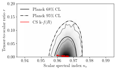
Figure 7: Planck 2018 likelihood curves and the Chern-Simons $k$-essence $f(R)$ gravity inflationary predictions for $N=[50,60]$ and $f_{1}=2\times 10^{N}$.

$$\centering t_{i}=c_{1}+\sqrt{c_{1}^{2}+c_{2}}\,,\@add@centering$$ (111)

where we keep only the positive solution as $c_{2}>0$ and the auxiliary parameters read $c_{1}=\frac{H_{0}}{H_{i}}$ and $c_{2}=t_{f}^{2}+\frac{2N}{H_{i}}-\frac{2H_{0}t_{f}}{H_{i}}$. The initial time is of paramount importance as the observational indices are extracted by evaluating the slow-roll indices an mentioned before, at exactly that time instance, which signifies the first horizon crossing during inflation. Let us now proceed with the rest slow-roll indices. For the slow-roll index $\epsilon_{3}$, we have,

$$\centering R\@add@centering \simeq 12H^{2} f_{R} \simeq 1+2\alpha R \dot{f}_{R} \simeq 2\alpha\dot{R}\,,$$ (112)

so if we assume contribution from the $R^{2}$ part since it is more dominant during the inflationary era, we find that $\epsilon_{3}\simeq-\epsilon_{1}$ and their difference due to unity in $f_{R}$ is of order $\mathcal{O}\left(\frac{1}{N^{2}}\right)$ something which has an impact on the tensor-to-scalar ratio. Now for slow-roll index $\epsilon_{4}$, we have $\epsilon_{4}=\frac{\dot{E}}{2HE}$ with,

$$\centering E=-\frac{f_{R}}{X}\left(XG_{,X}+2X^{2}G_{,XX}+\frac{3\dot{f}_{R}^{2}}{2\kappa^{2}f_{R}}\right)=f_{R}\left(1+6f_{1}\kappa^{4}X-\frac{3\dot{f}_{R}^{2}}{2\kappa^{2}f_{R}X}\right)\,,\@add@centering$$ (113)

The final part scales with $\frac{1}{N^{2}}$ so it is significantly subdominant, therefore we find that $\epsilon_{4}\simeq-\epsilon_{1}$. Overall the scalar spectral index reads,

$$\centering n_{S}=1-2(2\epsilon_{1}+\epsilon_{2}-\epsilon_{3}+\epsilon_{4})\simeq 1-\frac{2}{N}+\mathcal{O}\left(\frac{1}{N^{2}}\right)\,,\@add@centering$$ (114)

Note that $\frac{1}{N^{2}}$ corrections come from the difference between $\epsilon_{3}$ and $\epsilon_{1}$ while $\mathcal{O}(\frac{1}{N^{3}})$ comes from the neglected term in $\epsilon_{4}$ so the overall phenomenology seems quite right. As shown, it coincides with the exact form of the $R^{2}$ model. Now for the tensor-to-scalar ratio, according to Ref. [81], we have,

$$\centering r=8|\epsilon_{1}+\epsilon_{3}|c_{A}\sum_{l}\frac{1}{\left|1+\frac{2\lambda_{l}\kappa^{2}\dot{\nu}H}{f_{R}}\right|}\,.\@add@centering$$ (115)

From the definition of the sound wave velocity, we find that,

$$\centering c_{A}=\sqrt{\frac{XG_{,X}+\frac{3\dot{f}_{R}^{2}}{2\kappa^{2}f_{R}}}{XG_{,X}+2X^{2}G_{,XX}+\frac{3\dot{f}_{R}^{2}}{2\kappa^{2}f_{R}}}}=\sqrt{\frac{1-f_{1}^{\frac{1}{3}}}{1-3f_{1}^{\frac{1}{3}}}}+\mathcal{O}\left(\frac{1}{N^{2}}\right)\,,\@add@centering$$ (116)

if we perform a Taylor expansion for large $N$ in the $\frac{\dot{f}_{R}^{2}}{2\kappa^{2}f_{R}X}$ term. Moreover, the Chern-Simons contribution during the first horizon crossing, if one replaces $H(t_{i})$ in $f_{R}$ then the following expression emerges,

$$\centering r\simeq\frac{6}{N^{2}}\sqrt{\frac{1-f_{1}^{\frac{1}{3}}}{1-3f_{1}^{\frac{1}{3}}}}\left(\frac{1}{\left|1+\frac{3\kappa^{2}\dot{\nu}\sqrt{H_{i}}}{\sqrt{2N}}\right|}+\frac{1}{\left|1-\frac{3\kappa^{2}\dot{\nu}\sqrt{H_{i}}}{\sqrt{2N}}\right|}\right)\,,\@add@centering$$ (117)

Here, two main features are mentionable. Firstly, the case of the $R^{2}$ model’s tensor-to-scalar ratio, meaning $r\simeq\frac{12}{N^{2}}$ can be extracted from the above expression by choosing $\nu=0$ and $f_{1}=0$, therefore the known results of the $R^{2}$ gravity are safely extracted. Furthermore, due to the presence of a non-canonical kinetic term, the field propagation velocity satisfies the relation $c_{A}<1$ thus the $k$-essence term results in a decrease of the tensor-to-scalar ratio relative to the expected $\frac{12}{N^{2}}$. For the time being, no conclusion can be extracted for the time derivative of the Chern-Simons scalar coupling function and therefore the additional contribution in Eq. (117). The result should be considered to be model-dependent.

Finally, for the tensor spectral index, we need $\epsilon_{1}\simeq\frac{1}{2N}$ and $\epsilon_{6}=\sum_{l}\frac{\dot{Q}_{t}}{2HQ_{t}}$ where $Q_{t}(t_{i})=f_{R}(t_{i})+2\lambda_{l}\kappa^{2}\dot{\nu}H(t_{i})$. If we evaluate the ratio $\frac{\dot{Q}_{t}}{2HQ_{t}}$ we find,

$$\centering\frac{\dot{Q}_{t}}{2HQ_{t}}\Big{|}_{t_{i}}=\epsilon_{3}\left(\frac{1+\frac{\lambda_{l}\kappa^{2}\dot{\nu}H}{f_{R}}}{1+\frac{2\lambda_{l}\kappa^{2}\dot{\nu}H}{f_{R}}}\right)+\frac{\lambda_{l}\kappa^{2}\ddot{\nu}}{f_{R}\left(1+\frac{2\lambda_{l}\kappa^{2}\dot{\nu}H}{f_{R}}\right)}\,,\@add@centering$$ (118)

where hereafter everything is evaluated at the first horizon crossing. It is tempting, to say the least, to argue that under the slow-roll assumption the first part is almost equal to $\epsilon_{3}$, however this is not the case here since the functions $\ddot{\nu}$ and $\dot{\nu}$ could be more dominant, therefore one needs to keep such term as it is and evaluate it numerically. In general, we have,

$$\centering\epsilon_{6}=\epsilon_{3}\sum_{l}\left(\frac{1+\frac{\lambda_{l}\kappa^{2}\dot{\nu}H}{f_{R}}}{1+\frac{2\lambda_{l}\kappa^{2}\dot{\nu}H}{f_{R}}}\right)-\frac{\frac{4\kappa^{4}\ddot{\nu}\dot{\nu}H}{f_{R}^{2}}}{1-\frac{4\kappa^{4}\dot{\nu}^{2}H^{2}}{f_{R}^{2}}}\,,\@add@centering$$ (119)

and by focusing on the case of $1\ll\frac{\lambda_{l}\kappa^{2}\dot{\nu}H}{f_{R}}$, one finds that,

$$\centering\epsilon_{6}=\epsilon_{3}-\frac{\frac{4\kappa^{4}\ddot{\nu}\dot{\nu}H}{f_{R}^{2}}}{1-\frac{4\kappa^{4}\dot{\nu}^{2}H^{2}}{f_{R}^{2}}}\,,\@add@centering$$ (120)

One would make the approximation $\epsilon_{3}\simeq-\epsilon_{1}$ however this could result in a zero tensor spectral index for the case of $\ddot{\nu}\ll\dot{\nu}^{2}$, and this is true at first order. However, if we recall that for inflationary $f(R)$ attractors, as we saw previously, the slow-roll indices are interconnected as $\epsilon_{1}=-\epsilon_{3}(1-\epsilon_{4})$ therefore in our case, $\epsilon_{3}=-\epsilon_{1}+\epsilon_{3}\epsilon_{4}$ and $\epsilon_{4}\simeq-\epsilon_{1}$, therefore to leading order, $\epsilon_{3}=-\epsilon_{1}+\epsilon_{1}^{2}$ thus the tensor spectral index reads,

$$\centering n_{T}=-2\epsilon_{1}^{2}+\frac{\frac{8\kappa^{4}\ddot{\nu}\dot{\nu}H}{f_{R}^{2}}}{1-\frac{4\kappa^{4}\dot{\nu}^{2}H^{2}}{f_{R}^{2}}}\,,\@add@centering$$ (121)

where it becomes apparent that for the case of $\nu=0$, the result coincides with the one obtained for the $R^{2}$ model developed in the previous section. Before we proceed, it is worth mentioning that due to the fact that $\epsilon_{6}$ is proportional to $-\epsilon_{1}$, the tensor spectral index receives positive contribution to order $\mathcal{O}\left(\frac{1}{N^{2}}\right)$.

If we focus on the numerator and denominator separately and evaluate everything during the first horizon crossing, then a term $\frac{9\kappa^{4}\ddot{\nu}\dot{\nu}\sqrt{H_{i}}}{\sqrt{2}N^{\frac{3}{2}}}\frac{1}{1-\frac{9\kappa^{4}\dot{\nu}^{2}H_{i}}{f_{R}^{2}}}$ appears, if we expand in powers of $N$ in the large $N$ limit, then a term of order $\mathcal{O}\left(\frac{1}{N^{\frac{5}{2}}}\right)$ emerges in the tensor spectral index, and we treat it as subleading. Overall we find,

$$\centering n_{T}\simeq-\frac{1}{2N^{2}}+\frac{9\kappa^{4}\ddot{\nu}\dot{\nu}\sqrt{H_{i}}}{\sqrt{2}N^{\frac{3}{2}}}+\mathcal{O}\left(\frac{1}{N^{\frac{5}{2}}}\right)\,,\@add@centering$$ (122)

Depending on the sign/dominance of the first term, the tensor spectral index may be blue-tilted. Note also that in principle $\ddot{\nu}=\dot{\phi}^{2}\nu^{\prime\prime}$ given that $\ddot{\phi}=0$. Now, if we use the fact that $H_{i}=\frac{M^{2}}{6}$, such that $f(R)=R+\frac{R^{2}}{6M^{2}}$ we find that with respect to such mass scale the observational indices become,

$$\centering n_{S}\@add@centering \simeq 1-\frac{2}{N}+\mathcal{O}\left(\frac{1}{N^{2}}\right)$$ (123)

$$r \simeq\frac{6}{N^{2}}\sqrt{\frac{1-f_{1}^{\frac{1}{3}}}{1-3f_{1}^{\frac{1}{3}}}}\left(\frac{1}{\left|1+\frac{3\kappa^{2}\dot{\nu}M}{2\sqrt{3N}}\right|}+\frac{1}{\left|1-\frac{3\kappa^{2}\dot{\nu}M}{2\sqrt{3N}}\right|}\right)+\mathcal{O}\left(\frac{1}{N^{4}}\right)$$ (124)

$$n_{T} \simeq-\frac{1}{2N^{2}}+\frac{9\kappa^{4}\ddot{\nu}\dot{\nu}M}{2\sqrt{3}N^{\frac{3}{2}}}+\mathcal{O}\left(\frac{1}{N^{\frac{5}{2}}}\right)\,,$$ (125)

Truthfully, the final form of the tensor spectral index is possible only if $\kappa^{3}\ddot{\nu}\dot{\nu}$ is well behaved, however in this case the ratio in front of $\epsilon_{3}$ in (119) would be closer to unity for a given polarization $l$, thus instead of $\frac{1}{2N^{2}}$ a factor of $\frac{1}{N}$ would emerge. Therefore only in such case the expansion is permitted, however for the $k$-essence model where the $\dot{\nu}$ function is quite large, as we shall showcase below, Eq. (121) should be used in the following form

$$\centering n_{T}\simeq-\frac{1}{2N^{2}}+\frac{\frac{9\kappa^{4}\ddot{\nu}\dot{\nu}M}{2\sqrt{3N}N}}{1-\frac{3\dot{\nu}^{2}\kappa^{2}M^{2}}{4N}}\,,\@add@centering$$ (126)

The resulting behavior is model-dependent as we shall showcase briefly. To prove this, we shall use certain power-law and exponential models for the Chern-Simons scalar coupling function, and the exponential shall be used for the primordial and late-time evolution study, and for the calculation of the primordial gravitational wave energy power spectrum.

Let us start with the case of,

$$\centering\nu(\phi)=\Lambda_{1}(\kappa\phi)^{2}\,,\@add@centering$$ (127)

then for the case of $\Lambda_{1}=100$, $f_{1}=-20$ and $N=60$ we find that $r=0.000209$ and $n_{T}=-0.083879$ while for an increasing $\Lambda_{1}$ the tensor to scalar ratio decreases due to the Chern-Simons term. The result is extracted by making use of Eq. (126) otherwise one would find a diverging tensor spectral index given that $\dot{\phi}\sim 10^{55}$eV² during the first horizon crossing. So we see that the expansion in large $N$ in the presence of a $k$-Essence term is not a viable option for the case of the tensor spectral index, due to the Chern-Simons term. In fact, the Chern-Simons contribution becomes so dominant that the sign of the tensor spectral index switches and becomes negative.

Let us examine now a different model. Suppose that,

$$\centering\nu(\phi)=\Lambda_{1}\phi\,,\@add@centering$$ (128)

with $\Lambda_{1}\sim\mathcal{O}(10^{400})$, $f_{1}\sim\mathcal{O}(1)$ and $N\sim 60$, then due to the fact that $\ddot{\phi}$ is identically zero the tensor spectral index is positive and equal to $n_{T}=0.00014$ whereas due to the extreme value of $\Lambda_{1}$ the tensor-to-scalar ratio is suppressed to $r=0$. The aforementioned model is indicative of the fact that the scalar field assisted $f(R)$ gravity can be used in order to properly describe both early and late-time eras in a unified manner and also make significant predictions for gravitational waves and future experiments.

Finally we introduce the model we shall work with in the following sections. This particular model admits an exponential Chern-Simons scalar coupling function of the form,

$$\centering\nu(\phi)=\Lambda_{1}e^{\sqrt{\frac{\phi}{M_{1}}}}\,,\@add@centering$$ (129)

where $\Lambda_{1}=4\cdot 10^{-12}$ and $M_{1}=25\cdot 10^{-5.332}\Lambda_{1}M_{P}$. For this particular model and with the assumption that $f_{1}=2\cdot 10^{N}$ and $N=54.2$ one finds using equations (117) and (126) that the tensor to scalar ratio and the tensor spectral index respectively obtain the values $r=0.003165$ and $n_{T}=0.01659$. We shall use these values for the calculation of the gravitational wave energy spectrum later on. In Fig. 7 we present the Planck 2018 likelihood curves and the inflationary predictions of the Chern-Simons $k$-essence $f(R)$ gravity model for $N=[50,60]$ and $f_{1}=2\times 10^{N}$ (red curve). As it can be seen in Fig. 7 the Chern-Simons $k$-essence $f(R)$ gravity model is well fitted in the Planck data. It is worth mentioning that the number of free parameters is effectively decreased to 3, namely $\Lambda_{1}$, $M$ and $N$ given that $M_{1}$ and $f_{1}$ are now functions of $\Lambda_{1}$ and $N$ respectively whereas the $R^{2}$ scale is assumed to be equal to $M=1.25\cdot 10^{-5}M_{P}$ similar to the previous power-law cases. Note that such designation suggests that the tensor spectral index is blue tilted which in turn suggests that the denominator in equation (126) is more dominant than the numerator. The case of large $f_{1}$ and $\dot{\nu}$ results in a finite ratio between the field propagation velocity and the Chern-Simons contribution in the tensor-to-scalar ratio (117), therefore it is non zero, but as expected it satisfies the relation $r<\frac{12}{N^{2}}$. Note also that decreasing $f_{1}$ and essentially not-constraining it, the $e$-foldings number can result in principle in a negative tensor spectral index. As a final note it should be stated that for the case of $N>54$, working with the expression for $n_{T}$ extracted in Eq. (123) is a viable choice as it produces the same result with (126), something which can be seen from Fig. 8, where we plot the tensor-to-scalar ratio $r$ (left) and tensor spectral index $n_{T}$ (right) as functions of the $e$-foldings number and with the parameter $f_{1}$ being chosen $f_{1}=2\cdot 10^{N}$. As shown, the value of $N=54$ serves as a boundary for which the sign of the tensor spectral index changes and above which the approximated solution for $n_{T}$ extracted before can safely be used. This is a model dependent result and applies only for the exponential Chern-Simons scalar coupling function. For the order of magnitude, $\dot{\phi}\sim 10^{37}eV^{2}$ and $R^{2}\sim 10^{90}eV^{2}$ assuming that $H\sim 10^{13}GeV$ therefore, the $R^{2}$ contribution is more dominant in the inflationary era compared to the $k$-essence part, thus validating the choice of the quasi-de Sitter expansion.

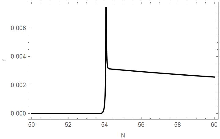
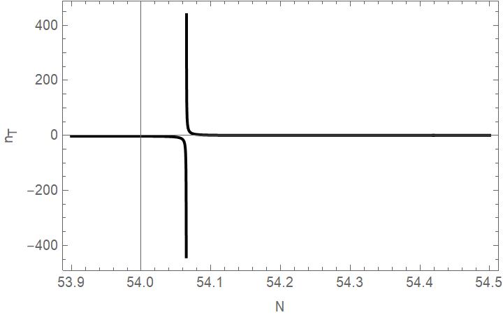
Figure 8: Tensor to scalar ratio $r$ (left) and tensor spectral index $n_{T}$ (right) depending on the e-folding number and parameter $f_{1}$ satisfying the condition $f_{1}=2\cdot 10^{N}$.

The exponential model we just discussed, shall be used subsequently to study the late-time phenomenology of the Chern-Simons $k$-essence $f(R)$ model, and for the evaluation of the primordial gravitational wave energy spectrum. Due to the fact that the signal of pure $f(R)$ gravity models is quite suppressed relative to the current detectable amplitudes from present and future missions and experiments, such as the NANOGrav, LISA, DECIGO etc., it can be shown that the inclusion of a cosmological scalar field can actually contribute both in the late-time description and can significantly affect the energy spectrum of the gravitational waves of inflation.

III.3 From the Dark Energy Era to Radiation Domination Era for the Chern-Simons $k$-essence $f(R)$ Gravity and the Primordial Gravitational Waves Spectrum

Figure 9: Numerical solutions for statefinder $y_{H}$ and the scalar field normalized with the Planck mass as functions of redshift. It becomes apparent that while $y_{H}$ is constant in time, meaning that it behaves effectively as a cosmological constant corresponding to constant dark energy density and in consequence constant dark energy EoS, the scalar field seems to decrease with time.

Having discussed the inflationary phenomenology of the model (101), let us now consider the evolution of the model during the various cosmological eras, from the dark energy era back to the radiation domination era. We shall transform all the field equations in such a way so that the variable will be the statefinder $y_{H}(z)$ we used in the pure $f(R)$ gravity section, and the dynamical variable will be the redshift $z$. Our aim is to calculate the overall “damping” factor $\mathcal{D}$ thus to calculate the integral of the parameter (60). The upper limit of the redshift integration will be determined approximately to be the redshift for which the cosmological model enters the radiation domination era, and as it proves it is approximately $z_{fin}=400000$. Beyond that, parameter $a_{M\ell}$ gets simplified to the form (152) and as it proves, the integral (50) receives no contribution beyond the upper redshift $z_{fin}=400000$.

The main focus in this section lies in the numerical solution of the equations of motion and in particular both the Friedmann equation and the continuity equation of the scalar field which was introduced previously during the inflationary era. For the sake of generality, an arbitrary minimally coupled scalar-tensor model, an in particular a $k$-essence $f(R)$ model shall be presented but subsequently we shall focus mainly on the $R^{2}$ model with an exponential Chern-Simons coupling.

Let us commence from the equations of motion. For an arbitrary minimal scalar-tensor model in the presence of perfect fluids, the Friedman and continuity equation for the scalar field read

$$\centering\frac{3f_{R}H^{2}}{\kappa^{2}}=\rho+\frac{f_{R}R-f}{2\kappa^{2}}-\frac{3H\dot{f}_{R}}{\kappa^{2}}+G_{,X}X-\frac{G}{2}\,,\@add@centering$$ (130)

$$\centering G_{,X}(\ddot{\phi}+3H\dot{\phi})+\dot{\phi}\dot{G}_{,X}=0\,,\@add@centering$$ (131)

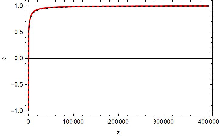
Figure 10: The deceleration parameter versus the redshift for the Chern-Simons $k$-essence $f(R)$ gravity model versus the redshift (red curve). The black dashed curve corresponds to the $\Lambda$CDM model

The main focus lies with the numerical solution of Hubble’s parameter and the scalar field, as functions of cosmic time $t$. This procedure is intricate and thus certain transformations are needed in order to facilitate the study of the late-time era and essentially work backwards and study the matter and radiation dominated eras respectively. In order to proceed, two transformations need to be performed that facilitate the overall procedure. The first transformation is a variable transformation and is used in order to replace cosmic time $t$ with redshift though the definition of redshift,

$$\centering 1+z=\frac{1}{a}\,,\@add@centering$$ (132)

where for simplicity it was assumed that the current value of the scale factor is normalized to unity in order for the comoving wavelengths and physical wavelengths to coincide at present time. Essentially one can think of such definition as a function of the form $t=t(z)$, therefore a connection between time derivatives and derivatives with respect to redshift is needed. This connection emerges naturally from Eq. (132) by means of construction of a differential operator that connects these two variables. This operator reads,

$$\centering\frac{d}{dt}=-H(1+z)\frac{d}{dz}\,,\@add@centering$$ (133)

with the Hubble rate now being a function of redshift itself. For simplicity, differentiation with respect to redshift shall be denoted with prime $\frac{d}{dz}=^{\prime}$. Therefore, certain time derivatives which participate in the aforementioned equations of motion are transformed as,

$$\centering\dot{H}\@add@centering =-H(1+z)H^{\prime}$$ (134)

$$\dot{\phi} =-H(1+z)\phi^{\prime}$$ (135)

$$\dot{R} =-H(1+z)R^{\prime}$$ (136)

where the last participates in the Friedmann equation through $\dot{f}_{R}=f_{RR}\dot{R}$. Performing such replacements in equations (130)-(131) eliminates cosmic time $t$, as expected, however working with Hubble itself is a bit intricate as it has mass dimensions $[m]=$eV.

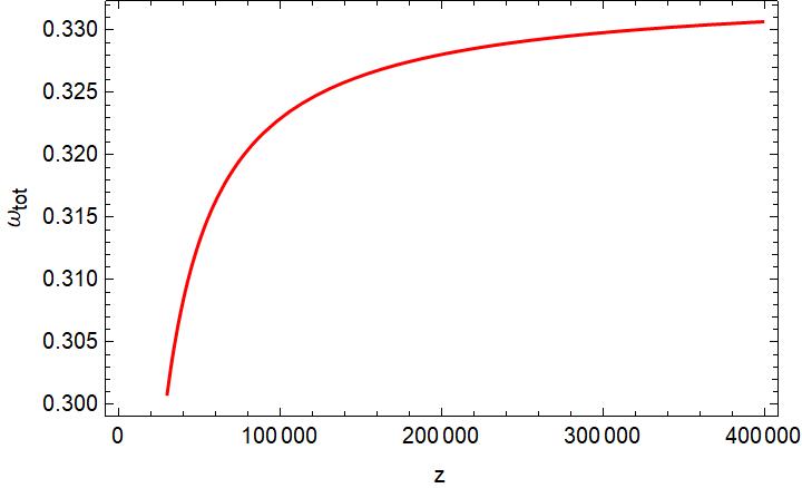
Figure 11: The total EoS parameter for the Chern-Simons S-$k$-essence $f(R)$ gravity model.

Instead, one can work with a new dimensionless variable which can be derived from the Friedmann equation. In particular, by rewriting Eq. (130) in the usual form the Friedmann equation has, the following expression is derived,

$$\centering\frac{3H^{2}}{\kappa^{2}}=\rho+\rho_{DE}\,,\@add@centering$$ (137)

where the new contribution specifies dark energy at late times and is specified as,

$$\centering\rho_{DE}=\frac{f_{R}R-f}{2\kappa^{2}}-\frac{3H\dot{f}_{R}}{\kappa^{2}}+G_{,X}X-\frac{G}{2}+\frac{3H^{2}}{\kappa^{2}}(1-f_{R})\,,\@add@centering$$ (138)

Here, it becomes abundantly clear that the dark energy density, and in general the definition of the dark energy, is nothing but the contribution of all geometric terms which appear in the gravitational action and in consequence the Friedmann equation. Subsequently, we define the dimensionless statefinder parameter $y_{H}$, as in the pure $f(R)$ gravity section,

$$\centering y_{H}(z)=\frac{\rho_{DE}}{\rho_{0}}=\frac{H^{2}}{m_{s}^{2}}-\frac{\rho}{\rho_{m}^{(0)}}\,,\@add@centering$$ (139)

where $\rho_{m}^{(0)}$ is the current density of non relativistic matter and $m_{s}^{2}=\frac{\kappa^{2}\rho_{m}^{(0)}}{3}$ serves as a mass scale which were defined in the pure $f(R)$ gravity section. This statefinder in particular is used for replacing Hubble’s parameter in the equations of motion which shall be solved numerically. Furthermore the matter density is given by the formula,

$$\centering\rho=\rho_{m}^{(0)}(1+z)^{3}(1+\chi(1+z))\,,\@add@centering$$ (140)

where $\chi=\frac{\rho_{r0}}{\rho_{m}^{(0)}}$ serves as a ratio between the current value of relativistic and non relativistic matter density. Therefore, by replacing Hubble’s parameter with the statefinder $y_{H}$, the numerical solution of equations (130)-(131) becomes easier to extract. In particular, we mention that the replacement of Hubble’s parameter is achieved though the subsequent replacements,

$$\centering H\@add@centering =m_{s}\sqrt{y_{H}+\tilde{\rho}}$$ (141)

$$HH^{\prime} =\frac{m_{s}^{2}}{2}(y_{H}^{\prime}+\tilde{\rho}^{\prime})$$ (142)

$$H^{\prime 2}+HH^{\prime\prime} =\frac{m_{s}^{2}}{2}(y_{H}^{\prime\prime}+\tilde{\rho}^{\prime\prime})$$ (143)

where for simplicity $\tilde{\rho}=\frac{\rho}{\rho_{m}^{(0)}}$. With these equations at hand, one can replace both cosmic time $t$ and Hubble with redshift and statefinder $y_{H}$ respectively. The late-time analysis admits numerical solutions for variables $y_{H}$ and $\phi$ with respect to redshift in the interval [0,400000]. Motivated by the behavior of the $f(R)$ gravity (101) at both the inflationary era and the dark energy era, which behaves as a cosmological constant, we shall use the following initial conditions for the function $y_{H}(z)$,

$$y_{H}(0)=\frac{\Lambda}{3m_{s}^{2}}\,,\,\,\,\frac{dy_{H}(z)}{dz}\Big{|}_{z=0}=0\,.$$ (144)

Also for the scalar field we shall use the following initial conditions,

$$\phi(0)=\frac{M_{P}}{10^{16}},\,\,\,\phi^{\prime}(0)=\frac{M_{P}}{10^{17}}\,,$$ (145)

which are also motivated physically (see Eq. (16) of Ref. [28]).

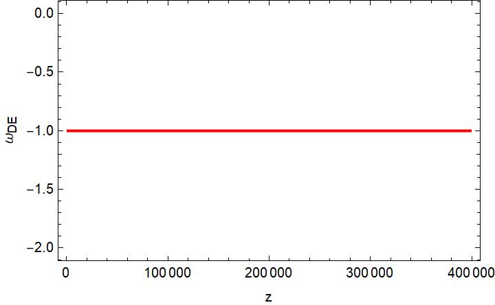
Figure 12: Dark energy EoS depending solely on redshift in the interval $z=[0,4\times 10^{5}]$. It becomes apparent that while the first remains constant as a direct consequence of the constant value if statefinder $y_{H}$, the latter remains infinitesimally close to zero and starts increasing for relatively small redshifts.

In subsequent models the numerical solutions will cover redshifts starting from present day at $z=0$ until the early radiation dominated era thus in the interval $[0,4\times 10^{5}]$. However before we proceed it is important to make a statement on the dimensionality of the initial condition of the derivative of the scalar field. Previously, it was given in terms of the Planck mass, which is indeed the case as function $\phi^{\prime}$ runs with eV. Note that the time derivative of the scalar field must have mass dimensions of eV² however due to the differential operator (133) which already runs with eV units, $\phi^{\prime}$ must also have the same exact units. As a final note, it should be stated that for the model at hand, it was assumed that perfect matter fluids were present therefore from Eq. (137) the dark energy density should also satisfy a perfect fluid continuity equation of the form,

$$\centering\dot{\rho}_{i}+3H\rho_{i}(1+\omega_{i})=0\,,\@add@centering$$ (146)

where index $i$ takes the values $m$, $r$ and $DE$ for non relativistic, relativistic and dark energy respectively. It should be stated that parameter $\omega_{i}$ characterizes the equation of state of each fluid, where for non relativistic matter $\omega_{m}=0$, for relativistic matter $\omega_{r}=\frac{1}{3}$. In the following, the EoS for dark energy shall be properly specified as a statefinder parameter and afterwards we shall ascertain whether for a given model compatible with Planck data [84], it is feasible to achieve a value of $\omega_{DE}\simeq-1$ at present day.

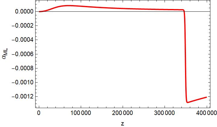
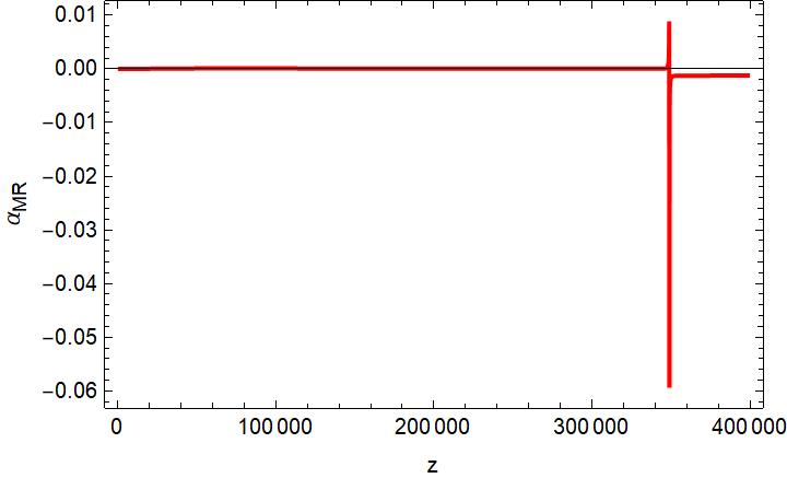
Figure 13: The behavior of the parameters $a_{ML}$ (left plot) and of $a_{MR}$ (right plot) for $z=[0,4\times 10^{5}]$.

In order properly study the late-time era and in general the validity of a particular model with the Planck data, and in particular the $\Lambda$CDM model, currently the best description of the Universe, certain statefinder parameters shall be extracted and in particular compared to such observable quantities. In the present article we shall limit our work to one statefinder parameter that specifies the evolution of the Universe and two that are solely connected to dark energy. In particular, we shall consider the deceleration parameter $q$, with regard to statefinders, and the dark energy EoS parameter $\omega_{DE}$, and the total EoS parameter $\omega_{tot}$. A proper description of the Universe admits a total EoS $\omega_{tot}$, which tends to $\omega_{tot}=-1$ for $z=0$, and tends asymptotically to $\omega_{tot}=\frac{1}{3}$ at approximately $z_{fin}=4\times 10^{5}$. Regarding dark energy, two statefinder parameters shall be studied, in particular the equation of state and the dark energy density parameter $\omega_{DE}$ and $\Omega_{DE}$ respectively which recall are given by the following expressions,

$$\centering\omega_{DE}\@add@centering =-1+\frac{1+z}{3}\frac{d\ln y_{H}}{dz} \Omega_{DE} =\frac{y_{H}}{y_{H}+\tilde{\rho}}\,,$$ (147)

In the following subsection we shall study the cosmological behavior of the model (101) from the dark energy era back to the early stages of the radiation domination era, and in some cases we shall compare the model with the $\Lambda$CDM model.

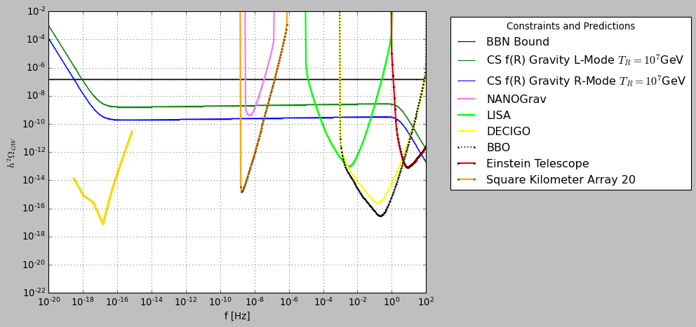
Figure 14: The $h^{2}$-scaled gravitational wave energy spectrum for the Chern-Simons corrected $k$-essence $f(R)$ gravity for the reheating temperature being $T_{R}=10^{7}$GeV.

III.4 Numerical Results

Let us quote here for reading convenience the analytic form of the model (101), which is,

$$\centering f(R)=R+\frac{R^{2}}{6M^{2}}-(R+R_{0})P_{3}\left(\frac{M_{P}^{2}}{R+R_{0}}\right)\,,\@add@centering$$ (148)

where by demanding compatibility with the Planck data, auxiliary parameters were specified as $M=1.25\cdot 10^{-5}\,M_{P}$, $\Lambda_{1}=4\cdot 10^{-12}$, $M_{1}=25\cdot 10^{-5.332}\Lambda_{1}\,M_{P}$. Also the $R_{0}$ serves as an effective mass scale which is assumed to be of order $R_{0}\sim 10^{-52}$eV². Finally the non-canonical parameter which participates in the $k$-essence contribution will be assumed to be related with the $e$-foldings number in the following way $f_{1}=2e^{N}$ with $N$ being $N=54.2$. Therefore, with these functions at hand and the numerical values of the auxiliary parameters, the equations of motion can be numerically solved and extract information about statefinder $y_{H}$ and the scalar field $\phi$ with respect to redshift. Now that such detail is out of the way, let us proceed directly to the numerical results of the aforementioned model.

We commence with the statefinders introduced previously that describe both the evolution of the Universe and the behavior of dark energy, which in this framework is identified as all the extra geometric terms participating in (100), coming both from the $f(R)$ and the $G(X)$ functions. Initially, for the solutions of equations (130) and (131) depicted in Fig 9, we find that the statefinder $y_{H}$ is stationary, as it was expected since the quantity $y_{H}$ is basically the dark energy density which in the case at hand behaves as a pure cosmological constant for the whole evolution of the Universe. Our numerical study presented in the left plot of Fig. 9 indicates this fact directly. In the right plot of Fig. 9 we present the behavior of the normalized scalar field as a function of the redshift, which decreases as the redshift approaches the present day value $z=0$. The fact that the statefinder $y_{H}$ as a solution is stable suggests that the evolution of Hubble’s parameter is solely specified by the component $\rho(z)$ but is shifted by an infinitesimal factor due to the contribution of the rest geometric terms, which indeed behave exactly as a cosmological constant, something which becomes abundantly clear subsequently. The fact that the initial conditions for the scalar field were positive imply that the late-era can indeed be smoothly connected to the inflationary era.

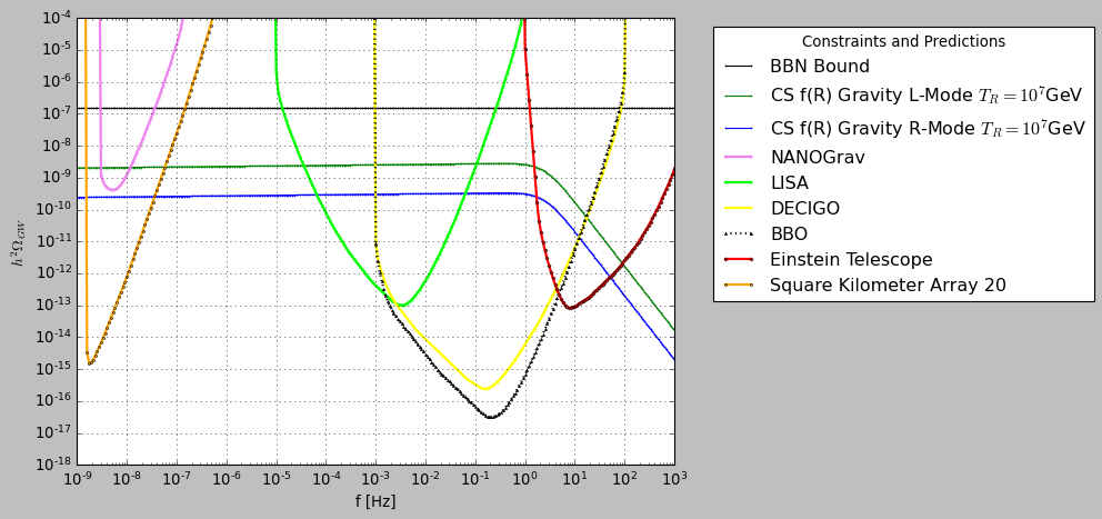
Figure 15: Close-up of the $h^{2}$-scaled gravitational wave energy spectrum for the Chern-Simons corrected $k$-essence $f(R)$ gravity for the reheating temperature being $T_{R}=10^{7}$GeV.

With regard to the deceleration parameter $q$ in Fig. 10 we plot its evolution as a function of the redshift (red curve), and it becomes apparent that the accelerating era is indeed compatible with latest observations. In the same plot, we also include the behavior of the deceleration parameter for the $\Lambda$CDM model. As it can be seen in Fig. 10, the model is indistinguishable from the $\Lambda$CDM model for the whole range of the redshift values $z=[0,4\times 10^{5}]$. In Table II we quote the values of the deceleration parameter at present day for the Chern-Simons $k$-essence $f(R)$ gravity and for the $\Lambda$CDM model. As shown, the deceleration parameter reaches the value of $q=-1$ in the future, with the current value also being negative and equal to $q=-0.52$ and furthermore reaches the value of $q=1$ for large values of redshift. Note that a numerical integration in the interval $[0,4\times 10^{5}]$ was performed so at order $z\sim 10^{3}$ one observes the deceleration parameter increasing with a relatively slow rate and going asymptotically to the value of $q=1$, meaning it transitions from the matter dominated era to the radiation dominated era smoothly as the redshift increases. Also in Fig. 11 we plot the behavior of the total EoS parameter as a function of the redshift. As expected it is quite close to zero during the matter dominated era, as it should, and starts increasing slowly towards the value of $\omega=\frac{1}{3}$ for $10^{3}<z<4\times 10^{5}$, for which interval, the numerical solution for $y_{H}$ and $\phi$ was extracted.

Table 2: Statefinders for the Chern-Simons $k$-essence $f(R)$ model compared to the $\Lambda$CDM Model.

Statefinder Parameter	k-essence $f(R)$ numerical value	$\Lambda$CDM Value
$q(0)$	-0.51895	-0.535
$\Omega_{DE}(0)$	0.679335	$0.6847\pm 0.0073$
$\omega_{DE}(0)$	-1	$-1.018\pm 0.031$

Finally, the dark energy EoS parameter as a function of the redshift is presented in Fig. 12, where it can be seen that $\omega_{DE}=-1$ for the whole range $z=[0,4\times 10^{5}]$ and this is no surprise since the dark energy behaves exactly as a cosmological constant. Thus the model is validated to mimic exactly the $\Lambda$CDM model.

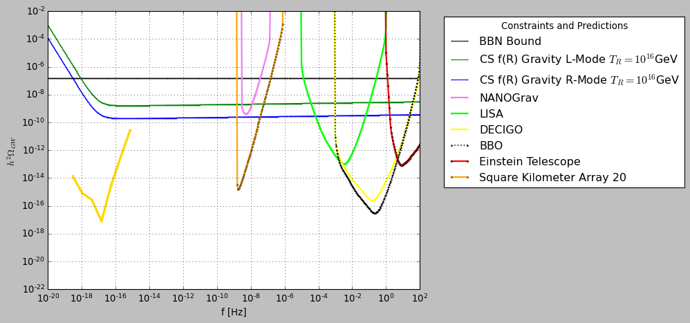
Figure 16: The $h^{2}$-scaled gravitational wave energy spectrum for the Chern-Simons corrected $k$-essence $f(R)$ gravity for the reheating temperature being $T_{R}=10^{16}$GeV.

Furthermore, for completeness in Table II we present the confrontation of the model with the 2018 Planck constraints [83] on the cosmological parameters or the comparison of the model with the $\Lambda$CDM model. As it can be seen, the model is compatible with the Planck data and mimics closely the $\Lambda$CDM model. Having the numerical solution for $y_{H}$ and effectively having the evolution of the Hubble rate available for the model at hand, makes the calculation of the parameters (60) easy and thus the “damping” factor $\mathcal{D}$ (50) and in effect $e^{-2\mathcal{D}}$, can be calculated directly for the Chern-Simons $k$-essence $f(R)$ gravity model. Having these available, the calculation of the primordial gravitational wave energy spectrum can be calculated easily. This is the subject of the next section.

III.5 Primordial Gravitational Wave Energy Spectrum

At this stage, after having solved the Friedmann equation numerically and having the numerical solution for the Hubble rate of the Chern-Simons $k$-essence $f(R)$ gravity model at hand, we can directly proceed in making predictions for the model’s primordial gravitational wave energy spectrum. Again, the spectrum will be evaluated by using the formula,

$$\Delta_{h}^{2}(k)=e^{-2\,\mathcal{D}}r\mathcal{P}_{\zeta}(k_{ref})\left(\frac{k}{k_{ref}}\right)^{n_{T}}\left(\frac{\Omega_{m}}{\Omega_{\Lambda}}\right)^{2}\left(\frac{g_{*}(T_{\rm in})}{g_{*0}}\right)\left(\frac{g_{*s0}}{g_{*s}(T_{\rm in})}\right)^{4/3}\left(\overline{\frac{3j_{1}(k\tau_{0})}{k\tau_{0}}}\right)^{2}T_{1}^{2}\left(x_{\rm eq}\right)T_{2}^{2}\left(x_{R}\right),$$ (149)

and recall that the primordial inflationary spectrum is evaluated at the CMB pivot scale $k_{ref}=0.002$ Mpc^-1, and the various parameters appearing in Eq. (149) are defined below Eq. (30). The “damping” factor $\mathcal{D}$ is evaluated by the formula (50) which for the Chern-Simons $k$-essence $f(R)$ gravity takes the form,

$$\mathcal{D}=\frac{1}{2}\int^{\tau}a_{M\ell}\mathcal{H}{\rm d}\tau_{1}=\frac{1}{2}\int_{0}^{z}\frac{a_{M\ell}}{1+z^{\prime}}{\rm dz^{\prime}}\,,$$ (150)

where recall that for redshifts $z=[0,4\times 10^{5}]$ the parameter $a_{M\ell}$ is given by,

$$a_{M\ell}=\frac{f_{RR}\dot{R}+2\lambda_{\ell}\ddot{\nu}k_{p}/a-2\lambda_{\ell}\dot{\nu}k_{p}H/a}{(f_{R}+2\lambda_{\ell}\dot{\nu}k_{p}/a)}\,,$$ (151)

where $k_{p}$ is the Chern-Simons pivot wavelength to be specified later on. For redshifts beyond $z\sim 4\times 10^{5}$, in which case the cosmological system has entered the radiation domination era, recall that the parameter $a_{M\ell}$ reads,

$$a_{M\ell}=\frac{2\lambda_{\ell}\ddot{\nu}k_{p}/a-2\lambda_{\ell}\dot{\nu}k_{p}H/a}{(f_{R}+2\lambda_{\ell}\dot{\nu}k_{p}/a)}\,.$$ (152)

since $\dot{R}\simeq 0$ for these redshifts. Now, having the formulas and the numerical solutions available we can proceed and make predictions for the primordial gravitational wave energy spectrum for the model at hand. We shall examine in detail how the primordial gravitational wave energy spectrum is affected by the $f(R)$, the $G(X)$ and the $\nu(\phi)$ functions, thus how does the $k$-essence and Chern-Simons terms affect the spectrum of the inflationary gravity waves today. It turns out that in general $G(X)$ is subleading compared to function $f(R)$, therefore one would expect an effective damping in the intensity of gravitational waves, which is typical for a plethora of $f(R)$ models. However, due to the inclusion of a Chern-Simons term and in particular the aforementioned toy model of an exponential scalar coupling function, one can easily evaluate such intensity for gravitational waves and come to the realization that the Chern-Simons term manages to enhance such signals up to $e^{-\mathcal{D}}\simeq 10^{9}$, thus the spectrum is amplified. Also due to the Chern-Simons term, the two polarization modes do not propagate equivalently, thus we end up with two distinct signals for the primordial gravitational waves. Let us analyze in detail the physical picture, so for the exponential Chern-Simons coupling of Eq. (129), and the numerical solution for the Hubble rate $H(z)$ in Fig. 13 we plot the behavior of the parameters $a_{ML}$ (left plot) and of $a_{MR}$ (right plot) for $z=[0,4\times 10^{5}]$.

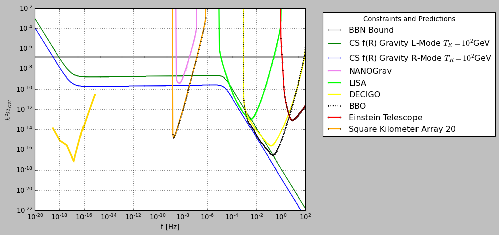
Figure 17: The $h^{2}$-scaled gravitational wave energy spectrum for the Chern-Simons corrected $k$-essence $f(R)$ gravity for the reheating temperature being $T_{R}=10^{2}$GeV.

As it is obvious, firstly the contribution of both the modes will lead to an overall amplification of the primordial gravitational wave signal and secondly the two polarizations lead to a different value of amplification. By computing the “damping” factor for the two polarization modes, we get $e^{-2\mathcal{D}_{L}}\simeq 7.0267\times 10^{9}$ and $e^{-2\mathcal{D}_{R}}=8.42676\times 10^{8}$, and note that for the evaluation of the integral we used a Chern-Simons pivot wavelength of the order $k_{p}\sim 10^{11}$ Mpc^-1 which comparable to the wavelengths of the modes that crossed the horizon for the second time around the reheating era, and for modes related to the LISA, DECIGO, BBO and Einstein Telescope. Thus the amplification of the gravitational wave signal is apparent, and also the two polarizations lead to different amplifications, thus two signals are expected and this is indeed what happens. Also our analysis indicated that the reheating temperature also affects the energy spectrum of the primordial gravitational waves, as expected from the related literature [43]. In Figs. 14 and 15 we plot the primordial gravitational wave energy spectrum for reheating temperature $T_{R}=10^{7}$GeV, actually Fig. 15 is a close up of Fig. 14. Also in Figs. 16 and 17 the primordial gravitational wave energy spectrum is plotted for the reheating temperature chosen $T_{R}=10^{16}$GeV and $T_{R}=10^{2}$GeV respectively. We need to note that for all the gravitational wave spectrum calculations, the tensor spectral index was chosen $n_{T}=0.0165879$ and the tensor-to-scalar ratio $r=0.00316538$ and these values were obtained in the section where the inflationary era was discussed for the $k$-essence $f(R)$ gravity model with exponential Chern-Simons coupling.

At this point let us discuss the resulting physical picture, which seems quite intriguing. Firstly, the gravitational wave spectrum signal for the Chern-Simons $k$-essence $f(R)$ gravity model at hand is detectable by almost all the future collaborations, and for all the reheating temperatures, except when $T_{R}=10^{2}$GeV in which case the Einstein Telescope will not capture any signal for this particular model. Secondly, this specific model, due to the Chern-Simons coupling and the inequivalent propagation of the two polarization modes, leads to two distinct signals, which is a possibility that one could expect in future experiments like the LISA collaboration etc. Furthermore, the reheating temperature also affects the spectrum, a feature which was also expected. Finally, for the model at hand, the BBN bound (62) is violated only for modes that reentered the horizon quite “close” to present time, for frequencies below $10^{-18}$Hz. In fact at this frequency range, only the LiteBird may detect signals up to $10^{-18}$Hz, but for the model at hand, as we already mentioned, below $10^{-18}$Hz the model violates the BBN bound. This effect however might be due to the fact that we did not take into account the damping effect caused in the spectrum by neutrino and other relativistic particles freestreaming below $f\sim 10^{-15}$Hz, which could lower significantly the gravitational wave energy spectrum of the model at hand. In any case this is a toy-pedagogical model that we use in order to extract useful information for the predictions of modified gravity gravitational waves energy spectrum for frequencies probed by LISA and other experiments of the same frequency band, so we do not aim to focus on low frequencies. The resulting picture by combining the results of this section and the results of the pure $f(R)$ gravity section, is quite interesting since simply stated, the plot thickens with future observations. Simple $f(R)$ gravity models cannot lead to detectable primordial gravitational waves, however, exotic terms like the Chern-Simons, may generate a detectable signal by some or all the collaborations. This feature is mainly controlled by the tensor spectral index. A positive tensor spectral index, combined with a reasonable value of the tensor-to-scalar ratio, will surely be detected by some or all the future experiments. A negative tensor spectral index will possibly lead to a non-detectable primordial gravitational wave energy spectrum signal. Also, one may indirectly determine, or obtain useful information for, the reheating temperature. This however might be a model-dependent feature to our opinion. Thus what should one expect by the detection or the non-detection of the primordial gravitational waves in future experiments? We list here some of the most important features:

• No signal is detected in future experiments. Bad news for inflation? Not necessarily. If the sensitivities of the experiments like LISA are higher than the signal, one cannot exclude scalar models or modified gravity models like $f(R)$ gravity. One is sure in this case, the tensor spectral index is negative, and no conclusion can be made for the reheating temperature.

• A signal is detected in some or all the future experiments. Then one may conclude that a positive tensor spectral index is the characteristic of the underlying theory. Since the single scalar field theory can yield a blue-tilted tensor spectral index only when it is a tachyonic theory, a possible detection of a primordial gravitational wave signal will exclude single field inflation possibly. The reheating temperature is a model dependent feature, so by combining results from different experiments, one may conclude if it is smaller than, or larger than $T_{R}=10^{7}$GeV. Now depending on the magnitude of the observed spectrum, compared to the GR result with a positive tensor spectral index, is it possible to conclude whether a modified gravity drives the evolution? Possibly no, there are models which we shall present elsewhere, for which the spectrum is identical with the GR spectrum with blue-tilted tensor spectral index.

Thus in conclusion, the plot thickens with primordial gravitational waves in future observational missions and experiments. Modified gravity blurs the outcomes to say the least. The signal is affected mainly from the tensor spectral index and the reheating temperature only in this case, but no one can say for sure which modified gravity drives the evolution. Certainly though if a signal is detected, a non-conventional modified gravity of some sort must be generating the signal, with a positive tensor spectral index. If no signal is detected, things will be as they are now, and the question whether inflation took ever place cannot be answered unless the sensitivities are improved in the far future. If in the far future, no signal is detected again, then possibly inflation must be abandoned as a candidate for describing the primordial era of our Universe.

IV Future Perspectives and Concluding Remarks

In this work we addressed in a quantitative way the primordial gravitational wave problem in the context of $f(R)$ gravity related theories. We chose the $f(R)$ gravity models in such a way so that both inflation and dark energy can be described in a unified way. Actually for both the models, all the cosmological eras can be described in a viable way, that is from inflation a smooth transition is guaranteed to the radiation era, which gradually evolves to the matter domination era, and the latter smoothly evolves to the dark energy era. Also both the models we used, mimic the $\Lambda$CDM model at late times, and one of the two models is indistinguishable from the $\Lambda$CDM model from the dark energy back to the radiation domination era. Both the models studied produce a viable inflationary era which is compatible with the Planck 2018 constraints on inflation, and both the models are also compatible with the 2018 cosmological constraints of the Planck collaboration. We used a WKB formalism in order to quantify the effect of the modified gravity models and we arranged the cosmological equations in such a way so that to facilitate the calculation of the WKB contribution to the primordial gravitational wave waveform. For the pure $f(R)$ gravity model, the primordial gravitational wave energy spectrum was slightly enhanced compared to the GR spectrum, however the predicted spectrum was way below the lowest sensitivities of the future experiments at large frequencies. This feature has as source the red-tilted tensor spectral index of the pure $f(R)$ gravity and in order to investigate what would happen in the case that a blue tensor spectral index was produced, we provided a Chern-Simons potential-less $k$-essence $f(R)$ gravity model, which as we showed can produce a blue-tilted tensor spectral index. After calculating the predicted energy spectrum of the primordial gravitational waves, we demonstrated that this model has two interesting features, firstly the presence of two signals of primordial gravitational waves, and secondly the spectrum is significantly enhanced compared to GR, thus it can be detected from all the future experiments on gravitational waves. Another interesting feature is that the reheating temperature affects the energy spectrum of the gravitational waves, and actually for low-reheating temperatures, at high frequencies the energy spectrum of the gravitational waves drops significantly, and in some cases, it ceases to be detectable from the future experiments, like for example from the Einstein telescope.

Also we discussed the possibility of signal detection, or the absence of a stochastic signal detection in future experiments, and what would these situations mean for inflation. If no signal is detected would this mean the end of inflation? Possibly no, since a red-tilted spectral index would be produced from a scalar or some other theory, and the signal might lie below the lower sensitivities of the future experiments. So even more sensitive future experiments would be required in order to conclude whether inflation ever took place. So in the case of no signal detection in all future experiments, the following conclusions can be reached probably:

• Inflation might still be a valid theory for the primordial era.

• A single scalar field theory, or a pure $f(R)$ gravity or any other theory that can produce a red-tilted tensor spectral index might actually be responsible for the inflationary era.

• The tensor spectral index of the primordial tensor perturbations is probably red-tilted.

If in some future experiments a signal is detected, or if the signal is detected in all the experiments, then the following conclusions can be made:

• The tensor spectral index is definitely positive.

• Single field inflation is excluded, because tachyon inflation is bad news for physics.

• An exotic modified gravity that can produce a blue-tilted tensor spectral index, certainly drives inflation, perhaps in combination with some scalar field theory.

• Depending on the detected signal, conclusions on the reheating temperature can be made, especially if the signal is detected in some future experiments, in a specific frequency range, and not in another frequency range.

• If the signal is detected in some but not all the future experiments, we may seek for further suppression mechanisms in the frequencies that no detection occurs. Perhaps another mechanism further suppresses the energy spectrum of the primordial gravitational waves in a specific frequency range, for example supersymmetry breaking. This is a rather exciting perspective.

• Depending on the magnitude of the signal, one may even try to narrow down the modified gravity theories that may produce such spectrum. For example, as we will report in some time from now, Einstein-Gauss-Bonnet theories do not enhance the signal, but produce a blue-tilted tensor spectral index. Thus one may theorize whether a stringy theory drives inflation or inflation is driven by some more involved modified gravity, like the Chern-Simons $k$-essence $f(R)$ gravity we presented in this paper.

• If two signals are detected, then the presence of Chern-Simons term is guaranteed to be present during the inflationary era.

Thus in conclusion, as it was expected, the detection of a signal in future experiments will put the theoretical minds into fire, trying to pinpoint the underlying theory that is observed in the experiments. This perspective is exciting and we surely hope that this might be the case in the future. Such a result would indicate that single scalar field inflation might be assisted, not solely by curvature terms [90], but also by more exotic terms, like the Chern-Simons terms. In the case of detection of signals, cosmologists are confronted with a demanding challenge: the models that they use thereafter must provide a unified description of dark energy and inflation, with a smooth transition in between them, passing through the radiation and matter domination eras, a successful late and inflationary phenomenology, and the model must also produce the right amount of gravitational radiation in order to comply with the future detected signals. Exciting and demanding perspective to say the least. In this work we tried to provide the first models toward this direction.

To conclude, there are further possibilities for model building that we did not take into account, like for example the possibility of having a model with blue-tilted tensor spectral index that can produce an early dark energy era [14]. This kind of models could also simultaneously provide insights for alleviating the Hubble tension problem, but we refrain to go deeply in these problems unless the calibration issues [79, 80] of the Hubble tension observations are appropriately resolved. In the same spirit, a possible deviation from a pure radiation domination era occurring prior to the BBN, can be directly impacted and spotted on the gravitational wave energy spectrum, for large frequencies, larger than $f>10^{-11}$Hz. In this case, the phenomenology is quite rich, even in the context of pure $f(R)$ gravity, a problem that we will report in due time. A last interesting perspective that is worthy mentioning is the effect of primordial non-Gaussianities on gravitational waves, or the induction of gravitational wave by the non-Gaussianities see for example [91], and this issue is also worthy studying in a future work.

References

- [1] A. D. Linde, Lect. Notes Phys. 738 (2008) 1 [arXiv:0705.0164 [hep-th]].
- [2] D. S. Gorbunov and V. A. Rubakov, “Introduction to the theory of the early universe: Cosmological perturbations and inflationary theory,” Hackensack, USA: World Scientific (2011) 489 p;
- [3] A. Linde, arXiv:1402.0526 [hep-th];
- [4] D. H. Lyth and A. Riotto, Phys. Rept. 314 (1999) 1 [hep-ph/9807278].
- [5] M. Kamionkowski and E. D. Kovetz, Ann. Rev. Astron. Astrophys. 54 (2016) 227 doi:10.1146/annurev-astro-081915-023433 [arXiv:1510.06042 [astro-ph.CO]].
- [6] M. Denissenya and E. V. Linder, JCAP 11 (2018), 010 doi:10.1088/1475-7516/2018/11/010 [arXiv:1808.00013 [astro-ph.CO]].
- [7] M. S. Turner, M. J. White and J. E. Lidsey, Phys. Rev. D 48 (1993), 4613-4622 doi:10.1103/PhysRevD.48.4613 [arXiv:astro-ph/9306029 [astro-ph]].
- [8] L. A. Boyle and P. J. Steinhardt, Phys. Rev. D 77 (2008), 063504 doi:10.1103/PhysRevD.77.063504 [arXiv:astro-ph/0512014 [astro-ph]].
- [9] B. F. Schutz and F. Ricci, [arXiv:1005.4735 [gr-qc]].
- [10] B. S. Sathyaprakash and B. F. Schutz, Living Rev. Rel. 12 (2009), 2 doi:10.12942/lrr-2009-2 [arXiv:0903.0338 [gr-qc]].
- [11] C. Caprini and D. G. Figueroa, Class. Quant. Grav. 35 (2018) no.16, 163001 doi:10.1088/1361-6382/aac608 [arXiv:1801.04268 [astro-ph.CO]].
- [12] G. Arutyunov, M. Heinze and D. Medina-Rincon, J. Phys. A 50 (2017) no.24, 244002 doi:10.1088/1751-8121/aa6e0c [arXiv:1608.06481 [hep-th]].
- [13] S. Kuroyanagi, T. Chiba and N. Sugiyama, Phys. Rev. D 79 (2009), 103501 doi:10.1103/PhysRevD.79.103501 [arXiv:0804.3249 [astro-ph]].
- [14] T. J. Clarke, E. J. Copeland and A. Moss, JCAP 10 (2020), 002 doi:10.1088/1475-7516/2020/10/002 [arXiv:2004.11396 [astro-ph.CO]].
- [15] S. Kuroyanagi, T. Takahashi and S. Yokoyama, JCAP 02 (2015), 003 doi:10.1088/1475-7516/2015/02/003 [arXiv:1407.4785 [astro-ph.CO]].
- [16] K. Nakayama and J. Yokoyama, JCAP 01 (2010), 010 doi:10.1088/1475-7516/2010/01/010 [arXiv:0910.0715 [astro-ph.CO]].
- [17] T. L. Smith, M. Kamionkowski and A. Cooray, Phys. Rev. D 73 (2006), 023504 doi:10.1103/PhysRevD.73.023504 [arXiv:astro-ph/0506422 [astro-ph]].
- [18] M. Giovannini, Class. Quant. Grav. 26 (2009), 045004 doi:10.1088/0264-9381/26/4/045004 [arXiv:0807.4317 [astro-ph]].
- [19] X. J. Liu, W. Zhao, Y. Zhang and Z. H. Zhu, Phys. Rev. D 93 (2016) no.2, 024031 doi:10.1103/PhysRevD.93.024031 [arXiv:1509.03524 [astro-ph.CO]].
- [20] W. Zhao, Y. Zhang, X. P. You and Z. H. Zhu, Phys. Rev. D 87 (2013) no.12, 124012 doi:10.1103/PhysRevD.87.124012 [arXiv:1303.6718 [astro-ph.CO]].
- [21] S. Vagnozzi, Mon. Not. Roy. Astron. Soc. 502 (2021) no.1, L11-L15 doi:10.1093/mnrasl/slaa203 [arXiv:2009.13432 [astro-ph.CO]].
- [22] Y. Watanabe and E. Komatsu, Phys. Rev. D 73 (2006), 123515 doi:10.1103/PhysRevD.73.123515 [arXiv:astro-ph/0604176 [astro-ph]].
- [23] M. Kamionkowski, A. Kosowsky and M. S. Turner, Phys. Rev. D 49 (1994), 2837-2851 doi:10.1103/PhysRevD.49.2837 [arXiv:astro-ph/9310044 [astro-ph]].
- [24] W. Giarè and F. Renzi, Phys. Rev. D 102 (2020) no.8, 083530 doi:10.1103/PhysRevD.102.083530 [arXiv:2007.04256 [astro-ph.CO]].
- [25] S. Kuroyanagi, T. Takahashi and S. Yokoyama, JCAP 01 (2021), 071 doi:10.1088/1475-7516/2021/01/071 [arXiv:2011.03323 [astro-ph.CO]].
- [26] W. Zhao and Y. Zhang, Phys. Rev. D 74 (2006), 043503 doi:10.1103/PhysRevD.74.043503 [arXiv:astro-ph/0604458 [astro-ph]].
- [27] A. Nishizawa, Phys. Rev. D 97 (2018) no.10, 104037 doi:10.1103/PhysRevD.97.104037 [arXiv:1710.04825 [gr-qc]].
- [28] S. Arai and A. Nishizawa, Phys. Rev. D 97 (2018) no.10, 104038 doi:10.1103/PhysRevD.97.104038 [arXiv:1711.03776 [gr-qc]].
- [29] E. Bellini and I. Sawicki, JCAP 07 (2014), 050 doi:10.1088/1475-7516/2014/07/050 [arXiv:1404.3713 [astro-ph.CO]].
- [30] R. C. Nunes, M. E. S. Alves and J. C. N. de Araujo, Phys. Rev. D 99 (2019) no.8, 084022 doi:10.1103/PhysRevD.99.084022 [arXiv:1811.12760 [gr-qc]].
- [31] R. D’Agostino and R. C. Nunes, Phys. Rev. D 100 (2019) no.4, 044041 doi:10.1103/PhysRevD.100.044041 [arXiv:1907.05516 [gr-qc]].
- [32] A. Mitra, J. Mifsud, D. F. Mota and D. Parkinson, Mon. Not. Roy. Astron. Soc. 502 (2021) no.4, 5563-5575 doi:10.1093/mnras/stab165 [arXiv:2010.00189 [astro-ph.CO]].
- [33] S. Kuroyanagi, K. Nakayama and S. Saito, Phys. Rev. D 84 (2011), 123513 doi:10.1103/PhysRevD.84.123513 [arXiv:1110.4169 [astro-ph.CO]].
- [34] P. Campeti, E. Komatsu, D. Poletti and C. Baccigalupi, JCAP 01 (2021), 012 doi:10.1088/1475-7516/2021/01/012 [arXiv:2007.04241 [astro-ph.CO]].
- [35] A. Nishizawa and H. Motohashi, Phys. Rev. D 89 (2014) no.6, 063541 doi:10.1103/PhysRevD.89.063541 [arXiv:1401.1023 [astro-ph.CO]].
- [36] W. Zhao, Chin. Phys. 16 (2007), 2894-2902 doi:10.1088/1009-1963/16/10/012 [arXiv:gr-qc/0612041 [gr-qc]].
- [37] W. Cheng, T. Qian, Q. Yu, H. Zhou and R. Y. Zhou, [arXiv:2107.04242 [hep-ph]].
- [38] A. Nishizawa, K. Yagi, A. Taruya and T. Tanaka, Phys. Rev. D 85 (2012), 044047 doi:10.1103/PhysRevD.85.044047 [arXiv:1110.2865 [astro-ph.CO]].
- [39] S. Chongchitnan and G. Efstathiou, Phys. Rev. D 73 (2006), 083511 doi:10.1103/PhysRevD.73.083511 [arXiv:astro-ph/0602594 [astro-ph]].
- [40] P. D. Lasky, C. M. F. Mingarelli, T. L. Smith, J. T. Giblin, D. J. Reardon, R. Caldwell, M. Bailes, N. D. R. Bhat, S. Burke-Spolaor and W. Coles, et al. Phys. Rev. X 6 (2016) no.1, 011035 doi:10.1103/PhysRevX.6.011035 [arXiv:1511.05994 [astro-ph.CO]].
- [41] M. C. Guzzetti, N. Bartolo, M. Liguori and S. Matarrese, Riv. Nuovo Cim. 39 (2016) no.9, 399-495 doi:10.1393/ncr/i2016-10127-1 [arXiv:1605.01615 [astro-ph.CO]].
- [42] I. Ben-Dayan, B. Keating, D. Leon and I. Wolfson, JCAP 06 (2019), 007 doi:10.1088/1475-7516/2019/06/007 [arXiv:1903.11843 [astro-ph.CO]].
- [43] K. Nakayama, S. Saito, Y. Suwa and J. Yokoyama, JCAP 06 (2008), 020 doi:10.1088/1475-7516/2008/06/020 [arXiv:0804.1827 [astro-ph]].
- [44] S. Capozziello, M. De Laurentis, S. Nojiri and S. D. Odintsov, Phys. Rev. D 95 (2017) no.8, 083524 doi:10.1103/PhysRevD.95.083524 [arXiv:1702.05517 [gr-qc]].
- [45] S. Capozziello, M. De Laurentis, S. Nojiri and S. D. Odintsov, Gen. Rel. Grav. 41 (2009), 2313-2344 doi:10.1007/s10714-009-0758-1 [arXiv:0808.1335 [hep-th]].
- [46] S. Capozziello, C. Corda and M. F. De Laurentis, Phys. Lett. B 669 (2008), 255-259 doi:10.1016/j.physletb.2008.10.001 [arXiv:0812.2272 [astro-ph]].
- [47] R. G. Cai, C. Fu and W. W. Yu, [arXiv:2112.04794 [astro-ph.CO]].
- [48] S. Hild, M. Abernathy, F. Acernese, P. Amaro-Seoane, N. Andersson, K. Arun, F. Barone, B. Barr, M. Barsuglia and M. Beker, et al. Class. Quant. Grav. 28 (2011), 094013 doi:10.1088/0264-9381/28/9/094013 [arXiv:1012.0908 [gr-qc]].
- [49] J. Baker, J. Bellovary, P. L. Bender, E. Berti, R. Caldwell, J. Camp, J. W. Conklin, N. Cornish, C. Cutler and R. DeRosa, et al. [arXiv:1907.06482 [astro-ph.IM]].
- [50] T. L. Smith and R. Caldwell, Phys. Rev. D 100 (2019) no.10, 104055 doi:10.1103/PhysRevD.100.104055 [arXiv:1908.00546 [astro-ph.CO]].
- [51] J. Crowder and N. J. Cornish, Phys. Rev. D 72 (2005), 083005 doi:10.1103/PhysRevD.72.083005 [arXiv:gr-qc/0506015 [gr-qc]].
- [52] T. L. Smith and R. Caldwell, Phys. Rev. D 95 (2017) no.4, 044036 doi:10.1103/PhysRevD.95.044036 [arXiv:1609.05901 [gr-qc]].
- [53] N. Seto, S. Kawamura and T. Nakamura, Phys. Rev. Lett. 87 (2001), 221103 doi:10.1103/PhysRevLett.87.221103 [arXiv:astro-ph/0108011 [astro-ph]].
- [54] S. Kawamura, M. Ando, N. Seto, S. Sato, M. Musha, I. Kawano, J. Yokoyama, T. Tanaka, K. Ioka and T. Akutsu, et al. [arXiv:2006.13545 [gr-qc]].
- [55] A. Weltman, P. Bull, S. Camera, K. Kelley, H. Padmanabhan, J. Pritchard, A. Raccanelli, S. Riemer-Sørensen, L. Shao and S. Andrianomena, et al. Publ. Astron. Soc. Austral. 37 (2020), e002 doi:10.1017/pasa.2019.42 [arXiv:1810.02680 [astro-ph.CO]].
- [56] Z. Arzoumanian et al. [NANOGrav], Astrophys. J. Lett. 905 (2020) no.2, L34 doi:10.3847/2041-8213/abd401 [arXiv:2009.04496 [astro-ph.HE]].
- [57] N. S. Pol et al. [NANOGrav], [arXiv:2010.11950 [astro-ph.HE]].
- [58] C. Vafa, hep-th/0509212.
- [59] H. Ooguri and C. Vafa, Nucl. Phys. B 766 (2007) 21 doi:10.1016/j.nuclphysb.2006.10.033 [hep-th/0605264].
- [60] E. Palti, C. Vafa and T. Weigand, arXiv:2003.10452 [hep-th].
- [61] S. D. Odintsov and V. K. Oikonomou, Phys. Lett. B 805 (2020), 135437 doi:10.1016/j.physletb.2020.135437 [arXiv:2004.00479 [gr-qc]].
- [62] S. Nojiri, S. D. Odintsov and V. K. Oikonomou, Phys. Rept. 692 (2017) 1 [arXiv:1705.11098 [gr-qc]].
-
[63]
S. Capozziello, M. De Laurentis,
Phys. Rept. 509, 167 (2011);
V. Faraoni and S. Capozziello, Fundam. Theor. Phys. 170 (2010). - [64] S. Nojiri, S.D. Odintsov, eConf C0602061, 06 (2006) [Int. J. Geom. Meth. Mod. Phys. 4, 115 (2007)].
- [65] S. Nojiri, S.D. Odintsov, Phys. Rept. 505, 59 (2011);
- [66] A. de la Cruz-Dombriz and D. Saez-Gomez, Entropy 14 (2012) 1717 [arXiv:1207.2663 [gr-qc]].
- [67] G. J. Olmo, Int. J. Mod. Phys. D 20 (2011) 413 [arXiv:1101.3864 [gr-qc]].
- [68] S. Nojiri and S. D. Odintsov, Phys. Rev. D 68 (2003) 123512 doi:10.1103/PhysRevD.68.123512 [hep-th/0307288].
- [69] S. Nojiri and S. D. Odintsov, Phys. Lett. B 657 (2007) 238 doi:10.1016/j.physletb.2007.10.027 [arXiv:0707.1941 [hep-th]].
- [70] S. Nojiri and S. D. Odintsov, Phys. Rev. D 77 (2008) 026007 doi:10.1103/PhysRevD.77.026007 [arXiv:0710.1738 [hep-th]].
- [71] G. Cognola, E. Elizalde, S. Nojiri, S. D. Odintsov, L. Sebastiani and S. Zerbini, Phys. Rev. D 77 (2008) 046009 doi:10.1103/PhysRevD.77.046009 [arXiv:0712.4017 [hep-th]].
- [72] S. Nojiri and S. D. Odintsov, Phys. Rev. D 74 (2006) 086005 doi:10.1103/PhysRevD.74.086005 [hep-th/0608008].
- [73] S. A. Appleby and R. A. Battye, Phys. Lett. B 654 (2007) 7 doi:10.1016/j.physletb.2007.08.037 [arXiv:0705.3199 [astro-ph]].
- [74] E. Elizalde, S. Nojiri, S. D. Odintsov, L. Sebastiani and S. Zerbini, Phys. Rev. D 83 (2011) 086006 doi:10.1103/PhysRevD.83.086006 [arXiv:1012.2280 [hep-th]].
- [75] S. D. Odintsov and V. K. Oikonomou, arXiv:2001.06830 [gr-qc].
- [76] V. K. Oikonomou, Phys. Rev. D 103 (2021) no.4, 044036 doi:10.1103/PhysRevD.103.044036 [arXiv:2012.00586 [astro-ph.CO]].
- [77] V. K. Oikonomou, [arXiv:2012.01312 [gr-qc]].
- [78] M. Breitbach, J. Kopp, E. Madge, T. Opferkuch and P. Schwaller, JCAP 07 (2019), 007 doi:10.1088/1475-7516/2019/07/007 [arXiv:1811.11175 [hep-ph]].
- [79] E. Mortsell, A. Goobar, J. Johansson and S. Dhawan, [arXiv:2105.11461 [astro-ph.CO]].
- [80] L. Perivolaropoulos and F. Skara, [arXiv:2109.04406 [astro-ph.CO]].
- [81] J. c. Hwang and H. Noh, Phys. Rev. D 71 (2005) 063536 doi:10.1103/PhysRevD.71.063536 [gr-qc/0412126].
- [82] J. Garcia-Bellido, [arXiv:hep-ph/0004188 [hep-ph]].
- [83] Y. Akrami et al. [Planck Collaboration], arXiv:1807.06211 [astro-ph.CO].
- [84] N. Aghanim et al. [Planck Collaboration], arXiv:1807.06209 [astro-ph.CO].
- [85] S. A. Appleby, R. A. Battye and A. A. Starobinsky, JCAP 1006 (2010) 005 [arXiv:0909.1737 [astro-ph.CO]].
- [86] S. D. Odintsov and V. K. Oikonomou, Phys. Lett. B 807 (2020), 135576 doi:10.1016/j.physletb.2020.135576 [arXiv:2005.12804 [gr-qc]].
- [87] K. Bamba, A. Lopez-Revelles, R. Myrzakulov, S. D. Odintsov and L. Sebastiani, Class. Quant. Grav. 30 (2013), 015008 doi:10.1088/0264-9381/30/1/015008 [arXiv:1207.1009 [gr-qc]].
- [88] M. Benetti and S. Capozziello, arXiv:1910.09975 [astro-ph.CO].
- [89] S. Nojiri, S. D. Odintsov and V. K. Oikonomou, Nucl. Phys. B 941 (2019), 11-27 doi:10.1016/j.nuclphysb.2019.02.008 [arXiv:1902.03669 [gr-qc]].
- [90] V. K. Oikonomou, Annals Phys. 432 (2021), 168576 doi:10.1016/j.aop.2021.168576 [arXiv:2108.04050 [gr-qc]].
- [91] R. g. Cai, S. Pi and M. Sasaki, Phys. Rev. Lett. 122 (2019) no.20, 201101 doi:10.1103/PhysRevLett.122.201101 [arXiv:1810.11000 [astro-ph.CO]].