Stochastic Variational Approach to Small Atoms and Molecules Coupled to Quantum Field Modes
Abstract
In this work, we present a stochastic variational calculation (SVM) of energies and wave functions of few particle systems coupled to quantum fields in cavity QED. The light-matter coupled system is described by the Pauli–Fierz Hamiltonian. The spatial wave function and the photon spaces are optimized by a random selection process. Examples for a two-dimensional trion and confined electrons as well as for the He atom and the H2 molecule are presented showing that the light-matter coupling drastically changes the electronic states.
Strong coupling of cavity electromagnetic modes and molecules create hybrid light-matter states that combine the properties of their ingredients modifying potential energy surfaces, charge states, and electronic structure. The possibility of altering physical and chemical properties by coupling to light attracted intense experimental Feist and Garcia-Vidal (2015); Balili et al. (2007); Schachenmayer et al. (2015); Xiang et al. (2020); Reserbat-Plantey et al. (2021); Coles et al. (2014); Kasprzak et al. (2006); Schwartz et al. (2011); Plumhof et al. (2014); Hutchison et al. (2013); Wang et al. (2021a); Basov et al. (2021) and theoretical interestMazza and Georges (2019); Di Stefano et al. (2019); Galego et al. (2015); Herrera and Spano (2016); Galego et al. (2016); Shalabney et al. (2015); Buchholz et al. (2019); Schäfer et al. (2019); Ruggenthaler et al. (2018); Flick et al. (2015, 2017); Lacombe et al. (2019); Mandal et al. (2020a); Flick et al. (2019); Latini et al. (2019); Flick et al. (2018a); Flick and Narang (2018); Garcia-Vidal et al. (2021); Thomas et al. (2019); Mordovina et al. (2020); Wang et al. (2021b); DePrince (2021); Haugland et al. (2021); Hoffmann et al. (2020); Flick and Narang (2020); Mandal et al. (2020b); Galego et al. (2017); Hoffmann et al. (2020); Flick et al. (2015, 2018b); Schafer et al. (2018); Sidler et al. (2020); Theophilou et al. (2020); Sidler et al. (2021); Buchholz et al. (2020); Tokatly (2018); Rivera et al. (2019); Szidarovszky et al. (2020); Cederbaum (2021). The experimental investigations are overarching exciton transport Feist and Garcia-Vidal (2015); Schachenmayer et al. (2015), polariton condensation Balili et al. (2007); Plumhof et al. (2014), transfer of excitation Coles et al. (2014), and chemical reactivity Thomas et al. (2016). The theoretical works explored excitation and charge transfer Schäfer et al. (2019), self-polarization Hoffmann et al. (2020), potential energy surfaces Lacombe et al. (2019) electron transfer Mandal et al. (2020b), excitons Latini et al. (2019), ionization potentials DePrince (2021), and intermolecular interactions Haugland et al. (2021) in cavities, to name a few.
For atoms and molecules in a vacuum, high precision measurements and theoretical calculations have been developed. For example, the accuracy of theoretical prediction Puchalski et al. (2019) and experimental measurement Hölsch et al. (2019) reaches the level of 1 MHz for the dissociation energy of the H2 molecule. The theoretical description of the light-matter hybrid states is far from this accuracy. The main reason behind this is that the accurate wave function methods developed in quantum chemistry are tedious and computationally expensive even before an additional degree of freedom (light) is added, and the density functional theory Kohn and Sham (1965) calculations lack suitable exchange correlation functionals for light-matter coupling. Initial developments have been started in both directions Buchholz et al. (2019); Flick et al. (2015, 2019); Mordovina et al. (2020); DePrince (2021); Flick and Narang (2020).
In this work, we use the stochastic variational method to build optimized light-matter coupled wave functions. The calculations can reach the same accuracy as conventional high precision calculations for small systems. We will show that the light-matter coupled wave functions are drastically different from the non-coupled electronic wave functions and the wave functions belonging to different photon spaces are very dissimilar (requiring separate optimizations).
The spatial wave functions will be represented by Explicitly Correlated Gaussian (ECG) basis functions Mitroy et al. (2013). The advantage of the approach is that the matrix elements are analytically available Suzuki et al. (1998); Cioslowski and Strasburger (2017); Zaklama et al. (2019) and it allows very accurate calculations of energies and wave functions Mitroy et al. (2013); Zhang et al. (2015); Kidd et al. (2016); Riva et al. (2000); Varga (1999); Usukura et al. (1999); Varga et al. (2001).
We assume that the system is nonrelativistic and the coupling to the light can be described by the dipole approximation. The Pauli-Fierz (PF) non-relativistic QED Hamiltonian provides a consistent quantum description at this level Ruggenthaler et al. (2018); Rokaj et al. (2018); Mandal et al. (2020a, b); Tokatly (2018). The PF Hamiltonian in the Coulomb gauge is where is the electronic Hamiltonian and
| (1) |
(atomic units are used in this work). In Eq. (1) is the dipole operator, the photon fields are described by quantized oscillators, and is the displacement field. This Hamiltonian describes photon modes with photon frequency and coupling . The coupling term is usually written as Ruggenthaler et al. (2014) , where is the cavity mode function at position and is the transversal polarization vector of the photon modes. The first term in Eq. (1) is the Hamiltonian of the photon modes, the second term couples the photons to the dipole, and the last term is the dipole self-interaction, .
The Hamiltonian of an electron system interacting with a Coulomb interaction and confined in an external potential reads as
| (2) |
where , and are the coordinate, charge, and mass of the th particle ( for electrons in atomic units).
Introducing the shorthand notations , and where is the number of photons in photon mode , the variational trial wave function is written as a linear combination of products of spatial and photon space basis functions
| (3) |
The spatial part of the wave function is expanded into ECGs for each photon state as
| (4) |
where is an antisymmetrizer, is the electron spin function (coupling the spin to ), and , and are nonlinear parameters.
The dipole self-energy introduces a non-spherical term into the Hamiltonian. The solution of this nonspherical problem is very difficult and slowly converging using angular momentum expansions. To avoid this we introduce in Eq. (4) to eliminate the dipole self-interaction term from Eq. (1) altogether. In the exponential, is a matrix with elements chosen in such a way that when the kinetic energy acts on the trial function, the resulting expression cancels the dipole self-energy Sup .
The necessary matrix elements can be analytically calculated for both the spatial Suzuki et al. (1998); Mitroy et al. (2013) and the photon parts and the resulting Hamiltonian and overlap matrices are very sparse matrices Sup .
We will optimize the basis functions selecting the best spatial basis parameters and photon components using the SVM. In the SVM, the basis functions are optimized by randomly generating a large number of candidates and selecting the ones that give the lowest energy Mitroy et al. (2013); Suzuki et al. (1998); Kukulin and Krasnopol’sky (1977). The size of the basis can be increased by adding the best states one by one and a dimensional basis can be refined by replacing states with randomly selected better basis functions. This approach is very efficient in finding suitable basis functions. The details of the SVM selection are given in Sup .
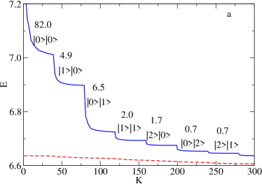
In Fig. 1a we show an example for the energy convergence of a two dimensional trion (2 electrons and a hole) coupled to 2 photon modes using the SVM with =40 basis vectors in each photon state. Initially the photon space is restricted by . First the space is optimized by adding spatial basis functions selected by SVM one by one. Then the space is added and populated by SVM and this process is repeated for each allowed photon space. The energy quickly converges in the photon spaces and the energy gain is less and less as higher photon numbers are added. The energy is not fully converged in the space so this space may need more basis functions, but in other spaces, the convergence is close to perfect and smaller spatial basis can be used. This is remedied by the refining step Sup , where the basis is improved by randomly replacing photon spaces with energetically more favorable ones. In this step, the photons can also couple photon spaces with . As the dashed line in Fig. 1a. shows, this step still significantly improves the energy.
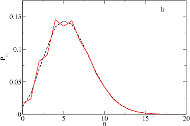
To test the accuracy of the approach we have compared the converged energies to a one-electron one-photon problem which can be solved with finite difference representation of the spatial wave function and exact diagonalization of the coupled system Flick et al. (2015, 2018b); Schafer et al. (2018). The SVM and exact diagonalization energies agree up to 5 digits for the lowest five states Sup . Fig. 1b shows photon occupation probabilities for a very strong coupling case. The SVM and the exact diagonalization results are in very good agreement, and the slight discrepancy might be due to the finite differences used in the exact diagonalization approach.
We use a harmonically confined () two-dimensional (2D) spin singlet two-electron system coupled to 2 photon modes as a second test case. The spatial part of this problem is analytically solvable and the coupled light-matter Hamiltonian can be diagonalized Huang et al. (2021). Using a.u. for the harmonic confinement, a.u. for the photon frequencies and a.u. for the coupling, the exact energy of the system is =3.65400 a.u. This choice corresponds to a diagonally polarized light and mode functions where is the length, is the volume of the cavity, and is the wave vector (). Our system is placed at the center of the cavity, and . The calculated energy 3.65401 a.u. is in perfect agreement with the analytical value and the photon space probabilities also agree Sup . This is a good and difficult test for the numerical calculation because two different couplings and many (over 80) photon states are present and photon states with very small occupation numbers contribute to the energy.
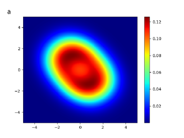
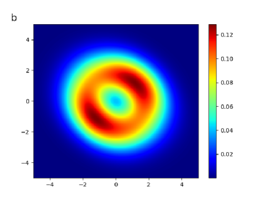
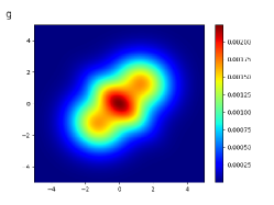
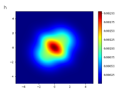
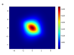
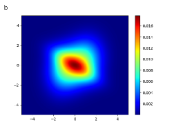
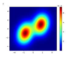
Next we study a 2D 3 electron system in harmonic confinement ( a.u.) coupled to photon mode of and . We use two dimensional examples because the visualization of the density is simpler. Without coupling to the light the electron density of these systems is spherically symmetric. The S=1/2 density has a peak in the center, while the system forms a ring-like structure due to the Pauli repulsion between the spin-polarized electrons Sup . The electron density is shown in Fig. 2 for and with a very different structure for the coupled case. The density peak in the S=1/2 case breaks up into two peaks and the S=3/2 ring also splits into two parts. This shows how strongly the light-matter coupling can change the electron density of the system.
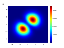

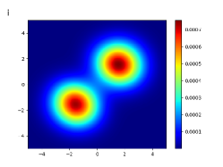
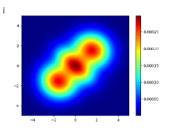
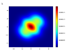

The next example is a trion, two-electron and the hole in 2D coupled to one-photon mode (parameters are in the caption of Fig. 3) and two-photon modes (Fig. 4 lists the parameters). Trions in optical microcavities in 2D semiconducting transition metal dichalcogenides have received intense experimental interest Emmanuele et al. (2020); Dhara et al. (2018); Dufferwiel et al. (2017); Sidler et al. (2017) due to the opportunities to engineer nanoscale light–matter interactions. The calculated electron densities of the trion coupled to one and two-photon modes are shown in Figs. 3 and 4. The figures show the density
| (5) |
belonging to photon state and we will also separate the contribution of electrons and hole to the density.
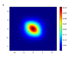
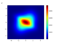
Figs. 3a and 4b show the density in the and the photon spaces. The total densities are very similar to these densities because the and photon spaces are dominant (92 and 82 percent of the wave function belongs to these states). The weights of wave functions components in photon spaces depend on the frequency and coupling, and by changing these, other photon states (or linear combinations of photon states) become major contributors to the density. The total densities are very similar to each other in the one and two-photon mode coupled cases (Figs. 3a and 4b): they are slightly squeezed along the diagonal axis. The diagonal symmetry is due to the choice of the polarization vectors.
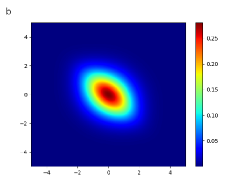
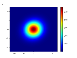
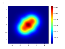
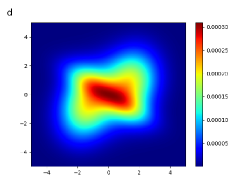
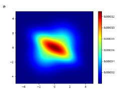
Figs. 3b and 3c show the electron and hole density of the trion in the photon space. The hole density is circularly symmetric, the electron density is elongated and the superposition of these two explains the structure seen in Fig. 3a. In the photon space the density is elongated (Fig. 3d) but now it is aligned in the direction of the diagonal. This density is a superposition of two outside electron peaks (Fig. 3e) and a hole in the middle (Fig. 3f). The photon space is similar (Fig. 3g) but now the electrons and the hole changed roles: the electron density is in the middle and the hole density has two peaks outside along the diagonal (Figs. 3h and 3i). The electron density not only has a peak in the middle but also a bond-like structure toward the hole peaks. The photon space densities (Figs. 3j, 3k, and 3l) are similar to the ones, but now the total density has three separate peaks.
In the trion coupled to the two-photon mode case (Fig. 4) we keep and the same as before and add a second photon mode with and = - . The second mode has stronger coupling because the frequency is larger. We still see gradual elongation in higher photon spaces, but the densities are quite different from the one-photon mode case. Now the photon modes elongate the density along the diagonal in certain photon spaces and perpendicular to it in other spaces. The resulted linear combinations are shown in Figs. 4b, 4c and 4d. The underlying electron and hole densities still show somewhat similar structures to the one-photon mode. For example, the total density in the photon space (Fig. 4d) is the sum of the electron density in the middle (Fig. 4e) and the two peaks of the hole (Fig 4f) outside.
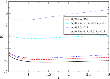
Next, we study the energy as a function of the distance between the nuclei in a 3-dimensional H2 molecule coupled to one and two-photon modes. This system was studied using one-dimensional model Hamiltonian in Refs. Hoffmann et al. (2020); Buchholz et al. (2019) to explore the role of multiphoton modes and to build better approaches to describe molecules in cavities. In this case, two protons are fixed at a distance from each other and the energy is calculated as a function of . We have studied four cases, the 4 energy curves, together with the ground state energy curve are shown in Fig. 5. The energy of the system shifts up by coupling to light, and the energy shifts higher when the coupling is larger. The effect of (not shown in the figure) is much smaller. The shift in the two-photon mode case is much larger because now two dipole self-interaction terms increase the energy. The most interesting result is that by increasing the energy minimum moves to much shorter distances. In the ground state the energy minimum is at a.u., while in the two-photon mode the equilibrium H2 bond length in the present case is (dotted line in Fig. 5) a.u.
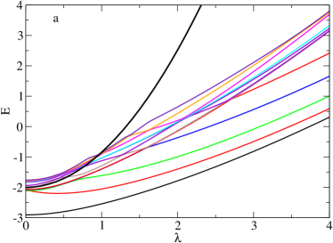
The last example is a spin singlet He atom with finite nuclear mass coupled to a single photon mode. Fig. 6a shows the lowest energy levels as a function of for a.u. Besides the bound ,, and states of the He atom, discretized continuum states (finite box approximation of the continuum states) are also included for . The thick line shows the energy of the dissociation threshold into He+ ion plus an electron. Fig. 6a shows that even some continuum states will become bound as increases. The figure also shows that certain energy levels get very close to each other and then they move away (avoided crossing). This energy level repulsion is due to the fact that changing modifies the potential shape which, in turn, drives up or down energy levels but no degeneracy is introduced and the energy levels cannot cross each other.
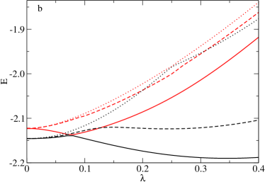
The role of is illustrated (see Fig. 6b) for the 2 and 2 energy levels. For =0.8 a.u., the 2 state moves down, approaching the 2 level at around a.u., and then it moves up while the energy of the other state decreases (and later increases as Fig 6a shows). In the case of a.u. the 2 state moves up but the closest distance between the two states (at around a.u.) is much larger than the size of the previous gap. In the a.u. case the two curves meet at a.u. These examples show that strongly influences the position of the avoided crossing points and it also affects rise of the energy curves.
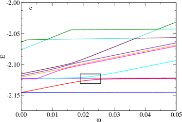
Fig. 6c shows the energy levels at even lower coupling strength. In this case we have changed keeping fixed. In this way at a.u. is 0.02 a.u. and the coupling strength is proportional to as suggested in Ref. Sidler et al. (2020) to mimic the Jaynes-Cummings model Jaynes and Cummings (1963). The box in the middle of Fig. 6c shows the position where the 2 and 2 state gets close to each other at around the a.u. transition energy and at that point the energy difference between them is 0.0055 a.u., which corresponds to a Rabi splitting of 0.1496 eV in excellent agreement with the real space grid based calculation (0.148 eV) in Ref. Sidler et al. (2020).
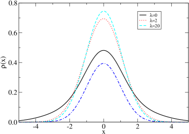
Finally, Fig. 6d shows the particle density of the He atom for different couplings. The figure shows the average density in the direction, and averaging in the or direction gives the same curve as the average in the direction. The lowest curve is the density distribution of the He nucleus and it remains the same for different values. Increasing squeezes the density toward the middle, and the system becomes more compact, but the difference between the densities for =2 a.u. and for =20 a.u. is small. This is probably because increasing couples higher photon spaces to the wave function and in these spaces the wave function components have different parity and spatial extension, so the effect of increasing is not just a simple squeezing of the density.
In summary, we have developed an approach to accurately calculate the light-matter coupled wave functions. The presented examples show that the hybrid states are very different from the original electronic states and the wave function has to be optimized in every photon space to accurately represent the system. Our approach works for charged and neutral systems, and the center of mass motion can be fixed or removed. The ECGs are limited to up to 8-10 particles due to the scaling of the explicit antisymmetrization ( is the number of identical particles in the system), but other forms of trial functions, e.g. configuration interaction type functions, might be also tested.
Acknowledgements.
This work has been supported by the National Science Foundation (NSF) under Grant No. IRES 1826917. AA, CH and MB equally contributed to this work.References
- Feist and Garcia-Vidal (2015) J. Feist and F. J. Garcia-Vidal, Phys. Rev. Lett. 114, 196402 (2015), URL https://link.aps.org/doi/10.1103/PhysRevLett.114.196402.
- Balili et al. (2007) R. Balili, V. Hartwell, D. Snoke, L. Pfeiffer, and K. West, Science 316, 1007 (2007), ISSN 0036-8075, eprint https://science.sciencemag.org/content/316/5827/1007.full.pdf, URL https://science.sciencemag.org/content/316/5827/1007.
- Schachenmayer et al. (2015) J. Schachenmayer, C. Genes, E. Tignone, and G. Pupillo, Phys. Rev. Lett. 114, 196403 (2015), URL https://link.aps.org/doi/10.1103/PhysRevLett.114.196403.
- Xiang et al. (2020) B. Xiang, R. F. Ribeiro, M. Du, L. Chen, Z. Yang, J. Wang, J. Yuen-Zhou, and W. Xiong, Science 368, 665 (2020), ISSN 0036-8075, eprint https://science.sciencemag.org/content/368/6491/665.full.pdf, URL https://science.sciencemag.org/content/368/6491/665.
- Reserbat-Plantey et al. (2021) A. Reserbat-Plantey, I. Epstein, I. Torre, A. T. Costa, P. A. D. Gonçalves, N. A. Mortensen, M. Polini, J. C. W. Song, N. M. R. Peres, and F. H. L. Koppens, ACS Photonics 8, 85 (2021), URL https://doi.org/10.1021/acsphotonics.0c01224.
- Coles et al. (2014) D. M. Coles, N. Somaschi, P. Michetti, C. Clark, P. G. Lagoudakis, P. G. Savvidis, and D. G. Lidzey, Nature Materials 13, 712 (2014), ISSN 1476-4660, URL https://doi.org/10.1038/nmat3950.
- Kasprzak et al. (2006) J. Kasprzak, M. Richard, S. Kundermann, A. Baas, P. Jeambrun, J. M. J. Keeling, F. M. Marchetti, M. H. Szymańska, R. André, J. L. Staehli, et al., Nature 443, 409 (2006), ISSN 1476-4687, URL https://doi.org/10.1038/nature05131.
- Schwartz et al. (2011) T. Schwartz, J. A. Hutchison, C. Genet, and T. W. Ebbesen, Phys. Rev. Lett. 106, 196405 (2011), URL https://link.aps.org/doi/10.1103/PhysRevLett.106.196405.
- Plumhof et al. (2014) J. D. Plumhof, T. Stöferle, L. Mai, U. Scherf, and R. F. Mahrt, Nature Materials 13, 247 (2014), ISSN 1476-4660, URL https://doi.org/10.1038/nmat3825.
- Hutchison et al. (2013) J. A. Hutchison, A. Liscio, T. Schwartz, A. Canaguier-Durand, C. Genet, V. Palermo, P. Samorì, and T. W. Ebbesen, Advanced Materials 25, 2481 (2013), eprint https://onlinelibrary.wiley.com/doi/pdf/10.1002/adma.201203682, URL https://onlinelibrary.wiley.com/doi/abs/10.1002/adma.201203682.
- Wang et al. (2021a) K. Wang, M. Seidel, K. Nagarajan, T. Chervy, C. Genet, and T. Ebbesen, Nature Communications 12, 1486 (2021a), ISSN 2041-1723, URL https://doi.org/10.1038/s41467-021-21739-7.
- Basov et al. (2021) D. N. Basov, A. Asenjo-Garcia, P. J. Schuck, X. Zhu, and A. Rubio, Nanophotonics 10, 549 (2021), URL https://doi.org/10.1515/nanoph-2020-0449.
- Mazza and Georges (2019) G. Mazza and A. Georges, Phys. Rev. Lett. 122, 017401 (2019), URL https://link.aps.org/doi/10.1103/PhysRevLett.122.017401.
- Di Stefano et al. (2019) O. Di Stefano, A. Settineri, V. Macrì, L. Garziano, R. Stassi, S. Savasta, and F. Nori, Nature Physics 15, 803 (2019), ISSN 1745-2481, URL https://doi.org/10.1038/s41567-019-0534-4.
- Galego et al. (2015) J. Galego, F. J. Garcia-Vidal, and J. Feist, Phys. Rev. X 5, 041022 (2015), URL https://link.aps.org/doi/10.1103/PhysRevX.5.041022.
- Herrera and Spano (2016) F. Herrera and F. C. Spano, Phys. Rev. Lett. 116, 238301 (2016), URL https://link.aps.org/doi/10.1103/PhysRevLett.116.238301.
- Galego et al. (2016) J. Galego, F. J. Garcia-Vidal, and J. Feist, Nature Communications 7, 13841 (2016), ISSN 2041-1723, URL https://doi.org/10.1038/ncomms13841.
- Shalabney et al. (2015) A. Shalabney, J. George, J. Hutchison, G. Pupillo, C. Genet, and T. W. Ebbesen, Nature Communications 6, 5981 (2015), ISSN 2041-1723, URL https://doi.org/10.1038/ncomms6981.
- Buchholz et al. (2019) F. Buchholz, I. Theophilou, S. E. B. Nielsen, M. Ruggenthaler, and A. Rubio, ACS Photonics 6, 2694 (2019).
- Schäfer et al. (2019) C. Schäfer, M. Ruggenthaler, H. Appel, and A. Rubio, Proceedings of the National Academy of Sciences 116, 4883 (2019), ISSN 0027-8424, eprint https://www.pnas.org/content/116/11/4883.full.pdf, URL https://www.pnas.org/content/116/11/4883.
- Ruggenthaler et al. (2018) M. Ruggenthaler, N. Tancogne-Dejean, J. Flick, H. Appel, and A. Rubio, Nature Reviews Chemistry 2, 0118 (2018), ISSN 2397-3358, URL https://doi.org/10.1038/s41570-018-0118.
- Flick et al. (2015) J. Flick, M. Ruggenthaler, H. Appel, and A. Rubio, Proceedings of the National Academy of Sciences 112, 15285 (2015), ISSN 0027-8424, eprint https://www.pnas.org/content/112/50/15285.full.pdf, URL https://www.pnas.org/content/112/50/15285.
- Flick et al. (2017) J. Flick, M. Ruggenthaler, H. Appel, and A. Rubio, Proceedings of the National Academy of Sciences 114, 3026 (2017), ISSN 0027-8424, eprint https://www.pnas.org/content/114/12/3026.full.pdf, URL https://www.pnas.org/content/114/12/3026.
- Lacombe et al. (2019) L. Lacombe, N. M. Hoffmann, and N. T. Maitra, Phys. Rev. Lett. 123, 083201 (2019), URL https://link.aps.org/doi/10.1103/PhysRevLett.123.083201.
- Mandal et al. (2020a) A. Mandal, S. Montillo Vega, and P. Huo, The Journal of Physical Chemistry Letters 11, 9215 (2020a), pMID: 32991814.
- Flick et al. (2019) J. Flick, D. M. Welakuh, M. Ruggenthaler, H. Appel, and A. Rubio, ACS Photonics 6, 2757 (2019).
- Latini et al. (2019) S. Latini, E. Ronca, U. De Giovannini, H. Hübener, and A. Rubio, Nano Letters 19, 3473 (2019), pMID: 31046291.
- Flick et al. (2018a) J. Flick, N. Rivera, and P. Narang, Nanophotonics 7, 1479 (2018a), URL https://doi.org/10.1515/nanoph-2018-0067.
- Flick and Narang (2018) J. Flick and P. Narang, Phys. Rev. Lett. 121, 113002 (2018), URL https://link.aps.org/doi/10.1103/PhysRevLett.121.113002.
- Garcia-Vidal et al. (2021) F. J. Garcia-Vidal, C. Ciuti, and T. W. Ebbesen, Science 373 (2021), ISSN 0036-8075, eprint https://science.sciencemag.org/content/373/6551/eabd0336.full.pdf, URL https://science.sciencemag.org/content/373/6551/eabd0336.
- Thomas et al. (2019) A. Thomas, L. Lethuillier-Karl, K. Nagarajan, R. M. A. Vergauwe, J. George, T. Chervy, A. Shalabney, E. Devaux, C. Genet, J. Moran, et al., Science 363, 615 (2019), ISSN 0036-8075, eprint https://science.sciencemag.org/content/363/6427/615.full.pdf, URL https://science.sciencemag.org/content/363/6427/615.
- Mordovina et al. (2020) U. Mordovina, C. Bungey, H. Appel, P. J. Knowles, A. Rubio, and F. R. Manby, Phys. Rev. Research 2, 023262 (2020), URL https://link.aps.org/doi/10.1103/PhysRevResearch.2.023262.
- Wang et al. (2021b) D. S. Wang, T. Neuman, J. Flick, and P. Narang, The Journal of Chemical Physics 154, 104109 (2021b).
- DePrince (2021) A. E. DePrince, The Journal of Chemical Physics 154, 094112 (2021), URL https://doi.org/10.1063/5.0038748.
- Haugland et al. (2021) T. S. Haugland, C. Schäfer, E. Ronca, A. Rubio, and H. Koch, The Journal of Chemical Physics 154, 094113 (2021), URL https://doi.org/10.1063/5.0039256.
- Hoffmann et al. (2020) N. M. Hoffmann, L. Lacombe, A. Rubio, and N. T. Maitra, The Journal of Chemical Physics 153, 104103 (2020).
- Flick and Narang (2020) J. Flick and P. Narang, The Journal of Chemical Physics 153, 094116 (2020), URL https://doi.org/10.1063/5.0021033.
- Mandal et al. (2020b) A. Mandal, T. D. Krauss, and P. Huo, The Journal of Physical Chemistry B 124, 6321 (2020b), pMID: 32589846.
- Galego et al. (2017) J. Galego, F. J. Garcia-Vidal, and J. Feist, Phys. Rev. Lett. 119, 136001 (2017), URL https://link.aps.org/doi/10.1103/PhysRevLett.119.136001.
- Flick et al. (2018b) J. Flick, C. Schäfer, M. Ruggenthaler, H. Appel, and A. Rubio, ACS Photonics 5, 992 (2018b).
- Schafer et al. (2018) C. Schafer, M. Ruggenthaler, and A. Rubio, Phys. Rev. A 98, 043801 (2018), URL https://link.aps.org/doi/10.1103/PhysRevA.98.043801.
- Sidler et al. (2020) D. Sidler, M. Ruggenthaler, H. Appel, and A. Rubio, The Journal of Physical Chemistry Letters 11, 7525 (2020), pMID: 32805122, URL https://doi.org/10.1021/acs.jpclett.0c01556.
- Theophilou et al. (2020) I. Theophilou, M. Penz, M. Ruggenthaler, and A. Rubio, Journal of Chemical Theory and Computation 16, 6236 (2020), pMID: 32816479, URL https://doi.org/10.1021/acs.jctc.0c00618.
- Sidler et al. (2021) D. Sidler, C. Schäfer, M. Ruggenthaler, and A. Rubio, The Journal of Physical Chemistry Letters 12, 508 (2021), pMID: 33373238, URL https://doi.org/10.1021/acs.jpclett.0c03436.
- Buchholz et al. (2020) F. Buchholz, I. Theophilou, K. J. H. Giesbertz, M. Ruggenthaler, and A. Rubio, Journal of Chemical Theory and Computation 16, 5601 (2020), pMID: 32692551, URL https://doi.org/10.1021/acs.jctc.0c00469.
- Tokatly (2018) I. V. Tokatly, Phys. Rev. B 98, 235123 (2018), URL https://link.aps.org/doi/10.1103/PhysRevB.98.235123.
- Rivera et al. (2019) N. Rivera, J. Flick, and P. Narang, Phys. Rev. Lett. 122, 193603 (2019), URL https://link.aps.org/doi/10.1103/PhysRevLett.122.193603.
- Szidarovszky et al. (2020) T. Szidarovszky, G. J. Halász, and Á. Vibók, New Journal of Physics 22, 053001 (2020), URL https://doi.org/10.1088/1367-2630/ab8264.
- Cederbaum (2021) L. S. Cederbaum, The Journal of Physical Chemistry Letters 12, 6056 (2021), pMID: 34165990, URL https://doi.org/10.1021/acs.jpclett.1c01570.
- Thomas et al. (2016) A. Thomas, J. George, A. Shalabney, M. Dryzhakov, S. J. Varma, J. Moran, T. Chervy, X. Zhong, E. Devaux, C. Genet, et al., Angewandte Chemie International Edition 55, 11462 (2016), eprint https://onlinelibrary.wiley.com/doi/pdf/10.1002/anie.201605504, URL https://onlinelibrary.wiley.com/doi/abs/10.1002/anie.201605504.
- Puchalski et al. (2019) M. Puchalski, J. Komasa, P. Czachorowski, and K. Pachucki, Phys. Rev. Lett. 122, 103003 (2019), URL https://link.aps.org/doi/10.1103/PhysRevLett.122.103003.
- Hölsch et al. (2019) N. Hölsch, M. Beyer, E. J. Salumbides, K. S. E. Eikema, W. Ubachs, C. Jungen, and F. Merkt, Phys. Rev. Lett. 122, 103002 (2019), URL https://link.aps.org/doi/10.1103/PhysRevLett.122.103002.
- Kohn and Sham (1965) W. Kohn and L. J. Sham, Phys. Rev. 140, A1133 (1965), URL https://link.aps.org/doi/10.1103/PhysRev.140.A1133.
- Mitroy et al. (2013) J. Mitroy, S. Bubin, W. Horiuchi, Y. Suzuki, L. Adamowicz, W. Cencek, K. Szalewicz, J. Komasa, D. Blume, and K. Varga, Rev. Mod. Phys. 85, 693 (2013), URL https://link.aps.org/doi/10.1103/RevModPhys.85.693.
- Suzuki et al. (1998) Y. Suzuki, M. Suzuki, and K. Varga, Stochastic variational approach to quantum-mechanical few-body problems, vol. 54 (Springer Science & Business Media, 1998).
- Cioslowski and Strasburger (2017) J. Cioslowski and K. Strasburger, The Journal of Chemical Physics 146, 044308 (2017), URL https://doi.org/10.1063/1.4974273.
- Zaklama et al. (2019) T. Zaklama, D. Zhang, K. Rowan, L. Schatzki, Y. Suzuki, and K. Varga, Few-Body Systems 61, 6 (2019), ISSN 1432-5411, URL https://doi.org/10.1007/s00601-019-1539-3.
- Zhang et al. (2015) D. K. Zhang, D. W. Kidd, and K. Varga, Nano Letters 15, 7002 (2015), ISSN 1530-6984, URL https://doi.org/10.1021/acs.nanolett.5b03009.
- Kidd et al. (2016) D. W. Kidd, D. K. Zhang, and K. Varga, Phys. Rev. B 93, 125423 (2016), URL https://link.aps.org/doi/10.1103/PhysRevB.93.125423.
- Riva et al. (2000) C. Riva, F. M. Peeters, and K. Varga, Phys. Rev. B 61, 13873 (2000), URL https://link.aps.org/doi/10.1103/PhysRevB.61.13873.
- Varga (1999) K. Varga, Phys. Rev. Lett. 83, 5471 (1999), URL https://link.aps.org/doi/10.1103/PhysRevLett.83.5471.
- Usukura et al. (1999) J. Usukura, Y. Suzuki, and K. Varga, Phys. Rev. B 59, 5652 (1999), URL https://link.aps.org/doi/10.1103/PhysRevB.59.5652.
- Varga et al. (2001) K. Varga, P. Navratil, J. Usukura, and Y. Suzuki, Phys. Rev. B 63, 205308 (2001), URL https://link.aps.org/doi/10.1103/PhysRevB.63.205308.
- Rokaj et al. (2018) V. Rokaj, D. M. Welakuh, M. Ruggenthaler, and A. Rubio, Journal of Physics B: Atomic, Molecular and Optical Physics 51, 034005 (2018), URL https://doi.org/10.1088/1361-6455/aa9c99.
- Ruggenthaler et al. (2014) M. Ruggenthaler, J. Flick, C. Pellegrini, H. Appel, I. V. Tokatly, and A. Rubio, Phys. Rev. A 90, 012508 (2014), URL https://link.aps.org/doi/10.1103/PhysRevA.90.012508.
- (66) (????), see Supplemental Material.
- Kukulin and Krasnopol’sky (1977) V. I. Kukulin and V. M. Krasnopol’sky, J. Phys. G 3, 795 (1977).
- Huang et al. (2021) C. Huang, A. Ahrens, M. Beutel, and K. Varga, Two electrons in harmonic confinement coupled to light in a cavity (2021), eprint 2108.01702.
- Emmanuele et al. (2020) R. P. A. Emmanuele, M. Sich, O. Kyriienko, V. Shahnazaryan, F. Withers, A. Catanzaro, P. M. Walker, F. A. Benimetskiy, M. S. Skolnick, A. I. Tartakovskii, et al., Nature Communications 11, 3589 (2020), ISSN 2041-1723, URL https://doi.org/10.1038/s41467-020-17340-z.
- Dhara et al. (2018) S. Dhara, C. Chakraborty, K. M. Goodfellow, L. Qiu, T. A. O’Loughlin, G. W. Wicks, S. Bhattacharjee, and A. N. Vamivakas, Nature Physics 14, 130 (2018), ISSN 1745-2481, URL https://doi.org/10.1038/nphys4303.
- Dufferwiel et al. (2017) S. Dufferwiel, T. P. Lyons, D. D. Solnyshkov, A. A. P. Trichet, F. Withers, S. Schwarz, G. Malpuech, J. M. Smith, K. S. Novoselov, M. S. Skolnick, et al., Nature Photonics 11, 497 (2017), ISSN 1749-4893, URL https://doi.org/10.1038/nphoton.2017.125.
- Sidler et al. (2017) M. Sidler, P. Back, O. Cotlet, A. Srivastava, T. Fink, M. Kroner, E. Demler, and A. Imamoglu, Nature Physics 13, 255 (2017), ISSN 1745-2481, URL https://doi.org/10.1038/nphys3949.
- Jaynes and Cummings (1963) E. Jaynes and F. Cummings, Proceedings of the IEEE 51, 89 (1963).