Unified generation and fast emission of arbitrary single-photon multimode $W$ states

Abstract

We propose a unified and deterministic scheme to generate arbitrary single-photon multimode $W$ states in circuit QED. A three-level system (qutrit) is driven by a pump-laser pulse and coupled to $N$ spatially separated resonators. The coupling strength for each spatial mode $g_{i}$ totally decide the generated single-photon N-mode $W$ state $|W_{N}\rangle=\frac{1}{A}\sum_{i=1}^{N}g_{i}|0_{1}0_{2}\cdots 1_{i}0_{i+1}\cdots 0_{N}\rangle$, so arbitrary $|W_{N}\rangle$ can be generated just by tuning $g_{i}$. We could not only generate $W$ states inside resonators but also release them into transmission lines on demand. The time and fidelity for generating (or emitting) $|W_{N}\rangle$ can both be the same for arbitrary $N$. Remarkably, $|W_{N}\rangle$ can be emitted with probability reaching $98.9\%$ in $20-50$ ns depending on parameters, comparable to the recently reported fastest two-qubit gate ($30-45$ ns). Finally, the time evolution process is convenient to control since only the pump pulse is time-dependent.

INTRODUCTION

Entanglement is essential to quantum information, which is widely applied in quantum dense coding 2881 (1992) , quantum teleportation 1895 (1993) , quantum cryptography 661 (1991) , and quantum computing 325 (1997) . It was first proposed by Einstein, Podolsky, and Rosen (EPR) to challenge the completeness of quantum mechanics 777 (1935) . There are two inequivalent categories of tripartite entanglement state, the Greenberger-Horne-Zeilinger (GHZ) state George Mason University press ; yangcp1 ; yangcp2 ; npj and the $W$ state 062314 (2000) ; oz , which could be used to prove Bell’s theorem without inequalities 032108 (2002) . Notably, the $W$ state is more robust than the GHZ state since if one particle is traced out, it retains multiparticle entanglement 032108 (2002) . Extending it to the multipartite case, the general form of a $W$ state is prx 2013 ; asaa

$$|W_{N}\rangle=\dfrac{1}{A}\sum_{i=1}^{N}A_{i}|0_{1}0_{2}\cdots 1_{i}0_{i+1}\cdots 0_{N}\rangle$$ (1)

where $A=\sqrt{\sum A_{i}^{2}}$. $|1\rangle$ and $|0\rangle$ represent two orthogonal states encoded in frequencies 013845 (2016) ; 070508 (2019) , polarizations 10151 (2019) ; 077901 (2004) ; 044302 (2002) , or spatial modes 012308 (2016) ; 022337 (2020) ; jie of photons, or qubit energy state67 (2018) ; 042102 (2002) ; 014302 (2006) .

Various schemes for preparing $W$ states have been proposed, via spontaneous four-wave mixing 013845 (2016) ; 070508 (2019) , polarizing beam splitter (PBS)10151 (2019) ; 077901 (2004) ; 044302 (2002) , cavity QED 042102 (2002) ; 014302 (2006) ; 054302 (2002) , circuit QED jie ; 812(2015) ; yanxia1 ; yanxia2 ; prl 2020 ; circuit , cold neutral atoms stoj , spin system spin and so on. However, a unified scheme to generate arbitrary $W$ states with high fidelity, speed, and feasibility is needed. First, $W$ states are useful from lower-order to higher-order, since the later establishes entanglement between a large number of channels, making them favourable for realization of quantum information process. E.g., Gottesman et al. has shown this state is beneficial in longer baseline telescopes 070503 (2012) . However, the preparation of higher-order W-states often involves complex bulk-optical set-ups pra 2013 ; science 2009 ; nature 2010 , and the scheme is complex. Second, the coefficient of each basis needs to be easily tunable, because sometimes we require not only the maximum entangled $W$ state where all $A_{i}$’s are equal keli , but also some other types. E. g., the prototype $W$ state $|W_{3}\rangle={1}/{\sqrt{3}}(|100\rangle+|010\rangle+|001\rangle)$ is not suitable for quantum teleportation 267 (2003) , while another one $|W^{\prime}_{3}\rangle={1}/{2}(|100\rangle+|010\rangle+\sqrt{2}|001\rangle)$ proposed by Agrawal and Pati is perfect for teleportation and superdense coding 062320 (2006) ; 10871 (2007) . It has been demonstrated that different $W$ states of identical qubits could be transformed by entanglement concentration 042302 (2012) ; 71 (2013) , but the process is complex. Third, states must be generated with high speed and fidelity to accelerate the operation and avoid decoherence in practical quantum information processing. Besides, the scheme should be easy to realize with high experimental feasibility.

In this paper, we present a unified deterministic scheme to generate arbitrary single-photon multimode $W$ states $|W_{N}\rangle$, satisfying the aforementioned requirements. We have a qutrit yangcp3 (e.g., a $\Lambda$ type superconducting quantum interference device (SQUID)024303(2015) ; 064303(2006) , transmon transmon1 ; transmon2 ; transmon3 or an Xmon xmon ) driven by pump-laser pulses and coupled to $N$ spatially separated resonators, to obtain $|W_{N}\rangle$ Eq. (1) with $A_{i}$ equaling the coupling strength between the $i$-th resonator mode and the qutrit, $g_{i}$. Hence we can generate arbitrary $W$ state just by adjusting $g_{i}$. We can not only create $|W_{N}\rangle$ inside resonators through adiabatic evolution along a dark state, but also emit it into transmission lines through dissipation. The emission probability reaches $98.9\%$ in $20-50$ ns, comparable to the fastest two-qubit gate ($30-45$ ns) recently reported (ns, ). The generation (or emission) time and fidelity (or probability) can both be the same for arbitrary mode numbers. Besides, we only need to tune the pump pulse during the whole time evolution process, which is easier to control than the qutrit and resonators.

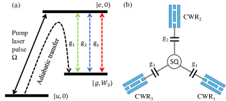
FIG. 1: Scheme of generating the three-mode single-photon $W$ state $|W_{3}\rangle$ inside resonators through adiabatic passage. a Relevant energy levels and transitions. The qutrit states are labeled by $|u\rangle$, $|e\rangle$, and $|g\rangle$. $|0\rangle$ and $|1\rangle$ denote the photon number states in the resonator. b Setup: A superconducting qutrit (SQ) is capacitively coupled to three coplanar waveguide resonators (CWRs) with coupling strength $g_{1}$, $g_{2}$, $g_{3}$ and a pump laser pulse with rabi frequency $\Omega$.

RESULTS

Generating the single-photon three-mode $W$ state inside resonators

Although we aim to generate arbitrary $N$-mode $W$ state, we start with the prototype three-mode case, with our our scheme depicted in Fig. 1. The qutrit has a $\Lambda$-type configuration formed by two lowest levels $|u\rangle$ and $|g\rangle$ and an excited level $|e\rangle$. The resonator state is denoted by $|n\rangle$, where $n$ is the number of photons. Three resonator modes only couple $|e,n\rangle$ and $|g,n+1\rangle$ with coupling strengths $g_{1}$, $g_{2}$, and $g_{3}$ respectively, whose frequencies are identical and far off resonance from the $|e,n\rangle$ to $|u,n\rangle$ transition. Similarly, a pump laser pulse with Rabi frequency $\Omega$ only couples $|e,n\rangle$ to $|u,n\rangle$ for the same reason, as shown in Fig 1. The system is initially in $|u,0\rangle$ and evolved into $|g,W_{3}\rangle$ through an adiabatic passage along a dark state.

In the one-photon manifold $\{|u,000\rangle,|e,000\rangle,|g,100\rangle,$
$|g,010\rangle,|g,001\rangle\}$ under rotating wave approximation, the Hamiltonian reads $(\hbar=1)$ 373 (1999) ; 023601 (2005) :

$$H = \sum_{i=u,e}E_{i}|i,000\rangle\langle i,000|+(E_{g}+\omega)(|g,100\rangle\langle g,100|$$ (2)

$$+|g,010\rangle\langle g,010|+|g,001\rangle\langle g,001|)$$

$$+[\dfrac{1}{2}\Omega e^{-i\omega_{P}t}|e,000\rangle\langle u,000|+g_{1}|e,000\rangle\langle g,100|$$

$$+g_{2}|e,000\rangle\langle g,010|+g_{3}|e,000\rangle\langle g,001|+H.c.]$$

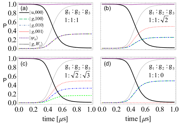
FIG. 2: Adiabatic transfer from $|u,000\rangle$ to $|g,W_{3}\rangle$ obtained by numerical simulation. Population of states $|u,000\rangle$, $|g,100\rangle$, $|g,010\rangle$, $|g,001\rangle$, dark state $|\Psi_{0}\rangle$ and final state $|g,W_{3}\rangle$, as a function of time for $\Delta_{1}=\Delta_{2}=0$ MHz, $\Omega=\Omega_{0}exp[-(t-\tau)^{2}/T_{0}^{2}]$, with $\Omega_{0}=2\pi\times 700$ MHz, $T_{0}=0.36\mu$ s, and $\tau=1\mu$ s. The couplings in figures a,b,c,d are $2g_{1}/2\pi=45$ MHz, $38$ MHz, $31$ MHz, $54$ MHz, respectively.

where $E_{i}$ represents the eigenvalue of the $i$-th energy level, $\omega$ is the frequency of each resonator. $\omega_{P}$ is the frequency of the pump pulse.

In the interaction picture (see “Methods” section), there are three degenerate dark states $\{2g_{1}|u,000\rangle-\Omega|g,100\rangle,~{}2g_{2}|u,000\rangle-\Omega|g,010\rangle,~{}2g_{3}|u,000\rangle-\Omega|g,001\rangle\}$ with constant eigenenergy $E=0$ under two-photon resonance condition, where the detunings of the pump-laser, $\Delta_{1}$, and the resonators, $\Delta_{2}$, from the respective qutrit transitions are equal 373 (1999) ; determine . According to the Schrödinger equation of the system with initial state $|u,000\rangle$, we find the dark state in this specific case to be (see “Methods” section)

$$|\Psi_{0}\rangle = \frac{1}{{\sqrt{4A^{2}+\Omega^{2}}}}[2A|u,000\rangle-\Omega|g,W_{3}\rangle],$$ (3)

where $A=\sqrt{\sum_{i=1}^{3}g_{i}^{2}}$, $|W_{3}\rangle=\frac{1}{A}(g_{1}|100\rangle+g_{2}|010\rangle+g_{3}|001\rangle)$.

Since $g_{i}$ is adjustable, the dark state $|\Psi_{0}\rangle$ can be used to generate arbitrary single-photon three-mode $W$ states inside resonators. First we set $g_{1}:g_{2}:g_{3}$ on demand, and then turn on the pump pulse which rises slowly enough to ensure the adiabatic transfer from $|u,000\rangle$ to $|g\rangle\otimes|W_{3}\rangle$ when $\Omega\gg g_{i}$. Choosing the pump pulse $\Omega=\Omega_{0}exp[-(t-\tau)^{2}/T_{0}^{2}]$, with $\Omega_{0}=2\pi\times 700$ MHz Pechal , $T_{0}=0.36\mu s$, and $\tau=1\mu s$, we simulate the time evolution of the system by solving the Schrödinger equation numerically. As can be seen in Fig. 2, the adiabatic fidelity 145501 (2014) ; 2433 (1995) ; Cambridge UK (2000) $|\langle\psi(t)|\Psi_{0}\rangle|^{2}$ is close to $1$ at all time and the fidelity $F(t)=|\langle\psi(t)|g,W_{3}\rangle|^{2}$ increases as the pump pulse rises and finally approaches unity when $\Omega\gg g_{i}$. Consequently, our proposal is testified by numerical results. Ideally, $F(t)$ finally reaches $\Omega_{0}^{2}/(4A^{2}+\Omega_{0}^{2})$ at $t=\tau$. Since the highest $\Omega_{0}/2\pi$ we find in experiments $\approx 1$ GHz Pechal , $A/2\pi$ can be some tens of MHz to ensure a high fidelity at the end of the adiabatic evolution. Meanwhile, the gap limiting the evolution speed is $\frac{1}{2}(\Delta_{1}-\sqrt{4A^{2}+\Omega^{2}+\Delta_{1}^{2}})$. Therefore $\tau\ll A^{-1}$ 373 (1999) according to the adiabatic theorem sa , which is limited to some hundreds of ns. Here $\tau=1\mu s$ and $F(\tau)\approx 99\%$. Selecting specific couplings, we can generate a prototype $W$ state $1/\sqrt{3}(|100\rangle+|010\rangle+|001\rangle)$, shown in Fig. 2a, a perfect $W$ state $1/2(|100\rangle+|010\rangle+\sqrt{2}|001\rangle)$ in Fig. 2b, a common one $1/\sqrt{6}(|100\rangle+1/\sqrt{2}|010\rangle+\sqrt{3}|001\rangle)$ in Fig. 2c and a Bell state $1/\sqrt{2}(|10\rangle+|01\rangle)$ in Fig. 2d.

Emission of the single-photon three-mode $W$ states

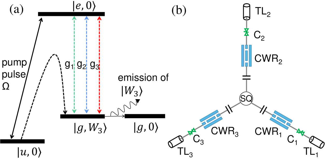
FIG. 3: The scheme to emit the single-photon three-mode $W$ state $|W_{3}\rangle$. (a) Relevant energy levels and transitions. (b) Setup: We add a variable coupler to control the dissipation rate of each CWR into the corresponding transmission line (TL) yin .

Our scheme to emit the single photon $W$ state is shown in Fig. 3. Each CWR is coupled to a transmission line (TL) through a variable coupler C, so that its dissipation rate $\kappa$ into the TL is tunable yin . We are able to generate a single photon $W$ state inside CWRs when C is turned off, as discussed above. If we turn on each C with the same $\kappa$, then the $W$ state is released into the TLs, overcoming its disadvantage of uneasy to be detected 054302 (2002) . First, we give an intuitive explanation. Any initial superposition state of the form

$$g_{1}|g,100\rangle+g_{2}|g,010\rangle+g_{3}|g,001\rangle$$ (4)

will be finally transformed to

$$|g,000\rangle\otimes(g_{1}|100\rangle_{out}+g_{2}|010\rangle_{out}+g_{3}|001\rangle_{out})$$ (5)

through leakage resonators with the same dissipation rate, where $|100\rangle_{out},|010\rangle_{out},|010\rangle_{out}$ denote there is one photon in the output channel of the first, second and third resonators respectively, considering $a_{iout}(t)=\sqrt{\kappa_{i}}a_{i}(t),~{}~{}~{}i=1,2,3$ Pechal ; input in the Heisenberg picture. A more rigorous analysis is shown in “Methods” section.

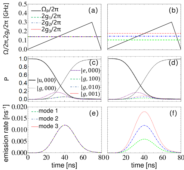
FIG. 4: Simulated emission of the $W$ state using the Lindblad master equation (11). $|W_{3}\rangle=\frac{1}{\sqrt{3}}(|100\rangle+|010\rangle+|001\rangle)$ in the left panel and $\frac{1}{\sqrt{6}}(|100\rangle+\sqrt{2}|010\rangle+\sqrt{3}|001\rangle)$ in the right panel, for $\Delta_{1}=\Delta_{2}=2\pi\times 20$ MHz, $\gamma=\gamma_{\phi}=2\pi\times 0.04$ MHz, $\kappa_{i}=\kappa=0.2$ GHz. (a) and (b) Pump pulses and coupling strength between qutrit and each resonator. c, d Population of states $|u,000\rangle$, $|g,100\rangle$, $|g,010\rangle$, $|g,001\rangle$, $|g,000\rangle$ inside resonators. e, f Emission rate of each mode into the transmission line.

In realistic imperfect experimental setups, $\kappa_{i}$ includes a intrinsic part and another one caused by the coupler $C$. The former is neglected here because it can be chosen as $1/1000$ of the later in experiment yin . The qutrit excited state $|e\rangle$ possesses a lifetime $(2\gamma)^{-1}$, where we have assumed its decay rates to $|u\rangle$ and $|g\rangle$ are equal, and a dephasing time $(\gamma_{\phi})^{-1}$. Choosing the pump pulse $\Omega$ and coupling $g_{i}$ as shown in Fig. 4a, b, the population transfer under dissipation are obtained by solving the Lindblad master equation (see “Methods” section) numerically, and shown in Fig. 4c, d. The single-photon $W$ state is created at the rising edge of the pump pulse and emitted through the leakage resonators, so the system will end up with a product state $|g,000\rangle$. Choosing $\kappa_{i}=\kappa=2\pi\times 0.2$ GHz yin , $\gamma=\gamma_{\phi}=2\pi\times 0.04$ MHz blas , $\Omega_{max}/2\pi=0.3$ GHz prl 2009 , which are within the reach of experiment, the $W$ states can be emitted in $80$ ns with probabilities reaching $99.1\%$, as shown in Fig. 4e, f. The emission rate and probability of the $i$-th resonator are proportional to $g_{i}^{2}$ for $\kappa_{i}=\kappa$, which means that the output single-photon state could still possesses the structure of $g_{1}|100\rangle+g_{2}|010\rangle+g_{3}|001\rangle$, an easily tunable $W$ state. This process is fast and the population of $|e,000\rangle$ is not always zero, as can be seen in Fig. 4c, d. However, this will not hinder the emission of $|W_{3}\rangle$ since the damping rate of $|e\rangle$ is very small. Its population will be transferred to $|g,1\rangle$, and then the single photon will still be emitted through resonator dissipation.

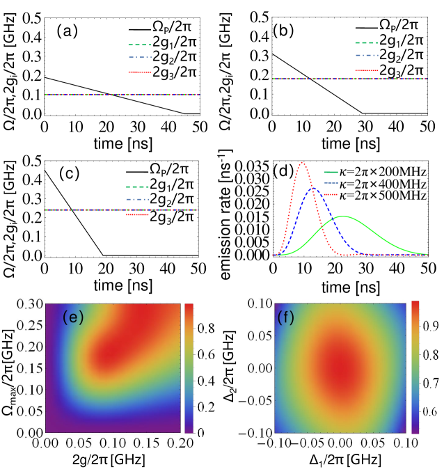
FIG. 5: Simulated fast emission of the $W$ state using certain combination of parameters. a, b, c $g_{i}$ and $\Omega$ used for $\kappa/2\pi=200$ MHz, $400$ MHz, $500$ MHz in numerical simulation, respectively. d The photon wave packets of each mode, which are overlapped since the emission rates are equal. e Emission probabilities in $50$ ns against $g$ and $\Omega_{max}$, for $\kappa/2\pi=200$ MHz, $\gamma=\gamma_{\phi}=2\pi\times 0.04$ MHz, and $\Delta_{1}=\Delta_{2}=0$. f Emission probabilities in $50$ ns against $\Delta_{1}$ and $\Delta_{2}$, for $\kappa/2\pi=200$ MHz, $\Omega$ and $g$ chosen as a, and $\gamma=\gamma_{\phi}=2\pi\times 0.04$ MHz.

The emission rate and probability depend on $g_{i}$, $\kappa$, $\gamma$, $\gamma_{\phi}$, $\Delta_{1}$, $\Delta_{2}$ and $\Omega$, and we shall explorer a combination of parameters available for fast rate and high probability. For simplicity, we consider $g=g_{1}=g_{2}=g_{3}$, so that the photon emission rate for three resonators are the same and their wave packets are overlapped. The maximum $\kappa$ we found in experiment is $2\pi\times 200$ MHz yin , but in principle, it could be larger in the bad-cavity limit blas ; law ; nc . So we consider $\kappa/2\pi=200$ MHz, $400$ MHz, $500$ MHz, and choose different combinations of $\Omega$ and $g$ for the fast emission of the $W$ state, which are shown in Fig. 5a, b, c respectively. The corresponding emission probabilities of the prototype $W$ state reach $98.9\%$ in $50$ ns, $99.5\%$ in $30$ ns and $98.9\%$ in $20$ ns, respectively, as shown in Fig. 5d, comparable to the recently reported fastest two-qubit gate ($30-45$ ns) ns . Here $\gamma=\gamma_{\phi}$ is fixed at $2\pi\times 0.04$ MHz blas , and $\Delta_{1}=\Delta_{2}=0$. These parameters are chosen based on analyses and numerical experiments. First, as can be seen, a combination of larger $\kappa$, $g$ and $\Omega$ will make the photon wave packet sharper and shifted towards earlier time. The system is initially in $|u,0\rangle$, so a large $\Omega$ will transfer the population to $|e,0\rangle$ quickly. Meanwhile, a proper combination of $g$ and $\kappa$ will quickly transfer the population of $|e,0\rangle$ to $|g,1\rangle$ and release the photon. $\Omega$ is supposed to decrease as the population of $|u\rangle$ decreases to avoid too much repumping from $|e\rangle$ to $|u\rangle$ and enhance the proportion of $|e,0\rangle\rightarrow|g,1\rangle$ transition. Therefore, we choose a linear decreasing shape of the drive pulse, which gives the fastest emission rate in our numerical tests. We limit the total evolution time $T=50$ ns, and $\Omega(t)=\Omega_{max}(1-t/t_{f})$. Taking $\kappa/2\pi=200$ MHz for example, we choose $t_{f}=45$ ns, and search for the best combination of $g_{i}$ and $\Omega_{max}$ to give the maximum emission probability numerically, as shown in Fig. 5e. The best choice ($2g/2\pi=0.1$ GHz, $\Omega_{max}/2\pi=0.19$ GHz) is depicted in Fig. 5 a. Second, damping $\gamma$ and dephasing $\gamma_{\phi}$ will reduce the emission probability, so we choose very small $\gamma$ and $\gamma_{\phi}$ available for superconducting qubits blas . Last, for the case shown in Fig. 5a with $\kappa/2\pi=200$ MHz, we change parameters $\Delta_{1}$ and $\Delta_{2}$ to find the maximum emission probability reach at the resonance condition $\Delta_{1}=\Delta_{2}=0$, as shown in Fig. 5f.

Generation and emission of arbitrary single-photon multimode $W$ states with the same fidelity and time

Here we extend our scheme to generate and emit arbitrary single-photon multimode $W$ states $|W_{N}\rangle=\frac{1}{A}\sum A_{i}|0_{1}0_{2}\cdots 1_{i}0_{i+1}\cdots 0_{N}\rangle$. The system is in principle the same as Fig. 3, just with resonator number added to $N$.

The Hamiltonian of this system becomes

$$H = \sum_{j=u,e,g}E_{j}|j,00...0\rangle\langle j,00...0|$$

$$+(E_{g}+\omega)(\sum_{i=1}^{N}|g,0_{1}0_{2}\cdots 1_{i}0_{i+1}\cdots 0_{N}\rangle$$

$$\otimes\langle g,0_{1}0_{2}\cdots 1_{i}0_{i+1}\cdots 0_{N}|)$$

$$+[\dfrac{1}{2}\Omega_{T}e^{-i\omega_{P}t}|e,00...0\rangle\langle u,00...0|$$

$$+\sum_{i=1}^{N}g_{i}|g,0_{1}0_{2}\cdots 1_{i}0_{i+1}\cdots 0_{N}\rangle\langle e,00...0|+H.c.].$$

First we consider the generation of $W$ states inside resonators. Supposing the resonator dissipation, qutrit damping and dephasing are negligible, and the system is in state $|\psi\rangle=c_{u}|u,000\rangle+c_{e}|e,000\rangle+\sum_{i=1}^{N}c_{i}|0_{1}0_{2}\cdots 1_{i}0_{i+1}\cdots 0_{N}\rangle$. Similar to the three-mode case, we solve the eigenenergy equation in the interaction picture and find $N$ degenerate dark states $\{2g_{1}|u,00\ldots 0\rangle-\Omega|g,10\ldots 0\rangle,~{}2g_{2}|u,00\ldots 0\rangle-\Omega|g,01\ldots 0\rangle,\ldots,~{}2g_{N}|u,000\rangle-\Omega|g,00\ldots 1\rangle\}$ with $E=0$. On the other hand, according to the schödinger equation $\dot{c}_{i}=ig_{i}c_{e}$ with initial condition $c_{u}=1$, $c_{i}(t)/c_{j}(t)=g_{i}/g_{j}$. Hence the dark state in this specific case reads:

$$|\Psi_{0}\rangle = \frac{1}{{\sqrt{4A^{2}+\Omega^{2}}}}[2A|u,000\rangle-\Omega|g,W_{N}\rangle],$$ (7)

where $|W_{N}\rangle=\frac{1}{A}\sum_{i=1}^{N}g_{i}|0_{1}0_{2}\cdots 1_{i}0_{i+1}\cdots 0_{N}\rangle$, $A=\sqrt{\sum_{i=1}^{N}g_{i}^{2}}$. To create an arbitrary $W$ state $|W_{N}\rangle$, we need to set $g_{i}$ as required and then turn on the pump pulse which rises slowly to adiabatically transfer $|u,00...0\rangle$ to the target state. We shall explore a combination of parameters which gives high fidelity and speed available for all mode numbers, as we have done for three-mode case above.

The ideal fidelity $F=|\langle g,W_{N}|\Psi_{0}\rangle|^{2}=\Omega^{2}/(4A^{2}+\Omega^{2})$, meanwhile, the energy gap limiting the adiabatic speed is $\frac{1}{2}(\Delta_{1}-\sqrt{4A^{2}+\Omega^{2}+\Delta_{1}^{2}})$, so intuitively, if $A=\sqrt{\sum_{i=1}^{N}g_{i}^{2}}$ and other parameters are fixed for different $N$, the fidelity and evolution time will both be the same. We will give a more rigorous proof for this in “Methods” section. So according to the parameters we have already found for the three-mode case, we choose the couplings as

$$\sum_{i^{\prime}=1}^{N^{\prime}}g^{\prime^{2}}_{i^{\prime}}=\sum_{i=1}^{N}g^{2}_{i}$$ (8)

and fix other parameters for different mode number $N$ and $N^{\prime}$, to obtain the same fidelity within the same time. For simplicity, we assume all $g_{i}$’s ($i=1,2,\ldots,M$) equal to $g_{M}$ for $M$-mode case. Choosing $2g_{1}/2\pi=56$ MHz and $g_{M}=g_{1}/\sqrt{M}$ with $M$ ranging from $1$ to $20$, as depicted in Fig. 6c, we find the fidelities are all equal to $99.07\%$ for each $M$ in $1\mu$ s by solving the Schödinger equation numerically, shown in Fig. 6a.

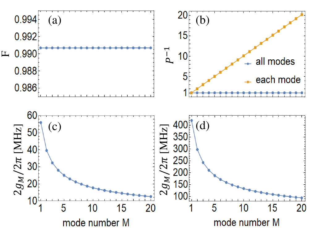
FIG. 6: Fidelities of $|W_{M}\rangle=\frac{1}{M}\sum_{i=1}^{M}|0_{1}0_{2}\cdots 1_{i}0_{i+1}\cdots 0_{M}\rangle$ within the same evolution time for different $M$. a Fidelities of generating $|W_{M}\rangle$ inside resonators in $1$ $\mu$s with $M$ ranging from $1$ to $20$. $\Delta_{1}=\Delta_{2}=0$ MHz , $\Omega=\Omega_{0}exp[-(t-\tau)^{2}/T_{0}^{2}]$, with $\Omega_{0}/2\pi=700$ MHz, $T_{0}=0.36\mu$s, and $\tau=1\mu$s. b Reciprocal of emission probabilities of $|W_{M}\rangle$ (all modes and each mode) into transmission lines in $20$ ns for different $M$. $\kappa/2\pi=500$ MHz. $\Delta_{1}=\Delta_{2}=0$ MHz. $\Omega$ is chosen as Fig. 5c, and $\gamma=\gamma_{\phi}=2\pi\times 0.04$ MHz. c The couplings used to obtain a. $g_{M}=g_{1}/\sqrt{M}$ with $2g_{1}/2\pi=56$ MHz. d The couplings used to obtain b. $g_{M}=g_{1}/\sqrt{M}$ with $2g_{1}/2\pi=420$ MHz.

Next, we consider the emission of such $W$ states through dissipation. By studying the Lindblad master equation including resonator dissipation, qutrit damping and dephasing, we are able to prove the emission rate of the $i$-th resonator $\kappa\langle a_{i}^{\dagger}a_{i}\rangle$ is proportional to $g_{i}^{2}$ when $\kappa_{i}=\kappa$, and an adjustable single-photon multimode $W$ state $|W_{N}\rangle$ could be emitted (see “Methods” section). For its practical usage in quantum information processing, we need to release the $W$ states with high rate and probability. As discussed above, a three-mode $W$ state can be emitted in $20$ ns with probability reaching $98.9\%$. Now we have to find such combinations of parameters for the $N$-mode case.

By analyzing the master equation, we find the total emission rates $\kappa\sum_{i}\langle a_{i}^{\dagger}a_{i}\rangle$ are the same for different mode numbers, under the condition Eq. (8) with other parameters fixed (see “Methods”). For simplicity, we choose $g_{1}=g_{2}=\ldots=g_{N}$, $g_{1^{\prime}}=g_{2^{\prime}}=\ldots=g_{N^{\prime}}$, and reduce Eq. (8) to $Ng_{N}^{2}=N^{\prime}g_{N^{\prime}}^{2}$. Then we choose such couplings varying with mode numbers, as shown in Fig. 6d, where $2g_{1}/2\pi=420$ MHz, and fix other parameters as in the three-mode case where $\kappa/2\pi=500$ MHz, $\gamma=\gamma_{\phi}=2\pi\times 0.04$ MHz, $\Delta_{1}=\Delta_{2}=0$ and $\Omega$ shown in Fig. 5c. The total emission rates and emission probabilities are found to be equal for any mode number $M$ by numerical simulation, where the emission probability $P$ for each mode is naturally $1/M$ of the total emission probability, as shown in Fig. 6b. Now we have found proper parameters to emit the $M$-mode $W$ states in $20$ ns with probability reaching $98.9\%$ for $M$ ranging from $1$ to $20$. This result can be extended to arbitrary $M$ by choosing $g_{M}=g_{1}/\sqrt{M}$ and other parameters fixed.

DISCUSSION

We proposed a unified deterministic scheme of generating and releasing arbitrary single-photon multimode $W$ state on demand with high emission rate and experimental feasibility. We have a qutrit coupled to $N$ spatially separated resonators and a pump pulse. Making the system evolve adiabatically along a dark state, we finally obtain arbitrary $W$ states inside resonators. The first merit of our scheme is the coefficient for the $i$-th basis $|0_{1}0_{2}\cdots 1_{i}0_{i+1}\cdots 0_{N}\rangle$ of this $W$ state is proportional to the coupling strength of the $i$-th mode $g_{i}$, so we can obtain arbitrary $W$ state by changing this coupling. Second, we can release such $W$ states into transmission lines on demand, by adding a variable coupler to modulate the dissipation rate of the resonators. The emission probability reach $98.9\%$ in $20-50$ ns, depending on parameters, comparable to the fastest two-qubit gate. And we only need to vary the pump-laser pulse during the time evolution process, which is easier to control than the qutrit. Third, the generation (or emission) time and fidelity (or probability) can both be the same by choosing $\sum_{i^{\prime}=1}^{N^{\prime}}g^{\prime^{2}}_{i^{\prime}}=\sum_{i=1}^{N}g^{2}_{i}$ and other parameters fixed for $N$-mode and $N^{\prime}$-mode cases. It is interesting to consider its experimental realization in circuit QED or related systems.

METHODS Dark states for generating $|W_{3}\rangle$

The dark state $|\Psi_{0}\rangle$ Eq. (3) is obtained in the interaction picture with respect to free Hamiltonian $H_{0}=E_{u}|u,000\rangle\langle u,000|+(E_{u}+\omega_{P})|e,000\rangle\langle e,000|+(E_{u}+\omega_{P})(|g,100\rangle\langle g,100|+|g,010\rangle\langle g,010|+|g,001\rangle\langle g,001|)$, where the Hamiltonian Eq. (2) reduces to

$$\dfrac{1}{2}\begin{pmatrix}0&\Omega&0&0&0\\ \Omega^{*}&2\Delta_{1}&2g_{1}&2g_{2}&2g_{3}\\ 0&2g_{1}^{*}&2(\Delta_{1}-\Delta_{2})&0&0\\ 0&2g_{2}^{*}&0&2(\Delta_{1}-\Delta_{2})&0\\ 0&2g_{3}^{*}&0&0&2(\Delta_{1}-\Delta_{2})\\ \end{pmatrix},$$ (9)

where $\Delta_{1}=(E_{e}-E_{u})-\omega_{P}$ and $\Delta_{2}=(E_{e}-E_{g})-\omega$. Under the two-photon resonance condition $\Delta_{1}=\Delta_{2}$, there are three degenerate dark states $\{2g_{1}|u,000\rangle-\Omega|g,100\rangle,~{}2g_{2}|u,000\rangle-\Omega|g,010\rangle,~{}2g_{3}|u,000\rangle-\Omega|g,001\rangle\}$ with constant eigenenergy $E=0$, so a general solution with $E=0$ reads:

$$|\Psi_{0}\rangle=\frac{1}{{\cal N}}[2\sum_{i=1}^{3}A_{i}g_{i}|u,000\rangle-\Omega A|g,W_{3}\rangle],$$ (10)

where $A=\sqrt{\sum_{i=1}^{3}A_{i}^{2}}$, $|g,W_{3}\rangle=|g\rangle\otimes|W_{3}\rangle$, $|W_{3}\rangle=\frac{1}{A}(A_{1}|100\rangle+A_{2}|010\rangle+A_{3}|001\rangle)$ and ${\cal N}=\sqrt{4(\sum_{i=1}^{3}{A_{i}g_{i}})^{2}+\Omega^{2}A^{2}}$ is the normalizing constant. The proposed initial state is $|u,000\rangle$, hence $\Omega A_{i}(t=0)=0$. Combined with Schrödinger equation $\frac{{\rm d}(\Omega A_{i})}{{\rm d}t}=-ig_{i}c_{e}$, where $c_{e}=\langle e,000|\psi\rangle$, we obtain $A_{1}:A_{2}:A_{3}=g_{1}:g_{2}:g_{3}$ in this specific situation, and reduce Eq. (10) to $|\Psi_{0}\rangle$ Eq. (3).

Lindblad master equation and emission of $|W_{3}\rangle$

$|W_{3}\rangle$ is released through resonator dissipation, and the dynamics of the system is governed by the Lindblad master equation epjd2010 ; 814 (2010) ; 369 (2002) ; 3140 (2018) ; Oxford Univ. Press (2006) ; 1379 (2015) :

$$\dfrac{d\rho}{dt}=-i[H,\rho]+\sum_{i=1}^{N+2}\dfrac{1}{2}(2L_{i}\rho L_{i}^{\dagger}-L_{i}^{\dagger}L_{i}\rho-\rho L_{i}^{\dagger}L_{i})$$ (11)

where $L_{1}=\sqrt{\kappa_{1}}|g,000\rangle\langle g,100|$, $L_{2}=\sqrt{\kappa_{2}}|g,000\rangle\langle g,010|$, $L_{3}=\sqrt{\kappa_{3}}|g,000\rangle\langle g,001|$, $L_{N+1}=\sqrt{\gamma}(|u,000\rangle\langle e,000|$+$|g,000\rangle\langle e,000|)$, $L_{N+2}=\sqrt{\gamma_{\phi}}(|e,000\rangle\langle e,000|$, and $N$ is the resonator mode number which equals three here. Supposing the system is in state $\rho=\sum p_{m}|\psi_{m}\rangle\langle\psi_{m}|$ with $|\psi_{m}\rangle=c_{um}|u,000\rangle+c_{em}|e,000\rangle+c_{1m}|g,100\rangle+c_{2m}|g010\rangle+c_{3m}|g001\rangle+c_{gm}|g000\rangle$ with $c_{um}=1$ initially and $\kappa_{i}=\kappa$, we find $c_{1m}:c_{2m}:c_{3m}=g_{1}:g_{2}:g_{3}$ is a solution to

$$\dfrac{d(c_{1m}c^{*}_{1m})}{dt} = -ig_{1}(c_{em}c_{1m}^{*}-c_{em}^{*}c_{1m})-\kappa c_{1m}c^{*}_{1m},$$ (12)

$$\dfrac{d(c_{2m}c^{*}_{2m})}{dt} = -ig_{2}(c_{em}c_{2m}^{*}-c_{em}^{*}c_{2m})-\kappa c_{2m}c^{*}_{2m},$$ (13)

$$\dfrac{d(c_{3m}c^{*}_{3m})}{dt} = -ig_{3}(c_{em}c_{3m}^{*}-c_{em}^{*}c_{3m})-\kappa c_{3m}c^{*}_{3m},$$ (14)

such that the master equation Eq. (11) can be satisfied. Therefore, the emission rate of each mode $\kappa Tr(\rho a_{i}^{\dagger}a_{i})$ and its probability $\kappa\int Tr(\rho a_{i}^{\dagger}a_{i})dt$ will be proportional to $g_{i}^{2}$, and a desired $|W_{3}\rangle=\frac{1}{A}(g_{1}|100\rangle_{out}+g_{2}|010\rangle_{out}+g_{3}|001\rangle_{out})$ could be created in the output channels considering $a_{iout}(t)=\sqrt{\kappa}a_{i}(t)$.

Condition for generating $|W_{N}\rangle$ with the same fidelity within the same time for arbitrary $N$

According to the Hamiltonian Eq. (Unified generation and fast emission of arbitrary single-photon multimode $W$ states), the Schrödinger equation gives

$$\dfrac{dc_{u}}{dt} = -\frac{i}{2}\Omega c_{e},$$

$$\dfrac{dc_{e}}{dt} = -\frac{i}{2}(\Omega c_{u}+2\Delta_{1}c_{e}+\sum_{i=1}^{N}2g_{i}c_{i}),$$

$$\dfrac{dc_{i}}{dt} = -ig_{i}c_{e}.$$

It is easy to find if $\sum_{i^{\prime}=1}^{N^{\prime}}g^{\prime^{2}}_{i^{\prime}}=\sum_{i=1}^{N}g^{2}_{i}$, while other parameters are fixed for mode numbers $N$ and $N^{\prime}$, then

$$c^{\prime}_{e}(t) = c_{e}(t),$$ (15)

$$c^{\prime}_{u}(t) = c_{u}(t),$$ (16)

$$c_{i}(t)/c_{j}(t) = g_{i}/g_{j}$$ (17)

$$c_{i^{\prime}}^{\prime}(t)/c_{i}(t) = g_{i^{\prime}}^{\prime}/g_{i}$$ (18)

are solutions of the Schrödinger equation for $N$ and $N^{\prime}$, where $c^{\prime}_{e}(t)$, $c^{\prime}_{u}(t)$ and $c^{\prime}_{i^{\prime}}(t)$ are corresponding wave functions for $N^{\prime}$ case. Therefore, the fidelity to obtain $|W_{N}\rangle$ and $|W_{N^{\prime}}\rangle$ are the same at any time and once we find a combination of parameters to generate a $N$-mode W state with high speed and fidelity, we can easily obtain such parameters for arbitrary $N^{\prime}$ by using Eq. (8).

Then we consider the emission of $|W_{N}\rangle$ using the master equation Eq. (11) with $N$ extended to arbitrary positive integers. First we assume the system is in state $\rho=\sum p_{m}|\psi_{m}\rangle\langle\psi_{m}|$ with $|\psi_{m}\rangle=c_{um}|u,00\ldots 0\rangle+c_{em}|e,00\ldots 0\rangle+\sum_{i=1}^{N}c_{im}|g,00\ldots 1_{i}0_{i+1}0_{N}\rangle+c_{gm}|g00\ldots 0\rangle$ with $c_{um}=1$ initially and $\kappa_{i}=\kappa$. Then following the same routine as the three-mode case, we can prove the emission rate of each resonator $\kappa\langle a_{i}^{\dagger}a_{i}\rangle$ is proportional to $g_{i}^{2}$, and an adjustable single-photon multimode W state could be emitted.

For each $|\psi_{m}\rangle\langle\psi_{m}|$, the master equation Eq. (11) with subscript “m” neglected reads

$$\dfrac{d(c_{i}c^{*}_{i})}{dt} = ig_{i}(c_{e}^{*}c_{i}-c_{e}c_{i}^{*})-\kappa c_{i}c^{*}_{i},$$ (19)

$$\dfrac{d(c_{e}c^{*}_{e})}{dt} = -\frac{i}{2}[\Omega(c_{u}c^{*}_{e}-c_{u}^{*}c_{e})+\sum_{i=1}^{N}2g_{i}(c_{i}c_{e}^{*}-c_{i}^{*}c_{e})]$$ (20)

$$-2\gamma c_{e}c^{*}_{e},$$

$$\dfrac{d(c_{u}c^{*}_{u})}{dt} = -\frac{i}{2}\Omega(c_{e}c^{*}_{u}-c_{e}^{*}c_{u})+\gamma c_{e}c^{*}_{e},$$ (21)

$$\dfrac{d(c_{u}c^{*}_{e})}{dt} = -\frac{i}{2}[\Omega(c_{e}c^{*}_{e}-c_{u}^{*}c_{u})-\sum_{i=1}^{N}2g_{i}c_{u}c_{i}^{*}-2\Delta_{1}c_{u}c^{*}_{e}]$$ (22)

$$-(\gamma+\frac{\gamma_{\phi}}{2})c_{u}c^{*}_{e},$$

$$\dfrac{d(c_{u}c^{*}_{i})}{dt} = -\frac{i}{2}[\Omega c_{e}c^{*}_{i}-2g_{i}c_{u}c_{e}^{*}]-\frac{\kappa}{2}c_{u}c^{*}_{i},$$ (23)

$$\dfrac{d(c_{e}c^{*}_{i})}{dt} = -\frac{i}{2}[\Omega c_{u}c^{*}_{i}+\sum_{j=1}^{N}2g_{j}c_{j}c_{i}^{*}+2\Delta_{1}c_{e}c^{*}_{i}-2g_{i}c_{e}c^{*}_{e}]$$ (24)

$$-(\gamma+\frac{\kappa+\gamma_{\phi}}{2})c_{e}c^{*}_{i},$$

$$\dfrac{d(c_{i}c^{*}_{j})}{dt} = i[g_{j}c_{i}c^{*}_{e}-g_{i}c_{e}c_{j}^{*}]-\kappa c_{i}c^{*}_{j}.$$ (25)

We find Eqs. (15)–(18) are still solutions of the above equation set for different mode numbers $N$ and $N^{\prime}$ under condition $\sum_{i^{\prime}=1}^{N^{\prime}}g^{\prime^{2}}_{i^{\prime}}=\sum_{i=1}^{N}g^{2}_{i}$ and other parameters fixed. The total emission rates $\kappa\sum_{i}^{N}|c_{i}|^{2}$ and $\kappa\sum_{i^{\prime}=1}^{N^{\prime}}|c^{\prime}_{i^{\prime}}|^{2}$ are equal according to Eqs. (8) and (18). So in this specific case, the total emission rate and probability of $|W_{N}\rangle$ and $|W_{N^{\prime}}\rangle$ will be the same at anytime.

DATA AVAILABILITY

The data that support the findings of this study are available from the authors upon reasonable request.

CODE AVAILABILITY

The codes that are used to produce the data presented in this study are available from the authors upon reasonable request.

REFERENCES

- (1) Bennett, C. H. & Wiesner, S. J. Communication via One- and Two-Particle Operators on Einstein-Podolsky-Rosen States. Phys. Rev. Lett. 69, 2881 (1992).
- (2) Bennett, C. H. et al. Teleporting an unknown quantum state via dual classical and Einstein-Podolsky-Rosen channels. Phys. Rev. Lett. 70, 1895 (1993).
- (3) Ekert, A. K. Quantum cryptography based on Bell’s theorem. Phys. Rev. Lett. 67, 661 (1991).
- (4) Grover, L. K. Quantum Mechanics Helps in Searching for a Needle in a Haystack. Phys. Rev. Lett. 79, 325 (1997).
- (5) Einstein, A., Podolsky, B. & Rosen, N. Can Quantum-Mechanical Description of Physical Reality Be Considered Complete? Phys. Rev. 47, 777 (1935).
- (6) Kafatos, M. Bell’s Theorem, Quantum Theory and Conceptions of the Universe (George Mason University press, 1989).
- (7) Yang, C. P., Su, Q. P. & Han, S. Generation of Greenberger-Horne-Zeilinger entangled states of photons in multiple cavities via a superconducting qutrit or an atom through resonant interaction. Phys. Rev. A 86, 022329 (2012).
- (8) Zhang, Y., Liu, T., Zhao, J. L., Yu, Y. & Yang., C. P. Generation of hybrid Greenberger-Horne-Zeilinger entangled states of particlelike and wavelike optical qubits in circuit QED. Phys. Rev. A 101, 062334 (2020).
- (9) Liu, Z. H., Zhou, J., Meng, H. X. et al. Experimental test of the Greenberger–Horne–Zeilinger-type paradoxes in and beyond graph states. npj Quantum Inf 7, 66 (2021).
- (10) Dür, W., Vidal, G. & Cirac, J. I. Three qubits can be entangled in two inequivalent ways. Phys. Rev. A 62, 062314 (2000).
- (11) Ozaydin, F., Bugu, S. N., Yesilyurt, C., Altintas, A. A., Tame, M. & Özdemir Ş. K. Fusing multiple states simultaneously with a Fredkin gate. Phys. Rev. A 89, 042311 (2014).
- (12) Cabello, A. Bell’s theorem with and without inequalities for the three-qubit Greenberger-Horne-Zeilinger and states. Phys. Rev. A 65, 032108 (2002).
- (13) Gangat, A. A., McCulloch I. P., & Milburn G. J. Deterministic Many-Resonator Entanglement of Nearly Arbitrary Microwave States via Attractive Bose-Hubbard Simulation. Phys. Rev. X 3, 031009 (2013).
- (14) Sharma, A. & Tulapurkar, A. A. Generation of n-qubit states using spin torque. Phys. Rev. A 101, 062330 (2020).
- (15) Menotti, M., Maccone, L., Sipe, J. E., & Liscidini, M. Generation of energy-entangled states via parametric fluorescence in integrated devices. Phys. Rev. A 94, 013845 (2016).
- (16) Fang, B., Menotti, M., Liscidini, M., Sipe, J. E. & Lorenz, V. O. Three-Photon Discrete-Energy-Entangled state in an Optical Fiber. Phys. Rev. Lett. 123, 070508 (2019).
- (17) Heo, J., Hong, C., Choi, S. G. & Hong, J. P. Scheme for generation of three-photon entangled state assisted by cross-Kerr nonlinearity and quantum dot. Sci. Rep. 9, 10151 (2019).
- (18) Eibl, M., Kiesel, N., Bourennane, M., Kurtsiefer, C. & Weinfurter, H. Experimental Realization of a Three-Qubit Entangled state. Phys. Rev. Lett. 92, 077901 (2004).
- (19) Zou, X. B., Pahlke, K. & Mathis, W. Generation of an entangled four-photon state. Phys. Rev. A 66, 044302 (2002).
- (20) Dong, L. et al. Nearly deterministic preparation of the perfect state with weak cross-Kerr nonlinearities. Phys. Rev. A 93, 012308 (2016).
- (21) Kim, Y. S., Cho, Y. W., Lim, H. T. & Han, S. W. Efficient linear optical generation of a multipartite state via a quantum eraser. Phys. Rev. A 101, 022337 (2020).
- (22) Peng, J. et. al. One-Photon Solutions to the Multiqubit Multimode Quantum Rabi Model for Fast -State Generation. Phys. Rev. Lett. 127, 043604 (2021).
- (23) Zhang, C. L. & Liu, W. W. Generation of state by combining adiabatic passage and quantum Zeno techniques. Indian J. Phys. 93, 67 (2018).
- (24) Guo, G. P., Li, C. F., Li, J. & Guo, G. C. Scheme for the preparation of multiparticle entanglement in cavity QED. Phys. Rev. A 65, 042102 (2002).
- (25) Deng, Z. J., Feng, M. & Gao, K. L. Simple scheme for generating an n-qubit state in cavity QED. Phys. Rev. A 73, 014302 (2006).
- (26) Guo, G. C. & Zhang, Y. S. Scheme for preparation of the state via cavity quantum electrodynamics. Phys. Rev. A 65, 054302 (2002).
- (27) Wei, X. & Chen, M. F. Generation of -Qubit state in Separated Resonators via Resonant Interaction. Int. J. Theor. Phys. 54, 812 (2015).
- (28) Kang, Y. H., Chen, Y. H., Shi, Z. C., Song, J. & Xia Y. Fast preparation of states with superconducting quantum interference devices by using dressed states. Phys. Rev. A 94, 052311 (2016).
- (29) Kang, Y. H., Chen, Y. H., Wu, Q. C., Huang, B. H., Song, J. & Xia Y. Fast generation of W states of superconducting qubits with multiple Schrödinger dynamics. Sci. Rep. 6, 36737 (2016).
- (30) Stojanović, V. M., Bare-Excitation Ground State of a Spinless-Fermion–Boson Model and W-State Engineering in an Array of Superconducting Qubits and Resonators. Phys. Rev. Lett. 124, 190504 (2020).
- (31) Gangat, A. A., McCulloch, I. P. & Milburn, G. J. Deterministic Many-Resonator W Entanglement of Nearly Arbitrary Microwave States via Attractive Bose-Hubbard Simulation. Phys. Rev. X 3, 031009 (2013).
- (32) Stojanović, V. M., Scalable W-type entanglement resource in neutral-atom arrays with Rydberg-dressed resonant dipole-dipole interaction. Phys. Rev. Lett. 103, 022410 (2021).
- (33) Ozaydin, F., Yesilyurt, C., Bugu, S. N. & Koashi, M. Deterministic preparation of W states via spin-photon interactions. Phys. Rev. A. 103, 052421 (2021).
- (34) Gottesman, D., Jennewein, T. & Croke, S. Longer-Baseline Telescopes Using Quantum Repeaters. Phys. Rev. Lett. 109, 070503 (2012).
- (35) Guha, S. & Shapiro, J. H. Reading boundless error-free bits using a single photon. Phys. Rev. A 87, 062306 (2013).
- (36) Papp, S. B. et al. Characterization of multipartite entanglement for one photon shared among four optical modes. Science 324, 764 (2009).
- (37) Choi, K. S., Goban, A., Papp, S. B., van Enk, S. J. & Kimble, H. J. Entanglement of spin waves among four quantum memories. Nature 468, 412 (2010).
- (38) Li, K., Zheng D. L., Xu, W. Q., Mao, H. B. & Wang, J. Q. states fusion via polarization-dependent beam splitter. Quantum Inf. Process. 19, 412 (2020).
- (39) Gorbachev, V. N., Trubilko, A. I., Rodichkina, A. A. & Zhiliba, A. Can the states of the W-class be suitable for teleportation? Phys. Lett. A 314, 267 (2003).
- (40) Agrawal, P. & Pati, A. Perfect teleportation and superdense coding with states Phys. Rev. A 74, 062320 (2006).
- (41) Li, L. Z. & Qiu, D. W. The states of W-class as shared resources for perfect teleportation and superdense coding. J. Phys. A: Math. Theor. 40, 10871 (2007).
- (42) Sheng, Y. B., Zhou, L. & Zhao, S. M. Efficient two-step entanglement concentration for arbitrary states. Phys. Rev. A 85, 042302 (2012).
- (43) Zhou, L., Sheng, Y. B., Cheng, W. W., Gong, L. Y. & Zhao, S. M. Efficient entanglement concentration for arbitrary single-photon multimode state. J. Opt. Soc. Am. B 30, 71 (2013).
- (44) Yang, C. P., Su, Q. P., Zheng, S. B. & Han, S. Generating entanglement between microwave photons and qubits in multiple cavities coupled by a superconducting qutrit. Phys. Rev. A 87, 022320 (2013).
- (45) Zhang, X. L., Gao, K. L. & Feng, M. Preparation of cluster states and states with superconducting quantum-interference-device qubits in cavity QED. Phys. Rev. A 74, 024303 (2006).
- (46) Deng, Z. J., Gao, K. L. & Feng, M. Generation of -qubit states with rf SQUID qubits by adiabatic passage. Phys. Rev. A 74, 064303 (2006).
- (47) Lu, X. J., Li, M., Zhao, Z. Y., Zhang, C. L., Han, H. P., Feng, Z. B., & Zhou, Y. Q. Nonleaky and accelerated population transfer in a transmon qutrit. Phys. Rev. A 96, 023843 (2017).
- (48) Su, Q. P., Yang, C. P. & Zheng, S. B. Fast and simple scheme for generating NOON states of photons in circuit QED. Sci. Rep. 4, 3898 (2014).
- (49) Liu, Y. H. et. al. Realization of dark state in a three-dimensional transmon superconducting qutrit. Appl. Phys. Lett. 107, 202601 (2015).
- (50) Zhang, Z. X. et. al. Single-shot realization of nonadiabatic holonomic gates with a superconducting Xmon qutrit. New J. Phys. 21 073024 2019.
- (51) Rol, M. A. et. al. Fast, High-Fidelity Conditional-Phase Gate Exploiting Leakage Interference in Weakly Anharmonic Superconducting Qubits. Phys. Rev. Lett. 123, 120502 (2019).
- (52) Kuhn, A., Hennrich, M., Bondo, T. & Rempe, G. Controlled generation of single photons from a strongly coupled atom-cavity system. Appl. Phys. B 69, 373 (1999).
- (53) Xiong, H., Scully, M. O. & Zubairy, M. S. Correlated Spontaneous Emission Laser as an Entanglement Amplifier. Phys. Rev. Lett. 94, 023601 (2005).
- (54) Kuhn, A., Hennrich, M. & Rempe, G. Deterministic Single-Photon Source for Distributed Quantum Networking. Phys. Rev. Lett. 102, 220401 (2009).
- (55) Pechal, M., Huthmacher, L., Eichler, C., Zeytinoğlu, S., Abdumalikov A. A., Jr., Berger, S., Wallraff, A. & Filipp, S. Microwave-Controlled Generation of Shaped Single Photons in Circuit Quantum Electrodynamics. Phys. Rev. X 4, 041010 (2014).
- (56) Bartkowiak, M., Wu, L. A. & Miranowicz, A. Quantum circuits for amplification of Kerr nonlinearity via quadrature squeezing. J. Phys. B 47, 145501 (2014).
- (57) Kiss, T., Herzog, U. & Leonhardt, U. Compensation of losses in photodetection and in quantum-state measurements. Phys. Rev. A 52, 2433 (1995).
- (58) Nielsen, M. A. & Chuang, I. L. in Quantum Computation and Quantum Information (Cambridge University Press, 2000).
- (59) Amin, M. H. S. Consistency of the Adiabatic Theorem. Phys. Rev. Lett. 89, 067901 (2002).
- (60) Yi, Y. et. al. Catch and Release of Microwave Photon States. Phys. Rev. Lett. 110, 107001 (2013).
- (61) Gardiner, C. W. & Collett, M. J. Input and Output in Damped Quantum Systems: Quantum Stochastic Differential Equations and the Master Equation. Phys. Rev. A 31, 3761 (1985).
- (62) Blais, A., Grimsmo, A. L., Girvin, S. M. & Wallraff, A. Circuit quantum electrodynamics. Rev. Mod. Phys. 93, 025005 (2021).
- (63) Baur, M., Filipp, S., Bianchetti, R., Fink, J. M., Göppl, M., Steffen, L., Leek, P. J., Blais A. & Wallraff, A. Measurement of Autler-Townes and Mollow Transitions in a Strongly Driven Superconducting Qubit. Phys. Rev. Lett. 102, 243602 (2009).
- (64) Law, C. K. & Kimble H. J. Deterministic generation of a bit-stream of single-photon pulses. J. Mod. Opt. 44, 2067 (1997).
- (65) Mlynek, J. A., Abdumalikov, A. A., Eichler, C. & Wallraff, A. Observation of Dicke superradiance for two artificial atoms in a cavity with high decay rate. Nat. Commun. 5, 5186 (2014).
- (66) Hu, M. L. State transfer in dissipative and dephasing environments. Eur. Phys. J. D 59, 497 (2010).
- (67) Li, G. X. & Ficek, Z. Creation of pure multi-mode entangled states in a ring cavity. Opt. Commun. 283, 814 (2010).
- (68) Ficeka, Z. & Tanaś, R. Entangled states and collective nonclassical effects in two-atom systems. Phys. Rep. 372, 369 (2002).
- (69) Zhang, X., Xu, C. & Ren, Z. Z. High fdelity heralded singlephoton source using cavity quantum electrodynamics Sci. Rep. 8, 3140 (2018).
- (70) Haroche, S. & Raimond, J. M. Exploring the Quantum: Atoms, Cavities and Photons, (Oxford University Press, 2006).
- (71) Reiserer, A. & Rempe, G. Cavity-based quantum networks with single atoms and optical photons. Rev. Mod. Phys. 87, 1379–1418 (2015). ACKNOWLEDGEMENTS This work was supported by the Scientific Research Fund of Hunan Provincial Education Department (18A436), Natural Science Foundation of Hunan Province, China (2016JJ6020,2018JJ3482), the National Basic Research Program of China (2015CB921103), the Program for Changjiang Scholars and Innovative Research Team in University (No. IRT13093), and the National Natural Science Foundation of China (11704320). AUTHOR CONTRIBUTIONS J.C.Z. and J.P. designed the project and conducted analytical derivation. J.C.Z., J.P. and P.H.T. analyzed the numerical data and wrote the paper with inputs from F.L. and N.T. All authors discussed the results and contributed to the final paper. COMPETING INTERESTS The authors declare that there are no competing interests. ADDITIONAL INFORMATION Correspondence and requests for materials should be addressed to J.P. or J.C.Z.