Moving average options: Machine Learning and Gauss-Hermite quadrature for a double non-Markovian problem

Abstract

Evaluating moving average options is a tough computational challenge for the energy and commodity market as the payoff of the option depends on the prices of a certain underlying observed on a moving window so, when a long window is considered, the pricing problem becomes high dimensional. We present an efficient method for pricing Bermudan style moving average options, based on Gaussian Process Regression and Gauss-Hermite quadrature, thus named GPR-GHQ. Specifically, the proposed algorithm proceeds backward in time and, at each time-step, the continuation value is computed only in a few points by using Gauss-Hermite quadrature, and then it is learned through Gaussian Process Regression. We test the proposed approach in the Black-Scholes model, where the GPR-GHQ method is made even more efficient by exploiting the positive homogeneity of the continuation value, which allows one to reduce the problem size. Positive homogeneity is also exploited to develop a binomial Markov chain, which is able to deal efficiently with medium-long windows. Secondly, we test GPR-GHQ in the Clewlow-Strickland model, the reference framework for modeling prices of energy commodities. Finally, we consider a challenging problem which involves double non-Markovian feature, that is the rough-Bergomi model. In this case, the pricing problem is even harder since the whole history of the volatility process impacts the future distribution of the process. The manuscript includes a numerical investigation, which displays that GPR-GHQ is very accurate and it is able to handle options with a very long window, thus overcoming the problem of high dimensionality.

Declarations of interest: none.

1 Introduction

In this manuscript, we are interested in path-dependent options whose payoff depends on the average of the prices of a certain underlying, observed in a sliding window. Options on the moving average price are widespread in the commodities sector and in particular in the gas and oil market. In this context, these options are known as “swing options” (see, e.g. Bernhart et al., [5]) and allow the holder to buy a certain amount of gas or oil at the average price observed in a certain window, in order to compensate for possible anomalous peaks in prices: for example, the average of the daily closing prices of the last month or of the last week. Furthermore, moving average options are also popular in corporate finance, where they are used to protect a company from hostile acquisitions (see, e.g. Dai et al., [10]).

The payoff of moving average options depends on the average of a fixed number of the last observed daily closing prices. Usually, the moving window can include from a few days to a few tens (Kao and Lyuu, [21], Bernhart et al., [5]). These options are similar to Asian options, whose payoff depends on the average price of the underlying, calculated from the inception time to the exercise time. However, the valuation of Asian options is relatively simple since, under standard assumptions, the average over the entire time interval and the underlying price define a Markov process. On the contrary, the sliding window feature of the moving average options makes their evaluation much more complicated as the moving average and the underlying do not define a Markov process: the price of the option is a function of every single value that is used to compute the average, and therefore a function of a potentially large number of variables.

Pricing American-style moving average options has garnered the attention of several authors. The approaches proposed in this regard are of three types essentially. The first group of methods includes Longstaff-Schwartz type approaches, which is a state-of-the-art approach in the energy sector (see, e.g. Nadarajah et al., [25]). One of the first attempts in this field is due to Bilger, [6], which uses a standard Longstaff-Schwartz method. Grau, [19] improves the numerical efficiency of such an approach by using a sparse polynomial basis for the regression. Broadie and Cao, [7] propose to use polynomials of the underlying index and the average, as well as to exploit two variance reduction techniques to improve convergence. Bernhart et al., [5] propose a method based on Laguerre polynomial approximation to price the continuously monitored moving average options. Dirnstorfer et al., [12] exploit sparse grid basis functions based on polynomials or piecewise linear functions. More recently, Lelong, [22] introduces a Longstaff-Schwartz type approach in which the standard least-square regression is replaced by a Wiener chaos expansion.

The second group includes techniques based on partial differential equations (PDE). Dai et al., [10] introduce an algorithm for pricing discretely monitored moving average barrier options based on the resolution of a PDE and obtain the price of continuously monitored option by Richardson’s extrapolation. Federico and Tankov, [15] study from a theoretical perspective stochastic delay differential equations which may be used for computing the price of moving average options.

The third group involves techniques that rely on lattices, which is common approach to price options on averages (see, e.g. Costabile et al., [9], Gambaro et al., [17]). Kao and Lyuu, [21] present pricing algorithms based on the CRR binomial model for geometric and arithmetic moving-average type options. Xu et al., [28] propose a sampling strategy that improves willow trees. Lu et al., [23] propose two willow tree methods for pricing European-style and American-style moving average barrier options.

Finally, it is worth mentioning the works of Dong and Kang, [13, 14] who study a particular type of swing contracts that include a moving average feature, by means of a two-dimensional trinomial tree and least squares Monte Carlo methods. To conclude this review, we also mention the research on the dynamic hedging of moving average options of Warin, [27].

The previously mentioned works consider moving average options with a moving window that includes at most 10 observations (see Dirnstorfer et al., [12], Bernhart et al., [5], Lelong, [22]). The difficulty in going beyond this number of observations is due to the computational complexity of the problem. When the average is computed on many observations, the evaluation of American-style moving average options becomes a high dimensional problem which suffers from the well-known curse of dimensionality.

In the last few years, Gaussian Process Regression (GPR), a Machine Learning technique that allows estimations from a certain number of observed values, has recently been used to face high-dimensional problems in finance. In this regard, we mention the work of Ludkovski, [24], who evaluates Bermudan options by fitting the continuation values through GPR and De Spiegeleer et al., [11], that exploit GPR to speed up derivative pricing by using an online-offline approach. More recently, Goudenège et al., [18] employ GPR for pricing American options on a basket of assets following multi-dimensional Black-Scholes dynamics.

In this paper, we show how to approach the evaluation of high-dimensional Bermudan moving average options by using GPR and Gauss-Hermite quadrature. Specifically, we propose a method, called GPR-GHQ, that works by moving backward in time. At each time step, the continuation value is computed only for some quasi-random data points, which represent some possible observed values of the underlying, by using Gauss-Hermite quadrature (see, e.g. Judd, [20]). Then, following the same approach of Ludkovski, [24] and Goudenège et al., [18], we exploit GPR to learn the continuation value of the moving average option from the few observed values. First of all, we focus on the Black-Scholes model. In this particular case, the continuation value is a positive homogeneous function of observed underlying values and such a property can be exploited to reduce by one the dimension of the problem. Moreover, such a feature also allows us to define an efficient pricing model based on a binomial Markov chain, which turns out to be particularly efficient for medium-high dimensional options. Since moving average options are also used in the energy markets, we also test the GPR-GHQ method in the Clewlow-Strickland model for prices of energy commodities, which is able to match the forward curve and also provides mean reversion. Recently Alfeus and Sklibosios Nikitopoulos, [2] show that the volatility in the commodity market is rough, therefore we also consider the rough-Bergomi model, introduced by Bayer et al., [3], which is a promising rough volatility model in quantitative finance. This latter model is particularly interesting as the underlying is as a process with fractional stochastic volatility. Therefore, in this case, we face a double non-Markovian option pricing problem: the absence of Markov property is due both to the underlying process, which has volatility with memory, and to the moving average, which is not a Markov process even in the simplest stochastic models, as it depends on all underlying values included in the moving window. We present numerical results for all the three stochastic models mentioned above and we perform an empirical convergence analysis to show that the proposed method outperforms the standard Longstaff-Schwartz algorithm and it is very accurate and efficient in handling high dimensional moving average options.

The remainder of the paper is organized as follows. In Section 2 we present the considered stochastic models. In Section 3 we present moving average options. In Section 4 we outline the main features of the GPR-GHQ method. In Section 5 we discuss the binomial chain method. In Section 6 we present and discuss the results of the numerical simulations. In Section 7 we conclude.

2 The stochastic models

In this paper we consider three stochastic models, namely the Black-Scholes model, the Clewlow-Strickland model and the rough-Bergomi model. In order to fix the notation, we report models dynamics under a risk neutral probability $\mathbb{P}$. Simulation procedure for the rough-Bergomi model is outlined in the A, while for the other two models, we refer the interested reader, e.g., to Fusai and Roncoroni, [16].

2.1 The Black-Scholes model

The Black-Scholes model is widely recognized as one of the most important models in finance. It models the dynamics of a stock price by the following stochastic differential equation (SDE):

$$\frac{dS_{t}}{S_{t}}=r\,dt+\sigma\,dB_{t},$$ (2.1)

with $r$ the risk free interest rate, $\sigma$ the volatility and $\left(B_{t}\right)_{t\in\left[0,T\right]}$ a Brownian motion.

2.2 The Clewlow-Strickland model

The Clewlow-Strickland model [8] is the standard model for commodity price dynamics. Let $S_{t}$ be the spot price of a commodity and let $F\left(t,T\right)$ denote its forward price at time $t\in\left[0,T\right]$ with maturity $T$. The model assumes that $F\left(t,T\right)$ is the solution of the following SDE

$$\frac{dF(t,T)}{F(t,T)}=\sigma e^{-\alpha(T-t)}dB_{t},$$ (2.2)

with $\alpha$ and $\sigma$ positive constants and $\left(B_{t}\right)_{t\in\left[0,T\right]}$ a Brownian motion. Starting from (2.2), one can prove that the spot price is given by the following relation

$$S_{t} =F(0,t)\exp\left[\frac{\sigma^{2}}{4\alpha}\left(e^{-2\alpha t}-1\right)+\int_{0}^{t}\sigma e^{-\alpha(t-u)}dB_{u}\right].$$ (2.3)

2.3 The rough-Bergomi model

The rough-Bergomi model is a non-Markovian model, recently introduced by Bayer et al., [3], that provides stochastic volatility with memory and it is appreciated as it generates a realistic term structure of at-the-money volatility skew. The model is described by the following SDE:

$$\begin{cases}dS_{t}&=rS_{t}dt+\sqrt{V_{t}}S_{t}dB_{t}^{1}\\ V_{t}&=\xi_{0}\left(t\right)\exp\left(\eta\widetilde{B}_{t}^{H}-\frac{1}{2}\eta^{2}t^{2H}\right),\end{cases}$$

with $r$ the risk free interest rate, $\eta$ a positive parameter, $H\in\left]0,1\right[$ the Hurst parameter and $\xi_{0}\left(t\right)$ a deterministic function that models the forward variance curve. The process $B_{t}^{1}$ is a Brownian motion, whereas $\widetilde{B}_{t}^{H}$ is a Riemann-Liouville fractional Brownian motion, a non-Markovian process that can be expressed as

$$\widetilde{B}_{t}^{H}=\sqrt{2H}\int_{0}^{t}\left(t-s\right)^{H-\frac{1}{2}}dB_{t}^{2},$$ (2.4)

with $B_{t}^{2}$ a Brownian motion and $\rho$ the instantaneous correlation coefficient between $B_{t}^{1}$ and $B_{t}^{2}$.

3 Moving average options

We consider a time interval $\left[0,T\right]$ and a stochastic process $\left(S_{t}\right)_{t\in\left[0,T\right]}$ that models a market index, for example the price of a stock or of a commodity. Let us suppose that there are $N$ trading dates $t_{1},\dots t_{N}$ in $\left]0,T\right]$ with $t_{n}=\nicefrac{{nT}}{{N}}$, so that $t_{N}=T$. Let $n_{1},n_{2}$ be two integers with $0\leq n_{1}\leq n_{2}\leq N$, and let $A_{n_{1}}^{n_{2}}$ represent the average closing value of the process $S$ form $t_{n_{1}}$ to $t_{n_{2}}$, that is

$$A_{n_{1}}^{n_{2}}=\frac{1}{n_{2}-n_{1}+1}\sum_{j=n_{1}}^{n_{2}}S_{t_{j}}.$$

We stress out that $A_{n}^{n}=S_{t_{n}}$. The payoff of a moving average option at time $t_{n}$ is given by

$$\Psi\left(S_{t_{n-M+1}},S_{t_{n-M+2}},\dots,S_{t_{n}}\right)=\max\left(0,S_{t_{n}}-A_{n-M+1}^{n}\right),$$ (3.1)

with $M$ the number of observed underlying values included in the average. Please observe that, since the first available underlying value is $S_{0}$, the payoff function can not be evaluated before time $t_{M-1}$.

We are interested in Bermudan options, which can be exercised at any time step $t_{n}$, for $n=M,\dots,N$. It is worth underlying that, following Bernhart et al., [5] and Lelong, [22], the first time the option can be exercises is $t_{M}$, but other choices are possible.

Although this type of option may have the appearance of an Asian call with a floating strike, there is a very important difference. Unlike what happens for Asian options, the pair $\left(S_{t_{n}},A_{n-M+1}^{n}\right)_{n=M,\dots,N}$ does not define a Markov process, even if $\left(S_{t_{n}}\right)_{n=M,\dots,N}$ is a Markov process. In fact, the updating rule for $A$ is given by

$$A_{\left(n+1\right)-M+1}^{\left(n+1\right)}=A_{n-M+1}^{n}+\frac{S_{t_{n+1}}-S_{t_{n-M+1}}}{M},$$ (3.2)

so that the distribution law of the couple $\left(S_{t_{n+1}},A_{n+1-M+1}^{n+1}\right)$ does not depend only on $\left(S_{t_{n}},A_{n-M+1}^{n}\right)$ but also on $S_{t_{n-M+1}}$. That is because the averaging window moves with time and so the oldest underlying value included in the average has to be removed from the average to leave room for the newest underlying value. By exploiting a similar reasoning, one can show that the distribution law of $\left(S_{t_{n+2}},A_{\left(n+2\right)-M+1}^{\left(n+2\right)}\right)$ depends on $S_{t_{n-M+2}}$ and so on, so that all the $M$ values $S_{t_{n-M+1}},S_{t_{n-M+2}},\dots,S_{t_{n}}$ are required to write the law of the couple $\left(S_{t_{k}},A_{k-M+1}^{k}\right)$ for any $k$ in $\left\{n+1,\dots,n+M\right\}$. So, Kao and Lyuu, [21] suggests to use the moving window process $\left(\mathbf{S}_{n}\right)_{n=M,\dots,N}$ defined as

$$\mathbf{S}_{n} =\left(\mathbf{S}_{n,1},\mathbf{S}_{n,2},\dots,\mathbf{S}_{n,M}\right)^{\top}=\left(S_{t_{n-M+1}},\dots,S_{t_{n}}\right)^{\top},$$

which is Markovian, although process $\left(S_{t_{n}},A_{n-M+1}^{n}\right)$ is not, and $A_{n-M+1}^{n}$ is measurable with respect to $\mathbf{S}_{n}$.

Here we prefer to consider a different approach. Specifically, we describe the moving average option in terms of the process of the last partial averages $\left(\mathbf{A}_{n}\right)_{n=M,\dots,N}$, which writes

$$\mathbf{A}_{n} =\left(\mathbf{A}_{n,1},\mathbf{A}_{n,2},\dots,\mathbf{A}_{n,d_{n}^{A}}\right){}^{\top}=\left(A_{n-M+1}^{n},A_{n-M+2}^{n},\dots,A_{\min\left\{n-1,N-M+1\right\}}^{n},A_{n}^{n}\right)^{\top}.$$

For example, if $M=2$, then $\mathbf{A}_{n}=\left(A_{n-1}^{n},\dots,A_{\min\left\{n-1,N-1\right\}}^{n},A_{n}^{n}\right)^{\top}$, thus $\mathbf{A}_{N}=\left(A_{N-1}^{N},A_{N}^{N}\right)^{\top}$, $\mathbf{A}_{N-1}=\left(A_{N-2}^{N-1},A_{N-1}^{N-1}\right)^{\top}$ and $\mathbf{A}_{N-2}=\left(A_{N-3}^{N-2},A_{N-2}^{N-2}\right)^{\top}$, while if $M=3$, then $\mathbf{A}_{n}=\left(A_{n-2}^{n},\dots,A_{\min\left\{n-1,N-2\right\}}^{n},A_{n}^{n}\right)^{\top}$, thus $\mathbf{A}_{N}=\left(A_{N-2}^{N},A_{N}^{N}\right)^{\top}$, $\mathbf{A}_{N-1}=\left(A_{N-3}^{N-1},A_{N-2}^{N-1},A_{N-1}^{N-1}\right)^{\top}$ and $\mathbf{A}_{N-2}=\left(A_{N-4}^{N-2},A_{N-3}^{N-2},A_{N-2}^{N-2}\right)^{\top}$.

Let us point out some properties of the process $\mathbf{A}$. The dimension changes with time and, at time $t_{n}$, it is equal to $d_{n}^{A}=\min\left\{M,N-n+2\right\}$ which means it increases by one unit moving backward in time up to $t_{N-M+2}$ when it is equal to $M$ and stops augmenting. Specifically, the last component is $A_{n}^{n}=S_{t_{n}}$, while the first component is the average of the last $M$ observed underlying values, the second one is the average of the last $M-1$ observed underlying values and so on. Generally speaking, the $i$-th component $\mathbf{A}_{n,i}$ is equal to the mean of the last $M+1-i$ observed underlying values, with the exception of the last component $\mathbf{A}_{n,d_{n}}$ which is the last observed price, that is $S_{n}$. If $S$ is Markovian, then $\mathbf{A}$ is Markovian too. In fact, $A_{n}^{n}=S_{t_{n}}$ and

$$A_{n+1}^{n+1} =S_{t_{n+1}},$$ (3.3)

$$A_{i}^{n+1} =\frac{\left(n-i+1\right)A_{i}^{n}+S_{t_{n+1}}}{n-i+2},$$ (3.4)

or equivalently, with respect to the components of $\mathbf{A}$, we have

$$\mathbf{A}_{n+1,i}=\begin{cases}S_{t_{n+1}}&\text{if }i=d_{n+1}^{A}\\ \frac{\left(M-i\right)\mathbf{A}_{n,i+1}+S_{t_{n+1}}}{M+1-i}&\text{otherwise. }\end{cases}$$ (3.5)

We emphasize that the payoff of the option is measurable with respect to process $\mathbf{A}$, so let us denote with $\Psi_{n}^{\mathbf{A}}$ the payoff as a function of the process $\mathbf{A}_{n}$, that is

$$\Psi_{n}^{\mathbf{A}}\left(A_{n}\right)=\Psi_{n}^{\mathbf{A}}\left(A_{n-M+1}^{n},A_{n-M+2}^{n},\dots,A_{\min\left\{n-1,N-M+1\right\}}^{n},A_{n}^{n}\right)=\max\left(0,A_{n}^{n}-A_{n-M+1}^{n}\right).$$ (3.6)

The use of the process $\mathbf{A}$ in place of the process $\mathbf{S}$ brings computational advantages since, while process $\mathbf{S}$ is $M$-dimension, process $\mathbf{A}$ has dimension at most $M$, so it speeds up calculations, in particular regression, which is a key part in the GPR-GHQ method.

4 The GRP-GHQ method

The method we propose is called GPR-GHQ as it employs the Gaussian Process Regression (GPR) method and the Gauss-Hermite (GHQ) quadrature scheme.

GPR is a non-parametric Bayesian method for regression that belongs to the group of machine learning techniques. In the B we report a brief description of such an approach. We use this technique as GPR has several advantages over other similar techniques such as neural networks: it works well on small data sets and has the ability to provide uncertainty measurements on predictions.

Finally, GHQ is a famous technique in option pricing, so we simply present a brief description of it in C.

4.1 The algorithm for the Black-Scholes model

The GPR-GHQ method is a backward induction algorithm that employs GHQ to compute the continuation value of the option only for some particular path of the underlying and it employs GPR to extrapolate the whole continuation value from those observations. First of all, we present the method for the Black-Scholes model and then we discuss how to adapt it to the Clewlow-Strickland model and to the rough-Bergomi model. So, let us suppose that the underlying follows the Black-Scholes dynamics.

Let $N$ denote the number of time steps, $\Delta t=T/N$ be the time increment and $t_{n}=n\,\Delta t$ represent the discrete time steps for $n=0,1,\ldots,N$ as in Section 3. In order to price the Bermudan moving average option, we consider the process $\left(\mathbf{B}_{n}\right)_{n=M,\dots,N}$, which writes

$$\mathbf{B}_{n} =\left(\mathbf{B}_{n,1},\mathbf{B}_{n,2},\dots,\mathbf{B}_{n,d_{n}^{B}}\right){}^{\top}=\left(A_{n-M+2}^{n},A_{n-M+3}^{n},\dots,A_{\min\left\{n-1,N-M+1\right\}}^{n},A_{n}^{n}\right)^{\top},$$ (4.1)

which can be obtained by $\mathbf{A}_{n}$ by dropping the first component $\mathbf{A}_{n,1}$, that is $A_{n-M+1}^{n}$ (thus, the dimension of $\mathbf{B}_{n}$ is $d_{n}^{B}=d_{n}^{A}-1)$. We compute the option price by moving backward in time and by computing the option value only at time steps $t_{n}$ with $n\in\left\{M,\dots,N\right\}$. Specifically, the option value $\mathcal{V}_{n}$ at time $t_{n}$ is determined by the process of partial averages $\mathbf{A}_{n}$ as follows:

$$\mathcal{V}_{n}\left(\mathbf{A}_{n}\right)=\max\left(\Psi_{n}^{\mathbf{A}}\left(\mathbf{A}_{n}\right),\mathcal{C}_{n}\left(\mathbf{B}_{n}\right)\right),$$ (4.2)

with $\mathcal{C}_{n}$ the continuation value function of the moving average option at time $t_{n}$ which is given by the following relation

$$\mathcal{C}_{n}\left(\mathbf{B}_{n}\right)=\mathbb{E}_{t_{n},\mathbf{B}_{n}}\left[e^{-r\Delta t}\mathcal{V}_{n+1}\left(\mathbf{A}_{n+1}\right)\right].$$ (4.3)

where $\mathbb{E}_{t_{n},\mathbf{B}_{n}}$ represents the expectation at time $t_{n}$ given that $\mathbf{B}_{n}$ is the value of the process $\mathbf{B}$ at time $t_{n}$. Please observe that the law of $\mathbf{A}_{n+1}|\mathbf{A}_{n}$ is the same as $\mathbf{A}_{n+1}|\mathbf{B}_{n}$ because, according to (3.5), $\mathbf{A}_{n,1}$ is not used to obtain $\mathbf{A}_{n+1}$, so we can consider the conditional expectation $\mathbb{E}_{t_{n},\mathbf{B}_{n}}$ that requires less information with respect to $\mathbb{E}_{t_{n},\mathbf{A}_{n}}$ (so it is more convenient from a computational perspective) and we write $\mathcal{C}_{n}$ as a function of $\mathbf{B}_{n}$ in place of $\mathbf{A}_{n}$ . Moreover, the following equation points out the relation between $\mathbf{A}_{n+1}$ and $\mathbf{B}_{n+1}$

$$\mathbf{A}_{n+1}=\left(\frac{\left(M-1\right)\mathbf{B}_{n,1}+\mathbf{B}_{n+1,d_{n+1}^{B}}}{M},\mathbf{B}_{n+1}\right),$$ (4.4)

so that one can obtain $\mathbf{A}_{n+1}$ from $\mathbf{B}_{n}$ and $\mathbf{B}_{n+1}$.

We stress out that the continuation value at maturity is zero, since the option expiry after time $T$, that is

$$\mathcal{C}_{N}\left(\mathbf{B}_{N}\right) = 0$$ (4.5)

an obviously

$$\mathcal{V}_{N}\left(\mathbf{A}_{N}\right)=\Psi_{N}^{\mathbf{A}}\left(\mathbf{A}_{N}\right).$$

Thus, we can observe that the continuation value at time $t_{N-1}$ simplifies as follows

$$\mathcal{C}_{N-1}\left(\mathbf{B}_{N-1}\right) =\mathbb{E}_{t_{N-1},\mathbf{B}_{N-1}}\left[e^{-r\Delta t}\Psi_{N}^{\mathbf{A}}\left(\mathbf{A}_{N}\right)\right]$$

$$=\mathbb{E}_{t_{N-1},\mathbf{B}_{N-1}}\left[e^{-r\Delta t}\max\left(0,S_{T}-\frac{1}{M}\sum_{j=N-M+1}^{N}S_{t_{j}}\right)\right]$$

$$=\mathbb{E}_{t_{N-1},\mathbf{B}_{N-1}}\left[e^{-r\Delta t}\max\left(0,\frac{M-1}{M}S_{T}-\frac{1}{M}\sum_{j=N-M+1}^{N-1}S_{t_{j}}\right)\right]$$

$$=\frac{M-1}{M}\mathbb{E}_{t_{N-1},\mathbf{B}_{N-1}}\left[e^{-r\Delta t}\max\left(0,S_{T}-\frac{1}{M-1}\sum_{j=N-M+1}^{N-1}S_{t_{j}}\right)\right]$$

$$=\frac{M-1}{M}\mathbb{E}_{t_{N-1},\mathbf{B}_{N-1}}\left[e^{-r\Delta t}\max\left(0,S_{T}-\frac{MA_{N-1-M+2}^{N-1}}{M-1}\right)\right]$$

$$=\frac{M-1}{M}\mathcal{C}all\left(t_{N-1},t_{N},A_{N-1}^{N-1},\frac{MA_{N-1-M+2}^{N-1}}{M-1}\right),$$ (4.6)

where $\mathcal{C}all\left(t_{0},T,S_{0},K\right)$ stands for the price of a European call option on $S$ with inception time $t_{0}$, maturity $T$, spot value $S_{0}$, and strike $K$.

By exploiting equations (4.5), (4.6) and (4.2), we can write a dynamic programming problem of the function $C$ as follows:

$$\begin{cases}\mathcal{C}_{N}\left(\mathbf{B}_{N}\right)&=0\\ \mathcal{C}_{N-1}\left(\mathbf{B}_{N-1}\right)&=\mathcal{C}all\left(t_{N-1},t_{N},A_{N-1}^{N-1},\frac{MA_{n-M+1}^{n}-A_{n}^{n}}{M-1}\right)\\ \mathcal{C}_{n}\left(\mathbf{B}_{n}\right)&=\mathbb{E}_{t_{n},\mathbf{B}_{n}}\left[e^{-r\Delta t}\max\left(\Psi_{n+1}^{A}\left(\mathbf{A}_{n+1}\right),\mathcal{C}_{n+1}\left(\mathbf{B}_{n+1}\right)\right)\right],\ \text{for}\ n=N-2,\dots,M.\end{cases}$$ (4.7)

So, by simply computing the price of a European Call option, the continuation value can be evaluated at time $t_{N}$ and $t_{N-1}$,

Now, we aim to solve problem (4.7) by moving backward in time, starting from $t_{N-1}$ up to $t_{M}$. The key point is that, for $n=N-2,\dots,M$, the continuation value is the expectation of the random variable

$$e^{-r\Delta t}\max\left(\Psi_{n+1}^{A}\left(\mathbf{A}_{n+1}\right),\mathcal{C}_{n+1}\left(\mathbf{B}_{n+1}\right)\right)|\mathbf{B}_{n},$$

which is measurable once the value of the one-dimensional random variable $S_{t_{n+1}}$ is known. Therefore, if one can evaluate the function $\mathcal{C}_{n+1}$, then $\mathcal{C}_{n}$ can be computed efficiently at any point by means of a one-dimensional quadrature formula which is a very efficient method. By iterating the same reasoning, if the function $\mathcal{C}_{n}$ can be computed at any point, one can also compute $\mathcal{C}_{n-1}$ and the procedure can repeat up to $t_{M}$. However, if the evaluation of $\mathcal{C}_{n}$ at any point exploits directly a quadrature formula, then the evaluation of $\mathcal{C}_{n-1}$ , which depends on $\mathcal{C}_{n}$, would require a two nested quadrature formulas. Similarly, evaluating $\mathcal{C}_{n-2}$ would require three nested quadrature formulas, so that the computational cost explodes in a few time steps. In order to overcome such a problem, we exploit GPR to learn $\mathcal{C}_{n}$ from a few observed value, so that evaluating $\mathcal{C}_{n}$ at any point becomes very fast as it relies directly on GPR.

First of all, we need to select some points where evaluate the function $\mathcal{C}_{n}$ and employ those observations as the training set for GPR. To this aim, we employ a quasi-random generator, for example the Halton sequence, to simulate $P$ discrete time paths for the process $S$ and thus for $\mathbf{A}$ and $\mathbf{B}$.

Let us consider a time step $t_{n}$ and suppose that the continuation value $\mathcal{C}_{n}$ is known, at least in an approximate form, at time $t_{n+1}$. Our target is to obtain an approximation for $\mathcal{C}_{n}$. To this aim, we consider a set $X^{n}$ of $P$ points whose elements are the simulated values for $\mathbf{B}_{n}$:

$$X^{n}=\left\{\mathbf{x}^{n,p}=\left(x_{1}^{n,p},\dots,x_{d_{n}^{B}}^{n,p}\right),p=1,\dots,P\right\}\subset\mathbb{R}^{d_{n}}.$$ (4.8)

The GPR-GH method assesses $\mathcal{C}_{n}\left(\mathbf{x}^{n,p}\right)$ for each $\mathbf{x}^{n,p}\in X^{n}$ through $Q$-points GHQ. Specifically, let $\left\{u_{q}\right\}_{q=1,\dots,Q}$ and $\left\{w_{q}\right\}_{q=1,\dots,Q}$ be the GHQ nodes and weights. The last component of $\mathbf{x}^{n,p}$, i.e. $x_{d_{n}^{B}}^{n,p}$, corresponds to the value $S_{t_{n}}$, so $Q$ possible determinations for $S_{t_{n+1}}|S_{t_{n}}=x_{d_{n}^{B}}^{n,p}$ are employed by GHQ, precisely,

$$S^{n,p,q}=x_{d_{n}}^{n,p}\cdot\exp\left(\left(r-\frac{\sigma^{2}}{2}\right)\Delta t+u_{q}\sqrt{2\Delta t}\sigma\right),\ q=1,\dots,Q.$$

So, there also are $Q$ possible determinations for $\mathbf{B}_{n+1}|\mathbf{B}_{n}=\mathbf{x}^{n,p}$, specifically

$$\tilde{X}^{n,p}=\left\{\mathbf{\mathbf{\tilde{x}}}^{n,p,q}=\left(\tilde{x}_{1}^{n,p,q},\dots,\tilde{x}_{d_{n+1}^{B}}^{n,p,q}\right)\right\}_{q=1\dots Q},$$

with

$$\tilde{x}_{d_{n+1}}^{n,p,q}=S^{n,p,q},$$

and by exploiting relation (3.5), we can write

$$\tilde{x}_{i}^{n,p,q}=\frac{\left(M-i-1\right)x_{i+1}^{n,q}+S^{n,p,q}}{M-i}.$$

We also define

$$\tilde{x}_{0}^{n,p,q}=\frac{\left(M-1\right)x_{1}^{n,q}+S^{n,p,q}}{M},$$

so that the vector $\left(\tilde{x}_{0}^{n,p,q},\mathbf{\mathbf{\tilde{x}}}^{n,p,q}\right)$ is a possible outcome for $\mathbf{A}_{n+1}|\mathbf{B}_{n}=\mathbf{x}^{n,p}$, thanks to (4.4). Then, the continuation value at $\mathbf{x}^{n,p}$, that is

$$\mathcal{C}_{n}\left(\mathbf{x}^{n,p}\right)=\mathbb{E}_{t_{n},\mathbf{x}^{n,p}}\left[e^{-r\Delta t}\max\left(\Psi_{n+1}^{A}\left(\mathbf{A}_{n+1}\right),\mathcal{C}_{n+1}\left(\mathbf{B}_{n+1}\right)\right)\right],$$

is approximated by

$$\mathcal{C}_{n}^{GHQ}\left(\mathbf{x}^{n,p}\right)=e^{-r\Delta t}\sum_{q=1}^{Q}w_{q}\max\left(\Psi_{n+1}^{A}\left(\tilde{x}_{0}^{n,p,q},\mathbf{\mathbf{\tilde{x}}}^{n,p,q}\right),\mathcal{C}_{n+1}\left(\mathbf{\mathbf{\tilde{x}}}^{n,p,q}\right)\right).$$ (4.9)

Equation (4.9) can be evaluated only if the quantities $\mathcal{C}_{n+1}\left(\mathbf{\mathbf{\tilde{x}}}^{n,p,q}\right)$ are known for all the future points $\mathbf{\mathbf{\tilde{x}}}^{n,p,q}$. As pointed out in (4.7), both the functions $\mathcal{C}_{N}$ and $\mathcal{C}_{N-1}$ are known, so one can employ (4.9) to compute $\mathcal{C}_{N-2}^{GHQ}\left(\mathbf{x}^{N-2,p}\right)$ for all $\mathbf{x}^{N-2,p}$ in $X^{N-2}$. In order to compute $\mathcal{C}_{N-3}\left(\mathbf{x}^{N-3,p}\right)$ for all $\mathbf{x}^{N-3,p}\in X^{N-3}$, and thus going on up to $t_{M}$, the function $\mathcal{C}_{N-1}$ needs to be evaluated for all the points in $\tilde{X}^{N-3}=\bigcup_{p=1}^{P}\tilde{X}^{N-3,p}$, but we only know $\mathcal{C}_{N-2}^{GHQ}$ at $X^{N-2}$. To overcome this issue, we employ the GPR method to approximate the function $\mathcal{C}_{N-2}$ at any point of $\mathbb{R}^{d}$ and in particular at the elements of $\tilde{X}^{N-3}$. Specifically, let $\mathcal{C}_{N-2}^{GPR}$ denote the GPR prediction of $\mathcal{C}_{N-2}^{GHQ}$, obtained by considering the predictor set $X^{N-2}$ and the response $\mathbf{y}\in\mathbb{R}^{P}$ given by

$$y^{p}=\mathcal{C}_{N-2}^{GHQ}\left(\mathbf{x}^{n,p}\right),\ p\in\left\{1,\dots,P\right\}.$$ (4.10)

The GPR-GHQ approximation $\mathcal{C}_{N-2}^{GPR-GHQ}$ of the value function $\mathcal{C}_{N-3}$ at time $t_{N-3}$ can be computed as follows:

$$\mathcal{C}_{N-3}^{GPR-GHQ}\left(\mathbf{x}^{N-3,p}\right)=e^{-r\Delta t}\sum_{q=1}^{Q}w_{q}\max\left(\Psi_{N-2}^{A}\left(\tilde{x}_{0}^{N-3,p,q},\mathbf{\mathbf{\tilde{x}}}^{N-3,p,q}\right),\mathcal{C}_{N-2}^{GPR}\left(\mathbf{\mathbf{\tilde{x}}}^{N-3,p,q}\right)\right),\ p\in\left\{1,\dots,P\right\}.$$

The procedure described above for $n=N-3$ can be replicated for any value $n$ from $N-3$ to $M$, so that the dynamic programming problem can be solved. Specifically, let $n\in\left\{M,\dots,N-4\right\}$ and let $\mathcal{C}_{n+1}^{GPR}$ denote the GPR prediction of $\mathcal{C}_{n+1}^{GPR-GHQ}$ obtained from predictor set $X^{n+1}$ and the response $\mathbf{y}\in\mathbb{R}^{P}$ given by

$$y^{p}=\mathcal{C}_{n+1}^{GPR-GHQ}\left(\mathbf{x}^{p}\right).$$ (4.11)

Then, the function $\mathcal{C}_{n}^{GPR-GHQ}$ is defined as follows:

$$\mathcal{C}_{n}^{GPR-GHQ}\left(\mathbf{x}^{n,p}\right)=e^{-r\Delta t}\sum_{q=1}^{Q}w_{q}\max\left(\Psi_{n+1}^{A}\left(\tilde{x}_{0}^{n,p,q},\mathbf{\mathbf{\tilde{x}}}^{n,p,q}\right),\mathcal{C}_{n+1}^{GPR}\left(\mathbf{\mathbf{\tilde{x}}}^{n,p,q}\right)\right),\ p\in\left\{1,\dots,P\right\}$$

Once the function $\mathcal{C}_{M}^{GPR-GHQ}$ has been estimated, the option price $\mathcal{V}_{0}$ at inception can be computed by discounting the expected option value at time $t_{M}$, which is the first time step the option can be exercised, that is

$$\mathcal{V}_{0}=e^{-rM\Delta t}\mathbb{E}\left[\max\left(\Psi_{M}^{A}\left(\mathbf{A}_{M}\right),\mathcal{C}_{M}^{GPR-GHQ}\left(\mathbf{B}_{M}\right)\right)\right].$$ (4.12)

Finally, the expectation in (4.12) is computed by means of a Monte Carlo approach with antithetic variates.

4.1.1 Similarity reduction

The continuation value has an interesting scale property, explained in the following Proposition.

Proposition 1.

Let $t_{n}$ be a step time with $n$ in $\left\{M,\dots,N\right\}$. Then, the continuation value for a moving average option in the Black-Scholes model is positively homogeneous, that is for every positive real number $\kappa$

$$\mathcal{C}_{n}\left(\mathbf{B}\right)=\kappa\mathcal{C}_{n}\left(\frac{1}{\kappa}\mathbf{B}_{n}\right).$$

A proof of proposition 1 is presented in the (D).

Now, if we set $\kappa=\mathbf{B}_{n,d_{n}^{B}}$ (that is $\kappa=S_{t_{n}}$, which is strictly positive), we obtain

$$\mathcal{C}_{n}\left(\mathbf{B}_{n}\right)=S_{t_{n}}\mathcal{C}_{n}\left(\frac{1}{S_{t_{n}}}\left(\mathbf{B}_{n,1},\dots,\mathbf{B}_{n,d_{n}^{B}-1}\right),1\right).$$

Please observe that the vector $\frac{1}{S_{t_{n}}}\mathbf{B}_{n}$ has the last component equal to $1$, which can be dropped. Therefore, in order to keep advantage of such a property, we define the process

$$\mathbf{C}_{n} =\left(\mathbf{C}_{n,1},\mathbf{C}_{n,2},\dots,\mathbf{C}_{n,d_{n}^{C}}\right){}^{\top}=\frac{1}{S_{t_{n}}}\left(A_{n-M+2}^{n},A_{n-M+3}^{n},\dots,A_{\min\left\{n-1,N-M-1\right\}}^{n}\right)^{\top},$$ (4.13)

that is the process $\mathbf{B}_{n}$ with its last component dropped and the others divided by $S_{t_{n}}$, so the dimension of $\mathbf{C}_{n}$ is $d_{n}^{C}=d_{n}^{B}-1.$ Therefore, we can define the function $\mathcal{C}^{SR}$ which represents the continuation value by assuming the actual value of $S$ equal to $1$ and that satisfies the following relation

$$\mathcal{C}_{n}^{SR}\left(\mathbf{C}_{n}\right)=\frac{1}{S_{t_{n}}}\mathcal{C}_{n}\left(\mathbf{B}_{n}\right),$$

or equivalently

$$\mathcal{C}_{n}\left(\mathbf{B}_{n}\right)=\mathbf{B}_{n,d_{n}^{B}}C_{n}^{SR}\left(\mathbf{C}_{n}\right).$$

Thus, at any time $t_{n}$, the continuation value is given through the function $\mathcal{C}_{n}^{SR}$ in place instead of function $\mathcal{C}_{n}$. We stress out that function $\mathcal{C}_{n}^{SR}$ has one variable less than $\mathcal{C}_{n}$ so it is easier to be learned by the GPR method. Moreover, if $M=2$, the number of variables of $\mathcal{C}_{n}^{SR}$ is zero, that is the continuation value is fully described by a number, that is the continuation value for $S_{t_{n}}=1$. In this particular case, the use of GPR can be avoided.

4.2 Adaptations for the Clewlow-Strickland model

As far as the Clewlow-Strickland model is considered in place of the Black-Scholes models, the main difference is related to the use of the GHQ. Let us define $Y_{t}=\ln\left(S_{t}\right)-\beta\left(t\right)$, with

$$\beta\left(t\right)=\ln\left(F(0,t)\right)+\frac{\sigma^{2}}{4\alpha}\left(e^{-2\alpha t}-1\right).$$ (4.14)

Then, for all $s<t$, the random variable $Y_{t}|Y_{s}$ has a normal distribution. In particular:

$$Y_{t}|Y_{s}\sim\mathcal{N}\left(e^{-\alpha\left(t-s\right)}Y_{s},\frac{\sigma^{2}}{2\alpha}\left(1-e^{-2\alpha(t-s)}\right)\right).$$ (4.15)

By exploiting formulas (4.14) and (4.15) one can easily simulate the path of the process $\left(Y_{t}\right)_{t\in\left[0,T\right]}$ and thus of $\left(S_{t}\right)_{t\in\left[0,T\right]}$ . In particular

$$S_{t_{n+1}} = \exp\left(e^{-\alpha\Delta t}\left(\ln\left(S_{t_{n}}\right)-\beta\left(t_{n}\right)\right)+\sqrt{\frac{\sigma^{2}}{2\alpha}\left(1-e^{-2\alpha(t-s)}\right)}G+\beta\left(t_{n+1}\right)\right),$$ (4.16)

with $G\sim\mathcal{N}\left(0,1\right).$ Now, let $\left\{u_{q}\right\}_{q=1,\dots,Q}$ and $\left\{w_{q}\right\}_{q=1,\dots,Q}$ be the Gauss-Hermite quadrature nodes and weights. Let $X^{n}$ be as defined in (4.8) and let us consider a point $\mathbf{x}^{n,p}=\left(x_{1}^{n,p},\dots,x_{d_{n}^{B}}^{n,p}\right)$ of $X^{n}$, which represents a value of $\mathbf{B}_{n}$. Then, according to (4.16), GHQ considers $Q$ possible determinations for $S_{t_{n+1}}|S_{t_{n}}=x_{d_{n}^{B}}^{n,p}$, given by

$$S^{n,p,q}=\exp\left(e^{-\alpha\Delta t}\left(\ln\left(x_{d_{n}}^{n,p}\right)-\beta\left(t_{n}\right)\right)+\sqrt{\frac{\sigma^{2}}{2\alpha}\left(1-e^{-2\alpha(t-s)}\right)}u_{q}+\beta\left(t_{n+1}\right)\right).$$

4.3 Adaptations for the rough-Bergomi model

As far as the rough-Bergomi is considered, the simulation of the quasi-random paths follows the scheme presented in (A). This model is two-dimensional as both the volatility $V$ and the underlying price $S$ are stochastic. Moreover, since volatility is a non Markovian process, the continuation value at time $t_{n}$ should depend on all the passed values of $\left(S,V\right)$, that is $\left\{\left(V_{t},S_{t}\right):0\leq t\leq t_{n}\right\}$, which leads to an infinite-dimensional problem. A first approximation is obtained by replacing the time continuous process $\left(V,S\right)_{t\in\left[0,T\right]}$ with the discrete time process obtained from the Euler-Maruyama scheme (A.2). For sake of simplicity, we denote with $\left(V_{t_{n}},S_{t_{n}}\right)_{n=1,\dots N}$ such a discrete time process. In particular, (see (A))

$$V_{t_{n}}=\xi_{0}\exp\left(-\frac{1}{2}\eta^{2}\left(t_{n}\right)^{2H}+\eta\widetilde{W}_{t_{n}}^{H}\right),$$

with $\widetilde{W}_{t_{n}}^{H}$ obtained by the following scalar product

$$\widetilde{W}_{t_{n}}^{H}=\Lambda_{2n,1:2n}\left(G_{1},\dots,G_{2n}\right)^{\top},$$

where $\Lambda_{2n,1:2n}$ stands for the elements of the $2n-th$ row of $\Lambda$, in the column position from $1$ to $2n$.

In order to solve the control problem, we consider the filtration $\mathcal{F}_{n}$ generated by the $2n$ variables $W_{t_{1}}^{1},\widetilde{W}_{t_{1}}^{H},\dots,$ $W_{t_{n}}^{1},\widetilde{W}_{t_{n}}^{H}$, which is equivalent to the filtration generated by $S_{t_{1}},V_{t_{1}},\dots,S_{t_{n}},V_{t_{n}}$. Let $n\geq k$. We can write

$$V_{t_{n}}=\xi_{0}\exp\left(-\frac{1}{2}\eta^{2}\left(t_{n}\right)^{2H}+\eta\left[\Lambda_{2j,1:2k}\left(G_{1},\dots,G_{2k}\right)^{\top}+\Lambda_{2j,\left(2k+1\right):2j}\left(G_{2k+1},\dots,G_{2j}\right)^{\top}\right]\right),$$

being $\left(G_{2k+1},\dots,G_{2j}\right)$ independent form $\mathcal{F}_{k}$. Moreover, if $\Lambda_{1:2k,1:2k}$ stands for the squared matrix obtained by selecting the first $2k$ rows and $2k$ columns of $\Lambda,$ then

$$\left(G_{1},\dots,G_{2k}\right)^{\top}=\left(\Lambda_{1:2k,1:2k}\right)^{-1}\left(\Delta W_{1}^{1},\widetilde{W}_{t_{1}}^{H},\dots,\Delta W_{k}^{1},\widetilde{W}_{t_{k}}^{H}\right)^{\top},$$

which implies that $\left(G_{1},\dots,G_{2k}\right)^{\top}$ is measurable with respect to $\mathcal{F}_{k}$. Thus if $n\geq k$ then the random variables $V_{t_{n}}\left|\mathcal{F}_{k}\right.$ and $V_{t_{n}}\left|E_{n,k}\right.$have the same law, being

$$E_{n,k}=\Lambda_{2n,1:2k}\left(G_{1},\dots,G_{2k}\right)^{\top}.$$ (4.17)

The continuation value at time $t_{n}$ depends on the values $\left\{E_{h,n}\right\}_{h=n,\dots M,}$ as all these values impact on the law of the future volatility. These values should be all included in the list of the predictors of the GPR, but their number may be large, so, inspired by Bayer et al., [4], we consider a non-negative integer $J$ and include in the set of predictors only the actual value of $E_{n,n}=\widetilde{W}_{t_{n}}^{H}$ and at most the next $J$ values, that is $\left\{E_{h,n}\right\}_{h=n+1,\dots\min\left(N,n+J\right)}$, so $d_{n}^{E}=\min\left(N-n,J\right)+1$ elements.

So, as far as the rough-Bergomi model is considered, the elements of $X^{n}$ are vectors in $\mathbb{R}^{d_{n}^{E}+d_{n}^{B}}$. The first $d_{n}^{E}$ components are quasi-random simulation of the variables $\left\{E_{h,n}\right\}_{h=n,\dots\min\left(M,n+J\right)}$ and the next $d_{n}^{B}$ components are quasi-random simulation of the process $\mathbf{B}_{n}$, both obtained from the initial quasi-random simulations.

Finally we stress out that the computation of the continuation value is performed through a bi-dimensional GHQ formula. Specifically, let $\left\{u_{q}\right\}_{q=1,\dots,Q}$ and $\left\{w_{q}\right\}_{q=1,\dots,Q}$ be the Gauss-Hermite quadrature nodes and weights and let $\mathbf{x}^{n,p}$ be a point of $X^{n}$ and let $\mathbf{G}^{n,p}=\left(G_{1}^{p},\dots,G_{2n}^{p}\right)^{\top}$ be the quasi-random normal vector used to generate the variables $\left(\Delta W_{1}^{1},\widetilde{W}_{t_{1}}^{H},\dots,\Delta W_{n}^{1},\widetilde{W}_{t_{n}}^{H}\right)$ that have lead to $\mathbf{x}^{n,p}$ through (A.2), (4.1) and (4.17). The elements of the set

$$\tilde{X}^{n,p}=\left\{\mathbf{\mathbf{\tilde{x}}}^{n,p,q_{1},q_{2}}=\left(\tilde{x}_{1}^{n,p,q_{1},q_{2}},\dots,\tilde{x}_{d_{n+1}^{B}}^{n,p,q_{1},q_{2}}\right)\right\}_{q_{1},q_{2}=1\dots Q}$$

are obtained by using (A.2), (4.1) and (4.17) as for $\mathbf{x}^{n+1,p}$, but replacing $\mathbf{G}^{n+1,p}$ with

$$\mathbf{\tilde{G}}^{n,p,q_{1},q_{2}}=\left(G_{1}^{p},\dots,G_{2n}^{p},u_{q_{1}},u_{q_{2}}\right)^{\top}.$$

5 Binomial chain

Similarity reduction introduced in Subsection (4.1.1) can be exploited to define an efficient approach based on a binomial tree in the Black-Scholes model.

The use of the CRR binomial tree for pricing moving average options has already be investigated by Kao and Lyuu, [21] but his approach cannot be applied for long averaging window since the required memory and computational time grows exponentially with $M$.

Before presenting our binomial approach, let us recall the main features of the binomial method of Kao and Lyuu. The algorithm exploits a recombination binomial tree with $N$ time steps and associates at each node $2^{M-1}$ vectors in $\left\{0,1\right\}^{M-1}$ which represent the possible moves in the tree that have lead to that node along the tree. In particular, $0$ represents a down move and $1$ an up move, so that the total number of possible states in the tree is $O\left(N^{2}2^{M}\right)$ and the computational cost is $O\left(N^{2}2^{M+1}\right)$. To be precise, such an approach is then generalized by considering a $\left(L+1\right)$-nomial tree for a certain positive integer $L$, but for sake of simplicity, we limit our discussion to the binomial case.

Following Kao, we consider a Markov chain defined on a CRR binomial tree. The set of all possible states at time $t_{n}$ for $n\geq M$ is

$$\left\{\left(\mathbf{s}_{p},S_{n,k}\right),p=1,\dots,2^{M-1},k=0,\dots,n,\right\},$$

with

$$\mathbf{s}_{p}=\left(\mathbf{s}_{p,1},\dots,\mathbf{s}_{p,M-1}\right)^{\top},$$

and

$$S_{n,k}=S_{0}e^{\left(2k-n\right)\sigma\sqrt{\Delta t}}.$$

We stress out that the state $\left(\mathbf{s}_{p},S_{n,k}\right)$ encodes the value $\left(S_{t_{n-M+1}},\dots,S_{t_{n}}\right)$ with

$$S_{t_{n-j}}=S_{n,k}\exp\left(-\sigma\sqrt{\Delta t}\sum_{i=M-j}^{M-1}\left(2\mathbf{s}_{p,i}-1\right)\right),\ j=0,\dots,M-1.$$

Thus, the payoff for a state $\left(\mathbf{s}_{p},S_{n,k}\right)$ becomes

$$\Psi^{CRR}\left(\mathbf{s}_{p},S_{n,k}\right)=\max\left(S_{n,k}-\frac{1}{M}\sum_{j=1}^{M}S_{n,k}\exp\left(-\sigma\sqrt{\Delta t}\sum_{i=M-j}^{M-1}\left(2\mathbf{s}_{p,i}-1\right)\right)\right).$$

If the process state at time $t_{n}$ is $\left(\mathbf{s}_{p},S_{n,k}\right)$, then the possible next states are denoted with $\left(\mathbf{s}_{p}^{\mathrm{up}},S_{n,k}^{\mathrm{up}}\right)$ and $\left(\mathbf{s}_{p}^{\mathrm{dw}},S_{n,k}^{\mathrm{dw}}\right)$. In particular,

$$\mathbf{s}_{p}^{\mathrm{up}}=\left(\mathbf{s}_{p,2},\dots,\mathbf{s}_{p,M-1},1\right),\ S_{n,k}^{\mathrm{up}}=S_{n,k}e^{\sigma\sqrt{\Delta t}}$$

and

$$\mathbf{s}_{p}^{\mathrm{dw}}=\left(\mathbf{s}_{p,2},\dots,\mathbf{s}_{p,M-1},0\right),\ S_{n,k}^{\mathrm{dw}}=S_{n,k}e^{-\sigma\sqrt{\Delta t}}.$$

Transition probabilities are

$$p^{\mathrm{up}}=\frac{\exp\left(r\Delta t\right)-\exp\left(-\sigma\Delta t\right)}{\exp\left(\sigma\Delta t\right)-\exp\left(-\sigma\Delta t\right)}\text{ and }p^{dw}=1-p^{\mathrm{up}}$$

respectively. Option evaluation is performed by moving backward along the tree. At maturity, continuation $\mathcal{C}_{N}^{CRR}$ value is zero for all the states, that is

$$\mathcal{C}_{N}^{CRR}\left(\mathbf{s}_{p},S_{n,k}\right)=0\ \text{for all}\ p=1,\dots,2^{M-1}.$$

The continuation value at a generic time step $n$ is defined discounting the expectation of option value at next time step:

$$\mathcal{C}_{n}^{CRR}\left(\mathbf{s}_{p},S_{n,k}\right)=e^{-r\Delta t}\left[p_{\mathrm{up}}\max\left(\Psi^{CRR}\left(\mathbf{s}_{p}^{\mathrm{up}},S_{n,k}^{\mathrm{up}}\right),\mathcal{C}_{n}^{CRR}\left(\mathbf{s}_{p}^{\mathrm{up}},S_{n,k}^{\mathrm{up}}\right)\right)\right.\\ \left.+p_{\mathrm{dw}}\max\left(\Psi^{CRR}\left(\mathbf{s}_{p}^{\mathrm{dw}},S_{n,k}^{\mathrm{dw}}\right),\mathcal{C}_{n}^{CRR}\left(\mathbf{s}_{p}^{\mathrm{dw}},S_{n,k}^{\mathrm{dw}}\right)\right)\right].$$

By exploiting backward induction, it is straightforward to prove that $\mathcal{C}_{n}^{CRR}$ is positive homogeneous, that is

$$\mathcal{C}_{n}^{CRR}\left(\mathbf{s}_{p},S_{n,k}\right)=\kappa\mathcal{C}_{n}^{CRR}\left(\mathbf{s}_{p},\frac{1}{\kappa}S_{n,k}\right),$$

for every $\kappa>0$ so we can drop the dependence by the specific value of $S$.

Similarity reduction allows us to improve the algorithm proposed by Kao and Lyuu, [21]. The proposed binomial chain algorithm (BC) exploits positive homogeneity to reduce memory consumption and computational cost. Specifically, if we assume that the value of the underlying associated to a node is always equal to $1$, the binomial tree with $O\left(N^{2}\right)$ nodes collapses to a binomial Markov chain with $N$ time steps, each of them consisting of $2^{M-1}$ states $\left\{\mathbf{s}_{p}\right\}_{p=1,\dots,2^{M-1}}=\left\{0,1\right\}^{M-1}$ which again represent the possible past moves. Specifically, the next states of $\mathbf{s}_{p}$ are again $\mathbf{s}_{p}^{\mathrm{up}}$ and $\mathbf{s}_{p}^{\mathrm{dw}}$ with probability $p^{\mathrm{up}}$ and $p^{dw}$ respectively. We can define a simplified continuation value function $\mathcal{C}_{n}^{BC}$ by setting

$$\mathcal{C}_{n}^{BC}\left(\mathbf{s}_{p}\right)=\mathcal{C}_{n}^{CRR}\left(\mathbf{s}_{p},1\right)$$

and by exploiting similarity reduction, the recursive formula becomes

$$\begin{cases}\mathcal{C}_{N}^{BC}\left(\mathbf{s}_{p}\right)&=0\\ \mathcal{C}_{n}^{BC}\left(\mathbf{s}_{p}\right)&=e^{-r\Delta t}\left[p_{\mathrm{up}}e^{\sigma\sqrt{\Delta t}}\max\left(\Psi^{CRR}\left(\mathbf{s}_{p}^{\mathrm{up}},1\right),\mathcal{C}_{n+1}^{BC}\left(\mathbf{s}_{p}^{\mathrm{up}}\right)\right)+p_{\mathrm{dw}}e^{-\sigma\sqrt{\Delta t}}\max\left(\Psi^{CRR}\left(\mathbf{s}_{p}^{\mathrm{dw}},1\right),\mathcal{C}_{n+1}^{BC}\left(\mathbf{s}_{p}^{\mathrm{dw}}\right)\right)\right].\end{cases}$$

Finally, once the continuation value is available at time step $M$ the option value at inception is obtained by averaging the option value at the various states of the binomial chain at time $t_{M}$, that is

$$\mathcal{V}_{0}^{BC}=S_{0}e^{-r\Delta tM}\left(e^{\sigma\sqrt{\Delta t}}p_{\mathrm{up}}+e^{-\sigma\sqrt{\Delta t}}p_{\mathrm{dw}}\right)\sum_{p=1}^{2^{M-1}}P\left(\mathbf{s}_{p}\right)\left(e^{\sigma\sqrt{\Delta t}}\right)^{2\sum_{i=1}^{M-1}\mathbf{s}_{p,i}-M-1}\max\left(\Psi^{CRR}\left(\mathbf{s}_{p},1\right),\mathcal{C}_{M}^{BC}\left(\mathbf{s}_{p}\right)\right),$$ (5.1)

with

$$P\left(\mathbf{s}_{p}\right)=\left(p_{\mathrm{up}}\right)^{\sum_{i=1}^{M-1}\mathbf{s}_{p,i}}\left(p_{\mathrm{dw}}\right)^{M-1-\sum_{i=1}^{M-1}\mathbf{s}_{p,i}}.$$ (5.2)

We stress out that the binomial chain method returns exactly the same prices as the CRR method, but its efficient implementation based on similarity reduction allows one to reduced both the memory and computational costs by a factor $N$, thus BC can manage longer averaging windows. Specifically, the total number of possible states is $O\left(N2^{M}\right)$ and the computational cost is $O\left(N2^{M+1}\right)$.

Figure 5.1 presents an example of the binomial tree and of the binomial chain for $N=4$ and $M=3$. In both the two figures, each rectangle contains a state of the system. As suggested by this example, the number of possible states in the case of the binomial chain is much lower than the number of states in the binomial tree, which allows to reduce computational times.

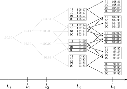
Figure 5.1: The structure of the binomial CRR tree and of the binomial chain for $N=4,M=3,r=0.05,\sigma=0.03$ and $T=0.02$.

6 Numerical experiments

In this Section we report the results of the numeric experiment. We employ the GPR-GHQ method and we test it against a standard Longstaff-Schwartz (LS) approach in all the three stochastic models. Specifically, we report the results for both the two methods and we compare them against the benchmark values. We also report the results by working with fixed computing time, specifically, $30$ seconds, $1$ minute, and $2$ minutes. Finally, as far as the moving average option is considered, we study two different maturities and time-step configurations, that is $T=0.2$ with $N=50$ and $T=1.0$ with $N=250$, which correspond to 50 or 250 trading days. We also present two benchmarks, which have been computed through an independent forward Monte Carlo approach. Specifically, the benchmark values are the average discounted payoff values determined according to the optimal exercise strategy based on the continuation value given by GPR-GHQ and by LS respectively. The parameters used to compute the benchmarks are $deg=2$, $P=10^{7}$ for LS, and $Q=64$, $P=8000$ for GPR-GHQ. The number of Monte Carlo paths for the forward step has been determined so that the radius of the $95$ confidence intervals is $0.01.$ For all prices obtained through Monte Carlo procedures, we also report the margins of error at the $95\%$ confidence level.

Numerical procedures have been implemented in MATLAB. The timed comparisons were carried out on a personal computer equipped with an Intel i5-1035G1 processor and 8 GB of RAM, and only one core was used in order to stabilize the calculation times as much as possible. In all other cases, the numerical values were calculated using an 8-core Intel Xeon Gold 6230 20C processor server with 16 GB RAM.

6.1 The Black-Scholes model

The parameters for the Black-Scholes model are the same used by Bernhart et al., [5] (see Table (1)).

Tables (2), (3) and (4) report the results for LS, GPR-GHQ, and BC for different values of $M$, by changing the numerical parameters of the methods. Specifically, (2) is referred to $T=0.2$, while Table (4) is referred to $T=1.0$. Moreover, Table (2) also reports the results obtained by Bernhart et al., [5] and Lelong, [22]. Finally, Table (5) reports the results of the test with fixed computational time. In this particular case, we exclude the BC method from the comparison, as it does not allow to select the discretization parameters in order to obtain a predetermined computational time.

Looking at values in Table (2), we can observe that the results obtained with the three methods are substantially consistent with each other and with the values in the literature. For small values of $M$ (say $M\leq 10$), LS and GPR-GHQ give very similar values, while BC underestimates the exact value. For $M=20$, the three methods return essentially the same price, however, BC should be preferred as it stands out for its calculation speed, less than one second. Also for $M=30$ the three methods provide similar prices, but the results obtained through BC and GPR-GHQ are slightly higher than those of LS, which indicates that LS loses effectiveness in case of large size. This trend is confirmed by the comparison between the GPR-GHQ and LS benchmarks: the continuation value provided by GPR-GHQ is more accurate than that provided by LS, thus obtaining a better exercise strategy. Note that the ability to approximate the continuation value of LS for large values of $M$ is limited by the use of a polynomial of small degree, a limitation imposed by the large size of the problem. The results presented in Table (4) have similar properties to those of Table (2), however, we observe that BC loses accuracy in this case.

Finally, by examining Table (5), we observe that, given the same time, GPR-GHQ computation is often more efficient than LS. This difference is particularly evident for $M=20$ and $M=30$, as LS suffers from overfitting which is due to the small number of random trajectories considered by the algorithm, in order to reach the fixed computational time.

Symbol	Meaning	Value
$S_{0}$	Initial spot value	$100$
$r$	Risk free i.r.	$0.05$
$\sigma$	Volatility	$0.3$
$T$	Maturity	$0.2$ or $1.0$

Table 1: Parameters employed for the numerical experiments in the Black-Scholes model.

Longstaff-Schwartz

Benchmarks

Berhart

Lelong

$deg$

$1$

$2$

GPR-

LS

et al.

$M$

$P$

$10^{4}$

$10^{5}$

$10^{6}$

$10^{4}$

$10^{5}$

$10^{6}$

GHQ

$\phantom{1}2$

$\underset{\left(1\right)}{1.87\pm 0.02}$

$\underset{\left(1\right)}{1.88\pm 0.00}$

$\underset{\left(5\right)}{1.87\pm 0.00}$

$\underset{\left(0\right)}{1.89\pm 0.02}$

$\underset{\left(1\right)}{1.87\pm 0.00}$

$\underset{\left(5\right)}{1.88\pm 0.00}$

$\underset{\pm 0.01}{1.90}$

$\underset{\pm 0.01}{1.89}$

$1.890$

$\phantom{1}3$

$\underset{\left(1\right)}{2.69\pm 0.02}$

$\underset{\left(2\right)}{2.69\pm 0.01}$

$\underset{\left(10\right)}{2.69\pm 0.00}$

$\underset{\left(0\right)}{2.70\pm 0.02}$

$\underset{\left(2\right)}{2.69\pm 0.01}$

$\underset{\left(14\right)}{2.69\pm 0.00}$

$\underset{\pm 0.01}{2.68}$

$\underset{\pm 0.01}{2.69}$

$2.684$

$\phantom{1}4$

$\underset{\left(1\right)}{3.20\pm 0.03}$

$\underset{\left(2\right)}{3.19\pm 0.01}$

$\underset{\left(12\right)}{3.19\pm 0.00}$

$\underset{\left(0\right)}{3.20\pm 0.03}$

$\underset{\left(3\right)}{3.20\pm 0.01}$

$\underset{\left(25\right)}{3.19\pm 0.00}$

$\underset{\pm 0.01}{3.19}$

$\underset{\pm 0.01}{3.19}$

$3.183$

$\phantom{1}5$

$\underset{\left(1\right)}{3.55\pm 0.04}$

$\underset{\left(2\right)}{3.54\pm 0.01}$

$\underset{\left(12\right)}{3.54\pm 0.00}$

$\underset{\left(1\right)}{3.55\pm 0.04}$

$\underset{\left(4\right)}{3.55\pm 0.01}$

$\underset{\left(31\right)}{3.54\pm 0.00}$

$\underset{\pm 0.01}{3.54}$

$\underset{\pm 0.01}{3.54}$

$3.526$

$3.531$

$\phantom{1}6$

$\underset{\left(1\right)}{3.79\pm 0.04}$

$\underset{\left(3\right)}{3.79\pm 0.01}$

$\underset{\left(14\right)}{3.79\pm 0.00}$

$\underset{\left(1\right)}{3.82\pm 0.04}$

$\underset{\left(5\right)}{3.80\pm 0.01}$

$\underset{\left(49\right)}{3.79\pm 0.00}$

$\underset{\pm 0.01}{3.80}$

$\underset{\pm 0.01}{3.79}$

$3.773$

$\phantom{1}7$

$\underset{\left(1\right)}{3.98\pm 0.05}$

$\underset{\left(3\right)}{3.98\pm 0.02}$

$\underset{\left(15\right)}{3.98\pm 0.00}$

$\underset{\left(1\right)}{4.00\pm 0.05}$

$\underset{\left(6\right)}{3.99\pm 0.01}$

$\underset{\left(52\right)}{3.99\pm 0.00}$

$\underset{\pm 0.01}{3.99}$

$\underset{\pm 0.01}{3.99}$

$3.955$

$\phantom{1}8$

$\underset{\left(1\right)}{4.14\pm 0.05}$

$\underset{\left(3\right)}{4.12\pm 0.02}$

$\underset{\left(18\right)}{4.12\pm 0.01}$

$\underset{\left(2\right)}{4.15\pm 0.05}$

$\underset{\left(8\right)}{4.14\pm 0.02}$

$\underset{\left(76\right)}{4.13\pm 0.01}$

$\underset{\pm 0.01}{4.13}$

$\underset{\pm 0.01}{4.13}$

$4.092$

$\text{$\phantom{1}$}9$

$\underset{\left(1\right)}{4.24\pm 0.06}$

$\underset{\left(3\right)}{4.23\pm 0.02}$

$\underset{\left(22\right)}{4.22\pm 0.01}$

$\underset{\left(2\right)}{4.26\pm 0.05}$

$\underset{\left(11\right)}{4.25\pm 0.02}$

$\underset{\left(94\right)}{4.24\pm 0.01}$

$\underset{\pm 0.01}{4.25}$

$\underset{\pm 0.01}{4.24}$

$4.193$

$10$

$\underset{\left(1\right)}{4.32\pm 0.06}$

$\underset{\left(5\right)}{4.31\pm 0.02}$

$\underset{\left(22\right)}{4.30\pm 0.01}$

$\underset{\left(3\right)}{4.36\pm 0.06}$

$\underset{\left(12\right)}{4.33\pm 0.02}$

$\underset{\left(122\right)}{4.33\pm 0.01}$

$\underset{\pm 0.01}{4.33}$

$\underset{\pm 0.01}{4.33}$

$4.268$

$4.302$

$20$

$\underset{\left(2\right)}{4.40\pm 0.10}$

$\underset{\left(7\right)}{4.41\pm 0.03}$

$\underset{\left(59\right)}{4.39\pm 0.01}$

$\underset{\left(12\right)}{4.61\pm 0.09}$

$\underset{\left(53\right)}{4.49\pm 0.03}$

$\underset{\left(492\right)}{4.47\pm 0.01}$

$\underset{\pm 0.01}{4.48}$

$\underset{\pm 0.01}{4.47}$

$30$

$\underset{\left(2\right)}{4.07\pm 0.11}$

$\underset{\left(9\right)}{4.06\pm 0.04}$

$\underset{\left(65\right)}{4.05\pm 0.01}$

$\underset{\left(24\right)}{4.40\pm 0.11}$

$\underset{\left(105\right)}{4.18\pm 0.03}$

$\underset{\left(929\right)}{4.13\pm 0.01}$

$\underset{\pm 0.01}{4.16}$

$\underset{\pm 0.01}{4.14}$

		GPR-GHQ														Benchmarks		Berhart	Lelong
	$Q$	$8$				$16$				$32$				$64$		GPR-	LS	et al.
$M$	$P$	$250$	$1000$	$4000$		$250$	$1000$	$4000$		$250$	$1000$	$4000$		$8000$		GHQ
$\phantom{1}2$		$\underset{\left(2\right)}{1.812}$				$\underset{\left(2\right)}{1.873}$				$\underset{\left(4\right)}{1.882}$				$\underset{\left(8\right)}{1.891}$		$\underset{\pm 0.01}{1.90}$	$\underset{\pm 0.01}{1.89}$	$1.890$
$\phantom{1}3$		$\underset{\left(19\right)}{2.676}$	$\underset{\left(109\right)}{2.680}$	$\underset{\left(515\right)}{2.682}$		$\underset{\left(18\right)}{2.680}$	$\underset{\left(116\right)}{2.683}$	$\underset{\left(549\right)}{2.684}$		$\underset{\left(18\right)}{2.683}$	$\underset{\left(136\right)}{2.685}$	$\underset{\left(581\right)}{2.685}$		$\underset{\left(1297\right)}{2.687}$		$\underset{\pm 0.01}{2.68}$	$\underset{\pm 0.01}{2.69}$	$2.684$
$\phantom{1}4$		$\underset{\left(12\right)}{3.184}$	$\underset{\left(125\right)}{3.185}$	$\underset{\left(430\right)}{3.190}$		$\underset{\left(15\right)}{3.186}$	$\underset{\left(128\right)}{3.185}$	$\underset{\left(480\right)}{3.188}$		$\underset{\left(18\right)}{3.190}$	$\underset{\left(99\right)}{3.185}$	$\underset{\left(693\right)}{3.189}$		$\underset{\left(1334\right)}{3.190}$		$\underset{\pm 0.01}{3.19}$	$\underset{\pm 0.01}{3.19}$	$3.183$
$\phantom{1}5$		$\underset{\left(19\right)}{3.531}$	$\underset{\left(98\right)}{3.535}$	$\underset{\left(394\right)}{3.539}$		$\underset{\left(19\right)}{3.536}$	$\underset{\left(107\right)}{3.535}$	$\underset{\left(408\right)}{3.539}$		$\underset{\left(20\right)}{3.539}$	$\underset{\left(103\right)}{3.535}$	$\underset{\left(460\right)}{3.540}$		$\underset{\left(1504\right)}{3.540}$		$\underset{\pm 0.01}{3.54}$	$\underset{\pm 0.01}{3.54}$	$3.526$	$3.531$
$\phantom{1}6$		$\underset{\left(11\right)}{3.784}$	$\underset{\left(72\right)}{3.786}$	$\underset{\left(361\right)}{3.790}$		$\underset{\left(11\right)}{3.791}$	$\underset{\left(77\right)}{3.790}$	$\underset{\left(333\right)}{3.792}$		$\underset{\left(14\right)}{3.793}$	$\underset{\left(84\right)}{3.795}$	$\underset{\left(551\right)}{3.795}$		$\underset{\left(1402\right)}{3.795}$		$\underset{\pm 0.01}{3.80}$	$\underset{\pm 0.01}{3.79}$	$3.773$
$\phantom{1}7$		$\underset{\left(12\right)}{3.976}$	$\underset{\left(93\right)}{3.977}$	$\underset{\left(408\right)}{3.980}$		$\underset{\left(12\right)}{3.981}$	$\underset{\left(85\right)}{3.985}$	$\underset{\left(359\right)}{3.986}$		$\underset{\left(24\right)}{3.983}$	$\underset{\left(114\right)}{3.986}$	$\underset{\left(459\right)}{3.986}$		$\underset{\left(1523\right)}{3.987}$		$\underset{\pm 0.01}{3.99}$	$\underset{\pm 0.01}{3.99}$	$3.955$
$\phantom{1}8$		$\underset{\left(13\right)}{4.121}$	$\underset{\left(74\right)}{4.128}$	$\underset{\left(345\right)}{4.126}$		$\underset{\left(11\right)}{4.125}$	$\underset{\left(81\right)}{4.130}$	$\underset{\left(335\right)}{4.132}$		$\underset{\left(13\right)}{4.126}$	$\underset{\left(79\right)}{4.130}$	$\underset{\left(507\right)}{4.132}$		$\underset{\left(1214\right)}{4.132}$		$\underset{\pm 0.01}{4.13}$	$\underset{\pm 0.01}{4.13}$	$4.092$
$\text{$\phantom{1}$}9$		$\underset{\left(12\right)}{4.233}$	$\underset{\left(74\right)}{4.239}$	$\underset{\left(346\right)}{4.241}$		$\underset{\left(13\right)}{4.235}$	$\underset{\left(72\right)}{4.241}$	$\underset{\left(369\right)}{4.242}$		$\underset{\left(19\right)}{4.236}$	$\underset{\left(91\right)}{4.240}$	$\underset{\left(351\right)}{4.243}$		$\underset{\left(1143\right)}{4.243}$		$\underset{\pm 0.01}{4.25}$	$\underset{\pm 0.01}{4.24}$	$4.193$
$10$		$\underset{\left(11\right)}{4.319}$	$\underset{\left(69\right)}{4.325}$	$\underset{\left(337\right)}{4.328}$		$\underset{\left(14\right)}{4.318}$	$\underset{\left(64\right)}{4.325}$	$\underset{\left(343\right)}{4.328}$		$\underset{\left(12\right)}{4.319}$	$\underset{\left(79\right)}{4.325}$	$\underset{\left(349\right)}{4.328}$		$\underset{\left(1186\right)}{4.328}$		$\underset{\pm 0.01}{4.34}$	$\underset{\pm 0.01}{4.33}$	$4.268$	$4.302$
$20$		$\underset{\left(26\right)}{4.473}$	$\underset{\left(84\right)}{4.469}$	$\underset{\left(239\right)}{4.475}$		$\underset{\left(28\right)}{4.473}$	$\underset{\left(63\right)}{4.469}$	$\underset{\left(308\right)}{4.475}$		$\underset{\left(30\right)}{4.472}$	$\underset{\left(68\right)}{4.468}$	$\underset{\left(303\right)}{4.475}$		$\underset{\left(959\right)}{4.476}$		$\underset{\pm 0.01}{4.48}$	$\underset{\pm 0.01}{4.47}$
$30$		$\underset{\left(13\right)}{4.142}$	$\underset{\left(63\right)}{4.141}$	$\underset{\left(204\right)}{4.143}$		$\underset{\left(12\right)}{4.142}$	$\underset{\left(47\right)}{4.141}$	$\underset{\left(184\right)}{4.143}$		$\underset{\left(12\right)}{4.142}$	$\underset{\left(51\right)}{4.141}$	$\underset{\left(202\right)}{4.143}$		$\underset{\left(586\right)}{4.144}$		$\underset{\pm 0.01}{4.16}$	$\underset{\pm 0.01}{4.14}$

Table 2: Black-Scholes model with $T=0.2$ and $N=50$ time steps. Values in brackets are the computational times measured in seconds.

		BC		Benchmarks		Berhart	Lelong
$M$				GPR-GHQ	LS	et al.
$\phantom{1}2$		$\underset{\left(1\cdot 10^{-2}\right)}{0.94}$		$\underset{\pm 0.01}{1.90}$	$\underset{\pm 0.01}{1.89}$	$1.890$
$\phantom{1}3$		$\underset{\left(1\cdot 10^{-2}\right)}{1.87}$		$\underset{\pm 0.01}{2.68}$	$\underset{\pm 0.01}{2.69}$	$2.684$
$\phantom{1}4$		$\underset{\left(1\cdot 10^{-2}\right)}{2.75}$		$\underset{\pm 0.01}{3.19}$	$\underset{\pm 0.01}{3.19}$	$3.183$
$\phantom{1}5$		$\underset{\left(1\cdot 10^{-2}\right)}{3.32}$		$\underset{\pm 0.01}{3.54}$	$\underset{\pm 0.01}{3.54}$	$3.526$	$3.531$
$\phantom{1}6$		$\underset{\left(1\cdot 10^{-2}\right)}{3.60}$		$\underset{\pm 0.01}{3.80}$	$\underset{\pm 0.01}{3.79}$	$3.773$
$\phantom{1}7$		$\underset{\left(2\cdot 10^{-2}\right)}{3.86}$		$\underset{\pm 0.01}{3.99}$	$\underset{\pm 0.01}{3.99}$	$3.955$
$\phantom{1}8$		$\underset{\left(1\cdot 10^{-2}\right)}{4.04}$		$\underset{\pm 0.01}{4.13}$	$\underset{\pm 0.01}{4.13}$	$4.092$
$\text{$\phantom{1}$}9$		$\underset{\left(1\cdot 10^{-2}\right)}{4.17}$		$\underset{\pm 0.01}{4.25}$	$\underset{\pm 0.01}{4.24}$	$4.193$
$10$		$\underset{\left(2\cdot 10^{-2}\right)}{4.28}$		$\underset{\pm 0.01}{4.34}$	$\underset{\pm 0.01}{4.33}$	$4.268$	$4.302$
$20$		$\underset{\left(3\cdot 10^{-1}\right)}{4.49}$		$\underset{\pm 0.01}{4.48}$	$\underset{\pm 0.01}{4.47}$
$30$		$\underset{\left(308\right)}{4.16}$		$\underset{\pm 0.01}{4.16}$	$\underset{\pm 0.01}{4.14}$

Table 3: Black-Scholes model with $T=0.2$ and $N=50$ time steps. Values in brackets are the computational times measured in seconds.

		Longstaff-Schwartz								Benchmarks
	$deg$	$1$				$2$				GPR-	LS
$M$	$P$	$10^{4}$	$10^{5}$	$10^{6}$		$10^{4}$	$10^{5}$	$10^{6}$		GHQ
$\phantom{1}2$		$\underset{\left(1\right)}{2.29\pm 0.02}$	$\underset{\left(3\right)}{2.30\pm 0.01}$	$\underset{\left(26\right)}{2.30\pm 0.00}$		$\underset{\left(0\right)}{2.31\pm 0.02}$	$\underset{\left(2\right)}{2.30\pm 0.01}$	$\underset{\left(25\right)}{2.30\pm 0.00}$		$\underset{\pm 0.01}{2.44}$	$\underset{\pm 0.01}{2.44}$
$10$		$\underset{\left(4\right)}{6.90\pm 0.06}$	$\underset{\left(18\right)}{6.89\pm 0.02}$	$\underset{\left(163\right)}{6.88\pm 0.01}$		$\underset{\left(15\right)}{6.93\pm 0.06}$	$\underset{\left(72\right)}{6.90\pm 0.02}$	$\underset{\left(750\right)}{6.90\pm 0.01}$		$\underset{\pm 0.01}{6.90}$	$\underset{\pm 0.01}{6.90}$
$20$		$\underset{\left(9\right)}{8.67\pm 0.09}$	$\underset{\left(42\right)}{8.65\pm 0.03}$	$\underset{\left(423\right)}{8.64\pm 0.01}$		$\underset{\left(90\right)}{8.77\pm 0.10}$	$\underset{\left(410\right)}{8.69\pm 0.03}$	$\underset{\left(3634\right)}{8.66\pm 0.01}$		$\underset{\pm 0.01}{8.68}$	$\underset{\pm 0.01}{8.67}$
$30$		$\underset{\left(17\right)}{9.53\pm 0.12}$	$\underset{\left(79\right)}{9.52\pm 0.04}$	$\underset{\left(794\right)}{9.50\pm 0.01}$		$\underset{\left(259\right)}{9.75\pm 0.13}$	$\underset{\left(1230\right)}{9.60\pm 0.04}$	$\underset{\left(11939\right)}{9.55\pm 0.01}$		$\underset{\pm 0.01}{9.57}$	$\underset{\pm 0.01}{9.54}$

		GPR-GHQ														Benchmarks
	$G$	$8$				$16$				$32$				$64$		GPR-	LS
$M$	$P$	$250$	$1000$	$4000$		$250$	$1000$	$4000$		$250$	$1000$	$4000$		$8000$		GHQ
$\phantom{1}2$		$\underset{\left(2\right)}{2.504}$				$\underset{\left(4\right)}{2.466}$				$\underset{\left(4\right)}{2.427}$				$\underset{\left(18\right)}{2.436}$		$\underset{\pm 0.01}{2.44}$	$\underset{\pm 0.01}{2.44}$
$10$		$\underset{\left(55\right)}{6.891}$	$\underset{\left(585\right)}{6.888}$	$\underset{\left(3404\right)}{6.896}$		$\underset{\left(59\right)}{6.888}$	$\underset{\left(434\right)}{6.894}$	$\underset{\left(2038\right)}{6.901}$		$\underset{\left(64\right)}{6.889}$	$\underset{\left(572\right)}{6.896}$	$\underset{\left(2360\right)}{6.901}$		$\underset{\left(10893\right)}{6.903}$		$\underset{\pm 0.01}{6.90}$	$\underset{\pm 0.01}{6.90}$
$20$		$\underset{\left(72\right)}{8.651}$	$\underset{\left(596\right)}{8.656}$	$\underset{\left(2340\right)}{8.668}$		$\underset{\left(73\right)}{8.650}$	$\underset{\left(768\right)}{8.657}$	$\underset{\left(2761\right)}{8.669}$		$\underset{\left(77\right)}{8.647}$	$\underset{\left(652\right)}{8.656}$	$\underset{\left(3150\right)}{8.670}$		$\underset{\left(7558\right)}{8.673}$		$\underset{\pm 0.01}{8.68}$	$\underset{\pm 0.01}{8.67}$
$30$		$\underset{\left(57\right)}{9.512}$	$\underset{\left(618\right)}{9.531}$	$\underset{\left(2594\right)}{9.548}$		$\underset{\left(74\right)}{9.511}$	$\underset{\left(600\right)}{9.533}$	$\underset{\left(2680\right)}{9.549}$		$\underset{\left(76\right)}{9.511}$	$\underset{\left(634\right)}{9.532}$	$\underset{\left(3086\right)}{9.549}$		$\underset{\left(7526\right)}{9.554}$		$\underset{\pm 0.01}{9.57}$	$\underset{\pm 0.01}{9.54}$

		BC method		Benchmarks
$M$				GPR-GHQ	LS
$\phantom{1}2$		$\underset{\left(1\cdot 10^{-2}\right)}{0.94}$		$\underset{\pm 0.01}{2.44}$	$\underset{\pm 0.01}{2.44}$
$10$		$\underset{\left(2\cdot 10^{-2}\right)}{6.43}$		$\underset{\pm 0.01}{6.90}$	$\underset{\pm 0.01}{6.90}$
$20$		$\underset{\left(2\right)}{8.49}$		$\underset{\pm 0.01}{8.68}$	$\underset{\pm 0.01}{8.67}$
$30$		$\underset{\left(1598\right)}{9.47}$		$\underset{\pm 0.01}{9.57}$	$\underset{\pm 0.01}{9.54}$

Table 4: Black-Scholes model with $T=1.0$ and $N=250$ time steps. Values in brackets are the computational times measured in seconds.

Comparison
				Benchmarks
$M$	LS	GPR-GHQ		GPR-	LS
	$30\ \text{s}$			GHQ
$\phantom{1}2$	$\underset{\left(1.0e6;4\right)}{1.88\pm 0.00}$	$\underset{\left(1;1024\right)}{1.89^{*}}$		$\underset{\pm 0.01}{1.89}$	$\underset{\pm 0.01}{1.89}$
$10$	$\underset{\left(1.0e5;2\right)}{4.33^{*}\pm 0.02}$	$\underset{\left(500;8\right)}{4.32}$		$\underset{\pm 0.01}{4.34}$	$\underset{\pm 0.01}{4.33}$
$20$	$\underset{\left(2.0e4;2\right)}{4.57\pm 0.06}$	$\underset{\left(550;4\right)}{4.47^{*}}$		$\underset{\pm 0.01}{4.48}$	$\underset{\pm 0.01}{4.47}$
$30$	$\underset{\left(1.0e4;2\right)}{4.40\pm 0.11}$	$\underset{\left(650;4\right)}{4.14^{*}}$		$\underset{\pm 0.01}{4.16}$	$\underset{\pm 0.01}{4.14}$
	$1\ \text{min}$
$\phantom{1}2$	$\underset{\left(1.0e6;4\right)}{1.88\pm 0.00}$	$\underset{\left(1;1024\right)}{1.89^{*}}$		$\underset{\pm 0.01}{1.89}$	$\underset{\pm 0.01}{1.89}$
$10$	$\underset{\left(1.5e5;2\right)}{4.33^{*}\pm 0.02}$	$\underset{\left(700;16\right)}{4.32}$		$\underset{\pm 0.01}{4.34}$	$\underset{\pm 0.01}{4.33}$
$20$	$\underset{\left(4.0e4;2\right)}{4.51\pm 0.04}$	$\underset{\left(650;6\right)}{4.47^{*}}$		$\underset{\pm 0.01}{4.48}$	$\underset{\pm 0.01}{4.47}$
$30$	$\underset{\left(2.0e4;2\right)}{4.31\pm 0.08}$	$\underset{\left(750;4\right)}{4.14^{*}}$		$\underset{\pm 0.01}{4.16}$	$\underset{\pm 0.01}{4.14}$
	$2\ \text{min}$
$\phantom{1}2$	$\underset{\left(1.0e6;4\right)}{1.88\pm 0.00}$	$\underset{\left(1;1024\right)}{1.89^{*}}$		$\underset{\pm 0.01}{1.89}$	$\underset{\pm 0.01}{1.89}$
$10$	$\underset{\left(2.7e5;2\right)}{4.33^{*}\pm 0.02}$	$\underset{\left(1500;16\right)}{4.33^{*}}$		$\underset{\pm 0.01}{4.34}$	$\underset{\pm 0.01}{4.33}$
$20$	$\underset{\left(8.1e4;2\right)}{4.49\pm 0.03}$	$\underset{\left(750;8\right)}{4.47^{*}}$		$\underset{\pm 0.01}{4.48}$	$\underset{\pm 0.01}{4.47}$
$30$	$\underset{\left(4.0e4;2\right)}{4.23\pm 0.05}$	$\underset{\left(1100;4\right)}{4.14^{*}}$		$\underset{\pm 0.01}{4.16}$	$\underset{\pm 0.01}{4.14}$

Table 5: Black-Scholes model. Comparison between the Longstaff-Schwartz and the GPR-GHQ methods for $T=0.2$ and $N=50$. Values in brackets are the numerical parameters: number of simulations and polynomial degree for LS, $P$ and $Q$ for the GPR-GHQ method. Each asterisk indicates the best value for a predetermined run-time as the closest to the benchmarks.

6.2 The Clewlow-Strickland model

The parameters for the Clewlow-Strickland model are the same used by Dong and Kang, [14] (see Table (6)). Tables (7) and (8) report the numerical results for different values of $M$ and for different parameter configurations. Note that both numerical methods tend to converge to the same results. Table (9) reports the results for the tests with fixed computational time. The two methods are essentially equivalent for $M\leq 20$ while for $M=30$ GPR-GHQ converges much faster to the correct value as LS over-estimates the price, suffering from overfitting.

Symbol	Meaning	Value
$F\left(0,t\right)$	Initial forward curve	$100$
$r$	Risk free i.r.	$0.05$
$\alpha$	Mean reversion speed	$5$
$\sigma$	Volatility	$0.5$
$T$	Maturity	$0.2$ or $1.0$

Table 6: Parameters employed for the numerical experiments in the Clewlow-Strickland model.

		Longstaff-Schwartz								Benchmarks
	$deg$	$1$				$2$				GPR-	LS
$M$	$P$	$10^{4}$	$10^{5}$	$10^{6}$		$10^{4}$	$10^{5}$	$10^{6}$		GHQ
$\phantom{1}2$		$\underset{\left(1\right)}{3.14\pm 0.02}$	$\underset{\left(2\right)}{3.14\pm 0.01}$	$\underset{\left(9\right)}{3.14\pm 0.00}$		$\underset{\left(1\right)}{3.14\pm 0.02}$	$\underset{\left(1\right)}{3.14\pm 0.01}$	$\underset{\left(10\right)}{3.14\pm 0.00}$		$\underset{\pm 0.01}{3.14}$	$\underset{\pm 0.01}{3.14}$
$10$		$\underset{\left(1\right)}{7.26\pm 0.07}$	$\underset{\left(4\right)}{7.24\pm 0.02}$	$\underset{\left(26\right)}{7.23\pm 0.01}$		$\underset{\left(2\right)}{7.27\pm 0.07}$	$\underset{\left(12\right)}{7.25\pm 0.02}$	$\underset{\left(134\right)}{7.27\pm 0.01}$		$\underset{\pm 0.01}{7.27}$	$\underset{\pm 0.01}{7.27}$
$20$		$\underset{\left(2\right)}{7.25\pm 0.11}$	$\underset{\left(6\right)}{7.26\pm 0.03}$	$\underset{\left(56\right)}{7.24\pm 0.01}$		$\underset{\left(11\right)}{7.54\pm 0.10}$	$\underset{\left(52\right)}{7.36\pm 0.03}$	$\underset{\left(441\right)}{7.37\pm 0.01}$		$\underset{\pm 0.01}{7.37}$	$\underset{\pm 0.01}{7.36}$
$30$		$\underset{\left(2\right)}{6.30\pm 0.12}$	$\underset{\left(8\right)}{6.32\pm 0.04}$	$\underset{\left(61\right)}{6.31\pm 0.01}$		$\underset{\left(24\right)}{6.83\pm 0.12}$	$\underset{\left(104\right)}{6.45\pm 0.04}$	$\underset{\left(1002\right)}{6.43\pm 0.01}$		$\underset{\pm 0.01}{6.43}$	$\underset{\pm 0.01}{6.42}$

	GPR-GHQ															Benchmarks
	$G$	$8$				$16$				$32$				$64$		GPR-	LS
$M$	$P$	$250$	$1000$	$4000$		$250$	$1000$	$4000$		$250$	$1000$	$4000$		$8000$		GHQ
$\phantom{1}2$		$\underset{\left(32\right)}{3.003}$	$\underset{\left(109\right)}{3.003}$	$\underset{\left(443\right)}{3.003}$		$\underset{\left(34\right)}{3.109}$	$\underset{\left(94\right)}{3.109}$	$\underset{\left(391\right)}{3.109}$		$\underset{\left(32\right)}{3.124}$	$\underset{\left(116\right)}{3.124}$	$\underset{\left(430\right)}{3.124}$		$\underset{\left(1253\right)}{3.140}$		$\underset{\pm 0.01}{3.14}$	$\underset{\pm 0.01}{3.14}$
$10$		$\underset{\left(11\right)}{7.305}$	$\underset{\left(59\right)}{7.281}$	$\underset{\left(362\right)}{7.275}$		$\underset{\left(11\right)}{7.296}$	$\underset{\left(65\right)}{7.278}$	$\underset{\left(269\right)}{7.273}$		$\underset{\left(13\right)}{7.299}$	$\underset{\left(75\right)}{7.274}$	$\underset{\left(358\right)}{7.272}$		$\underset{\left(1164\right)}{7.273}$		$\underset{\pm 0.01}{7.27}$	$\underset{\pm 0.01}{7.27}$
$20$		$\underset{\left(9\right)}{7.414}$	$\underset{\left(53\right)}{7.384}$	$\underset{\left(203\right)}{7.378}$		$\underset{\left(10\right)}{7.411}$	$\underset{\left(55\right)}{7.382}$	$\underset{\left(220\right)}{7.377}$		$\underset{\left(11\right)}{7.409}$	$\underset{\left(63\right)}{7.381}$	$\underset{\left(491\right)}{7.377}$		$\underset{\left(956\right)}{7.376}$		$\underset{\pm 0.01}{7.37}$	$\underset{\pm 0.01}{7.36}$
$30$		$\underset{\left(9\right)}{6.427}$	$\underset{\left(38\right)}{6.432}$	$\underset{\left(142\right)}{6.437}$		$\underset{\left(8\right)}{6.426}$	$\underset{\left(43\right)}{6.431}$	$\underset{\left(247\right)}{6.437}$		$\underset{\left(9\right)}{6.426}$	$\underset{\left(48\right)}{6.431}$	$\underset{\left(260\right)}{6.437}$		$\underset{\left(687\right)}{6.437}$		$\underset{\pm 0.01}{6.43}$	$\underset{\pm 0.01}{6.42}$

Table 7: Clewlow-Strickland model with $T=0.2$ and $N=50$ time steps. Values in brackets are the computational times measured in seconds.

		Longstaff-Schwartz								Benchmarks
	$deg$	$1$				$2$				GPR-	LS
$M$	$P$	$10^{4}$	$10^{5}$	$10^{6}$		$10^{4}$	$10^{5}$	$10^{6}$		GHQ
$\phantom{1}2$		$\underset{\left(3\right)}{4.10\pm 0.02}$	$\underset{\left(6\right)}{4.11\pm 0.01}$	$\underset{\left(41\right)}{4.11\pm 0.00}$		$\underset{\left(1\right)}{4.11\pm 0.02}$	$\underset{\left(7\right)}{4.11\pm 0.01}$	$\underset{\left(53\right)}{4.11\pm 0.00}$		$\underset{\pm 0.01}{4.12}$	$\underset{\pm 0.01}{4.11}$
$10$		$\underset{\left(4\right)}{11.73\pm 0.06}$	$\underset{\left(17\right)}{11.75\pm 0.02}$	$\underset{\left(160\right)}{11.73\pm 0.01}$		$\underset{\left(15\right)}{11.80\pm 0.06}$	$\underset{\left(71\right)}{11.76\pm 0.02}$	$\underset{\left(797\right)}{11.75\pm 0.01}$		$\underset{\pm 0.01}{11.76}$	$\underset{\pm 0.01}{11.75}$
$20$		$\underset{\left(10\right)}{14.75\pm 0.09}$	$\underset{\left(41\right)}{14.77\pm 0.03}$	$\underset{\left(437\right)}{14.75\pm 0.01}$		$\underset{\left(87\right)}{15.12\pm 0.09}$	$\underset{\left(405\right)}{14.83\pm 0.03}$	$\underset{\left(3531\right)}{14.80\pm 0.01}$		$\underset{\pm 0.01}{14.81}$	$\underset{\pm 0.01}{14.79}$
$30$		$\underset{\left(18\right)}{16.16\pm 0.11}$	$\underset{\left(81\right)}{16.21\pm 0.04}$	$\underset{\left(841\right)}{16.20\pm 0.01}$		$\underset{\left(270\right)}{17.08\pm 0.11}$	$\underset{\left(1183\right)}{16.37\pm 0.03}$	$\underset{\left(11968\right)}{16.28\pm 0.01}$		$\underset{\pm 0.01}{16.30}$	$\underset{\pm 0.01}{16.28}$

		GPR-GHQ														Benchmarks
	$G$	$8$				$16$				$32$				$64$		GPR-	LS
$M$	$P$	$250$	$1000$	$4000$		$250$	$1000$	$4000$		$250$	$1000$	$4000$		$8000$		GHQ
$\phantom{1}2$		$\underset{\left(50\right)}{4.214}$	$\underset{\left(509\right)}{4.214}$	$\underset{\left(1863\right)}{4.214}$		$\underset{\left(61\right)}{4.138}$	$\underset{\left(383\right)}{4.138}$	$\underset{\left(2078\right)}{4.139}$		$\underset{\left(60\right)}{4.106}$	$\underset{\left(433\right)}{4.107}$	$\underset{\left(3016\right)}{4.107}$		$\underset{\left(8759\right)}{4.110}$		$\underset{\pm 0.01}{4.12}$	$\underset{\pm 0.01}{4.11}$
$10$		$\underset{\left(57\right)}{11.777}$	$\underset{\left(401\right)}{11.777}$	$\underset{\left(1696\right)}{11.762}$		$\underset{\left(60\right)}{11.786}$	$\underset{\left(537\right)}{11.772}$	$\underset{\left(1981\right)}{11.760}$		$\underset{\left(69\right)}{11.787}$	$\underset{\left(482\right)}{11.770}$	$\underset{\left(2475\right)}{11.759}$		$\underset{\left(7652\right)}{11.758}$		$\underset{\pm 0.01}{11.76}$	$\underset{\pm 0.01}{11.75}$
$20$		$\underset{\left(86\right)}{15.124}$	$\underset{\left(508\right)}{14.887}$	$\underset{\left(2585\right)}{14.835}$		$\underset{\left(92\right)}{15.125}$	$\underset{\left(637\right)}{14.888}$	$\underset{\left(2065\right)}{14.836}$		$\underset{\left(104\right)}{15.124}$	$\underset{\left(542\right)}{14.887}$	$\underset{\left(3035\right)}{14.836}$		$\underset{\left(7486\right)}{14.826}$		$\underset{\pm 0.01}{14.81}$	$\underset{\pm 0.01}{14.79}$
$30$		$\underset{\left(74\right)}{16.718}$	$\underset{\left(551\right)}{16.408}$	$\underset{\left(1936\right)}{16.333}$		$\underset{\left(76\right)}{16.720}$	$\underset{\left(494\right)}{16.409}$	$\underset{\left(2144\right)}{16.332}$		$\underset{\left(93\right)}{16.721}$	$\underset{\left(558\right)}{16.409}$	$\underset{\left(2235\right)}{16.332}$		$\underset{\left(7067\right)}{16.325}$		$\underset{\pm 0.01}{16.30}$	$\underset{\pm 0.01}{16.28}$

Table 8: Clewlow-Strickland model with $T=1.0$ and $N=250$ time steps. Values in brackets are the computational times measured in seconds.

Comparison
				Benchmarks
$M$	LSB	GPR		GPR-	LS
	$30\ \text{s}$			GHQ
$\phantom{1}2$	$\underset{\left(1.0e6;2\right)}{3.14^{*}\pm 0.00}$	$\underset{\left(450;64\right)}{3.14^{*}}$		$\underset{\pm 0.01}{3.14}$	$\underset{\pm 0.01}{3.14}$
$10$	$\underset{\left(1.0e5;2\right)}{7.28^{*}\pm 0.02}$	$\underset{\left(550;16\right)}{7.28^{*}}$		$\underset{\pm 0.01}{7.27}$	$\underset{\pm 0.01}{7.27}$
$20$	$\underset{\left(2.5e4;2\right)}{7.41\pm 0.06}$	$\underset{\left(600;4\right)}{7.38^{*}}$		$\underset{\pm 0.01}{7.37}$	$\underset{\pm 0.01}{7.36}$
$30$	$\underset{\left(1.0e4;2\right)}{6.88\pm 0.12}$	$\underset{\left(750;4\right)}{6.44^{*}}$		$\underset{\pm 0.01}{6.43}$	$\underset{\pm 0.01}{6.42}$
	$1\ \text{min}$
$\phantom{1}2$	$\underset{\left(1.0e6;2\right)}{3.14^{*}\pm 0.00}$	$\underset{\left(600;64\right)}{3.14^{*}}$		$\underset{\pm 0.01}{3.14}$	$\underset{\pm 0.01}{3.14}$
$10$	$\underset{\left(1.7e5;2\right)}{7.28^{*}\pm 0.02}$	$\underset{\left(800;16\right)}{7.28^{*}}$		$\underset{\pm 0.01}{7.27}$	$\underset{\pm 0.01}{7.27}$
$20$	$\underset{\left(4.8e4;2\right)}{7.43\pm 0.04}$	$\underset{\left(900;6\right)}{7.38^{*}}$		$\underset{\pm 0.01}{7.37}$	$\underset{\pm 0.01}{7.36}$
$30$	$\underset{\left(2.0e4;2\right)}{6.77\pm 0.09}$	$\underset{\left(1000;8\right)}{6.43^{*}}$		$\underset{\pm 0.01}{6.43}$	$\underset{\pm 0.01}{6.42}$
	$2\ \text{min}$
$\phantom{1}2$	$\underset{\left(1.0e6;2\right)}{3.14^{*}\pm 0.00}$	$\underset{\left(900;64\right)}{3.14^{*}}$		$\underset{\pm 0.01}{3.14}$	$\underset{\pm 0.01}{3.14}$
$10$	$\underset{\left(3.0e5;2\right)}{7.27^{*}\pm 0.01}$	$\underset{\left(900;32\right)}{7.28}$		$\underset{\pm 0.01}{7.27}$	$\underset{\pm 0.01}{7.27}$
$20$	$\underset{\left(9.0e4;2\right)}{7.37^{*}\pm 0.03}$	$\underset{\left(1100;6\right)}{7.38}$		$\underset{\pm 0.01}{7.37}$	$\underset{\pm 0.01}{7.36}$
$30$	$\underset{\left(3.9e4;2\right)}{6.55\pm 0.06}$	$\underset{\left(1300;8\right)}{6.43^{*}}$		$\underset{\pm 0.01}{6.43}$	$\underset{\pm 0.01}{6.42}$

Table 9: Clewlow-Strickland model. Comparison between the Longstaff-Schwartz and the GPR-GHQ methods for $T=0.2$ and $N=50$. Values in brackets are the numerical parameters: number of simulations and polynomial degree for LS, $P$ and $Q$ for the GPR-GHQ method. Each asterisk indicates the best value for a predetermined run-time as the closest to the benchmarks.

6.3 The rough-Bergomi model

The parameters for the rough-Bergomi model are the same used by Bayer et al., [4] (see Table (10)). Tables (11) and (12) report the numerical results for different values of $M$ and for different parameter configurations. We observe that, in case, the values provided by LS are generally a few cents lower than the benchmarks, which indicates that convergence is slower in the rough-Bergomi model than in the Black-Scholes and Clewlow-Strickland models. Conversely, the values returned by GPR-GHQ are very close to the benchmark values even using small values for $P$ and $Q$. We then observe that, both for LS and for GPR-GHQ, they tend to grow with increasing $J$. This is consistent with the fact that having more information, it is possible to better learn the continuation value and therefore improve the exercise strategy. Obviously, the increase in computational times is the negative aspect that weighs on the choice of large values for $J$. Please note that the differences between $J=7$ and $J=15$ are of the order of at most 1 cent, therefore we used $J=15$ for the calculation of the benchmark.

Table (13) reports the results for the tests with fixed computational time. GPR-GHQ is very often the best method, in particular for $M=20$ and $M=3$0, as well as when the computational target time is 2 minutes. It should be noted that the calculation of the price of a moving average option in the rough-Bergomi model has a greater dimension than the same problem in the Black-Scholes and Clewlow-Strickland models since volatility history must also be included in the set for predictors. Consequently, GPR-GHQ, is particularly efficient to tackle this type of problem.

Symbol	Meaning	Value
$S_{0}$	Initial spot value	$100$
$r$	Risk free i.r.	$0.05$
$\rho$	correlation	$-0.9$
$\xi_{0}$	Forward variance rate	$0.09$
$\eta$	Vol of vol	$1.9$
$T$	Maturity	$0.2$ or $1.0$

Table 10: Parameters employed for the numerical experiments in the Clewlow-Strickland model.

		Longstaff-Schwartz
	$deg$	$1$				$2$				Benchmarks
	$P$	$10^{5}$				$10^{6}$				GPR-	LS
$M$	$J$	$3$	$7$	$15$		$3$	$7$	$15$		GHQ
$\phantom{1}2$		$\underset{\left(4\right)}{2.13\pm 0.01}$	$\underset{\left(6\right)}{2.14\pm 0.01}$	$\underset{\left(17\right)}{2.14\pm 0.01}$		$\underset{\left(94\right)}{2.14\pm 0.00}$	$\underset{\left(477\right)}{2.14\pm 0.00}$	$\underset{\left(2500\right)}{2.15\pm 0.00}$		$\underset{\pm 0.01}{2.17}$	$\underset{\pm 0.01}{2.16}$
$10$		$\underset{\left(5\right)}{3.42\pm 0.02}$	$\underset{\left(8\right)}{3.44\pm 0.02}$	$\underset{\left(16\right)}{3.44\pm 0.02}$		$\underset{\left(346\right)}{3.49\pm 0.00}$	$\underset{\left(561\right)}{3.50\pm 0.00}$	$\underset{\left(3154\right)}{3.50\pm 0.00}$		$\underset{\pm 0.01}{3.57}$	$\underset{\pm 0.01}{3.56}$
$20$		$\underset{\left(9\right)}{3.51\pm 0.02}$	$\underset{\left(11\right)}{3.53\pm 0.02}$	$\underset{\left(16\right)}{3.54\pm 0.02}$		$\underset{\left(861\right)}{3.59\pm 0.01}$	$\underset{\left(1773\right)}{3.60\pm 0.01}$	$\underset{\left(2880\right)}{3.61\pm 0.01}$		$\underset{\pm 0.01}{3.67}$	$\underset{\pm 0.01}{3.65}$
$30$		$\underset{\left(16\right)}{3.32\pm 0.02}$	$\underset{\left(12\right)}{3.34\pm 0.02}$	$\underset{\left(17\right)}{3.35\pm 0.02}$		$\underset{\left(1958\right)}{3.39\pm 0.01}$	$\underset{\left(2200\right)}{3.40\pm 0.01}$	$\underset{\left(4833\right)}{3.41\pm 0.01}$		$\underset{\pm 0.01}{3.44}$	$\underset{\pm 0.01}{3.42}$

		GPR-GHQ
	$G$	$8$								$16$								Benchmarks
	$P$	$4000$				$8000$				$4000$				$8000$				GPR-	LS
$M$	$J$	$3$	$7$	$15$		$3$	$7$	$15$		$3$	$7$	$15$		$3$	$7$	$15$		GHQ
$\phantom{1}2$		$\underset{\left(548\right)}{2.168}$	$\underset{\left(602\right)}{2.161}$	$\underset{\left(608\right)}{2.161}$		$\underset{\left(1355\right)}{2.171}$	$\underset{\left(1408\right)}{2.161}$	$\underset{\left(1440\right)}{2.162}$		$\underset{\left(1058\right)}{2.182}$	$\underset{\left(1135\right)}{2.163}$	$\underset{\left(1150\right)}{2.162}$		$\underset{\left(4630\right)}{2.175}$	$\underset{\left(3056\right)}{2.164}$	$\underset{\left(3203\right)}{2.163}$		$\underset{\pm 0.01}{2.17}$	$\underset{\pm 0.01}{2.16}$
$10$		$\underset{\left(447\right)}{3.545}$	$\underset{\left(472\right)}{3.546}$	$\underset{\left(512\right)}{3.549}$		$\underset{\left(1134\right)}{3.546}$	$\underset{\left(1168\right)}{3.546}$	$\underset{\left(1217\right)}{3.548}$		$\underset{\left(943\right)}{3.544}$	$\underset{\left(987\right)}{3.545}$	$\underset{\left(1028\right)}{3.548}$		$\underset{\left(2713\right)}{3.546}$	$\underset{\left(2890\right)}{3.546}$	$\underset{\left(2768\right)}{3.547}$		$\underset{\pm 0.01}{3.57}$	$\underset{\pm 0.01}{3.56}$
$20$		$\underset{\left(358\right)}{3.666}$	$\underset{\left(349\right)}{3.667}$	$\underset{\left(383\right)}{3.669}$		$\underset{\left(882\right)}{3.661}$	$\underset{\left(880\right)}{3.662}$	$\underset{\left(915\right)}{3.663}$		$\underset{\left(727\right)}{3.666}$	$\underset{\left(1119\right)}{3.667}$	$\underset{\left(738\right)}{3.669}$		$\underset{\left(2083\right)}{3.662}$	$\underset{\left(2062\right)}{3.662}$	$\underset{\left(2118\right)}{3.663}$		$\underset{\pm 0.01}{3.67}$	$\underset{\pm 0.01}{3.65}$
$30$		$\underset{\left(254\right)}{3.462}$	$\underset{\left(269\right)}{3.463}$	$\underset{\left(268\right)}{3.464}$		$\underset{\left(602\right)}{3.454}$	$\underset{\left(625\right)}{3.455}$	$\underset{\left(618\right)}{3.456}$		$\underset{\left(499\right)}{3.463}$	$\underset{\left(518\right)}{3.464}$	$\underset{\left(527\right)}{3.464}$		$\underset{\left(1369\right)}{3.454}$	$\underset{\left(1442\right)}{3.455}$	$\underset{\left(1401\right)}{3.456}$		$\underset{\pm 0.01}{3.44}$	$\underset{\pm 0.01}{3.42}$

Table 11: rough-Bergomi model with $T=0.2$ and $N=50$ time steps. Values in brackets are the computational times measured in seconds.

		Longstaff-Schwartz
	$deg$	$1$				$2$				Benchmarks
	$P$	$10^{5}$				$10^{6}$				GPR-	LS
$M$	$J$	$3$	$7$	$15$		$3$	$7$	$15$		GHQ
$\phantom{1}2$		$\underset{\left(14\right)}{3.16\pm 0.01}$	$\underset{\left(42\right)}{3.16\pm 0.01}$	$\underset{\left(93\right)}{3.17\pm 0.01}$		$\underset{\left(511\right)}{3.16\pm 0.00}$	$\underset{\left(2135\right)}{3.19\pm 0.00}$	$\underset{\left(14111\right)}{3.21\pm 0.00}$		$\underset{\pm 0.01}{3.27}$	$\underset{\pm 0.01}{3.28}$
$10$		$\underset{\left(28\right)}{5.07\pm 0.02}$	$\underset{\left(54\right)}{5.09\pm 0.02}$	$\underset{\left(100\right)}{5.10\pm 0.02}$		$\underset{\left(1732\right)}{5.21\pm 0.01}$	$\underset{\left(2983\right)}{5.24\pm 0.01}$	$\underset{\left(15337\right)}{5.28\pm 0.01}$		$\underset{\pm 0.01}{5.42}$	$\underset{\pm 0.01}{5.42}$
$20$		$\underset{\left(65\right)}{5.80\pm 0.02}$	$\underset{\left(85\right)}{5.84\pm 0.02}$	$\underset{\left(150\right)}{5.87\pm 0.02}$		$\underset{\left(6793\right)}{6.00\pm 0.01}$	$\underset{\left(10188\right)}{6.04\pm 0.01}$	$\underset{\left(19686\right)}{6.07\pm 0.01}$		$\underset{\pm 0.01}{6.25}$	$\underset{\pm 0.01}{6.23}$
$30$		$\underset{\left(105\right)}{6.29\pm 0.02}$	$\underset{\left(126\right)}{6.35\pm 0.02}$	$\underset{\left(225\right)}{6.39\pm 0.02}$		$\underset{\left(17373\right)}{6.53\pm 0.01}$	$\underset{\left(27503\right)}{6.57\pm 0.01}$	$\underset{\left(43294\right)}{6.61\pm 0.01}$		$\underset{\pm 0.01}{6.79}$	$\underset{\pm 0.01}{6.57}$

		GPR-GHQ
	$G$	$8$								$16$								Benchmarks
	$P$	$4000$				$8000$				$4000$				$8000$				GPR-	LS
$M$	$J$	$3$	$7$	$15$		$3$	$7$	$15$		$3$	$7$	$15$		$3$	$7$	$15$		GHQ
$\phantom{1}2$		$\underset{\left(5144\right)}{3.638}$	$\underset{\left(3841\right)}{3.456}$	$\underset{\left(2974\right)}{3.314}$		$\underset{\left(6986\right)}{3.512}$	$\underset{\left(7250\right)}{3.523}$	$\underset{\left(6484\right)}{3.324}$		$\underset{\left(9894\right)}{3.534}$	$\underset{\left(6586\right)}{3.343}$	$\underset{\left(5732\right)}{3.287}$		$\underset{\left(14543\right)}{3.435}$	$\underset{\left(14864\right)}{3.386}$	$\underset{\left(15449\right)}{3.297}$		$\underset{\pm 0.01}{3.27}$	$\underset{\pm 0.01}{3.28}$
$10$		$\underset{\left(4146\right)}{5.541}$	$\underset{\left(3061\right)}{5.485}$	$\underset{\left(3284\right)}{5.485}$		$\underset{\left(7522\right)}{5.533}$	$\underset{\left(7554\right)}{5.465}$	$\underset{\left(7994\right)}{5.467}$		$\underset{\left(6460\right)}{5.536}$	$\underset{\left(6175\right)}{5.481}$	$\underset{\left(6600\right)}{5.482}$		$\underset{\left(17376\right)}{5.522}$	$\underset{\left(26998\right)}{5.456}$	$\underset{\left(33322\right)}{5.459}$		$\underset{\pm 0.01}{5.42}$	$\underset{\pm 0.01}{5.42}$
$20$		$\underset{\left(3068\right)}{6.346}$	$\underset{\left(3165\right)}{6.315}$	$\underset{\left(3222\right)}{6.317}$		$\underset{\left(7501\right)}{6.358}$	$\underset{\left(7843\right)}{6.315}$	$\underset{\left(7832\right)}{6.314}$		$\underset{\left(6422\right)}{6.345}$	$\underset{\left(6765\right)}{6.314}$	$\underset{\left(6795\right)}{6.316}$		$\underset{\left(19207\right)}{6.356}$	$\underset{\left(18482\right)}{6.313}$	$\underset{\left(19709\right)}{6.312}$		$\underset{\pm 0.01}{6.25}$	$\underset{\pm 0.01}{6.23}$
$30$		$\underset{\left(2821\right)}{6.890}$	$\underset{\left(3582\right)}{6.886}$	$\underset{\left(3373\right)}{6.893}$		$\underset{\left(7097\right)}{6.890}$	$\underset{\left(7626\right)}{6.877}$	$\underset{\left(7576\right)}{6.876}$		$\underset{\left(6274\right)}{6.890}$	$\underset{\left(6587\right)}{6.885}$	$\underset{\left(6516\right)}{6.893}$		$\underset{\left(18760\right)}{6.891}$	$\underset{\left(17981\right)}{6.878}$	$\underset{\left(24848\right)}{6.876}$		$\underset{\pm 0.01}{6.79}$	$\underset{\pm 0.01}{6.57}$

Table 12: rough-Bergomi model with $T=1.0$ and $N=250$ time steps. Values in brackets are the computational times measured in seconds.

Comparison
				Benchmarks
$M$	LSB	GPR		GPR-	LS
	$30\ \text{s}$			GHQ
$\phantom{1}2$	$\underset{\left(2.6e4;2\right)}{2.16^{*}\pm 0.02}$	$\underset{\left(400;6\right)}{2.14}$		$\underset{\pm 0.01}{2.17}$	$\underset{\pm 0.01}{2.16}$
$10$	$\underset{\left(2.0e4;2\right)}{3.52^{*}\pm 0.03}$	$\underset{\left(550;4\right)}{3.52^{*}}$		$\underset{\pm 0.01}{3.57}$	$\underset{\pm 0.01}{3.56}$
$20$	$\underset{\left(7.0e3;2\right)}{3.84\pm 0.07}$	$\underset{\left(600;4\right)}{3.67^{*}}$		$\underset{\pm 0.01}{3.67}$	$\underset{\pm 0.01}{3.65}$
$30$	$\underset{\left(4.4e3;2\right)}{3.85\pm 0.09}$	$\underset{\left(600;4\right)}{3.49^{*}}$		$\underset{\pm 0.01}{3.44}$	$\underset{\pm 0.01}{3.42}$
	$1\ \text{min}$
$\phantom{1}2$	$\underset{\left(5.2e4;2\right)}{2.15\pm 0.01}$	$\underset{\left(550;8\right)}{2.16^{*}}$		$\underset{\pm 0.01}{2.17}$	$\underset{\pm 0.01}{2.16}$
$10$	$\underset{\left(4.0e4;2\right)}{3.55^{*}\pm 0.02}$	$\underset{\left(700;6\right)}{3.53}$		$\underset{\pm 0.01}{3.57}$	$\underset{\pm 0.01}{3.56}$
$20$	$\underset{\left(1.4e4;2\right)}{3.76\pm 0.05}$	$\underset{\left(850;4\right)}{3.67^{*}}$		$\underset{\pm 0.01}{3.67}$	$\underset{\pm 0.01}{3.65}$
$30$	$\underset{\left(8.5e3;2\right)}{3.72\pm 0.07}$	$\underset{\left(870;4\right)}{3.49^{*}}$		$\underset{\pm 0.01}{3.44}$	$\underset{\pm 0.01}{3.42}$
	$2\ \text{min}$
$\phantom{1}2$	$\underset{\left(1.1e5;2\right)}{2.14\pm 0.01}$	$\underset{\left(750;10\right)}{2.16^{*}}$		$\underset{\pm 0.01}{2.17}$	$\underset{\pm 0.01}{2.16}$
$10$	$\underset{\left(8.0e4;2\right)}{3.52\pm 0.02}$	$\underset{\left(900;8\right)}{3.54^{*}}$		$\underset{\pm 0.01}{3.57}$	$\underset{\pm 0.01}{3.56}$
$20$	$\underset{\left(2.8e4;2\right)}{3.70\pm 0.03}$	$\underset{\left(1120;4\right)}{3.67^{*}}$		$\underset{\pm 0.01}{3.67}$	$\underset{\pm 0.01}{3.65}$
$30$	$\underset{\left(1.7e4;2\right)}{3.55\pm 0.07}$	$\underset{\left(1200;4\right)}{3.50^{*}}$		$\underset{\pm 0.01}{3.44}$	$\underset{\pm 0.01}{3.42}$

Table 13: rough-Bergomi model. Comparison between the Longstaff-Schwartz and the GPR-GHQ methods for $T=0.2$, $N=50$ and $J=7.$ Values in brackets are the numerical parameters: number of simulations and polynomial degree for LS, $P$ and $Q$ for the GPR-GHQ method. Each asterisk indicates the best value for a predetermined run-time as the closest to the benchmarks.

7 Conclusion

In this paper, we have discussed the problem of calculating the price of a moving average option. The problem is particularly interesting as this type of options is used in corporate finance and in the energy commodities market. Traditional Longstaff-Schwartz methods are not particularly efficient when the averaging window includes a few dozen observations because the size of the problem is high. For the same reason, tree methods are also not a general solution to this type of problem. To solve this problem, we have proposed an innovative method that exploits both the Machine Learning technique known as GPR and the classical Gauss-Hermite quadrature technique. The method is made even more efficient by a series of observations, such as the use of some particular predictors for learning the continuation value and by the similarity reduction in the case of the Black-Scholes model. Similarity reduction has also been exploited to propose an improved version of the binomial tree algorithm already present in the literature. The proposed method has been tested in three stochastic models and has proven successful over Longstaff-Schwartz especially when a long window is considered. The method was also particularly effective in the rough-Bergomi model, which considers stochastic volatility with memory. Numerical tests have demonstrated the goodness of the proposed approach and its convenience compared to the Longstaff-Schwartz method. In conclusion, the proposed method is reliable and efficient for the evaluation of moving average options.

Appendix A Simulation of the rough-Bergomi model

It is not possible to exactly simulate the rough-Bergomi model, however a good approximation can be obtained by employing the discrete simulation scheme introduced by Bayer et al. Bayer et al., [3], that is simulating the couple $\left(S_{t},V_{t}\right)$ on a finite number $N$ of dates $\left\{t_{n}=n\,\Delta t\right\}_{n=0,\dots,N}$ with $\Delta t=\frac{T}{N}$ the time increment. Specifically, if we set $\Delta W_{n}^{1}=W_{t_{n}}^{1}-W_{t_{n-1}}^{1}$, then the $2N$-dimensional random vector $\mathbf{R}$, given by

$$\mathbf{R}=\left(\Delta W_{1}^{1},\widetilde{W}_{t_{1}}^{H},\dots,\Delta W_{N}^{1},\widetilde{W}_{t_{N}}^{H}\right)^{\top},$$ (A.1)

follows a zero-mean Gaussian distribution with covariances reported in Table 14.

$\mathrm{Cov}\left(\cdot,\cdot\right)$		$\Delta W_{n}^{1}$	$\widetilde{W}_{t_{n}}^{H}$	$\widetilde{W}_{t_{m}}^{H}$
$\Delta W_{n}^{1}$		$\Delta t$	$\frac{2\rho\sqrt{2H}}{2H+1}\left(\Delta t\right)^{H+\frac{1}{2}}$	$0$
$\widetilde{W}_{t_{n}}^{H}$		$\frac{2\rho\sqrt{2H}}{2H+1}\left(\Delta t\right)^{H+\frac{1}{2}}$	$\left(t_{n}\right)^{2H}$	$2H\left(t_{m}\right)^{2H}\cdot\int_{0}^{1}\frac{ds}{\left(1-s\right)^{\frac{1}{2}-H}\left(\frac{t_{n}}{t_{m}}-s\right)^{\frac{1}{2}-H}}$
$\Delta W_{m}^{1}$		$0$	$\frac{2\rho\sqrt{2H}}{2H+1}\left(\left(t_{n}-t_{m-1}\right)^{H+\frac{1}{2}}-\left(t_{n}-t_{m}\right)^{H+\frac{1}{2}}\right)$	$\frac{2\rho\sqrt{2H}}{2H+1}\left(\Delta t\right)^{H+\frac{1}{2}}$

Table 14: Covariances about the components of the Gaussian vector $\mathbf{R}$ for $t_{m}<t_{n}$.

By using the Cholesky factorization one can compute $\Lambda$, the lower triangular square root of the covariance matrix of $\mathbf{R}$. Let $\mathbf{G}=\left(G_{1},\dots,G_{2N}\right)^{\top}$ be a random vector of independent standard Gaussian random variables. Then, $\Lambda\mathbf{G}$ has the same law of the vector $\mathbf{R}$. Finally, a simulation for $\left(S_{t_{n}},V_{t_{n}}\right)_{n=0,\dots,N}$ can be obtained from $\mathbf{R}$ through the Euler-Maruyama scheme given by

$$\begin{cases}S_{t_{n+1}}&=S_{t_{n}}\exp\left(\left(r-\frac{1}{2}V_{t_{n}}\right)\Delta t+\sqrt{V_{t_{n}}}\Delta W_{n+1}^{1}\right)\\ V_{t_{n+1}}&=\xi_{0}\exp\left(-\frac{1}{2}\eta^{2}\left(t_{n+1}\right)^{2H}+\eta\widetilde{W}_{t_{n+1}}^{H}\right),\end{cases}$$ (A.2)

and the initial values

$$S_{t_{0}}=S_{0},\ V_{t_{0}}=\xi_{0}.$$ (A.3)

Appendix B Gaussian Process Regression

GPR is a supervised Machine Learning technique used for regressions. Here we report some details and we refer the interested reader to the seminal book of Rasmussen and Williams, [26].

Let us suppose that a set of $P$ couples $\mathcal{D}=\left\{\left(\mathbf{x}_{i},y_{i}\right),i=1,\dots,P\right\}\subset\mathbb{R}^{D}\times\mathbb{R}$ is given. The $y$ observations are modeled as the realization of the sum of a Gaussian process $\mathcal{G}$ and a Gaussian noise source $\varepsilon$ at the $\mathbf{x}$ points. In particular, the distribution of the vector $\mathbf{y}=\left(y_{1}\dots y_{P}\right)$ is assumed to be given by

$$\mathbf{y}\sim\mathcal{N}\left(\mu\left(X\right),K\left(X,X\right)+\sigma_{P}^{2}I_{P}\right),$$ (B.1)

with $\mu$ the mean function, $I_{P}$ the $P\times P$ identity matrix and $K$ a $P\times P$ matrix given by $K\left(X,X\right)_{i,j}=k\left(\mathbf{x}_{i},\mathbf{x}_{j}\right)$ with $k:\mathbb{R}^{D}\times\mathbb{R}^{D}\rightarrow\mathbb{R}$ a certain function termed Kernel function. Many choices are possible for $k$, but we consider the Squared Exponential kernel, which is a $\mathcal{C}^{\infty}$ function given by

$$k\left(\mathbf{x},\mathbf{x}^{\prime}\right)=\sigma_{f}^{2}\exp\left(-\frac{1}{2}\sum_{k=1}^{D}\frac{1}{\sigma_{l}^{2}}\left(x_{k}-x_{k}^{\prime}\right)^{2}\right),$$ (B.2)

where $\sigma_{f}^{2}$ is the signal variance and $\sigma_{l}^{2}$ is the length-scale.

The main purpose of GPR is extrapolate form $\mathcal{D}$, so let us consider a test set $\tilde{X}$ of $m$ points $\left\{\tilde{\mathbf{x}}_{j}|j=1,\dots,m\right\}$. The realizations $\tilde{f}_{j}=\mathcal{G}\left(\tilde{\mathbf{x}}_{j}\right)+\varepsilon_{j}$ are not known but are predicted through $\mathbb{E}\left[\mathbf{\tilde{f}}|\tilde{X},\mathbf{y},X\right]$:

$$\mathbb{E}\left[\mathbf{\tilde{f}}|\tilde{X},\mathbf{y},X\right] =\mu\left(\tilde{X}\right)+K\left(\tilde{X},X\right)\varTheta,$$ (B.3)

with $\varTheta=\left[K\left(X,X\right)+\sigma_{P}^{2}I_{P}\right]^{-1}\left(\mathbf{y}-\mu\left(X\right)\right)$, a $P\times 1$ vector which does not depend on $\tilde{X}$. For our purposes, we consider the mean function $\mu$ as a linear function of the predictors and we estimate it by means of least squares regression. Finally, log likelihood maximization is employed to estimate the so called hyperparameters namely $\sigma_{f}^{2}$, $\sigma_{l}^{2}$ of the kernel and $\sigma_{n}^{2}$ of the noise.

The GPR method is employed in two steps: training and evaluation (also called testing). During the training step, the function $\mu$ is estimated together with the hyperparameters and the vector $\varTheta$ is computed. During the evaluation step, the predictions are obtained by means of equation (B.3).

Although GPR is recognized as an accurate and efficient method when the observed sample size $P$ is small, the method is not particularly recommended for large samples. In fact, the overall calculation complexity is $O\left(P^{3}\right)$ and the memory consumption is $O\left(P^{2}\right)$. Due to these limitations, the value for $P$ cannot be too high, indicatively $P=15000$ is a likely upper bound on a modern PC with a 8 GB RAM.

Appendix C Gauss-Hermite quadrature

Gauss-Hermite (GHQ) quadrature is a common tool in finance for computing the expectation of a Gaussian random variable. Here we simply recall the procedure and we refer the interested reader interested to Abramowitz and Stegun, [1] and to Judd, [20].

Let $G\sim\mathcal{N}\left(\mu_{G},\sigma_{G}^{2}\right)$ and $f:\mathbb{R}\rightarrow\mathbb{R}$ a continuous function. In order to compute the expectation $\mathbb{E}\left[f\left(G\right)\right]$, the GHQ method considers $Q$ possible values $\left\{g_{q}\right\}_{q=1\dots Q}$ for $G$, with relative weights and the adds together the product of weight with the images of the points through the function $f$. Specifically,

$$g_{q}=\mu_{G}+\sqrt{2}\sigma_{G}u_{q},$$

where $\left\{u_{q}\right\}_{q=1,\dots,Q}$ are the roots of the Hermite polynomials $H_{Q}$ which occur symmetrically about 0. The weights $\left\{w_{q}\right\}_{q=1,\dots,Q}$ are given by the following expression

$$w_{i}=\frac{2^{n-1}Q!\sqrt{\pi}}{Q^{2}\left[H_{Q-1}\left(q_{i}\right)\right]^{2}},$$

then the $Q$-points GHQ quadrature reads

$$\mathbb{E}\left[f\left(G\right)\right]=\frac{1}{\sqrt{\pi}}\int_{-\infty}^{\infty}f(\sqrt{2}\sigma_{G}x+\mu_{G})e^{-x^{2}}dx\approx\frac{1}{\sqrt{\pi}}\sum_{q=1}^{Q}w_{q}f\left(g_{q}\right).$$ (C.1)

Appendix D Proof of Proposition (1)

First of all, let us point out the linear relation between the two processes $\mathbf{S}_{n}$ and $\mathbf{B}_{n}$. Specifically, $\mathbf{B}_{n}=\Gamma\mathbf{S}_{n},$ with $\Gamma$ the $d_{n}^{B}\times M$ matrix as follows:

$$\Gamma=\left(\begin{array}[]{ccccccc}0&\frac{1}{M-1}&\dots&\dots&\dots&\dots&\frac{1}{M-1}\\ 0&0&\frac{1}{M-2}&\dots&\dots&\dots&\frac{1}{M-2}\\ 0&0&0&\ddots&&&\vdots\\ 0&0&0&\frac{1}{\min\left\{n-1,N-M\right\}}&\dots&\dots&\frac{1}{\min\left\{n-1,N-M\right\}}\\ 0&0&0&\dots&\dots&0&1\end{array}\right).$$

In order to prove the proposition, it is easier to consider the continuation value as a function of $\mathbf{S}_{n}$ instead of $\mathbf{B}_{n}$, so we define

$$\mathcal{C}_{n}^{S}\left(\mathbf{S}_{n}\right)=\mathcal{C}_{n}\left(\Gamma\mathbf{S}_{n}\right).$$

We want to show that $\mathcal{C}_{n}^{S}$ is positively homogeneous for all $n$ in $\left\{M,\dots,N\right\}$, that is for all $\kappa>0$

$$\mathcal{C}_{n}^{S}\left(\mathbf{S}_{n}\right)=\kappa\mathcal{C}_{n}^{S}\left(\frac{1}{\kappa}\mathbf{S}_{n}\right).$$ (D.1)

The proof is by backward induction. First, we observe that (D.1) holds for $n=N$ since $\mathcal{C}_{N}^{S}\left(\mathbf{S}_{N}\right)=0$. Now, we suppose that (D.1) holds for $n+1$ and we prove it for $n$. Let $\mathbf{\hat{S}}_{n}=\left(\hat{S}_{t_{n-M+1}},\dots,\hat{S}_{t_{n}}\right)$ be a value for $\mathbf{S}_{n}$. Since we are considering the Black-Scholes model, we can write

$$\left(S_{t_{n+1}}|S_{t_{n}}=\hat{S}_{t_{n}}\right)\sim\hat{S}_{t_{n}}\cdot L,$$

with $L=e^{\left(\mu-\frac{\sigma^{2}}{2}\right)\Delta t+\sigma\sqrt{\Delta t}G}$ and $G\sim\mathcal{N}\left(0,1\right)$, that it $L$ has a log-normal distribution. Then,

$$\mathcal{C}_{n}^{S}\left(\frac{1}{\kappa}\mathbf{\hat{S}}_{n}\right) =r^{-r\Delta t}\mathbb{E}\left[\max\left(S_{n+1}-\frac{1}{M}\sum_{i=n-M+2}^{n+1}S_{i},\mathcal{C}_{n+1}^{S}\left(\mathbf{S}_{n+1}\right)\right)\left|\mathbf{S}_{n}=\frac{1}{\kappa}\mathbf{\hat{S}}_{n}\right.\right]$$

$$=r^{-r\Delta t}\mathbb{E}\left[\max\left(\left(\frac{M-1}{M}\right)S_{n+1}-\frac{1}{M}\sum_{i=n-M+2}^{n}\frac{\hat{S}_{i}}{\kappa},\mathcal{C}_{n+1}^{S}\left(\frac{\hat{S}_{n-M+2}}{\kappa},\dots,\frac{\hat{S}_{n}}{\kappa},S_{n+1}\right)\right)\left|S_{n}=\frac{1}{\kappa}\hat{S}_{n}\right.\right]$$

$$=re^{-r\Delta t}\mathbb{E}\left[\max\left(\left(\frac{M-1}{M}\right)\frac{1}{\kappa}\hat{S}_{n}L-\frac{1}{M}\sum_{i=n-M+2}^{n}\frac{1}{\kappa}\hat{S}_{i},\mathcal{C}_{n+1}^{S}\left(\frac{1}{\kappa}\hat{S}_{n-M+2},\dots,\frac{1}{\kappa}\hat{S}_{n},\frac{1}{\kappa}\hat{S}_{n}L\right)\right)\right]$$

$$=\frac{1}{k}r^{-r\Delta t}\mathbb{E}\left[\max\left(\left(\frac{M-1}{M}\right)\hat{S}_{n}L-\frac{1}{M}\sum_{i=n-M+2}^{n}\hat{S}_{i},\mathcal{C}_{n+1}^{S}\left(\hat{S}_{n-M+2},\dots,\hat{S}_{n},\hat{S}_{n}L\right)\right)\right]$$

$$=\frac{1}{k}r^{-r\Delta t}\mathbb{E}\left[\max\left(S_{n+1}-\frac{1}{M}\sum_{i=n-M+2}^{n+1}S_{i},\mathcal{C}_{n+1}^{S}\left(\mathbf{S}_{n+1}\right)\right)\left|\mathbf{S}_{n}=\mathbf{\hat{S}}_{n}\right.\right]$$

$$=\frac{1}{k}\mathcal{C}_{n+1}^{S}\left(\mathbf{\hat{S}}_{n}\right),$$

which proves (D.1) since $\mathbf{\hat{S}}_{n}$ is any value for $\mathbf{S}_{n}$. Then

$$\mathcal{C}_{n}\left(\mathbf{B}_{n}\right)=\mathcal{C}_{n}^{S}\left(\mathbf{S}_{n}\right)=\kappa\mathcal{C}_{n}^{S}\left(\frac{1}{\kappa}\mathbf{S}_{n}\right)=\kappa\mathcal{C}_{n}\left(\Gamma\frac{1}{\kappa}\mathbf{S}_{n}\right)=\kappa\mathcal{C}_{n}\left(\frac{1}{\kappa}\Gamma\mathbf{S}_{n}\right)=\kappa\mathcal{C}_{n}\left(\frac{1}{\kappa}\mathbf{B}_{n}\right),$$

which concludes the proof.

References

• Abramowitz and Stegun, [1964] Abramowitz, M. and Stegun, I. A. (1964). Handbook of mathematical functions with formulas, graphs, and mathematical tables, volume 55. US Government printing office.
• Alfeus and Sklibosios Nikitopoulos, [2020] Alfeus, M. and Sklibosios Nikitopoulos, C. (2020). Forecasting commodity markets volatility: HAR or Rough? Available at SSRN 3520500.
• Bayer et al., [2016] Bayer, C., Friz, P., and Gatheral, J. (2016). Pricing under rough volatility. Quantitative Finance, 16(6):887–904.
• Bayer et al., [2020] Bayer, C., Tempone, R., and Wolfers, S. (2020). Pricing American options by exercise rate optimization. Quantitative Finance, 20(11):1749–1760.
• Bernhart et al., [2011] Bernhart, M., Tankov, P., and Warin, X. (2011). A finite-dimensional approximation for pricing moving average options. SIAM Journal on Financial Mathematics, 2(1):989–1013.
• Bilger, [2003] Bilger, R. (2003). Valuation of American-Asian Options with the Longstaff-Schwartz Algorithm. PhD thesis, MSc Thesis, Oxford University.
• Broadie and Cao, [2008] Broadie, M. and Cao, M. (2008). Improved lower and upper bound algorithms for pricing American options by simulation. Quantitative Finance, 8(8):845–861.
• Clewlow and Strickland, [1999] Clewlow, L. and Strickland, C. (1999). Valuing energy options in a one factor model fitted to forward prices. Available at SSRN 160608.
• Costabile et al., [2011] Costabile, M., Massabó, I., and Russo, E. (2011). On pricing arithmetic average reset options with multiple reset dates in a lattice framework. Journal of computational and applied mathematics, 235(17):5307–5325.
• Dai et al., [2010] Dai, M., Li, P., and Zhang, J. E. (2010). A lattice algorithm for pricing moving average barrier options. Journal of Economic Dynamics and Control, 34(3):542–554.
• De Spiegeleer et al., [2018] De Spiegeleer, J., Madan, D. B., Reyners, S., and Schoutens, W. (2018). Machine learning for quantitative finance: fast derivative pricing, hedging and fitting. Quantitative Finance, 18(10):1635–1643.
• Dirnstorfer et al., [2013] Dirnstorfer, S., Grau, A. J., and Zagst, R. (2013). High-dimensional regression on sparse grids applied to pricing moving window Asian options. Open Journal of Statistics, 2013.
• Dong and Kang, [2019] Dong, W. and Kang, B. (2019). Analysis of a multiple year gas sales agreement with make-up, carry-forward and indexation. Energy Economics, 79:76–96.
• Dong and Kang, [2021] Dong, W. and Kang, B. (2021). Evaluation of gas sales agreements with indexation using tree and least-squares Monte Carlo methods on graphics processing units. Quantitative Finance, 21(3):501–522.
• Federico and Tankov, [2015] Federico, S. and Tankov, P. (2015). Finite-dimensional representations for controlled diffusions with delay. Applied Mathematics & Optimization, 71(1):165–194.
• Fusai and Roncoroni, [2007] Fusai, G. and Roncoroni, A. (2007). Implementing models in quantitative finance: methods and cases. Springer Science & Business Media.
• Gambaro et al., [2020] Gambaro, A. M., Kyriakou, I., and Fusai, G. (2020). General lattice methods for arithmetic Asian options. European Journal of Operational Research, 282(3):1185–1199.
• Goudenège et al., [2020] Goudenège, L., Molent, A., and Zanette, A. (2020). Machine learning for pricing American options in high-dimensional Markovian and non-Markovian models. Quantitative Finance, 20(4):573–591.
• Grau, [2008] Grau, A. J. (2008). Applications of least-squares regressions to pricing and hedging of financial derivatives. PhD thesis, Technische Universität München.
• Judd, [1998] Judd, K. L. (1998). Numerical methods in Economics. MIT press.
• Kao and Lyuu, [2003] Kao, C.-H. and Lyuu, Y.-D. (2003). Pricing of moving-average-type options with applications. Journal of Futures Markets: Futures, Options, and Other Derivative Products, 23(5):415–440.
• Lelong, [2019] Lelong, J. (2019). Pricing path-dependent Bermudan options using Wiener chaos expansion: an embarrassingly parallel approach. Journal of Computational Finance, 24(2).
• Lu et al., [2017] Lu, L., Xu, W., and Qian, Z. (2017). Efficient willow tree method for European-style and American-style moving average barrier options pricing. Quantitative Finance, 17(6):889–906.
• Ludkovski, [2018] Ludkovski, M. (2018). Kriging metamodels and experimental design for Bermudan option pricing. Journal of Computational Finance, 22(1).
• Nadarajah et al., [2017] Nadarajah, S., Margot, F., and Secomandi, N. (2017). Comparison of least squares Monte Carlo methods with applications to energy real options. European Journal of Operational Research, 256(1):196–204.
• Rasmussen and Williams, [2006] Rasmussen, C. E. and Williams, C. K. I. (2006). Gaussian Processes for Machine Learning. The MIT Press.
• Warin, [2012] Warin, X. (2012). Hedging swing contract on gas markets. arXiv preprint arXiv:1208.5303.
• Xu et al., [2013] Xu, W., Hong, Z., and Qin, C. (2013). A new sampling strategy willow tree method with application to path-dependent option pricing. Quantitative Finance, 13(6):861–872.