Abstract

The Calderón formulas (i.e., the combination of single-layer and hyper-singular boundary integral operators) have been widely utilized in the process of constructing valid boundary integral equation systems which could possess highly favorable spectral properties. This work is devoted to studying the theoretical properties of elastodynamic Calderón formulas which provide us with a solid basis for the design of fast boundary integral equation methods solving elastic wave problems defined on a close-surface or an open-surface in two dimensions. For the closed-surface case, it is proved that the Calderón formula is a Fredholm operator of second-kind except for certain circumstances. Regarding to the open-surface case, we investigate weighted integral operators instead of the original integral operators which are resulted from dealing with edge singularities of potentials corresponding to the elastic scattering problems by open-surfaces, and show that the Calderón formula is a compact perturbation of a bounded and invertible operator. To complete the proof, we need to use the well-posedness result of the elastic scattering problem, the analysis of the zero-frequency integral operators defined on the straight arc, the singularity decompositions of the kernels of integral operators, and a new representation formula of the hyper-singular operator. Moreover, it can be demonstrated that the accumulation point of the spectrum of the invertible operator is the same as that of the eigenvalues of the Calderón formula in the closed-surface case.

1 Introduction

As one of the most fundamental numerical methods, the boundary integral equation (BIE) method [25] has been extensively developed for numerical solutions of partial differential equations problems with various structures including bounded closed-surface [8, 4, 12], open screens [9, 10, 11, 27, 35], period or non-period infinite surface [13], and so on. The BIE method has a feature of discretization of domains with lower dimensionality, and it is also a feasible method for the numerics of high frequency scattering problems. For large-scale problems with high-frequencies or three-dimensional complicated geometries, such iterative algorithms [19] as the Krylov-subspace linear algebra solver GMRES, together with adequate acceleration techniques [5, 8, 28], are generally required for fast solving the resulting linear system whose coefficient matrix is dense. The efficiency of the GMRES iteration is highly related to the spectral features of the coefficient matrix of the linear system [34] and therefore, appropriate preconditioning, such as the analytical preconditioning based on the Calderón formulas [7, 14] and the algebraic preconditioning strategies [6], are usually employed. However, only a few theoretical properties of the Calderón formulas (also called the Calderón relation in this work) for acoustic/electromagnetic closed-surface problems [7, 14], two-dimensional acoustic open-surface problems [9, 27] and elastic closed-surface problems with the standard traction operator [11, 13], have been studied in open literatures. We also refer to [21, 22, 23, 24] and the references therein for the study of inverses of integral operators on disks and the corresponding preconditioning associated with boundary element Galerkin discretizations.

This work is devoted to studying the theoretical properties of the Calderón formulas related to the two-dimensional problems of elastic scattering by closed- or open-surfaces which have many significant applications in science and engineering [31, 36], including geophysics, non-destructive testing of solids materials, mining and energy production, etc. A fundamental purpose of utilizing the Calderón formulas is to construct BIEs, for example, the second-kind Fredholm integral equations, with the highly favorable spectral properties that the eigenvalues of the BIEs are bounded away from zero and infinity. One can refer to the methodologies discussed in [7] for the acoustic case and those in [15] for the electromagnetic case. Although for the acoustic and elastodynamic problems, the Calderón formulas are indeed the composition of the single-layer integral operator $S$ and the hyper-singular integral operator $N$, the extension of the theoretical analysis on the Calderón formulas in acoustics to that on the elastodynamic cases, however, encounters additional challenges. More precisely, for the smooth closed-surface case, the acoustic Calderón formula reads $NS=-I/4+(D^{*})^{2}$ where $D^{*}$ represents the transpose of the double-layer boundary integral operator, and is compact in appropriate Sobolev spaces. This fact ensures that the acoustic Calderón formula is of the second-kind Fredholm type. However, the corresponding operator $D^{*}$ in the elastic case is not compact, see for example [1, 2]. In addition, the highly singular character of the associated integral kernel in elastodynamic hyper-singular operator is much more complicated than that in the acoustic case.

For the closed-surface case, by applying the polynomial compactness of the statistic elastic Neumann-Poincaré double-layer operator $D_{0}$ and its transpose $D_{0}^{*}$, it has been shown in [11, 12] that the elastodynamic Calderón formula involving the standard traction operator (2.1) is exactly a second-kind Fredholm operator (see [38] for two dimensional poroelastic case) whose eigenvalues are bounded away from zero and infinity with accumulation points being dependent on the elastic Lamé parameters. In addition, on the basis of another special choice of the traction operator (see Lemma 3.1(ii)), the corresponding elastodynamic Calderón formulas are Fredholm operators of second-kind in both two and three dimensions as well. In this paper, a generalized traction operator [20, 19] related to the generalized Betti’s formula [3, 26] will be considered, and the general results to be presented in Theorem 3.4 indicate that the generalized elastic Calderón formula is a Fredholm operator of second-kind except for the above two special forms of traction operator.

Unfortunately, the properties of the closed-surface Calderón formula become invalid in the open-surface case. As being verified in [27, 32], the two-dimensional acoustic composite operator $NS$, which is not a second-kind Fredholm operator, takes a local singularity like $1/d$ where $d$ denotes the distance between the node being considered and the nearby endpoint of the open-arc. The composite operator $NS$ in the elastic case suffers from analogous character and therefore, it can not be treated in order to obtain favorable features in the classical Sobolev spaces. Instead of discussing $NS$, in light of the singular character of the solutions of the single-layer and the hyper-singular BIEs for solving the corresponding acoustic open-surface scattering problems [18], a novel acoustic version weighted Calderón formula $N^{\rm w}S^{\rm w}$ is proposed in [9, 10], and it can be written into a sum of an invertible operator and a compact operator [9, 27]. According to what we have known, the similar theoretical analysis for elastic problems, including acoustic and electromagnetic problems in three dimensions, still remains unavailable in existing literatures. As being numerically demonstrated in [11, 12] for elastic open-surface scattering problems, the elastic version $N^{\rm w}S^{\rm w}$ formula leads to a significant decreasing on the GMRES iterations compared to the un-preconditioned one for a given residual tolerance. As a significant complement to the above numerical observation, we present in the current work a rigorous theory on the two-dimensional elastic Calderón formula $N^{\rm w}S^{\rm w}$ which actually can be viewed as a Fredholm integral operator of second kind and a compact perturbation of a bounded and invertible operator. In addition, the accumulation point of the spectrum of the invertible operator is the same as that of the eigenvalues of the elastic Calderón formula in the two-dimensional closed-surface case, see Remark 4.8.

The remainder of this paper is organized as follows. Section 2 introduces the generalized traction operator together with the elastic single-layer and hyper-singular boundary integral operators. Section 3 investigates the spectral properties of the elastic Calderón formula in the closed-surface case and presents some regularized formulations of the elastic hyper-singular boundary integral operators. The elastic Calderón formula in the open-surface case is studied in Section 4: instead of the original elastic boundary integral operators, weighted single-layer and hyper-singular boundary integral operators under certain edge singularity circumstance of potentials are introduced in Section 4.1; in terms of the analysis results of the elastic Calderón formula on a special straight open-arc and the singularity decompositions of the integration kernels, the spectral properties of the generalized elastic Calderón formula in the universal open-surface case is analyzed in Section 4.2 and  4.3. A conclusion is finally given in Section 5.

2 Preliminaries

Let $\Gamma$ be a smooth closed-surface or open-surface in ${\mathbb{R}}^{2}$. Denote by $\lambda,\mu$ $(\mu>0,\lambda+\mu>0)$ the Lamé parameters and let $\rho>0$ be the mass density of a linear isotropic and homogeneous elastic medium. Denote by $\omega>0$ the frequency. For elastic problems, the standard traction operator $T(\partial,\nu)$ on the boundary is defined as

$$T(\partial,\nu)u:=2\mu\,\partial_{\nu}u+\lambda\,\nu\,{\rm div\,}u+\mu\tau{\rm curl\,}u,\quad u=(u_{1},u_{2})^{\top},$$ (2.1)

in which $\nu=(\nu^{1},\nu^{2}){{}^{\top}}$ is the unit outer normal to the boundary $\Gamma$, $\tau=(-\nu_{2},\nu_{1})^{\top}$ is the corresponding tangential vector, $\partial_{\nu}:=\nu\cdot\nabla$ denotes the normal derivative and ${\rm curl\,}u=\partial_{2}u_{1}-\partial_{1}u_{2}$. To produce the generalized elastic Caldrón relations, we consider a modified traction operator [20] defined as follows:

$$\widetilde{T}(\partial,\nu)u:=(\mu+\widetilde{\mu})\,\partial_{\nu}u+\widetilde{\lambda}\,\nu\,{\rm div\,}u+\widetilde{\mu}\tau{\rm curl\,}u,$$ (2.2)

where $\widetilde{\lambda}+\widetilde{\mu}=\lambda+\mu$. Obviously, $\widetilde{T}=T$ holds if $\widetilde{\lambda}=\lambda,\widetilde{\mu}=\mu$.

In this work, we are interested in the theoretical properties of the Calderón formulas, i.e., the composite operator $N_{\omega}S_{\omega}$, for elastic closed-surface and open-surface scattering problems, where $S_{\omega},N_{\omega}$ denote the elastodynamic single-layer and hyper-singular boundary integral operators, respectively, in the form of

$$S_{\omega}[\phi](x)=\int_{\Gamma}\Pi_{\omega}(x,y)\phi(y)ds_{y},\quad x\in\Gamma,$$ (2.3)

and

$$N_{\omega}[\psi](x)=\widetilde{T}(\partial_{x},\nu_{x})\int_{\Gamma}(\widetilde{T}(\partial_{y},\nu_{y})\Pi_{\omega}(x,y))^{\top}\psi(y)ds_{y},\quad x\in\Gamma.$$ (2.4)

Here, we denote by $\Pi_{\omega}(x,y)$ the fundamental displacement tensor of the time-harmonic Navier equation in ${\mathbb{R}}^{2}$. That is

$$\Delta^{*}\Pi_{\omega}(\cdot,y)+\rho\omega^{2}\Pi_{\omega}(\cdot,y)=-\delta_{y}(\cdot)\mathbb{I}\quad\mbox{in}\quad{\mathbb{R}}^{2},$$ (2.5)

where $\Delta^{*}$ denotes the Lamé operator given by

$$\Delta^{*}=\mu\,\mbox{div}\,\mbox{grad}+(\lambda+\mu)\,\mbox{grad}\,\mbox{div}\,,$$

and $\mathbb{I}$ is the $2\times 2$ identity matrix. It is known that $\Pi_{\omega}(x,y)$ admits the form [26]

$$\Pi_{\omega}(x,y)=\frac{1}{\mu}G_{k_{s}}(x,y)\mathbb{I}+\frac{1}{\rho\omega^{2}}\nabla_{x}\nabla_{x}^{\top}\left[G_{k_{s}}(x,y)-G_{k_{p}}(x,y)\right],$$

where $G_{k_{j}}(x,y),j=p,s$ represents the fundamental solution of the Helmholtz equation in ${\mathbb{R}}^{2}$:

$$G_{k_{j}}(x,y)=\frac{i}{4}H_{0}^{(1)}(k_{j}|x-y|),\quad x\neq y$$ (2.6)

with wave numbers $k_{j},j=p,s$, $H_{0}^{(1)}(\cdot)$ being the Hankel function of the first kind of order zero, and $i=\sqrt{-1}$. The wave numbers $k_{s}=\omega/c_{p},k_{p}=\omega/c_{s}$ are called the wave number of the compressional and shear waves, respectively, where

$$c_{p}=\sqrt{\mu/\rho}\quad\mbox{and}\quad c_{s}=\sqrt{(\lambda+2\mu)/\rho}.$$

Remark 2.1.

The modified traction operator $\widetilde{T}$ can be formulated alternatively as

$$\widetilde{T}(\partial,\nu)u(x)=(\lambda+\mu)\nu(\nabla\cdot u)+\mu\partial_{\nu}u+\widetilde{\mu}\mathcal{M}(\partial,\nu)u,$$ (2.7)

where the Günter derivative operator $\mathcal{M}(\partial,\nu)$ is given by

$$\mathcal{M}(\partial,\nu)u=\partial_{\nu}u-\nu(\nabla\cdot u)+\tau{\rm curl\,}u=A\partial_{\tau}u,\quad A=\begin{pmatrix}0&-1\\ 1&0\end{pmatrix}(=-A^{\top}).$$

This modified traction operator is equivalent to another generalized form discussed in [19]

$$T_{\alpha}=T-\alpha\mathcal{M}.$$

It follows that $\widetilde{T}=T_{\alpha}$ when $\widetilde{\mu}=\mu-\alpha$.

3 Calderón relation: closed-surface

Let $\Gamma$ be a smooth closed boundary. As shown in [19], the Calderón identities

$$S_{\omega}N_{\omega}=-\frac{1}{4}I+(D_{\omega})^{2},\quad N_{\omega}S_{\omega}=-\frac{1}{4}I+(D_{\omega}^{*})^{2}$$ (3.1)

hold where the single-layer boundary integral operator $S_{\omega}$ and hyper-singular boundary integral operator $N_{\omega}$ are defined in (2.3) and (2.4), respectively, and the operators $D_{\omega},D_{\omega}^{*}$ defined as

$$D_{\omega}[\phi](x) = \int_{\Gamma}(\widetilde{T}(\partial_{y},\nu_{y})\Pi_{\omega}(x,y))^{\top}\phi(y)ds_{y},\quad x\in\Gamma,$$

$$D_{\omega}^{*}[\phi](x) = \widetilde{T}(\partial_{x},\nu_{x})\int_{\Gamma}\Pi_{\omega}(x,y)\phi(y)ds_{y},\quad x\in\Gamma,$$

are called the double-layer boundary integral operator and transpose of double-layer boundary integral operator, respectively. It is known [25] that $D_{\omega}:H^{1/2}(\Gamma)^{2}\rightarrow H^{1/2}(\Gamma)^{2}$ and $D_{\omega}^{*}:H^{-1/2}(\Gamma)^{2}\rightarrow H^{-1/2}(\Gamma)^{2}$ are linear bounded operators.

Lemma 3.1.

(i). If $\widetilde{\mu}=\mu$, then $P_{2}(D_{\omega}):H^{1/2}(\Gamma)^{2}\rightarrow H^{1/2}(\Gamma)^{2}$ and $P_{2}(D_{\omega}^{*}):H^{-1/2}(\Gamma)^{2}\rightarrow H^{-1/2}(\Gamma)^{2}$ are compact. Here, $P_{2}(t)=t^{2}-(C_{\lambda,\mu})^{2}I$, $I$ is the identity operator and $C_{\lambda,\mu}$ is a constant given by

$$C_{\lambda,\mu}=\frac{\mu}{2(\lambda+2\mu)}<\frac{1}{2}.$$ (3.2)

(ii). If $\widetilde{\mu}=\frac{\mu(\lambda+\mu)}{\lambda+3\mu}$, then the operators $D_{\omega},D_{\omega}^{*}$ themselves are compact.

Proof.

The conclusion (i) was proved in [11, Theorem 1]. For (ii), we refer to [20]. ∎

The property of the integral operators $D_{\omega},D_{\omega}^{*}$ for general $\widetilde{\mu}$ are given in the following lemma.

Lemma 3.2.

For all $\mu\in{\mathbb{R}}$, $\widetilde{P}_{2}(D_{\omega})$ and $\widetilde{P}_{2}(D_{\omega}^{*})$ are compact. Here, $\widetilde{P}_{2}(t)=t^{2}-(\widetilde{C}_{\lambda,\mu,\widetilde{\mu}})^{2}I$ and $\widetilde{C}_{\lambda,\mu,\widetilde{\mu}}$ is a constant that depends on the Lamé parameters:

$$\widetilde{C}_{\lambda,\mu,\widetilde{\mu}}=\frac{2\mu\widetilde{\mu}+(\lambda+\mu)(\widetilde{\mu}-\mu)}{4\mu(\lambda+2\mu)}.$$ (3.3)

Proof.

Let $D_{0}$ be the corresponding elastic double-layer operator in the zero-frequency case $\omega=0$ which is given by [25]

$$D_{0}[\phi](x)=\int_{\Gamma}(\widetilde{T}(\partial_{y},\nu_{y})\Pi_{0}(x,y))^{\top}\phi(y)ds_{y},\quad x\in\Gamma,$$

where

$$\Pi_{0}(x,y)=-C_{\lambda,\mu}^{(1)}\ln|x-y|\mathbb{I}+C_{\lambda,\mu}^{(2)}\frac{(x-y)(x-y)^{\top}}{|x-y|^{2}}$$

with

$$C_{\lambda,\mu}^{(1)}=\frac{\lambda+3\mu}{4\pi\mu(\lambda+2\mu)},\quad C_{\lambda,\mu}^{(2)}=\frac{\lambda+\mu}{4\pi\mu(\lambda+2\mu)}.$$

Denote by $[\cdot]_{ij},i,j=1,2$ the elements of a $2\times 2$ matrix. Then direct calculation using (2.2) yields that

$$-\left[\widetilde{T}(\partial_{y},\nu_{y})\ln|x-y|\mathbb{I}\right]_{ij} = (\lambda+\mu)\frac{\nu_{y,i}(x_{j}-y_{j})}{|x-y|^{2}}+\mu\delta_{ij}\frac{\nu_{y}^{\top}(x-y)}{|x-y|^{2}}$$ (3.4)

$$+\widetilde{\mu}\frac{\nu_{y,j}(x_{i}-y_{i})-\nu_{y,i}(x_{j}-y_{j})}{|x-y|^{2}},$$

and

$$\left[\widetilde{T}(\partial_{y},\nu_{y})\frac{(x-y)(x-y)^{\top}}{|x-y|^{2}}\right]_{ij} = -\widetilde{\lambda}\frac{\nu_{y,i}(x_{j}-y_{j})}{|x-y|^{2}}+2(\mu+\widetilde{\mu})\frac{\nu_{y}^{\top}(x-y)}{|x-y|^{4}}(x_{i}-y_{i})(x_{j}-y_{j})$$ (3.5)

$$-(\widetilde{\mu}+\mu)\frac{\nu_{y,i}(x_{j}-y_{j})+\nu_{y,j}(x_{i}-y_{i})}{|x-y|^{2}}$$

$$-\widetilde{\mu}\frac{\nu_{y}^{\top}(x-y)\delta_{ij}-\nu_{y,j}(x_{i}-y_{i})}{|x-y|^{2}}$$

Then $C_{\lambda,\mu}^{(1)}\times(\ref{part1})+C_{\lambda,\mu}^{(2)}\times(\ref{part2})$ gives

$$(\widetilde{T}(\partial_{y},\nu_{y})\Pi_{0}(x,y))^{\top}=2\widetilde{C}_{\lambda,\mu,\widetilde{\mu}}\mathcal{K}_{1}(x,y)+\mathcal{K}_{2}(x,y)~{},$$

where

$$\mathcal{K}_{1}(x,y)=\frac{\nu_{y}(x-y)^{\top}-(x-y)\nu_{y}^{\top}}{2\pi|x-y|^{2}},$$

$$\mathcal{K}_{2}(x,y)=\frac{2\mu^{2}+(\lambda+\mu)(\widetilde{\mu}-\mu)}{4\pi\mu(\lambda+2\mu)}\frac{\nu_{y}^{\top}(x-y)}{|x-y|^{2}}\mathbb{I}+\frac{(\lambda+\mu)(\widetilde{\mu}+\mu)}{2\pi\mu(\lambda+2\mu)}\frac{\nu_{y}^{\top}(x-y)}{|x-y|^{4}}(x-y)(x-y)^{\top}.$$

Define the integral operators $K_{j},j=1,2$ in the sense of Cauchy principle value as follows:

$$K_{j}[\phi](x)=\int_{\Gamma}\mathcal{K}_{j}(x,y)\phi(y)ds_{y},\quad j=1,2.$$

Due to the property that $\nu_{y}^{\top}(x-y)=O(|x-y|^{2})$ [16], we conclude that the operator $K_{2}:H^{1/2}(\Gamma)^{2}\rightarrow H^{1/2}(\Gamma)^{2}$ is compact. For the operator $K_{1}$, it has been proved in [1, Proposition 3.1] that $K_{1}^{2}-\frac{1}{4}I:H^{1/2}(\Gamma)^{2}\rightarrow H^{1/2}(\Gamma)^{2}$ is compact. Then it follows that $\widetilde{P}_{2}(D_{0}):H^{1/2}(\Gamma)^{2}\rightarrow H^{1/2}(\Gamma)^{2}$ is compact. Then the compactness of $\widetilde{P}_{2}(D_{\omega})$ results immediately from the fact that $D_{\omega}-D_{0}:H^{1/2}(\Gamma)^{2}\rightarrow H^{1/2}(\Gamma)^{2}$ is compact, since $D_{\omega}-D_{0}$ has a at-most weakly singular kernel, and

$$\widetilde{P}_{2}(D_{\omega})=\widetilde{P}_{2}(D_{0})+(D_{\omega}-D_{0})D_{\omega}+D_{0}(D_{\omega}-D_{0}).$$

The compactness of $\widetilde{P}_{2}(D_{\omega}^{*})$ can be proved analogously. ∎

Remark 3.3.

If $\widetilde{\mu}=\mu$ or $\widetilde{\mu}=\frac{\mu(\lambda-\mu)}{\lambda+3\mu}$, then $|\widetilde{C}_{\lambda,\mu,\widetilde{\mu}}|=|C_{\lambda,\mu}|$ and therefore, $P_{2}(D_{\omega})$ and $P_{2}(D_{\omega}^{*})$ are compact which includes the result in Lemma 3.1(i). If $\widetilde{\mu}=\frac{\mu(\lambda+\mu)}{\lambda+3\mu}$, then we know that $\widetilde{C}_{\lambda,\mu,\widetilde{\mu}}=0$. In this case, the compactness of $D_{\omega}$ (Lemma 3.1(ii)) can be deduced since $K_{2}$ is compact.

As stated in the following theorem, the generalized elastic Calderón relation for closed-surface problem is a direct corollary of Lemma 3.2. Note that under the special values (3.6) of $\widetilde{\mu}$, it holds that $|\widetilde{C}_{\lambda,\mu,\widetilde{\mu}}|=\frac{1}{2}$.

Theorem 3.4.

If

$$\widetilde{\mu}=-\mu\quad\mbox{or}\quad\widetilde{\mu}=\frac{\mu(3\lambda+5\mu)}{\lambda+3\mu},$$ (3.6)

the compositions $S_{\omega}N_{\omega}:H^{1/2}(\Gamma)^{2}\rightarrow H^{1/2}(\Gamma)^{2}$ and $N_{\omega}S_{\omega}:H^{-1/2}(\Gamma)^{2}\rightarrow H^{-1/2}(\Gamma)^{2}$ are compact. Otherwise, the compositions $S_{\omega}N_{\omega}$ and $N_{\omega}S_{\omega}$ are Fredholm operators of second-kind both of which consists of a non-empty sequence of eigenvalues converging to $-\frac{1}{4}+(\widetilde{C}_{\lambda,\mu,\widetilde{\mu}})^{2}$ (Fig. 1).

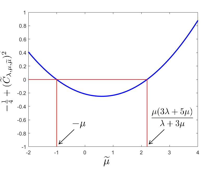
Figure 1: Blue lines: values of $\widetilde{C}_{\lambda,\mu,\widetilde{\mu}}$ and $-\frac{1}{4}+(\widetilde{C}_{\lambda,\mu,\widetilde{\mu}})^{2}$ with respect to $\widetilde{\mu}$. Here, $\mu=1$, $\lambda=2$.

Unfortunately, the generalized elastic Calderón relation for the closed-surface problem does not hold for the open-surface case any more, see Section 4.1. Before discussing the corresponding Calderón relation for the open-surface problem, we provide with some useful formulations in the closed-surface case which can be extended to the open-surface case for certain weighted integral operators introduced in Section 4.1. Let $N_{0}$ be the corresponding elastic hyper-singular operator in the zero-frequency case $\omega=0$ which is given by

$$N_{0}[\phi](x)=\widetilde{T}(\partial_{x},\nu_{x})\int_{\Gamma}(\widetilde{T}(\partial_{y},\nu_{y})\Pi_{0}(x,y))^{\top}\phi(y)ds_{y},\quad x\in\Gamma.$$ (3.7)

Lemma 3.5.

The hyper-singular operator $N_{0}$ can be reformulated as

$$N_{0}[\phi](x)=\partial_{\tau_{x}}V_{0}[\partial_{\tau}\phi](x),$$ (3.8)

where the integral operator $V_{0}:H^{-1/2}(\Gamma)^{2}\rightarrow H^{1/2}(\Gamma)^{2}$ is defined as

$$V_{0}[\chi](x)=\int_{\Gamma}\left[-C_{\lambda,\mu,\widetilde{\mu}}^{(1)}\ln|x-y|\mathbb{I}+C_{\lambda,\mu,\widetilde{\mu}}^{(2)}\frac{(x-y)(x-y)^{\top}}{|x-y|^{2}}\right]\chi(y)ds_{y},$$

where

$$C_{\lambda,\mu,\widetilde{\mu}}^{(1)} = -\frac{(\widetilde{\mu}+\mu)[(\lambda+\mu)(\widetilde{\mu}-3\mu)+2\mu(\widetilde{\mu}-\mu)]}{4\pi\mu(\lambda+2\mu)},$$

$$C_{\lambda,\mu,\widetilde{\mu}}^{(2)} = \frac{(\lambda+\mu)(\widetilde{\mu}+\mu)^{2}}{4\pi\mu(\lambda+2\mu)}.$$

Proof.

The proof of this lemma follows from the same steps as [25, Lemma 2.2.3] and is omitted here. ∎

Remark 3.6.

If $\widetilde{\mu}=\mu$, then $C_{\lambda,\mu,\widetilde{\mu}}^{(1)}=-C_{\lambda,\mu,\widetilde{\mu}}^{(2)}=\frac{\mu(\lambda+\mu)}{\pi(\lambda+2\mu)}$ and (3.8) is exactly the regularized formulation [25, (2.2.32)]. If $\widetilde{\mu}=-\mu$, then $N_{0}=0$. If $\widetilde{\mu}=\frac{\mu(3\lambda+5\mu)}{\lambda+3\mu}$ which means that $C_{\lambda,\mu,\widetilde{\mu}}^{(1)}=0$, it follows that the kernel of $V_{0}$ is bounded!

Lemma 3.7.

The hyper-singular boundary integral operator $N_{\omega}$ can be expressed alternatively as

$$N_{\omega}[\psi](x)$$ (3.9)

$$= -\int_{\Gamma}\left[\rho\omega^{2}(\nu_{x}\nu_{y}^{\top}-\nu_{x}^{\top}\nu_{y}I)G_{k_{s}}(x,y)-\widetilde{\mu}k_{s}^{2}G_{k_{s}}(x,y)J_{\nu_{x},\nu_{y}}-\rho\omega^{2}G_{k_{p}}(x,y)\nu_{x}\nu_{y}^{\top}\right]\psi(y)ds_{y}$$

$$+(\mu+\widetilde{\mu})^{2}\partial_{\tau_{x}}\int_{\Gamma}A\Pi_{\omega}(x,y)A\partial_{\tau_{y}}\psi(y)ds_{y}$$

$$+2(\mu+\widetilde{\mu})\partial_{\tau_{x}}\int_{\Gamma}G_{k_{s}}(x,y)\partial_{\tau_{y}}\psi(y)ds_{y}$$

$$-(\mu+\widetilde{\mu})\int_{\Gamma}\nu_{x}\nabla_{x}^{\top}[G_{k_{s}}(x,y)-G_{k_{p}}(x,y)]A\partial_{\tau_{y}}\psi(y)ds_{y}$$

$$-(\mu+\widetilde{\mu})\partial_{\tau_{x}}\int_{\Gamma}A\nabla_{y}[G_{k_{s}}(x,y)-G_{k_{p}}(x,y)]\nu_{y}^{\top}\psi(y)ds_{y}.$$

Proof.

This result is a generalized form of [37, Theorem 6.2] and the proof is also omitted. ∎

4 Calderón relation: open-surface

In this section, we study the elastic Calderón relation in the open-surface case. However, unlike the closed-surface case, an appropriate functional setting for the investigation of the composite operator $N_{\omega}S_{\omega}$ defined on an open-arc $\Gamma$ seems to be non-existing. As demonstrated in [27, Appendix B], even for the simplest open-surface–straight arc $\{x_{1}\in[-1,1],x_{2}=0\}$, the acoustic composite operator $N_{\omega}S_{\omega}$ maps the constant function with value $1$ into a function possessing $d^{-1}$ edge singularity which does not belong to $H^{-1/2}(\Gamma)$, where $d=d(x)$ denotes the distance between $x$ and the corresponding end point for any $x$ in a neighbourhood of each end point. This difficulty also appears in the elastic open-surface case since both the acoustic and elastic integral operators $N_{\omega},S_{\omega}$ defined on the straight arc contain similar singular kernels.

4.1 Weighted integral operators

Instead of studying the operators $N_{\omega},S_{\omega}$, we discuss the weighted forms $N_{\omega}^{\rm w},S_{\omega}^{\rm w}$ resulting from certain regularity of potentials. Let $\Gamma$ be a smooth open arc in ${\mathbb{R}}^{2}$ and the unbounded domain ${\mathbb{R}}^{2}\backslash\Gamma$ is fulfilled with a linear isotropic and homogeneous elastic medium. Then the time-harmonic problem of elastic scattering by an open-surface can be modeled by the Navier equation

$$\Delta^{*}u+\rho\omega^{2}u=0\quad\mbox{in}\quad{\mathbb{R}}^{2}\backslash\Gamma,$$ (4.1)

together with the boundary conditions

$$\begin{cases}\mbox{Dirichlet}:&u=F\cr\mbox{Neumann}:&\widetilde{T}(\partial,\nu)u=G\end{cases}\quad\mbox{on}\quad\Gamma,$$ (4.2)

and the Kupradze radiation condition at infinity [26]. Here, $u=(u_{1},u_{2})^{\top}$ denotes the displacement field.

Lemma 4.1.

The open-arc elastic scattering problem (4.1)-(4.2) has at most one solution.

Proof.

The proof of this result can be completed following the variational approach [35] together the generalized Rellich’s lemma in elasticity (see [3, Lemma 2.14]). ∎

It is known that [33, 35] the solutions of the Dirichlet and Neumann elastic problems of scattering by an open-arc admit the representations in forms of single- and double-layer potentials, respectively, i.e.,

$$u(x)=(\mathcal{S}_{\omega}\phi)(x):=\int_{\Gamma}\Pi_{\omega}(x,y))\phi(y)\,ds_{y},\quad\forall\,x\in{\mathbb{R}}^{2}\backslash\Gamma,$$ (4.3)

and

$$u(x)=(\mathcal{D}_{\omega}\psi)(x):=\int_{\Gamma}(\widetilde{T}(\partial_{y},\nu_{y})\Pi_{\omega}(x,y))^{\top}\psi(y)\,ds_{y},\quad\forall\,x\in{\mathbb{R}}^{2}\backslash\Gamma,$$ (4.4)

respectively. Then the Dirichlet and Neumann problems reduce to the boundary integral equations

$$S_{\omega}[\phi]=F,\quad N_{\omega}[\psi]=G\quad\mbox{on}\quad\Gamma.$$ (4.5)

Definition 4.2.

An operator $L$ between two Sobolev spaces is called bicontinuous if it is continuous and invertible. As a corollary, the inverse $L^{-1}$ is also continuous. Assume that $\Gamma\subset\partial\Omega$ where $\partial\Omega$ is a smooth boundary of a bounded domain $\Omega$ in ${\mathbb{R}}^{2}$. We denote by $\widetilde{H}^{s}(\Gamma)$ the space of all $f\in H^{s}(\Gamma)$ satisfying ${\rm supp}(f)\subseteq\overline{\Gamma}$.

Lemma 4.3.

The operators $S_{\omega}:\widetilde{H}^{-1/2}(\Gamma)^{2}\rightarrow H^{1/2}(\Gamma)$ and $N_{\omega}:\widetilde{H}^{1/2}(\Gamma)^{2}\rightarrow H^{-1/2}(\Gamma)$ are bicontinuous under the assumption that

$$\widetilde{\mu}\neq-\mu\quad\mbox{and}\quad\widetilde{\mu}\neq\frac{\mu(3\lambda+5\mu)}{\lambda+3\mu}.$$ (4.6)

Proof.

The bicontinuity of the operator $S_{\omega}$ holds analogously to [33]. The assumption (4.6) of $\widetilde{\mu}$ gives $C_{\lambda,\mu,\widetilde{\mu}}^{(1)}\neq 0$. By the integration kernel of $N_{\omega}$ together with the singularity decomposition (A.2), it can be deduced that the coefficient of the weakly-singular part in the term

$$(\mu+\widetilde{\mu})^{2}A\Pi_{\omega}(x,y)A+2(\mu+\widetilde{\mu})G_{k_{s}}(x,y)\mathbb{I}$$

is non-zero. Following the proof of the solvability of the hyper-singular operator [35, (3.6)] results into the bicontinuity of the operator $N_{\omega}$. ∎

Assumption 4.1.

In the rest of this work, we always assume the value of $\widetilde{\mu}$ to be such that (4.6) and additionally, $C_{\lambda,\mu,\widetilde{\mu}}^{(1)}\ln 2+C_{\lambda,\mu,\widetilde{\mu}}^{(2)}\neq 0$ hold.

Denote by $d=d(x)$ a non-negative smooth function for $x\in\Gamma$ to represent the distance between $x$ and the corresponding end point for any $x$ in a neighbourhood of each end point. Assuming that the right-hand sides $F,G$ in (4.5) are both infinitely differentiable, it is known [18] that the density functions $\phi,\psi$ in (4.5) can be expressed in the forms

$$\phi=\frac{\phi^{\rm{w}}}{w},\quad\psi=w\;\psi^{\rm{w}},$$ (4.7)

where $w=w(x)$ denotes a smooth function that reproduces the asymptotic $w\sim\sqrt{d}$ as $d\rightarrow 0$. It implies that $w/\sqrt{d}$ is infinitely differentiable up to the endpoints, and the new solutions $\phi^{\mbox{w}},\psi^{\mbox{w}}$ are smooth up to the end points of $\Gamma$. Taking into account the solution singularities (4.7), we obtain the new boundary integral equations

$$S_{\omega}^{\rm{w}}[\phi^{\rm{w}}]=F,\quad N_{\omega}^{\rm{w}}[\psi^{\rm{w}}]=G\quad\mbox{on}\quad\Gamma,$$ (4.8)

where the weighted integral operators $S_{\omega}^{\rm{w}},N_{\omega}^{\rm{w}}$ are defined as

$$S_{\omega}^{\rm{w}}[\phi^{\rm{w}}]=S_{\omega}\left[\frac{\phi^{\rm{w}}}{w}\right],\quad N_{\omega}^{\rm{w}}[\psi^{\rm{w}}]=N_{\omega}\left[w\;\psi^{\rm{w}}\right].$$

A similar regularized formulation of $N_{\omega}^{\rm{w}}$ can be obtained from (3.9) since the weight function $w$ in $N_{\omega}^{\mbox{w}}$ is smooth boundary-vanishing, see (4.19).

Without loss of generality, suppose that the boundary $\Gamma$ can be parameterized by means of a smooth vector function $x=x(t)=(x_{1}(t),x_{2}(t)),t\in[-1,1]$ satisfying $\mathcal{J}(t)=|x^{\prime}(t)|\neq 0$. Here the prime ^′ denotes the derivative with respect to $t$. Choosing the smooth weighting function $w$ as $w(t)=\sqrt{1-t^{2}}$ yields

$$S_{\omega}^{\rm{w}}[\phi^{\rm{w}}](x(t))=\int_{-1}^{1}\Pi_{\omega}(x(t),x(\iota))\frac{\phi^{\rm{w}}(x(\iota))}{\sqrt{1-\iota^{2}}}\mathcal{J}(\iota)d\iota.$$

Then utilizing the changes of variables $t=\cos\theta,\iota=\cos\vartheta$ leads us to

$$\widetilde{S}_{\omega}^{\rm{w}}[\widetilde{\phi}^{\mbox{w}}](\theta)=F(x(\cos\theta)),\quad\widetilde{\phi}^{\rm{w}}(\theta)=\phi^{\mbox{w}}(x(\cos\theta)),$$

where the operator $\widetilde{S}_{\omega}^{\rm{w}}$ is given by

$$\widetilde{S}_{\omega}^{\rm{w}}[\widetilde{\phi}^{\rm{w}}](\theta)=\int_{0}^{\pi}\Pi_{\omega}(x(\cos\theta),x(\cos\vartheta))\widetilde{\phi}^{\rm{w}}(\vartheta)\mathcal{J}(\cos\vartheta)d\vartheta.$$

The parameterized form $\widetilde{N}_{\omega}^{\rm{w}}$ corresponding to the integral operator $N_{\omega}^{\rm{w}}$ can be deduced in a similar manner.

Note that each smooth $\cos\theta$ dependence function can be extended to be a $2\pi$-periodic and even function. To study the properties of the parameterized operators $\widetilde{S}_{\omega}^{\rm{w}},\widetilde{N}_{\omega}^{\rm{w}}$, we define the following Sobolev spaces:

Definition 4.4.

For $s\in{\mathbb{R}}$, the Sobolev space $H^{s}_{e}(2\pi)$ is defined as the completion of space of infinitely differentiable $2\pi$-periodic and even functions defined in the real line with respect to the norm

$$\|v\|_{H^{s}_{e}(2\pi)}^{2}=|a_{0}|^{2}+2\sum_{m\in{\mathbb{Z}}^{+}}m^{2s}|a_{m}|^{2},$$

where $a_{m},m\in{\mathbb{Z}}^{+}$ denotes the coefficients in the cosine expansion of $v$:

$$v(\theta)=\frac{1}{2}a_{0}+\sum_{m\in{\mathbb{Z}}^{+}}a_{m}\cos(m\theta).$$

4.2 Calderón relation: straight arc

Let $\Gamma$ be, specially, the straight arc $\{x_{1}\in[-1,1],x_{2}=0\}$ which means that $x_{1}(t)=t,x_{2}(t)=0,t\in[-1,1]$ for $x\in\Gamma$ and $|x^{\prime}(t)|=1$. In this subsection, we consider the operators $\widetilde{S}_{\omega}^{\rm{w}},\widetilde{N}_{\omega}^{\rm{w}}$ on the straight arc at zero frequency that are denoted by $\widetilde{S}_{0},\widetilde{N}_{0}$, i.e.,

$$\widetilde{S}_{0}[\gamma](\theta)=\int_{0}^{\pi}\left[-C_{\lambda,\mu}^{(1)}\ln|\cos\theta-\cos\vartheta|\mathbb{I}+C_{\lambda,\mu}^{(2)}\begin{pmatrix}1&0\\ 0&0\end{pmatrix}\right]\gamma(\vartheta)d\vartheta,$$ (4.9)

and

$$\widetilde{N}_{0}=\widetilde{D}_{0}\widetilde{V}_{0}\widetilde{T}_{0},$$ (4.10)

where

$$\widetilde{D}_{0}[\gamma](\theta)=\frac{1}{\sin\theta}\frac{d\gamma(\theta)}{d\theta},\quad\widetilde{T}_{0}[\gamma](\theta)=\frac{d}{d\theta}(\gamma(\theta)\sin\theta),$$

$$\widetilde{V}_{0}[\gamma](\theta)=\int_{0}^{\pi}\left[-C_{\lambda,\mu,\widetilde{\mu}}^{(1)}\ln|\cos\theta-\cos\vartheta|\mathbb{I}+C_{\lambda,\mu,\widetilde{\mu}}^{(2)}\begin{pmatrix}1&0\\ 0&0\end{pmatrix}\right]\gamma(\vartheta)d\vartheta.$$

The expression of $\widetilde{N}_{0}$ follows immediately from Lemma 3.5 thanks to the smooth boundary-vanishing weight $w$.

For the basis $\{e_{n}=\cos n\theta:n\in{\mathbb{N}}\}$ of $H^{s}_{e}(2\pi),s\geq 0$, it can be derived from the diagonal property of Symm’s operator [29] that

$$\widetilde{S}_{0}[e_{n}]=\begin{pmatrix}\lambda_{1,n}^{S}&\\ &\lambda_{2,n}^{S}\end{pmatrix}e_{n},$$ (4.11)

$$\lambda_{1,n}^{S}=\begin{cases}\pi(C_{\lambda,\mu}^{(1)}\ln 2+C_{\lambda,\mu}^{(2)}),&n=0,\cr\frac{\pi C_{\lambda,\mu}^{(1)}}{n},&n\geq 1,\end{cases}\quad\lambda_{2,n}^{S}=\begin{cases}\pi C_{\lambda,\mu}^{(1)}\ln 2,&n=0,\cr\lambda_{1,n}^{S},&n\geq 1,\end{cases}$$

and

$$\widetilde{V}_{0}[e_{n}]=\begin{pmatrix}\lambda_{1,n}^{V}&\\ &\lambda_{2,n}^{V}\end{pmatrix}e_{n},$$ (4.12)

$$\lambda_{1,n}^{V}=\begin{cases}\pi(C_{\lambda,\mu,\widetilde{\mu}}^{(1)}\ln 2+C_{\lambda,\mu,\widetilde{\mu}}^{(2)}),&n=0,\cr\frac{\pi C_{\lambda,\mu,\widetilde{\mu}}^{(1)}}{n},&n\geq 1,\end{cases}\quad\lambda_{2,n}^{V}=\begin{cases}\pi C_{\lambda,\mu,\widetilde{\mu}}^{(1)}\ln 2,&n=0,\cr\lambda_{1,n}^{V},&n\geq 1.\end{cases}$$

For $n=0$, we can obtain from (4.12) that

$$\widetilde{N}_{0}[e_{0}]=\widetilde{D}_{0}\widetilde{V}_{0}\widetilde{T}_{0}[e_{0}]=\widetilde{D}_{0}\widetilde{V}_{0}[e_{1}]=\widetilde{D}_{0}[\lambda_{1,1}^{V}\mathbb{I}e_{1}]=-\pi C_{\lambda,\mu,\widetilde{\mu}}^{(1)}\mathbb{I}.$$

For $n=1$, it follows that

$$\widetilde{N}_{0}[e_{1}](\theta)=\widetilde{D}_{0}\widetilde{V}_{0}[e_{2}](\theta)=\widetilde{D}_{0}[\lambda_{1,2}^{V}\mathbb{I}e_{2}](\theta)=-2\pi C_{\lambda,\mu,\widetilde{\mu}}^{(1)}\mathbb{I}\cos\theta.$$

For $n\geq 2$, note that

$$\widetilde{T}_{0}[e_{n}](\theta) = \cos\theta\cos n\theta-n\sin n\theta\sin\theta$$

$$= \frac{e_{n+1}+e_{n-1}}{2}+n\frac{e_{n+1}-e_{n-1}}{2}.$$

A direct application of (4.12) implies

$$\widetilde{V}_{0}\widetilde{T}_{0}[e_{n}] = \pi C_{\lambda,\mu,\widetilde{\mu}}^{(1)}\left(\frac{\frac{1}{n+1}e_{n+1}+\frac{1}{n-1}e_{n-1}}{2}+n\frac{\frac{1}{n+1}e_{n+1}-\frac{1}{n-1}e_{n-1}}{2}\right)\mathbb{I}$$

$$= \frac{\pi C_{\lambda,\mu,\widetilde{\mu}}^{(1)}}{2}(e_{n+1}-e_{n-1})$$

and then further for $n\geq 2$ we have

$$\widetilde{N}_{0}[e_{n}](\theta)=-\pi C_{\lambda,\mu,\widetilde{\mu}}^{(1)}\left(\frac{\cos\theta\sin n\theta}{\sin\theta}+n\cos n\theta\right)\mathbb{I},$$ (4.13)

which also holds for $n=1$.

For the operators $\widetilde{D}_{0},\widetilde{T}_{0}$, we have the following basic result, see [27].

Lemma 4.5.

The operators $\widetilde{D}_{0}:H^{2}_{e}(2\pi)\rightarrow H^{0}_{e}(2\pi)$ and $\widetilde{T}_{0}:H^{2}_{e}(2\pi)\rightarrow H^{1}_{e}(2\pi)$ are bounded.

The properties of the operators $\widetilde{S}_{0},\widetilde{N}_{0},\widetilde{J}_{0}$ are presented in the following theorem.

Theorem 4.6.

For all $s\geq 0$, the operators $\widetilde{S}_{0},\widetilde{V}_{0}:H^{s}_{e}(2\pi)^{2}\rightarrow H^{s+1}_{e}(2\pi)^{2}$, $\widetilde{N}_{0}:H^{s+1}_{e}(2\pi)^{2}\rightarrow H^{s}_{e}(2\pi)^{2}$ and $\widetilde{J}_{0}=\widetilde{N}_{0}\widetilde{S}_{0}:H^{s}_{e}(2\pi)^{2}\rightarrow H^{s}_{e}(2\pi)^{2}$ are all bicontinuous.

Proof.

• Bicontinuity of $\widetilde{S}_{0},\widetilde{V}_{0}$:

For $f=\sum_{n\in{\mathbb{N}}}f_{n}e_{n}\in H^{s}_{e}(2\pi)^{2}$, let the operators $W_{S},W_{V}$ be defined as

$$W_{S}[f]=\sum_{n\in{\mathbb{N}}}\begin{pmatrix}\lambda_{1,n}^{S}&\\ &\lambda_{2,n}^{S}\end{pmatrix}f_{n}e_{n},\quad W_{V}[f]=\sum_{n\in{\mathbb{N}}}\begin{pmatrix}\lambda_{1,n}^{V}&\\ &\lambda_{2,n}^{V}\end{pmatrix}f_{n}e_{n}.$$

Under the assumption (4.1), it follows that $W_{S},W_{V}:H^{s}_{e}(2\pi)^{2}\rightarrow H^{s+1}_{e}(2\pi)^{2}$ are bicontinuous for all $s\geq 0$. In particular, $W_{S},W_{V}$ are continuous from $H^{0}_{e}(2\pi)^{2}$ into $H^{0}_{e}(2\pi)^{2}$. For every basis element $e_{n},n\in{\mathbb{N}}$, the operators $\widetilde{S}_{0},\widetilde{V}_{0}$ coincide with $W_{S},W_{V}$, respectively. Then $\widetilde{S}_{0}$ (resp. $\widetilde{V}_{0}$) and $W_{S}$ (resp. $W_{V}$) coincide on the dense set $\{e_{n}\}$ of $H^{0}_{e}(2\pi)^{2}$ and thus, coincide throughout $H^{0}_{e}(2\pi)^{2}$. Then the bicontinuity of $\widetilde{S}_{0},\widetilde{V}_{0}:H^{s}_{e}(2\pi)^{2}\rightarrow H^{s+1}_{e}(2\pi)^{2}$ follows immediately.

• Bicontinuity of $\widetilde{J}_{0}$:

We first show that $\widetilde{J}_{0}:H^{s}_{e}(2\pi)^{2}\rightarrow H^{s}_{e}(2\pi)^{2}$ is continuous. Obviously, $\widetilde{J}_{0}:H^{1}_{e}(2\pi)^{2}\rightarrow H^{0}_{e}(2\pi)^{2}$ is continuous since $\widetilde{D}_{0}:H^{2}_{e}(2\pi)\rightarrow H^{0}_{e}(2\pi)$ [27, Lemma 3.2] and $\widetilde{T}_{0}:H^{2}_{e}(2\pi)\rightarrow H^{1}_{e}(2\pi)$ are continuous. Combining the relations (4.11) and (4.13) gives

$$\widetilde{J}_{0}[e_{n}](\theta)=\begin{cases}\begin{pmatrix}\lambda_{1}^{J}&\\ &\lambda_{2}^{J}\end{pmatrix},&n=0,\cr\lambda_{3}^{J}\left(\frac{\cos\theta\sin n\theta}{n\sin\theta}+\cos n\theta\right)\mathbb{I},&n\geq 1,\end{cases}$$ (4.14)

where $\lambda_{1}^{J}=-\pi^{2}C_{\lambda,\mu,\widetilde{\mu}}^{(1)}(C_{\lambda,\mu}^{(1)}\ln 2+C_{\lambda,\mu}^{(2)})$, $\lambda_{2}^{J}=-\pi^{2}C_{\lambda,\mu,\widetilde{\mu}}^{(1)}C_{\lambda,\mu}^{(1)}\ln 2$ and $\lambda_{3}^{J}=-\pi^{2}C_{\lambda,\mu,\widetilde{\mu}}^{(1)}C_{\lambda,\mu}^{(1)}$ for $n\geq 1$. Let the operator $\widetilde{C}$ be given by

$$\widetilde{C}[\gamma](\theta)=\frac{\theta(\pi-\theta)}{\pi\sin\theta}\left[\frac{1}{\theta}\int_{0}^{\theta}\gamma(s)ds-\frac{1}{\pi-\theta}\int_{\theta}^{\pi}\gamma(s)ds\right].$$ (4.15)

It has been proved in  [27, Lemma 3.5] that the operator $\widetilde{C}:H^{s}_{e}(2\pi)\rightarrow H^{s}_{e}(2\pi)$ is continuous and

$$\widetilde{C}[e_{n}](\theta)=\begin{cases}0,&n=0,\cr\frac{\sin n\theta}{n\sin\theta},&n\geq 1.\end{cases}$$ (4.16)

Then we can rewrite $\widetilde{J}_{0}[e_{n}]$ as

$$\widetilde{J}_{0}[e_{n}]=\widetilde{W}_{0}[e_{n}],$$

where the integral operator $\widetilde{W}_{0}$ is defined as

$$\widetilde{W}_{0}[\gamma](\theta)=\lambda_{3}^{J}\mathbb{I}\gamma(\theta)+\lambda_{3}^{J}\cos\theta\mathbb{I}\widetilde{C}[\gamma](\theta)+\frac{1}{\pi}\begin{pmatrix}\lambda_{1}^{J}-\lambda_{3}^{J}&\\ &\lambda_{2}^{J}-\lambda_{3}^{J}\end{pmatrix}\int_{0}^{\pi}\gamma(s)ds.$$

The continuity of $\widetilde{W}_{0}:H^{s}_{e}(2\pi)\rightarrow H^{s}_{e}(2\pi)$ deduces from the continuity of $\widetilde{C}:H^{s}_{e}(2\pi)\rightarrow H^{s}_{e}(2\pi)$ for all $s\geq 0$ and therefore the continuity of $\widetilde{J}_{0}:H^{s}_{e}(2\pi)\rightarrow H^{s}_{e}(2\pi)$ results.

Next we prove the invertibility of $\widetilde{J}_{0}$ and its inverse $\widetilde{J}_{0}^{-1}:H^{s}_{e}(2\pi)^{2}\rightarrow H^{s}_{e}(2\pi)^{2}$ is given by

$$\widetilde{J}_{0}^{-1}=-\left(\pi^{2}(C_{\lambda,\mu,\widetilde{\mu}}^{(1)})^{2}\right)^{-1}\widetilde{S}_{0}^{-1}\widetilde{C}\widetilde{V}_{0}\widetilde{T}_{0},$$ (4.17)

for $s\geq 2$ and given by the unique continuous extension of the right-hand side of (4.17) for $0\leq s<2$. On one hand, it easily follows from [27, Corollary 3.13] that $\widetilde{C}\widetilde{V}_{0}\widetilde{T}_{0}:H^{s}_{e}(2\pi)^{2}\rightarrow H^{s}_{e}(2\pi)^{2},s\geq 1$ is continuous and it can be extended in a unique style to an operator which is continuous from $H^{s}_{e}(2\pi)^{2}$ to $H^{s+1}_{e}(2\pi)^{2}$ for all $s\geq 0$. For $n=0$, $\widetilde{D}_{0}[e_{0}]=0$. For $n\geq 1$,

$$\widetilde{D}_{0}[e_{n}]=-n\frac{\sin n\theta}{\sin\theta}.$$

Note that for $n\geq 1$,

$$\widetilde{V}_{0}[e_{n}]=\lambda_{1,n}^{V}\mathbb{I}[e_{n}],\quad\widetilde{C}[e_{n}]=\frac{\sin n\theta}{n\sin\theta}.$$

We conclude from the density of the basis $\{e_{n}\}$ in $H^{s}_{e}(2\pi)$ that

$$\widetilde{D}_{0}\mathbb{I}=-\pi^{2}(C_{\lambda,\mu,\widetilde{\mu}}^{(1)})^{2}\widetilde{C}(\widetilde{V}_{0}^{-1})^{2}.$$

This means that $\widetilde{D}_{0}:H^{s+2}_{e}(2\pi)\rightarrow H^{s}_{e}(2\pi),s\geq 0$ is continuous. Denote

$$\widetilde{I}_{0}=-\left(\pi^{2}(C_{\lambda,\mu,\widetilde{\mu}}^{(1)})^{2}\right)^{-1}\widetilde{S}_{0}^{-1}\widetilde{C}\widetilde{V}_{0}\widetilde{T}_{0}.$$

Then

$$\widetilde{J}_{0}\widetilde{I}_{0}=\widetilde{C}\widetilde{V}_{0}^{-1}\widetilde{V}_{0}^{-1}\widetilde{V}_{0}\widetilde{T}_{0}\widetilde{S}_{0}\widetilde{S}_{0}^{-1}\widetilde{C}\widetilde{V}_{0}\widetilde{T}_{0}=\widetilde{C}\widetilde{V}_{0}^{-1}\widetilde{T}_{0}\widetilde{C}\widetilde{V}_{0}\widetilde{T}_{0}$$

with regularity

$$H^{s}_{e}(2\pi)^{2}\xrightarrow{\widetilde{C}\widetilde{V}_{0}\widetilde{T}_{0}}H^{s+1}_{e}(2\pi)^{2}\xrightarrow{\widetilde{T}_{0}}H^{s}_{e}(2\pi)^{2}\xrightarrow{\widetilde{V}_{0}^{-1}}H^{s-1}_{e}(2\pi)^{2}\xrightarrow{\widetilde{C}}H^{s-1}_{e}(2\pi)^{2},\quad s\geq 1.$$

Noting that $\widetilde{T}_{0}[e_{0}]=e_{1}$, $\widetilde{C}[e_{1}]=e_{0}$ and $\widetilde{T}_{0}\widetilde{C}[e_{n}]=e_{n}$ for all $n\geq 1$, we obtain $\widetilde{J}_{0}\widetilde{I}_{0}=I$ which means that $\widetilde{I}_{0}$ is a right inverse of $\widetilde{J}_{0}$ for $s\geq 1$. On the other hand, for $s\geq 2$,

$$\widetilde{I}_{0}\widetilde{J}_{0}=\widetilde{S}_{0}^{-1}\widetilde{C}\widetilde{V}_{0}\widetilde{T}_{0}\widetilde{C}\widetilde{V}_{0}^{-1}\widetilde{V}_{0}^{-1}\widetilde{V}_{0}\widetilde{T}_{0}\widetilde{S}_{0}=\widetilde{S}_{0}^{-1}\widetilde{C}\widetilde{V}_{0}\widetilde{T}_{0}\widetilde{C}\widetilde{V}_{0}^{-1}\widetilde{T}_{0}\widetilde{S}_{0},$$

Using the same argument for right inverse demonstration, it can be obtained that

$$\widetilde{I}_{0}\widetilde{J}_{0}=\widetilde{S}_{0}^{-1}\widetilde{C}\widetilde{T}_{0}\widetilde{S}_{0}.$$

Definition of the operators $\widetilde{C},\widetilde{T}_{0}$ yields $\widetilde{C}\widetilde{T}_{0}[f]=f$ for all $f\in H^{s}_{e}(2\pi)$. Thus, $\widetilde{I}_{0}\widetilde{J}_{0}=I$ which means that $\widetilde{I}_{0}$ is a left inverse of $\widetilde{J}_{0}$ for $s\geq 2$. The continuity of $\widetilde{I}_{0}:H^{s}_{e}(2\pi)^{2}\rightarrow H^{s}_{e}(2\pi)^{2}$ for $s\geq 2$, which can be extended in a unique style as a continuous operator for $s\geq 0$, follows immediately from the continuity of $\widetilde{S}_{0}$ and $\widetilde{C}\widetilde{V}_{0}\widetilde{T}_{0}$. Therefore, the relations $\widetilde{J}_{0}\widetilde{I}_{0}=I$ and $\widetilde{I}_{0}\widetilde{J}_{0}=I$ can be extended to the case of $s\geq 0$ due to the density of $H^{2}_{e}(2\pi)$ in $H^{s}_{e}(2\pi)$, $0\leq s<2$. This completes the proof of the bicontinuity of $\widetilde{J}_{0}$.

• Bicontinuity of $\widetilde{N}_{0}$:

The bicontinuity of $\widetilde{N}_{0}:H^{s+1}_{e}(2\pi)^{2}\rightarrow H^{s}_{e}(2\pi)^{2}$ results from the bicontinuity of $\widetilde{S}_{0},\widetilde{J}_{0}$ and $\widetilde{N}_{0}=\widetilde{J}_{0}\widetilde{S}_{0}^{-1}$. ∎

Theorem 4.7.

For all $s>0$, the point spectrum $\sigma_{s}$ of $\widetilde{J}_{0}$ can be expressed as the union

$$\sigma_{s}=\Lambda_{s}\cup\Lambda_{\infty},$$

where $\Lambda_{s}$ is the open bounded set

$$\Lambda_{s}=\left\{\leftthreetimes=-\lambda_{3}^{J}(\lambda_{x}+i\lambda_{y})\in{\mathbb{C}}:s+\frac{1}{2}<\frac{-(\lambda_{x}+1)}{(\lambda_{x}+1)^{2}+\lambda_{y}^{2}},\lambda_{x}+1<0\right\},$$

and $\Lambda_{\infty}$ is the discrete set

$$\Lambda_{\infty}=\left\{\lambda_{1}^{J},\lambda_{2}^{J},\lambda_{3}^{J}+\frac{\lambda_{3}^{J}}{n}:n\in{\mathbb{N}}\right\}.$$

Moreover, $\sigma_{s}$ is bounded away from zero and infinity.

Proof.

Rewriting (4.14) gives

$$\widetilde{J}_{0}[e_{n}]=\begin{cases}\begin{pmatrix}\lambda_{1}^{J}&\\ &\lambda_{2}^{J}\end{pmatrix},&n=0,\cr-4\lambda_{3}^{J}\widetilde{j}_{0}[e_{n}]\mathbb{I},&n\geq 1,\end{cases}$$ (4.18)

where

$$\widetilde{j}_{0}[e_{n}](\theta)=-\frac{\sin(n+1)\theta}{4n\sin\theta}+\frac{\cos n\theta}{4n}-\frac{\cos n\theta}{4},\quad n\geq 1.$$

Then the point spectrum of $\widetilde{J}_{0}$ results from [27, Lemma 3.16]. Utilizing the polar coordinates $(r,\theta)$ around $(-1,0)$ the set $\Lambda_{s}$ can be rewritten as

$$\Lambda_{s}=\left\{\leftthreetimes=-\lambda_{3}^{J}(\lambda_{x}+i\lambda_{y})\in{\mathbb{C}}:\lambda_{x}+1=r\cos\theta,\lambda_{y}=r\sin\theta,0<r<-\frac{\cos\theta}{s+\frac{1}{2}},\frac{\pi}{2}<\theta<\frac{3\pi}{2}\right\},$$

satisfying $\cap_{s>0}\lambda_{s}=\emptyset$ and $\cap_{s>0}\overline{\lambda_{s}}=\{\lambda_{3}^{J}\}$. Additionally, $\mbox{dist}(\sigma_{s},0)=|\lambda_{3}^{J}|$ and

$$\max_{\lambda\in\sigma_{s}}|\leftthreetimes|=\max\{|\lambda_{1}^{J}|,|\lambda_{2}^{J}|,3|\lambda_{3}^{J}|\}.$$

∎

Remark 4.8.

We point out in this remark that $\lambda_{3}^{J}=-\frac{1}{4}+(\widetilde{C}_{\lambda,\mu,\widetilde{\mu}})^{2}$ implying that the clustered point of the point spectrum of the Calderón formula $\widetilde{J}_{0}=\widetilde{N}_{0}\widetilde{S}_{0}$ (in the case of straight arc) is equivalent to the accumulation point of the eigenvalues of the Calderón formula in the closed-surface case (Theorem 3.4). In fact, on one hand,

$$\lambda_{3}^{J} = -\pi^{2}C_{\lambda,\mu,\widetilde{\mu}}^{(1)}C_{\lambda,\mu}^{(1)}$$

$$= \frac{(\widetilde{\mu}+\mu)[(\lambda+\mu)(\widetilde{\mu}-3\mu)+2\mu(\widetilde{\mu}-\mu)]}{4\mu(\lambda+2\mu)}\frac{\lambda+3\mu}{4\mu(\lambda+2\mu)}.$$

On the other hand,

$$-\frac{1}{4}+(\widetilde{C}_{\lambda,\mu,\widetilde{\mu}})^{2}=\left(\widetilde{C}_{\lambda,\mu,\widetilde{\mu}}-\frac{1}{2}\right)\left(\widetilde{C}_{\lambda,\mu,\widetilde{\mu}}+\frac{1}{2}\right).$$

Then the following direct evaluations

$$\widetilde{C}_{\lambda,\mu,\widetilde{\mu}}-\frac{1}{2}=\frac{2\mu\widetilde{\mu}+(\lambda+\mu)(\widetilde{\mu}-\mu)-2\mu(\lambda+2\mu)}{4\mu(\lambda+2\mu)}=\frac{(\lambda+\mu)(\widetilde{\mu}-3\mu)+2\mu(\widetilde{\mu}-\mu)}{4\mu(\lambda+2\mu)},$$

and

$$\widetilde{C}_{\lambda,\mu,\widetilde{\mu}}+\frac{1}{2}=\frac{2\mu\widetilde{\mu}+(\lambda+\mu)(\widetilde{\mu}-\mu)+2\mu(\lambda+2\mu)}{4\mu(\lambda+2\mu)}=\frac{(\widetilde{\mu}+\mu)(\lambda+3\mu)}{4\mu(\lambda+2\mu)},$$

indicate the argument.

4.3 Calderón relation: general open-surface

For a general smooth open-arc $\Gamma$, combining the Jacobian $\mathcal{J}(\theta)=|x^{\prime}(\cos\theta)|$ and the operators $\widetilde{S}_{0},\widetilde{N}_{0}$, we introduce the operators

$$\widetilde{S}_{0}^{\mathcal{J}}=\widetilde{S}_{0}\widetilde{Z}_{0},\quad\widetilde{N}_{0}^{\mathcal{J}}=\widetilde{Z}_{0}^{-1}\widetilde{N}_{0}$$

and $\widetilde{J}_{0}^{\mathcal{J}}=\widetilde{N}_{0}^{\mathcal{J}}\widetilde{S}_{0}^{\mathcal{J}}$, where the operator $\widetilde{Z}_{0}$ is given by $\widetilde{Z}_{0}[\gamma](\theta)=\gamma(\theta)\mathcal{J}(\theta)$. Note that $\widetilde{J}_{0}^{\mathcal{J}}=\widetilde{Z}_{0}^{-1}\widetilde{J}_{0}\widetilde{Z}_{0}$, the following results hold.

Corollary 4.9.

For all $s\geq 0$, the operators $\widetilde{S}_{0}^{\mathcal{J}}:H^{s}_{e}(2\pi)^{2}\rightarrow H^{s+1}_{e}(2\pi)^{2}$, $\widetilde{N}_{0}^{\mathcal{J}}:H^{s+1}_{e}(2\pi)^{2}\rightarrow H^{s}_{e}(2\pi)^{2}$ and $\widetilde{J}_{0}^{\mathcal{J}}:H^{s}_{e}(2\pi)^{2}\rightarrow H^{s}_{e}(2\pi)^{2}$ are all bicontinuous. Moreover, the point spectrum of $\widetilde{J}_{0}^{\mathcal{J}}$ is equivalent to the point spectrum of $\widetilde{J}_{0}$ for $s>0$.

The following lemma builds a relationship between the function spaces $H^{s}_{e}(2\pi),H^{s+1}_{e}(2\pi)$ and the original function spaces $\widetilde{H}^{-1/2}(\Gamma),\widetilde{H}^{1/2}(\Gamma)$, see [27, Corollary 4.3, Lemma 4.9].

Lemma 4.10.

For any $\widetilde{\phi}\in H^{s}_{e}(2\pi)$ and $\widetilde{\psi}\in H^{s+1}_{e}(2\pi)$ with $s>0$. Denote $\phi(t)=\widetilde{\phi}(\arccos(t)),\psi(t)=\widetilde{\psi}(\arccos(t)),t\in[-1,1]$. For all $x=x(t)\in\Gamma$, define $\alpha(x)=\phi(t)$, $\beta(x)=\psi(t)$ and $W(x)=w(t)$. Then we have $\alpha/W\in\widetilde{H}^{-1/2}(\Gamma)$ and $\beta W\in\widetilde{H}^{1/2}(\Gamma)$.

The generalized Calderón relations for elastic open-surface problem is summarized in the following theorem whose proof relies heavily on the singularity decompositions of the kernels of the integral operators as being stated in Appendix.

Theorem 4.11.

For all $s>0$, the operators $\widetilde{S}_{\omega}^{\rm{w}}:H^{s}_{e}(2\pi)^{2}\rightarrow H^{s+1}_{e}(2\pi)^{2}$, $\widetilde{N}_{\omega}^{\rm{w}}:H^{s+1}_{e}(2\pi)^{2}\rightarrow H^{s}_{e}(2\pi)^{2}$ and $\widetilde{J}_{\omega}^{\rm{w}}=\widetilde{N}_{0}\widetilde{S}_{0}:H^{s}_{e}(2\pi)^{2}\rightarrow H^{s}_{e}(2\pi)^{2}$ are all bicontinuous. Moreover, the following generalized Calderón relation

$$\widetilde{J}_{\omega}^{\rm{w}}=\widetilde{J}_{0}^{\mathcal{J}}+\widetilde{K}$$

holds, where $\widetilde{K}:H^{s}_{e}(2\pi)^{2}\rightarrow H^{s}_{e}(2\pi)^{2}$ is compact and $\widetilde{J}_{0}^{\mathcal{J}}:H^{s}_{e}(2\pi)^{2}\rightarrow H^{s}_{e}(2\pi)^{2}$ is bicontinuous and its point spectrum is given by $\sigma_{s}$, see Theorem 4.7.

Proof.

• Bicontinuity of $\widetilde{S}_{\omega}^{\rm{w}}$ and $\widetilde{V}_{\omega}^{\rm{w}}$:

For integer $s\geq 0$, in view of the singularity decomposition (A.1) of the fundamental solution $\Pi_{\omega}$ we know that

$$\widetilde{S}_{\omega}^{\rm{w}}[\gamma](\theta) = \widetilde{S}_{0}^{\mathcal{J}}[\gamma](\theta)+\sum_{n=2}^{s+3}A_{n}(\cos\theta)\int_{0}^{\pi}(\cos\theta-\cos\vartheta)^{n}\ln|\cos\theta-\cos\vartheta|\gamma(\vartheta)\mathcal{J}(\vartheta)d\vartheta$$

$$+\int_{0}^{\pi}\hat{A}_{s+3}(\cos\theta,\cos\vartheta)\gamma(\vartheta)\mathcal{J}(\vartheta)d\vartheta.$$

It follows from [27, Lemma 4.1] that $\widetilde{S}_{\omega}^{\rm{w}}-\widetilde{S}_{0}^{\mathcal{J}}$ maps continuously from $H^{s}_{e}(2\pi)^{2}$ into $H^{s+3}_{e}(2\pi)^{2}$ and this result can be extended to the case of all $s\geq 0$ by interpolation. Therefore, $\widetilde{S}_{\omega}^{\rm{w}}:H^{s}_{e}(2\pi)^{2}\rightarrow H^{s+1}_{e}(2\pi)^{2}$ is continuous. In view of the invertibility of $\widetilde{S}_{0}^{\mathcal{J}}$, the operator $\widetilde{S}_{\omega}^{\rm{w}}$ can be expressed as

$$\widetilde{S}_{\omega}^{\rm{w}}=\widetilde{S}_{0}^{\mathcal{J}}\left(I+(\widetilde{S}_{0}^{\mathcal{J}})^{-1}(\widetilde{S}_{\omega}^{\rm{w}}-\widetilde{S}_{0}^{\mathcal{J}})\right),$$

in which $(\widetilde{S}_{0}^{\mathcal{J}})^{-1}(\widetilde{S}_{\omega}^{\rm{w}}-\widetilde{S}_{0}^{\mathcal{J}}):H^{s}_{e}(2\pi)^{2}\rightarrow H^{s}_{e}(2\pi)^{2}$ is compact, i.e., the operator $(\widetilde{S}_{0}^{\mathcal{J}})^{-1}\widetilde{S}_{\omega}^{\rm{w}}$ is a compact perturbation of the identity operator. Then we conclude from the injectivity of $S_{\omega}$ together with Lemma 4.10 that the operator $(\widetilde{S}_{0}^{\mathcal{J}})^{-1}\widetilde{S}_{\omega}^{\rm{w}}$ is injective for $s>0$. Therefore, the bicontinuity of the operator $\widetilde{S}_{\omega}^{\rm{w}}:H^{s}_{e}(2\pi)^{2}\rightarrow H^{s+1}_{e}(2\pi)^{2},s>0$ follows immediately from the Fredholm alternative. Let the operator $\widetilde{V}_{\omega}^{\rm{w}}$ be defined as

$$\widetilde{V}_{\omega}^{\rm{w}}[\gamma](\theta)=\int_{0}^{\pi}\left[(\mu+\widetilde{\mu})^{2}A\Pi_{\omega}(x(\cos\theta),x(\cos\vartheta))A+2(\mu+\widetilde{\mu})G_{k_{s}}(x(\cos\theta),x(\cos\vartheta))\mathbb{I}\right]\gamma(\vartheta)d\vartheta.$$

In view of (A.2), it can be proved that $\widetilde{V}_{\omega}^{\rm{w}}-\widetilde{V}_{0}:H^{s}_{e}(2\pi)^{2}\rightarrow H^{s+3}_{e}(2\pi)^{2}$ and $\widetilde{V}_{\omega}^{\rm{w}}:H^{s}_{e}(2\pi)^{2}\rightarrow H^{s+1}_{e}(2\pi)^{2}$ are continuous for all $s\geq 0$. Analogous to $\widetilde{S}_{\omega}^{\rm{w}}$, it can be proved that $\widetilde{V}_{\omega}^{\rm{w}}:H^{s}_{e}(2\pi)^{2}\rightarrow H^{s+1}_{e}(2\pi)^{2},s>0$ is bicontinuous.

• Bicontinuity of $\widetilde{N}_{\omega}^{\rm{w}}$:

Extension of the regularized formula (3.9) to the open-surface case gives

$$\widetilde{N}_{\omega}^{\rm{w}}=\widetilde{N}_{\omega}^{\rm{g_{1}}}+\widetilde{N}_{\omega}^{\rm{g_{2}}}+\widetilde{N}_{\omega}^{\rm{pv}}$$ (4.19)

where

$$\widetilde{N}_{\omega}^{\rm{g_{1}}}[\gamma](\theta)=\int_{0}^{\pi}\Pi_{\omega}^{N}(x(\cos\theta),x(\cos\vartheta))\sin^{2}\vartheta\gamma(\vartheta)\mathcal{J}(\cos\vartheta)d\vartheta,$$

$$\widetilde{N}_{\omega}^{\rm{g_{2}}}[\gamma](\theta)=R_{1}\widetilde{T}_{0}[\gamma](\theta)+\widetilde{Z}_{0}^{-1}\widetilde{D}_{0}R_{2}[\gamma](\theta),$$

and

$$\widetilde{N}_{\omega}^{\rm{pv}}[\gamma](\theta)=\widetilde{Z}_{0}^{-1}\widetilde{D}_{0}\widetilde{V}_{\omega}^{\rm{w}}\widetilde{T}_{0}[\gamma](\theta).$$

Here,

$$\Pi_{\omega}^{N}(x,y)=-\rho\omega^{2}(\nu_{x}\nu_{y}^{\top}-\nu_{x}^{\top}\nu_{y}I)G_{k_{s}}(x,y)+\widetilde{\mu}k_{s}^{2}G_{k_{s}}(x,y)J_{\nu_{x},\nu_{y}}+\rho\omega^{2}G_{k_{p}}(x,y)\nu_{x}\nu_{y}^{\top},$$

and the operators $R_{1},R_{2}$ are given by

$$R_{1}[\gamma](\theta)=-(\mu+\widetilde{\mu})\int_{0}^{\pi}\nu_{x(\cos\theta)}\nabla_{x(\cos\theta)}^{\top}[G_{k_{s}}(x(\cos\theta),x(\cos\vartheta))-G_{k_{p}}(x(\cos\theta),x(\cos\vartheta))]A\gamma(\vartheta)d\vartheta,$$

$$R_{2}[\gamma](\theta)=-(\mu+\widetilde{\mu})\int_{0}^{\pi}A\nabla_{x(\cos\vartheta)}[G_{k_{s}}(x(\cos\theta),x(\cos\vartheta))-G_{k_{p}}(x(\cos\theta),x(\cos\vartheta))]\nu_{x(\cos\vartheta)}^{\top}\gamma(\vartheta)d\vartheta.$$

The compactness of $\widetilde{N}_{\omega}^{\rm{g_{1}}}:H^{s+1}_{e}(2\pi)^{2}\rightarrow H^{s}_{e}(2\pi)^{2}$ follows immediately due to its weakly-singular kernel and the compact embedding $H^{s+2}_{e}(2\pi)^{2}\hookrightarrow H^{s}_{e}(2\pi)^{2}$. Utilizing the singularity decomposition (A.3), it can be proved that the operators $R_{1},R_{2}:H^{s}_{e}(2\pi)^{2}\rightarrow H^{s+2}_{e}(2\pi)^{2},s\geq 0$ are continuous. Note that $\widetilde{D}_{0}:H^{s+2}_{e}(2\pi)^{2}\rightarrow H^{s}_{e}(2\pi)^{2}$ and $\widetilde{T}_{0}:H^{s+1}_{e}(2\pi)^{2}\rightarrow H^{s}_{e}(2\pi)^{2}$ are continuous, it follows that $\widetilde{N}_{\omega}^{\rm{g_{2}}}:H^{s+1}_{e}(2\pi)^{2}\rightarrow H^{s}_{e}(2\pi)^{2}$ is compact. In addition, $\widetilde{N}_{\omega}^{\rm{pv}}:H^{s+1}_{e}(2\pi)^{2}\rightarrow H^{s}_{e}(2\pi)^{2}$ and $\widetilde{N}_{\omega}^{\rm{pv}}-\widetilde{N}_{0}^{\mathcal{J}}:H^{s+1}_{e}(2\pi)^{2}\rightarrow H^{s+1}_{e}(2\pi)^{2}$ are bounded in view of the expression

$$\widetilde{N}_{\omega}^{\rm{pv}}=\widetilde{N}_{0}^{\mathcal{J}}+\widetilde{Z}_{0}^{-1}\widetilde{D}_{0}(\widetilde{V}_{\omega}^{\rm{w}}-\widetilde{V}_{0})\widetilde{T}_{0},$$

and the boundedness of the operators $\widetilde{N}_{0}^{\mathcal{J}}:H^{s+1}_{e}(2\pi)^{2}\rightarrow H^{s}_{e}(2\pi)^{2}$, $\widetilde{D}_{0}:H^{s+2}_{e}(2\pi)^{2}\rightarrow H^{s}_{e}(2\pi)^{2}$, $\widetilde{T}_{0}:H^{s+1}_{e}(2\pi)^{2}\rightarrow H^{s}_{e}(2\pi)^{2}$ and $\widetilde{V}_{\omega}^{\rm{w}}-\widetilde{V}_{0}:H^{s}_{e}(2\pi)^{2}\rightarrow H^{s+3}_{e}(2\pi)^{2}$.

Since $\widetilde{N}_{0}^{\mathcal{J}}$ is bicontinuous, we rewrite $\widetilde{N}_{\omega}^{\rm{w}}$ as

$$\widetilde{N}_{\omega}^{\rm{w}}=\widetilde{N}_{0}^{\mathcal{J}}\left(I+(\widetilde{N}_{0}^{\mathcal{J}})^{-1}(\widetilde{N}_{\omega}^{\rm{g_{1}}}+\widetilde{N}_{\omega}^{\rm{g_{2}}}+\widetilde{N}_{\omega}^{\rm{pv}}-\widetilde{N}_{0}^{\mathcal{J}})\right).$$

The compactness of $\widetilde{N}_{\omega}^{\rm{g_{1}}}+\widetilde{N}_{\omega}^{\rm{g_{2}}}+\widetilde{N}_{\omega}^{\rm{pv}}-\widetilde{N}_{0}^{\mathcal{J}}:H^{s+1}_{e}(2\pi)^{2}\rightarrow H^{s}_{e}(2\pi)^{2}$ and the boundedness of $(\widetilde{N}_{0}^{\mathcal{J}})^{-1}:H^{s}_{e}(2\pi)^{2}\rightarrow H^{s+1}_{e}(2\pi)^{2}$ imply that $(\widetilde{N}_{0}^{\mathcal{J}})^{-1}\widetilde{N}_{\omega}^{\rm{w}}:H^{s+1}_{e}(2\pi)^{2}\rightarrow H^{s+1}_{e}(2\pi)^{2}$ is a compact perturbation of the identity operator. Therefore, bicontinuity of the operator $\widetilde{N}_{\omega}^{\rm{w}}:H^{s+1}_{e}(2\pi)^{2}\rightarrow H^{s}_{e}(2\pi)^{2}$ can be deduced by means of Fredholm alternative together with the injectivity of $N_{\omega}$ and Lemma 4.10.

• Calderón relation:

It easily follows that

$$\widetilde{N}_{\omega}^{\rm{w}}\widetilde{S}_{\omega}^{\rm{w}}=\widetilde{J}_{0}^{\mathcal{J}}+\widetilde{K},$$

where $\widetilde{N}_{0}^{\mathcal{J}}=\widetilde{N}_{0}^{\mathcal{J}}\widetilde{S}_{0}^{\mathcal{J}}$ is bicontinuous (see Corollary 4.9) and

$$\widetilde{K}=\widetilde{N}_{\omega}^{\rm{w}}(\widetilde{S}_{\omega}^{\rm{w}}-\widetilde{S}_{0}^{\mathcal{J}})+(\widetilde{N}_{\omega}^{\rm{w}}-\widetilde{N}_{0}^{\mathcal{J}})\widetilde{S}_{0}^{\mathcal{J}}$$

maps compactly from $H^{s}_{e}(2\pi)^{2}$ into $H^{s}_{e}(2\pi)^{2}$. This completes the proof. ∎

5 Conclusion

In this work, we have studied the spectral properties of the Calderón formulas associated with the elastic closed- and open-surface scattering problems in two dimensions. A generalized form of traction operator and the integral equation operators involving explicit edge singularities of potentials on open-surfaces are studied. It is proved that the Calderón formula is a compact perturbation of an identity operator and a bounded invertible operator, whose point spectrum is explicitly given, for the closed-surface case and open-surface case, respectively. The related Calderón formulas for three-dimensional elastic problems and the electromagnetic integral operators on open-surfaces (with more complex edge singularities) are left for future works.

Appendix. Singularity decompositions

The definition of the fundamental solution $\Pi_{\omega}$ gives

$$\Pi_{\omega}(x,y) = \frac{i}{4\mu}H_{0}^{(1)}(k_{s}|x-y|)\mathbb{I}$$

$$-\frac{i}{4\rho\omega^{2}|x-y|}\left[k_{s}H_{1}^{(1)}(k_{s}|x-y|)-k_{p}H_{1}^{(1)}(k_{p}|x-y|)\right]\mathbb{I}$$

$$+\frac{i(x-y)(x-y)^{\top}}{4\rho\omega^{2}|x-y|^{2}}\left[k_{s}^{2}H_{2}^{(1)}(k_{s}|x-y|)-k_{p}^{2}H_{2}^{(1)}(k_{p}|x-y|)\right],\quad x\neq y.$$

From the series expansion of the bessel functions $J_{n},Y_{n}$ (see [30, (10.2.2), (10.8.1)]) and $H_{n}^{(1)}=J_{n}+iY_{n}$, it follows that

$$H_{0}^{(1)}(k|x-y|)=\sum_{m=0}^{\infty}\left[\left(C_{m}^{(1)}+C_{m}^{(2)}\ln\frac{k}{2}\right)k^{2m}|x-y|^{2m}+C_{m}^{(2)}k^{2m}|x-y|^{2m}\ln|x-y|\right],$$

$$k_{s}H_{1}^{(1)}(k_{s}|x-y|)-k_{p}H_{1}^{(1)}(k_{p}|x-y|)=\sum_{m=0}^{\infty}\left(C_{m}^{(3)}|x-y|^{2m+1}+C_{m}^{(4)}|x-y|^{2m+1}\ln|x-y|\right),$$

and

$$k_{s}^{2}H_{2}^{(1)}(k_{s}|x-y|)-k_{p}^{2}H_{2}^{(1)}(k_{p}|x-y|)$$

$$= \sum_{m=0}^{\infty}\left(C_{m}^{(5)}|x-y|^{2m+2}+C_{m}^{(6)}|x-y|^{2m+2}\ln|x-y|\right)-\frac{i(k_{s}^{2}-k_{p}^{2})}{\pi},$$

where the constants $C_{m}^{j},j=1,\cdots 6$ are given in [4, Lemma 3.1]. In particular,

$$C_{0}^{(2)}=\frac{2i}{\pi},\quad C_{0}^{(4)}=\frac{i(k_{s}^{2}-k_{p}^{2})}{\pi}.$$

Note that

$$\frac{k_{s}^{2}-k_{p}^{2}}{4\pi\rho\omega^{2}}=\frac{1}{4\pi}\left(\frac{1}{\mu}-\frac{1}{\lambda+2\mu}\right)=\frac{\lambda+\mu}{4\pi\mu(\lambda+2\mu)}.$$

Then we conclude that

$$\Pi_{\omega}(x(t),x(\iota))=\Pi_{\omega}^{(1)}(t,\iota)\ln|t-\iota|+C_{\lambda,\mu}^{(2)}\begin{pmatrix}1&0\\ 0&0\end{pmatrix}+\Pi_{\omega}^{(2)}(t,\iota),$$ (A.1)

where $\Pi_{\omega}^{(1)}(t,\iota),\Pi_{\omega}^{(2)}(t,\iota)$ are smooth functions and particularly, $\Pi_{\omega}^{(1)}(t,\iota)$ can be expressed for all $m\in{\mathbb{N}}$ in the form

$$\Pi_{\omega}^{(1)}(t,\iota)=-C_{\lambda,\mu}^{(1)}\mathbb{I}+\sum_{n=2}^{m+3}A_{n}(t)(t-\iota)^{n}+\hat{A}_{m+3}(t,\iota)(t-\iota)^{m+4},$$

with $\hat{A}_{m+3}(t,\iota)$ being a smooth function.

Regarding to the hyper-singular integral operator $\widetilde{N}_{\omega}^{\rm w}$, we obtain analogously that

$$(\mu+\widetilde{\mu})^{2}A\Pi_{\omega}(x(t),x(\iota))A+2(\mu+\widetilde{\mu})G_{k_{s}}(x(t),x(\iota))\mathbb{I}$$ (A.2)

$$= \frac{i[-(\mu+\widetilde{\mu})^{2}+2\mu(\mu+\widetilde{\mu})]}{4\mu}H_{0}^{(1)}(k_{s}|x-y|)\mathbb{I}$$

$$+\frac{i(\mu+\widetilde{\mu})^{2}}{4\rho\omega^{2}|x-y|}\left[k_{s}H_{1}^{(1)}(k_{s}|x-y|)-k_{p}H_{1}^{(1)}(k_{p}|x-y|)\right]\mathbb{I}$$

$$+\frac{i(\mu+\widetilde{\mu})^{2}(x-y)(x-y)^{\top}}{4\rho\omega^{2}|x-y|^{2}}\left[k_{s}^{2}H_{2}^{(1)}(k_{s}|x-y|)-k_{p}^{2}H_{2}^{(1)}(k_{p}|x-y|)\right]$$

$$-\frac{i(\mu+\widetilde{\mu})^{2}}{4\rho\omega^{2}}\left[k_{s}^{2}H_{2}^{(1)}(k_{s}|x-y|)-k_{p}^{2}H_{2}^{(1)}(k_{p}|x-y|)\right]\mathbb{I}$$

$$= \Pi_{\omega}^{(3)}(t,\iota)\ln|t-\iota|+C_{\lambda,\mu,\widetilde{\mu}}^{(2)}\begin{pmatrix}1&0\\ 0&0\end{pmatrix}+\Pi_{\omega}^{(4)}(t,\iota),$$

where $\Pi_{\omega}^{(3)}(t,\iota),\Pi_{\omega}^{(4)}(t,\iota)$ are smooth functions and particularly, $\Pi_{\omega}^{(3)}(t,\iota)$ can be expressed for all $m\in{\mathbb{N}}$ in the form

$$\Pi_{\omega}^{(3)}(t,\iota)=-C_{\lambda,\mu,\widetilde{\mu}}^{(1)}\mathbb{I}+\sum_{n=2}^{m+3}B_{n}(t)(t-\iota)^{n}+\hat{B}_{m+3}(t,\iota)(t-\iota)^{m+4},$$

with $\hat{B}_{m+3}(t,\iota)$ being a smooth function. In addition,

$$\nabla_{x}[G_{k_{s}}(x,y)-G_{k_{p}}(x,y)] = -\frac{i(x-y)[k_{s}H_{1}^{(1)}(k_{s}|x-y|)-k_{p}H_{1}^{(1)}(k_{p}|x-y|)]}{4|x-y|}$$ (A.3)

$$= \Pi_{\omega}^{(5)}(t,\iota)\ln|t-\iota|+\Pi_{\omega}^{(6)}(t,\iota),$$ (A.4)

where $\Pi_{\omega}^{(5)}(t,\iota),\Pi_{\omega}^{(6)}(t,\iota)$ are smooth functions and particularly, $\Pi_{\omega}^{(5)}(t,\iota)$ can be expressed for all $m\in{\mathbb{N}}$ in the form

$$\Pi_{\omega}^{(5)}(t,\iota)=\sum_{n=1}^{m+2}C_{n}(t)(t-\iota)^{n}+\hat{C}_{m+2}(t,\iota)(t-\iota)^{m+3},$$

with $\hat{C}_{m+2}(t,\iota)$ being a smooth function.

References

- [1] K. Ando, Y. Ji, H. Kang, K. Kim, S. Yu, Spectral properties of the Neumann-Poincaré operator and cloaking by anomalous localized resonance for the elasto-static system, Euro. J. Appl. Math 29 (2018) 189-225.
- [2] K. Ando, H. Kang, Y. Miyanishi, Elastic Neumann-Poincaré operators on three dimensional smooth domains: Polynomial compactness and spectral structure, Int. Math. Res. Notices 2019(12) (2019) 3883-3900.
- [3] G. Bao, G. Hu, J. Sun, T. Yin, Direct and inverse elastic scattering from anisotropic media, J. Math. Pures Appl. 117 (2018) 263-301.
- [4] G. Bao, L. Xu, T. Yin, An accurate boundary element method for the exterior elastic scattering problem in two dimensions, J. Comput. Phy. 348 (2017) 343-363.
- [5] C. Bauinger, O.P. Bruno, “Interpolated Factored Green Function” method for accelerated solution of scattering problems, J. Comput. Phy. 430 (2021) 110095.
- [6] M. Benzi, M. Tuma, A sparse approximate inverse preconditioner for nonsymmetric linear systems, SIAM J. Sci. Comput. 3(19) (1998) 968-994.
- [7] O.P. Bruno, T. Elling, C. Turc, Regularized integral equations and fast high-order solvers for sound-hard acoustic scattering problems, Int. J. Numer. Meth. Eng. 91 (2012) 1045-1072.
- [8] O.P. Bruno, L. Kunyansky, A fast, high-order algorithm for the solution of surface scattering problems: Basic implementation, tests, and applications, J. Comput. Phys. 169 (1) (2001) 80-110.
- [9] O.P. Bruno, S. Lintner, Second-kind integral solvers for TE and TM problems of diffraction by open arcs, Radio Sci. 47 (6) (2012).
- [10] O.P. Bruno, S. Lintner, A high-order integral solver for scalar problems of diffraction by screens and apertures in three-dimensional space, J. Comput. Phy. 252 (2013) 250-274.
- [11] O.P. Bruno, L. Xu, T. Yin, Weighted integral solvers for the elastic scattering by open arcs in two dimensions , Int. J. Numer. Meth. Engng. 122(11) (2021) 2733-2750.
- [12] O.P. Bruno, T. Yin, Regularized integral equation methods for elastic scattering problems in three dimensions, J. Comput. Phys. 410 (2020) 109350.
- [13] O.P. Bruno, T. Yin, A windowed Green Function method for elastic scattering problems on a half-space, Comput. Method Appl. Methanics Eng. 376 (2021) 113651.
- [14] S. Chaillat, M. Darbas, F. Le Louër, Analytical preconditioners for Neumann elastodynamic boundary element methods, 2020, hal-02512652.
- [15] S. Christiansen, J. C. Nédélec, A preconditioner for the electric field integral equation based on Calderón formulas, SIAM J. Numer. Anal. 40 (3) (2002) 1100-1135.
- [16] D. Colton, R. Kress, Integral Equation Method in Scattering Theory, Wiley-Interscience, New York, 1983.
- [17] D. Colton, R. Kress, Inverse Acoustic and Electromagnetic Scattering Theory (3rd edition), Berlin, Springer, 2013.
- [18] M. Costabel, M. Dauge, R. Duduchava, Asymptotics without logarithmic terms for crack problems, Commun. Partial Differ. Equ. 28 (2003) 869-926.
- [19] M. Darbas, F. Le Louër, Well-conditioned boundary integral formulations for the iterative solution of elastic scattering problems, Math. Meth. Appl. Sci. 38 (2015) 1705-1733.
- [20] P. H. Hähner, On Acoustic, Electromagnetic, and Elastic Scattering Problems in Inhomogeneous Media, Habilitation, Göttingen, 1998.
- [21] R. Hiptmair, C. Jerez-Hanckes, C. Urzúa-Torres, Closed-form inverses of the weakly singular and hypersingular operators on disks, Integral Equations Operator Theory 90(1) (2018) 4.
- [22] R. Hiptmair, C. Jerez-Hanckes, C. Urzúa-Torres, Optimal operator preconditioning for Galerkin boundary element methods on 3-dimensional screens, SIAM J. Numer. Anal. 58(1) (2020) 834-857.
- [23] R. Hiptmair, C. Urzúa-Torres, Compact equivalent inverse of the electric field integral operator on screens, Integral Equations Operator Theory 92(1) (2020) 9.
- [24] R. Hiptmair, C. Urzúa-Torres, Preconditioning the EFIE on screens, Math. Models Methods Appl. Sci. 30(9) (2020) 1705-1726.
- [25] G.C. Hsiao, W.L. Wendland, Boundary Integral Equations, Springer-Verlag, 2008.
- [26] V. D. Kupradze, T. G. Gegelia, M. O. Basheleishvili, T. V. Burchuladze, Three-Dimensional Problems of the Mathematical Theory of Elasticity and Thermoelasticity, North-Holland Series in Applied Mathematics and Mechanics, vol. 25, North-Holland Publishing Co., Amsterdam, 1979.
- [27] S. Lintner, O.P. Bruno, A generalized Calderón formula for open-arc diffraction problems: Theoretical considerations, Proceedings of the Royal Society of Edinburgh 145A (2015) 331-364.
- [28] Y. Liu, Fast Multipole Boundary Element Method, Cambridge University Press, New York, 2009.
- [29] J.C. Mason, D.C. Handscomb, Chebyshev Polynomials, Chapman and Hall/CRC, Boca Raton, 2003.
- [30] F.W.J. Olver, D.W. Lozier, R.F. Boisvert, C.W. Clark, NIST Handbook of Mathematical Functions, Cambridge University Press, New York, 2010.
- [31] F. Pourahmadian, B.B. Guzina, On the elastic anatomy of heterogeneous fractures in rock, Int. J. Rock Mech. Min. Sci. 106 (2018) 259-268.
- [32] A.Y. Povzner, I.V. Suharevski, Integral equations of the second kind in problems of diffraction by an infinitely thin screen, Sov. Phys. Dokl. 4 (1960) 798-801.
- [33] E.P. Stephan, W.L. Wendland, An augmented Galerkin procedure for the boundary integral method applied to two-dimensional screen and crack problems, Applic. Analysis 18 (1984) 183-219.
- [34] L. N. Trefethen, D. Bau III, Numerical Linear Algebra, Society for Industrial and Applied Mathematics (SIAM), Philadelphia, PA, 1997.
- [35] W.L. Wendland, E.P. Stephan, A hypersingular boundary integral method for two dimensional screen and crack problems, Arch. Ration. Mech. Analysis 112 (1990) 363-390.
- [36] M. Willis, D. Burns, R. Rao, B. Minsley, M. Toksoz, and L. Vetri. Spatial orientation and distribution of reservoir fractures from scattered seismic energy, Geophysics 71 (2006) O43-O51.
- [37] T. Yin, G.C. Hsiao, L. Xu, Boundary integral equation methods for the two dimensional fluid-solid interaction problem, SIAM J. Numer. Anal. 55(5) (2017) 2361-2393.
- [38] L. Zhang, L. Xu, T. Yin, An accurate hyper-singular boundary integral equation method for dynamic poroelasticity in two dimensions, SIAM J. Sci. Comput. 43(3) (2021) B784-B810.