Variational inference for cutting feedback in misspecified models

Abstract

Bayesian analyses combine information represented by different terms in a joint Bayesian model. When one or more of the terms is misspecified, it can be helpful to restrict the use of information from suspect model components to modify posterior inference. This is called “cutting feedback”, and both the specification and computation of the posterior for such “cut models” is challenging. In this paper, we define cut posterior distributions as solutions to constrained optimization problems, and propose variational methods for their computation. These methods are faster than existing Markov chain Monte Carlo (MCMC) approaches by an order of magnitude. It is also shown that variational methods allow for the evaluation of computationally intensive conflict checks that can be used to decide whether or not feedback should be cut. Our methods are illustrated in a number of simulated and real examples, including an application where recent methodological advances that combine variational inference and MCMC within the variational optimization are used.

Keywords. Bayesian model criticism; Cutting feedback; Model misspecification; Modular inference.

1 Introduction

Bayesian inference combines information represented by different terms in a joint Bayesian model. For example, these terms may be likelihood functions for different data sources, or components of hierarchical prior distributions for model parameters. Sometimes the terms can be grouped into subsets, where each subset is called a “module” that represents one aspect of the model. Often different sources of data can be used to estimate the parameters of each module separately. However, it is the joint model that specifies how all these data sources can be combined to allow joint Bayesian inference with uncertainty propagation between modules.

When one of the modules is misspecified, it may be desirable to restrict the way it interacts with other modules to produce estimates that deviate from the full Bayesian posterior distribution. One approach to achieve this is to start with a conditional or sequential representation of the joint posterior distribution, but then modify some of its terms to ensure that suspect information is removed in inference for some parameters. This is referred to as modularization, where the modules interact more weakly than in a conventional Bayesian analysis (Liu et al., 2009).

In this paper we consider the computational problems which arise in a form of modularization called “cutting feedback” and propose optimization-based variational approximation methods to formulate cut models. We do this in two ways. First, similar to Markov chain Monte Carlo (MCMC) based cut methods which modify Gibbs sampling approaches, we consider modified variational inference methods based on deletion of so-called “messages” within variational message passing algorithms. Second, we consider an explicit formulation of the cut posterior distribution as the solution to a constrained optimization problem, and approximate it using black box variational inference methods. In this case, our variational inference methods are faster than MCMC approaches by an order of magnitude. We also consider how variational inference can be used in computationally burdensome checks for conflicting information, and these checks are helpful for deciding whether to cut in the first place.

Much early work on modularization arose in pharmacokinetic/pharmacodynamic modeling applications, where a cutting feedback approach to Bayesian analyses was motivated as an errors-in-variables method (Bennett and Wakefield, 2001; Lunn et al., 2009). In these applications, there are two modules: a pharmacokinetic (PK) model and a pharmacodynamic (PD) model. The PD model describes the effect of drug concentration on a physiological outcome, while the PK model describes the evolution of drug concentration in the bloodstream. Specification of a realistic PD model is difficult, so this module may be misspecified, while there is greater confidence in the PK model. There are separate data sources which can be used to infer the PK and PD model parameters, and it is desirable to not let the possibly misspecified PD model contaminate estimation of the PK model parameters, while still allowing appropriate propagation of uncertainty. Cutting feedback methods in PK/PD modelling were inspired by earlier two-stage frequentist methods (Zhang et al., 2003a, b). In other complex applications, there can be similar concerns that suspect modules may contaminate estimation of parameters of interest. Jacob et al. (2017) give a recent overview of modularized Bayesian analyses with a decision-theoretic perspective, including references to applications in areas such as climate modelling, epidemiology, causal inference using propensity scores and meta-analysis among others.

Modularization raises interesting statistical issues, and Liu et al. (2009) consider these in the context of analyzing computer models (Kennedy and O’Hagan, 2001). They discuss the motivations for using modified Bayesian inference within an existing flawed model, rather than the conventional approach of Bayesian model criticism leading to model improvement. As well as providing more appropriate inferences, modularization can ensure that model parameters retain their intended meaning within suspect modules, assisting model interpretation and criticism. Lunn et al. (2009) motivate cut procedures as corresponding to specification of “distributional constants” and they argue that it is sometimes reasonable to consider a cut posterior specified through inconsistent conditional distributions. An alternative to the dichotomy of using the cut or full posterior distribution has recently been considered by Carmona and Nicholls (2020), where they outline a semi-modular method in which feedback is partially cut. Nicholls et al. (2022) consider the justification of semi-modular inference from a generalized Bayesian perspective.

Our objective in this paper is to describe the useful role that variational inference can play in the analysis of cut models. In concurrent independent work, Carmona and Nicholls (2022) also consider variational inference for modularized Bayesian analyses, and we discuss the ways that their contribution differs from ours in Section 4. In Section 2, we describe some of the ways that cut posterior distributions are defined in the existing literature. The definition can be implicit through modification of an MCMC algorithm targeting the full posterior, or explicit through direct specification of a target distribution, and we discuss both perspectives. We also survey some of the many applications of cutting feedback methods. In Section 3, we give a brief introduction to variational inference and then describe cut procedures based on mean field variational approximations. In this context, variational message passing algorithms provide a natural way to define a variational cut posterior implicitly, similar to MCMC implementations of cutting feedback based on modified Gibbs sampling algorithms. In Section 4, we describe why conventional Bayesian computation using MCMC is difficult for cut models. A simplified two module system is then considered where an explicit formulation of the cut posterior distribution is available, and can be expressed as the solution to a constrained optimization problem. This demonstrates that the cut posterior distribution is a variational approximation to the full posterior distribution for a certain approximating family, and motivates the use of fixed form variational approximations for computation. Section 5 describes the use of prior-data conflict checking methods for deciding whether or not to cut. Here, variational inference greatly facilitates a practical computational implementation of the methods. Section 6 illustrates the methodology for two real data examples discussed in the literature previously. In particular, we consider an example from Styring et al. (2017) and Carmona and Nicholls (2020) where we use a recently developed method (Loaiza-Maya et al., 2021) that combines MCMC and variational approximation within the variational optimization. The approach allows for the imputation of an unobserved discrete variable, which is otherwise difficult to do within the variational optimization. Section 7 gives some concluding discussion.

2 Cutting feedback

In this section we discuss the ways that cut posterior distributions are usually defined in the existing literature. This includes implicit and explicit definitions. However, before doing so it is helpful to consider a simple motivating example from Liu et al. (2009), where the full posterior distribution behaves in undesirable ways and where cut procedures are beneficial.

2.1 Illustrative example

Suppose we have a small sample $\text{\boldmath$z$}=(z_{1},\dots,z_{n_{1}})^{\top}$ with $z_{i}\sim N(\varphi,1)$, and we are interested in inference about $\varphi$. The prior distribution for $\varphi$ is $N(0,\delta_{1}^{-1})$, where $\delta_{1}>0$ is the prior precision. Due to the small sample size $n_{1}$, it is thought desirable to consider another source of data $\text{\boldmath$w$}=(w_{1},\dots,w_{n_{2}})^{\top}$, for which $w_{i}\sim N(\varphi+\eta,1)$. The sample size $n_{2}$ is large, but the mean of $w_{i}$ is equal to $\varphi+\eta$ rather than the parameter of interest $\varphi$, so that $\eta$ is a bias parameter with prior $\eta\sim N(0,\delta_{2}^{-1})$, where $\delta_{2}>0$ is the prior precision. Suppose that the analyst has high confidence that the bias $\eta$ is small, and uses a large value for $\delta_{2}$, resulting in a prior density for $\eta$ concentrated around $0$. Then if the true bias is in fact large, the information from the biased sample $w$ can dominate inference about $\varphi$ and furthermore the strong prior on $\eta$ can result in misleading inferences. In this case, Liu et al. (2009) point out that there is little to gain from using the biased data for inference about $\varphi$. The model can be considered as a two module system. One module contains the prior for $\varphi$ and the likelihood term for $z$, and another module contains the prior for $\eta$ and the likelihood term for $w$. The misspecified module is the second one, and it is the prior term for $\eta$ that introduces posterior inaccuracy.

To illustrate the sizable impact of the misspecified module, we simulate $n_{1}=100$, $n_{2}=1000$ observations from the data generating process with parameter values $\varphi=0$ and $\eta=1$. The prior precision parameters are $\delta_{1}=1$ and $\delta_{2}=100$, with the latter chosen so that the true value $\eta=1$ lies out in the tails of the prior. Figure 2 in Section 3.3 shows the poor behaviour of the full posterior distribution in this example, and compares this with a “cut” posterior distribution where the influence of the biased data is removed in inference about $\varphi$. The cut posterior inferences are more reasonable than those from the full posterior. This simple example demonstrates the potential advantages of cutting feedback, and the way that misspecification of one module can contaminate inferences from well-specified modules. More complex examples are considered later.

2.2 Cutting feedback implicitly

We now consider two different ways of defining a cut posterior distribution. The first is through a Markov chain Monte Carlo (MCMC) sampler, where some of the full conditional distributions are modified to remove misspecified model terms when sampling some of the parameters. The invariant distribution of this sampler is an implicitly defined cut posterior. To make the ideas easier to describe we first introduce some notation.

A parametric statistical model is defined for data $y$ with parameters $\theta$. We consider Bayesian inference with prior density $p(\text{\boldmath$\theta$})$ and sampling density $p(\text{\boldmath$y$}|\text{\boldmath$\theta$})$. Let $\text{\boldmath$\theta$}=(\text{\boldmath$\theta$}_{1}^{\top},\dots,\text{\boldmath$\theta$}_{K}^{\top})^{\top}$ be a partition of $\theta$ into $K$ blocks, and assume the posterior can be factorized as

$$p(\text{\boldmath$\theta$}|\text{\boldmath$y$})\propto p(\text{\boldmath$\theta$})p(\text{\boldmath$y$}|\text{\boldmath$\theta$}) =\prod_{j=1}^{M}f_{j}(\text{\boldmath$\theta$}_{A(j)}),$$ (1)

where $A(j)$ denotes the indices of parameter blocks which appear in $f_{j}(\cdot)$ (i.e. $k\in A(j)$ if $f_{j}(\cdot)$ depends on $\text{\boldmath$\theta$}_{k}$) and $\text{\boldmath$\theta$}_{A(j)}=\left\{\text{\boldmath$\theta$}_{k}:k\in A(j)\right\}$. Factorizations like (1) arise where the joint model is specified as a directed acyclic graph, but our discussion is more general. In our notation we suppress any dependence of factors $f_{j}(\cdot)$ on $y$, and the factors $f_{j}(\cdot)$ are not uniquely defined.

The cut function in the WinBUGS and OpenBUGS software packages provides a popular implementation of cutting feedback implicitly; see Lunn et al. (2009) for a description. Write $\text{\boldmath$\theta$}_{-i}=\{\text{\boldmath$\theta$}_{j}:j\neq i\}$, and consider a Gibbs sampling scheme for the posterior distribution for $\theta$, where we iteratively sample from the full conditional densities

$$p(\text{\boldmath$\theta$}_{i}|\text{\boldmath$\theta$}_{-i},\text{\boldmath$y$})\propto\prod_{j:i\in A(j)}f_{j}(\text{\boldmath$\theta$}_{A(j)}).$$

On the right-hand side of the above expression we have dropped all terms in the joint model which do not depend on $\text{\boldmath$\theta$}_{i}$.

Suppose we are concerned that one of the factors in the joint model, $f_{k}(\text{\boldmath$\theta$}_{A(k)})$ say, is misspecified, and that it may contaminate inference about some of the other parameters. Futhermore, suppose that it is felt that the harmful effects of this misspecification on inference occur primarily through the influence of this factor on one of the parameter blocks, without loss of generality $\text{\boldmath$\theta$}_{1}$ say. To remedy this we consider a modified Gibbs sampler in which sampling from $p(\text{\boldmath$\theta$}_{1}|\text{\boldmath$\theta$}_{-1},\text{\boldmath$y$})$ is replaced with sampling from

$$p_{\text{cut}}(\text{\boldmath$\theta$}_{1}|\text{\boldmath$\theta$}_{-1},\text{\boldmath$y$})\propto\prod_{j:1\in A(j),j\neq k}f_{j}(\text{\boldmath$\theta$}_{A(j)}).$$

where $f_{k}(\text{\boldmath$\theta$}_{A(k)})$ has been dropped in forming the full conditional for $\text{\boldmath$\theta$}_{1}$. (It is possible to drop multiple factors too). The cut posterior distribution is defined here only implicitly through modification of an MCMC algorithm, leading to a set of possibly inconsistent conditional distributions. Despite our suggestive notation, $p_{\text{cut}}(\text{\boldmath$\theta$}_{1}|\text{\boldmath$\theta$}_{-1},\text{\boldmath$y$})$ is not the full conditional density of the cut posterior density, but simply denotes the conditional density we sample from in the modified MCMC algorithm. Plummer (2015) points out that if we are unable to sample the conditional distributions exactly, but instead use a Metropolis-within-Gibbs approach, then the distribution defined through the algorithm depends on the proposal distribution.

2.3 Cutting feedback explicitly

To clarify the cutting feedback approach, Plummer (2015) considers a simplified two module system that is nevertheless general enough to cover many situations where cutting feedback is applied in practice. The two module system is shown in Figure 1.

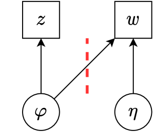
Figure 1: Graphical representation of a two module system with cutting feedback. The dashed line indicates the cut.

There are two data sources, which we denote here as $w$ and $z$. The likelihood term for $z$ depends on $\varphi$, and the likelihood term for $w$ depends on $\eta$ and $\varphi$, and $w$ and $z$ are conditionally independent given $\varphi$. We write $\text{\boldmath$y$}=(\text{\boldmath$w$},\text{\boldmath$z$})$, and set $\text{\boldmath$\theta$}_{1}=\text{\boldmath$\varphi$}$, $\text{\boldmath$\theta$}_{2}=\text{\boldmath$\eta$}$, so that $\text{\boldmath$\theta$}=(\text{\boldmath$\varphi$},\text{\boldmath$\eta$})$. The full posterior density of the joint model can be written in the form (1) as

$$p(\text{\boldmath$\theta$}|\text{\boldmath$y$})\propto p(\text{\boldmath$\theta$})p(\text{\boldmath$y$}|\text{\boldmath$\theta$})=p(\text{\boldmath$\varphi$})p(\text{\boldmath$\eta$}|\text{\boldmath$\varphi$})p(\text{\boldmath$z$}|\text{\boldmath$\varphi$})p(\text{\boldmath$w$}|\text{\boldmath$\varphi$},\text{\boldmath$\eta$}).$$

Figure 1 shows the situation where $p(\text{\boldmath$\eta$}|\text{\boldmath$\varphi$})$ does not depend on $\varphi$, but we allow the more general form of the prior in what follows.

The dashed line in Figure 1 indicates a “cut” in the graph, representing concern that $p(\text{\boldmath$w$}|\text{\boldmath$\varphi$},\text{\boldmath$\eta$})$ may influence inference on $\varphi$. In the modified Gibbs sampling scheme outlined in the previous subsection, the conditional distribution for $\eta$ is unchanged, but the conditional distribution for $\varphi$ is modified to become

$$p_{\text{cut}}(\text{\boldmath$\varphi$}|\text{\boldmath$\eta$},\text{\boldmath$y$})\propto p(\text{\boldmath$\varphi$})p(\text{\boldmath$z$}|\text{\boldmath$\varphi$})\propto p(\text{\boldmath$\varphi$}|\text{\boldmath$z$}).$$

This distribution does not depend on $\eta$, and the modified Gibbs sampler draws independent samples from the cut joint posterior

$$p_{\text{cut}}(\text{\boldmath$\varphi$},\text{\boldmath$\eta$}|\text{\boldmath$y$}) =p(\text{\boldmath$\varphi$}|\text{\boldmath$z$})p(\text{\boldmath$\eta$}|\text{\boldmath$\varphi$},\text{\boldmath$w$}),$$ (2)

where $p(\text{\boldmath$\varphi$}|\text{\boldmath$z$})$ is the marginal posterior density for $\varphi$ given $z$, and $p(\text{\boldmath$\eta$}|\text{\boldmath$\varphi$},\text{\boldmath$w$})$ is the conditional posterior density for $\eta$ given $\text{\boldmath$\varphi$},\text{\boldmath$y$}$ (which does not depend on $z$).

Comparing (2) with the full joint posterior density

$$p(\text{\boldmath$\varphi$},\text{\boldmath$\eta$}|\text{\boldmath$y$}) =p(\text{\boldmath$\varphi$}|\text{\boldmath$y$})p(\text{\boldmath$\eta$}|\text{\boldmath$\varphi$},\text{\boldmath$w$}),$$ (3)

where $p(\text{\boldmath$\varphi$}|\text{\boldmath$y$})$ is the marginal posterior density for $\varphi$ given $y$, we see that in the cut posterior density the term $p(\text{\boldmath$\varphi$}|\text{\boldmath$y$})$ is replaced with $p(\text{\boldmath$\varphi$}|\text{\boldmath$z$})$. Thus in the cut posterior, the model for $w$ does not influence inference about $\varphi$, while uncertainty about $\varphi$ is still propagated when computing inference about $\eta$.

2.4 Applications of cutting feedback

To motivate the importance of the problems we describe it is helpful to discuss some applications of Bayesian modularization and cutting feedback methods. The pharmacokinetic and pharmacodynamic models mentioned in the introduction were some of the first applications, and Lunn et al. (2009) provides a summary. Modularized inference methods have also been widely used in causal inference (McCandless et al., 2010; McCandless et al., 2012; Zigler et al., 2013; Pompe and Jacob, 2021). Propensity scores are a commonly used tool in the causal inference literature, and cut methods can be used to prevent the response model from influencing the estimation of the propensity scores themselves, while still propagating uncertainty about them. Health effects of air pollution are considered in Blangiardo et al. (2011), where they use survey data to adjust ambient pollution level data in describing uncertainty in air pollution exposure. Cut methods can be used here to prevent a possibly misspecified module for health outcomes from influencing exposure estimates. Nicholson et al. (2021) consider the notion of “interoperability” in modelling for pandemic preparedness, which incorporates modularity as one key statistical principle.

Two-stage estimation methods are widely used in econometric analysis, where auxiliary models are used to impute observed values in the response model. These methods are closely related to cutting feedback approaches in the Bayesian context. In two-stage methods, accurate propagation of uncertainty in the imputed values is important when undertaking inference; see Murphy and Topel (2002). A key application is endogeneity correction, which is necessary in many social science studies; for example, in marketing (Petrin and Train, 2010).

Liu et al. (2009) were motivated to study modularized Bayesian methods by applications to the analysis of computer models. They consider other applications as well, such as meta-analysis, and this is also considered for a problem in ecology by Ogle et al. (2013). A semi-modular approach to geographically weighted regression has been recently discussed in Liu and Goudie (2021), where choosing how much to pool information spatially in a local estimation procedure can be thought of as a problem of managing model misspecification. An interesting archaeological application for cut methods, where one of the modules involves only prior terms, is discussed by Styring et al. (2017) and Carmona and Nicholls (2020), and we discuss this later. Similar to Styring et al. (2017), Moss and Rousseau (2022) also consider cut methods for priors but in the context of hidden Markov models.

The references we have given here about modularized inference applications are not exhaustive, and each of them is often typical of a larger body of work in a certain discipline.

3 Mean field variational inference for cut models

In this Section we describe variational inference methods for defining cut posterior distributions based on mean field approximations and variational message passing algorithms. These methods are analogous to the implicit definitions of a cut posterior distribution considered in Section 2.1 based on modified Gibbs sampling algorithms. There is previous work on variational inference with misspecification (Wang and Blei, 2019) as well as for so-called Gibbs posterior distributions (Alquier et al., 2016; Frazier et al., 2021), but variational inference for modularized anlayses are different in the sense that a full probabilistic model is assumed, but serious misspecification is confined to only some model components.

3.1 Variational inference

Variational approximations of a Bayesian posterior distribution are obtained by minimization of a divergence measure between an approximating density and the true posterior density $p(\text{\boldmath$\theta$}|\text{\boldmath$y$})\propto p(\text{\boldmath$\theta$})p(\text{\boldmath$y$}|\text{\boldmath$\theta$})$. The Kullback-Leibler divergence is the most popular metric adopted, so that for an approximating family ${\cal F}$ of densities, the optimal approximating density is

$$q^{*}(\text{\boldmath$\theta$}) =\arg\min_{q(\text{\boldmath$\theta$})\in{\cal F}}\text{KL}(q(\text{\boldmath$\theta$})||p(\text{\boldmath$\theta$}|\text{\boldmath$y$})),$$ (4)

where

$$\text{KL}(q(\text{\boldmath$\theta$})||p(\text{\boldmath$\theta$}|\text{\boldmath$y$})) =\int\log\frac{q(\text{\boldmath$\theta$})}{p(\text{\boldmath$\theta$}|\text{\boldmath$y$})}q(\text{\boldmath$\theta$})\,d\text{\boldmath$\theta$}$$ (5)

is the Kullback-Leibler divergence between $q(\text{\boldmath$\theta$})$ and $p(\text{\boldmath$\theta$}|\text{\boldmath$y$})$. It is straightforward to show that the optimization at (4) is equivalent to

$$q^{*}(\text{\boldmath$\theta$}) =\arg\max_{q(\text{\boldmath$\theta$})\in{\cal F}}{\cal L}(q),$$ (6)

where ${\cal L}(q)$ is called the evidence lower bound (ELBO), and defined as

$${\cal L}(q) =\int\log\frac{p(\text{\boldmath$\theta$})p(\text{\boldmath$y$}|\text{\boldmath$\theta$})}{q(\text{\boldmath$\theta$})}q(\text{\boldmath$\theta$})d\text{\boldmath$\theta$}.$$ (7)

Overviews of variational inference are given in Ormerod and Wand (2010) and Blei et al. (2017). The approximating family ${\cal F}$ is usually defined by either a product restriction (leading to mean field approximations) or fixed form approximations. We consider mean field approximations first.

3.2 Mean field approximations and variational message passing

Similar to Section 2.1, let $\text{\boldmath$\theta$}=(\text{\boldmath$\theta$}_{1}^{\top},\dots,\text{\boldmath$\theta$}_{K}^{\top})^{\top}$ be a partition of $\theta$ into $K$ blocks, and suppose ${\cal F}$ consists of densities that have the form

$$q(\text{\boldmath$\theta$}) =\prod_{i=1}^{K}q_{i}(\text{\boldmath$\theta$}_{i}).$$ (8)

Considering the $i$th term $q_{i}(\text{\boldmath$\theta$}_{i})$ in (8) and with the terms $q_{j}(\text{\boldmath$\theta$}_{j})$, $j\neq i$ held fixed, the value for $q_{i}(\text{\boldmath$\theta$}_{i})$ solving the optimization problem at (6) is

$$q_{i}^{*}(\text{\boldmath$\theta$}_{i}) \propto\exp\left(E_{-\text{\boldmath$\theta$}_{i}}(\log p(\text{\boldmath$\theta$})p(\text{\boldmath$y$}|\text{\boldmath$\theta$}))\right),$$ (9)

where $E_{-\text{\boldmath$\theta$}_{i}}(\cdot)$ denotes expectation with respect to the density $\prod_{j\neq i}q_{j}(\text{\boldmath$\theta$}_{j})$ (see, for example, Ormerod and Wand (2010)). The update (9) can be used in a coordinate ascent optimization scheme, where after initialization we cycle through the terms in $q(\text{\boldmath$\theta$})$, updating each using (9) until convergence. We can also write (9) as

$$q^{*}_{i}(\text{\boldmath$\theta$}_{i}) \propto\exp\left(E_{-\text{\boldmath$\theta$}_{i}}(\log p(\text{\boldmath$\theta$}_{i}|\text{\boldmath$\theta$}_{-i},\text{\boldmath$y$}))\right),$$ (10)

where $p(\text{\boldmath$\theta$}_{i}|\text{\boldmath$\theta$}_{-i},\text{\boldmath$y$})$ is the posterior full conditional distribution for $\text{\boldmath$\theta$}_{i}$, and this formulation shows the close connection between mean field variational inference and Gibbs sampling.

Consider the factorization of the joint model (1). Then

$$\log p(\text{\boldmath$\theta$})p(\text{\boldmath$y$}|\text{\boldmath$\theta$}) =\sum_{j=1}^{M}\log f_{j}(\text{\boldmath$\theta$}_{A(j)}),$$

and the update (9) can be written as

$$q^{*}_{i}(\text{\boldmath$\theta$}_{i}) \propto\prod_{j:i\in A(j)}m_{f_{j}\rightarrow\text{\boldmath$\theta$}_{i}}(\text{\boldmath$\theta$}_{i}),$$ (11)

where

$$m_{f_{j}\rightarrow\text{\boldmath$\theta$}_{i}}(\text{\boldmath$\theta$}_{i}) =\exp\left(E_{-\text{\boldmath$\theta$}_{i}}(\log f_{j}(\text{\boldmath$\theta$}_{A(j)}))\right).$$

The functions $m_{f_{j}\rightarrow\text{\boldmath$\theta$}_{i}}(\text{\boldmath$\theta$}_{i})$ may be thought of as “messages” from factor $f_{j}(\cdot)$ in the model to $\text{\boldmath$\theta$}_{i}$. For more general discussions of variational message passing algorithms, see Winn and Bishop (2005), Minka (2005), Knowles and Minka (2011) and Wand (2017). Wand (2017) considers a message passing formulation of mean field approximations involving messages from both model factors to parameters and factors to parameters, representing the model using a factor graph. Computations are formulated in terms of factor graph fragments, and the approach ensures computational modularity and allows extensions to arbitrarily large models.

3.3 Cutting feedback with message passing

The factorization of the update (9) into a product of messages motivates one approach to defining a cut variational posterior distribution. Write $q^{*}_{1}(\text{\boldmath$\theta$}_{1}),\dots,q^{*}_{K}(\text{\boldmath$\theta$}_{K})$ for the terms of the mean field approximation optimizing the ELBO without cutting feedback. Similar to the discussion of modified Gibbs sampling algorithms in Section 2, suppose that factor $f_{k}(\text{\boldmath$\theta$}_{A(k)})$ in the joint model is thought to be misspecified, and that we are concerned about the effect of this misspecification on $\text{\boldmath$\theta$}_{1}$. We can construct a cut marginal posterior distribution for $\text{\boldmath$\theta$}_{1}$ by changing $q^{*}_{1}(\text{\boldmath$\theta$}_{1})$ to

$$q_{\text{cut},1}(\text{\boldmath$\theta$}_{1}) \propto\prod_{j:1\in A(j),j\neq k}m_{f_{j}\rightarrow\text{\boldmath$\theta$}_{1}}(\text{\boldmath$\theta$}_{1}).$$ (12)

where the messages in (12) are the ones obtained at convergence in approximating the true posterior, but the message from factor $f_{k}(\cdot)$ to $\text{\boldmath$\theta$}_{1}$ is left out. After defining a cut marginal posterior distribution for $\text{\boldmath$\theta$}_{1}$ in this way, we then fix $q_{1}(\text{\boldmath$\theta$}_{1})$ to (12) and optimize the remaining terms $q_{2}(\text{\boldmath$\theta$}_{2}),\dots,q_{K}(\text{\boldmath$\theta$}_{K})$ using the usual update (9) until convergence, resulting in optimal terms $q_{\text{cut},i}(\text{\boldmath$\theta$}_{i})$, $i=2,\dots,K$. The variational cut posterior is then

$$q_{\text{cut}}(\text{\boldmath$\theta$}) =\prod_{i=1}^{K}q_{\text{cut},i}(\text{\boldmath$\theta$}_{i}),$$ (13)

and is an approximation to the joint posterior maximizing the ELBO subject to constraining the $\text{\boldmath$\theta$}_{1}$ marginal to be (12). Other modifications of variational message passing algorithms can also be used to produce cut procedures and posteriors. Algorithm 1 describes explicitly cut variational message passing for a single cut of the model factor $f_{k}(\cdot)$ on $\text{\boldmath$\theta$}_{1}$.

Algorithm 1 Cut variational posterior via message passing: removing the contribution of $f_{k}(\cdot)$ to $\theta_{1}$.

Initialization:

• Initialize $q_{2}(\text{\boldmath$\theta$}_{2}),\dots,q_{K}(\text{\boldmath$\theta$}_{K})$.

Computation of cut posterior density $\prod_{i=1}^{K}q_{\text{cut},i}(\text{\boldmath$\theta$}_{i})$:

1. Until convergence do:

   • For $i=1,\dots,K$:
     

     $$q_{i}(\text{\boldmath$\theta$}_{i})\leftarrow C_{i}(q)^{-1}\left\{\prod_{j:i\in A(j)}m_{f_{j}\rightarrow\text{\boldmath$\theta$}_{i}}(\text{\boldmath$\theta$}_{i})\right\},$$

     where $C_{i}(q)$ is a normalizing constant making $q_{i}(\text{\boldmath$\theta$}_{i})$ integrate to one. $C_{i}(q)$ will depend on the factor $i$ being updated and the current value of $q$.

2. Calculate

   $$q_{\text{cut},1}(\text{\boldmath$\theta$}_{1})=C_{\text{cut},1}^{-1}\prod_{j:1\in A(j),j\neq k}m_{f_{j}\rightarrow\text{\boldmath$\theta$}_{1}}(\text{\boldmath$\theta$}_{1}),$$

   where $C_{\text{cut},1}$ is a normalizing constant making $q_{\text{cut},1}(\text{\boldmath$\theta$}_{1})$ integrate to one.

3. For $i=2,\dots,K$, initialize $q_{\text{cut},i}(\text{\boldmath$\theta$}_{i})=q_{i}(\text{\boldmath$\theta$}_{i})$.

4. Until convergence do:

   • For $i=2,\dots,K$:
     

     $$q_{\text{cut},i}(\text{\boldmath$\theta$}_{i})\leftarrow C_{i}(q_{\text{cut}})^{-1}\left\{\prod_{j:i\in A(j)}m_{f_{j}\rightarrow\text{\boldmath$\theta$}_{i}}^{\text{cut}}(\text{\boldmath$\theta$}_{i})\right\},$$

     where $C_{i}(q_{\text{cut}})$ is a normalizing constant making $q_{\text{cut},i}(\text{\boldmath$\theta$}_{i})$ integrate to one, and

     $$m_{f_{j}\rightarrow\text{\boldmath$\theta$}_{i}}^{\text{cut}}(\text{\boldmath$\theta$}_{i})=\exp\left(E_{-\text{\boldmath$\theta$}_{i}}^{\text{cut}}(\log f_{j}(\theta_{A(j)}))\right),$$

     where $E_{-\text{\boldmath$\theta$}_{i}}^{\text{cut}}(\cdot)$ denotes expectation with respect to $\prod_{l\neq i}q_{\text{cut},l}(\text{\boldmath$\theta$}_{l})$.

5. Return $q_{\text{cut}}(\text{\boldmath$\theta$})=\prod_{i=1}^{K}q_{\text{cut},i}(\text{\boldmath$\theta$}_{i})$.

We call the variational message passing approach to evaluating the cut posterior “cut variational message passing”, and now elaborate further on its use in the two module system of Figure 1. Suppose we use a factorized variational approximation,

$$q(\text{\boldmath$\theta$})=q_{\text{\boldmath$\varphi$}}(\text{\boldmath$\varphi$})q_{\text{\boldmath$\eta$}}(\text{\boldmath$\eta$}).$$

The coordinate ascent update for $q_{\text{\boldmath$\varphi$}}(\text{\boldmath$\varphi$})$ is a product of three messages,

$$q_{\text{\boldmath$\varphi$}}^{*}(\text{\boldmath$\varphi$})\propto m_{p(\text{\boldmath$\varphi$})\rightarrow\text{\boldmath$\varphi$}}(\text{\boldmath$\varphi$})\times m_{p(\text{\boldmath$z$}|\text{\boldmath$\varphi$})\rightarrow\text{\boldmath$\varphi$}}(\text{\boldmath$\varphi$})\times m_{p(\text{\boldmath$w$}|\text{\boldmath$\varphi$},\text{\boldmath$\eta$})\rightarrow\text{\boldmath$\varphi$}}(\text{\boldmath$\varphi$}).$$

It is easy to see from our definition of the messages that $m_{p(\text{\boldmath$\varphi$})\rightarrow\text{\boldmath$\varphi$}}(\text{\boldmath$\varphi$})=p(\text{\boldmath$\varphi$})$ and $m_{p(\text{\boldmath$z$}|\text{\boldmath$\varphi$})\rightarrow\text{\boldmath$\varphi$}}(\text{\boldmath$\varphi$})=p(\text{\boldmath$z$}|\text{\boldmath$\varphi$})$, regardless of what $q_{\text{\boldmath$\eta$}}(\text{\boldmath$\eta$})$ is. Hence when we cut, the variational cut marginal for $\varphi$ is

$$q_{\text{cut},\text{\boldmath$\varphi$}}(\text{\boldmath$\varphi$})\propto p(\text{\boldmath$\varphi$})p(\text{\boldmath$z$}|\text{\boldmath$\varphi$}),$$

and hence $q_{\text{cut},\text{\boldmath$\varphi$}}(\text{\boldmath$\varphi$})$ is the exact cut posterior for $\varphi$. Once the cut marginal for $\varphi$ is fixed in this way, iteration is not required to find the remaining factor $q_{\text{cut},\text{\boldmath$\eta$}}(\text{\boldmath$\eta$})$, which is given by the update (9).

For non-conjugate models, message passing methods can be difficult to employ because the messages involve expectations that cannot be expressed in closed form and are difficult to compute. In this case, methods such as nonconjugate variational message passing (NCVMP) (Knowles and Minka, 2011) and Monte Carlo coordinate ascent variational inference (MC-CAVI) (Ye et al., 2020) can be used. However, we instead use methods based on black box variational inference and fixed form approximations described in Section 4.

3.4 Illustrative example revisited

To illustrate the cut posterior distribution based on variational message passing, we return to the biased data example in Section 2.1. We compare four distributions: the full posterior, cut posterior, and variational approximations to both. The exact cut posterior distribution has the density at (2), which incorporates the cut of the two module structure depicted in Figure 1. Both the full posterior density and cut posterior density are multivariate normal, and can be computed analytically.

The coordinate ascent updates for $q_{\varphi}(\varphi)$ and $q_{\eta}(\eta)$ at (11) are

$$q^{*}_{\varphi}(\varphi) \propto m_{p(\varphi)\rightarrow\varphi}(\varphi)\times m_{p(\text{\boldmath$z$}|\varphi)\rightarrow\varphi}(\varphi)\times m_{p(\text{\boldmath$w$}|\varphi,\eta)\rightarrow\varphi}(\varphi),$$

$$q^{*}_{\eta}(\eta) \propto m_{p(\eta)\rightarrow\eta}(\eta)\times m_{p(\text{\boldmath$w$}|\varphi,\eta)\rightarrow\eta}(\eta).$$

The expectations required to compute the messages above can be evaluated in closed form, as outlined in Appendix A. To specify the variational posterior for $\varphi$, we use the full variational marginal posterior at convergence $q^{*}_{\varphi}(\varphi)$ but remove the message $m_{p(\text{\boldmath$w$}|\varphi,\eta)\rightarrow\varphi}(\varphi)$ to get the variational cut marginal density for $\varphi$, denoted $q_{\text{cut},\varphi}(\varphi)$. Then we perform a single update for $q_{\eta}(\eta)$ to obtain its optimal value with $q_{\varphi}(\varphi)$ fixed at $q_{\text{cut},\varphi}(\varphi)$ to obtain the cut variational marginal for $\eta$, denoted as $q_{\text{cut},\eta}(\eta)$. Therefore, the final variational cut joint posterior is $q_{\text{cut}}(\varphi,\eta)=q_{\text{cut},\varphi}(\varphi)q_{\text{cut},\eta}(\eta)$.

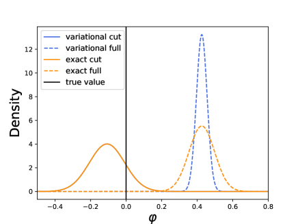
(a) Exact (orange) and variational (blue) cut and full posterior densities of $\varphi$. The variational cut and exact cut posterior densities coincide.

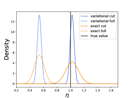
(b) Exact (orange) and variational (blue) cut and full posterior densities of $\eta$.

Figure 2: Comparison of marginal posterior estimates of $\varphi$ (left) and $\eta$ (right).

Figure 2 shows the marginal posterior densities for the exact full posterior (dashed orange), the exact cut posterior (solid orange), the variational full posterior (dashed blue), the variational cut posterior (solid blue) and the true values (vertical black lines). We make four observations. First, for parameter $\varphi$ the variational and exact cut posterior are the same in this example, which is expected following the discussion in Section 3.3. Second, for both $\varphi$ and $\eta$, the full posteriors (whether exact or variational) provide poor inference, in the sense that the true values $\varphi=0$ and $\eta=1$ lie out in the tails of these distributions. The misspecification in the biased data module has contaminated the inference for the full posterior and its variational approximation. Third, for both exact and variational cut posteriors, cutting feedback has mitigated the problem of contamination. For the cut distributions the true parameter values are in the high probability regions. Fourth, the variational distributions underestimate uncertainty compared to their exact counterparts.

The cause of the underestimation of uncertainty for the variational methods is the lack of flexibility of the factorized form of the mean field approximation. This is shown in the comparison of the joint posterior distributions for $(\varphi,\eta)$ for the exact and variational posterior distributions in Figure 3. The variational approximations assume independence between $\varphi$ and $\eta$. Expressions for the exact posterior density, exact cut posterior density and variational cut posterior density are given in Appendix A. The expression for the variational cut posterior marginal for $\eta$ shows that it is obtained as the full conditional density for $\eta$ conditioned on a certain point estimate for $\varphi$. This gives an intuitive interpretation of the underestimation of uncertainty in this marginal density due to ignoring propagation of uncertainty. The fixed form variational approximations used in the next section address some of the problems of mean field approximations by allowing greater flexibility for capturing the dependence structure.

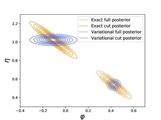
Figure 3: Contour plots of joint posterior distributions for biased data example. The variational approximations employ a mean field assumption.

4 Defining the cut posterior through optimization

In this section we consider the two module system depicted in Figure 1. We first highlight why it can be difficult to use MCMC methods to sample directly from the cut posterior of this system at (2). However, we then show that the cut posterior can be formulated as the solution to a constrained optimization problem, which is attractive from an optimization-based perspective on Bayesian inference (Knoblauch et al., 2019). Finally, motivated by this observation, we propose fixed form variational approximations that can be used to compute inference in a computationally attractive fashion. In concurrent independent work Carmona and Nicholls (2022) have also considered variational inference methods in modularized Bayesian analyses, and they consider normalizing flows for constructing flexible posterior approximations. However, the focus of their work is on semi-modular inference (Carmona and Nicholls, 2020) rather than cutting feedback.

4.1 The cut posterior

The cut posterior density at (2) can be expressed as

$$p_{\text{cut}}(\text{\boldmath$\varphi$},\text{\boldmath$\eta$}|\text{\boldmath$y$}) =p(\text{\boldmath$\varphi$}|\text{\boldmath$z$})p(\text{\boldmath$\eta$}|\text{\boldmath$\varphi$},\text{\boldmath$y$})$$

$$\propto p(\text{\boldmath$\varphi$})p(\text{\boldmath$z$}|\text{\boldmath$\varphi$})\frac{p(\text{\boldmath$\eta$}|\text{\boldmath$\varphi$})p(\text{\boldmath$y$}|\text{\boldmath$\eta$},\text{\boldmath$\varphi$})}{p(\text{\boldmath$y$}|\text{\boldmath$\varphi$})}$$

$$=p(\text{\boldmath$\varphi$})p(\text{\boldmath$z$}|\text{\boldmath$\varphi$})\frac{p(\text{\boldmath$\eta$}|\text{\boldmath$\varphi$})p(\text{\boldmath$w$}|\text{\boldmath$\eta$},\text{\boldmath$\varphi$})}{p(\text{\boldmath$w$}|\text{\boldmath$\varphi$})},$$ (14)

where we can obtain the last line from the previous one by observing that $p(\text{\boldmath$\eta$}|\text{\boldmath$\varphi$},\text{\boldmath$y$})=p(\text{\boldmath$\eta$}|\text{\boldmath$\varphi$},\text{\boldmath$w$})$ and using the definition of these conditional densities.

Sampling from this posterior distribution using MCMC is difficult, because of the marginal likelihood term $p(\text{\boldmath$w$}|\text{\boldmath$\varphi$})$ that appears on the right-hand side of (14), which is often intractable. Current suggestions in the literature to sample from the cut posterior are computationally intensive and may not sample exactly from the correct target. Plummer (2015) observes that the cut posterior is often defined only implicitly through modification of an MCMC sampling scheme, and that the implied posterior density differs according to the proposal used in Metropolis-within-Gibbs schemes. The same difficulty has also been pointed out in Woodard et al. (2013). Plummer (2015) suggests to use current cut software implementations with caution and performing appropriate sensitivity analyses. He outlines computationally intensive multiple imputation (Little, 1992) and tempered MCMC approaches to sampling. Some advanced MCMC methods for sampling the cut posterior have been considered recently in Jacob et al. (2020) and Liu and Goudie (2020). Pompe and Jacob (2021) consider a posterior bootstrap approach to cut model computation having frequentist validity, and they develop some asymptotic theory for cut posteriors. Frazier and Nott (2022) study theoretically the behaviour of cut conditional posterior distributions, which is useful for understanding how uncertainty propagates between modules. Their normal approximations of conditional cut posterior densities are useful for both computation and diagnostic purposes.

We now demonstrate that the cut posterior can be formulated as the solution to a constrained optimization problem, which leads to variational computational methods. Let $q_{\varphi}(\text{\boldmath$\varphi$})=\int q(\text{\boldmath$\varphi$},\text{\boldmath$\eta$})\mbox{d}\text{\boldmath$\eta$}$ be the marginal density in $\varphi$ of the approximating density $q(\text{\boldmath$\varphi$},\text{\boldmath$\eta$})$. Then define the family of densities

$${\cal F}_{\text{cut}}=\{q(\text{\boldmath$\varphi$},\text{\boldmath$\eta$}):q_{\varphi}(\text{\boldmath$\varphi$})=p(\text{\boldmath$\varphi$}|\text{\boldmath$z$})\}.$$

${\cal F}_{\text{cut}}$ is the family of approximations preserving the exact cut posterior marginal in $\varphi$. The following lemma shows that the density in ${\cal F}_{\text{cut}}$ that is the best approximation to the full (i.e. uncut) posterior density in the Kullback-Leibler sense, is given by $p_{\text{cut}}(\text{\boldmath$\eta$},\text{\boldmath$\varphi$}|\text{\boldmath$y$})$ at (2). Part (b) of the lemma states a result which is used further below: it demonstrates that the KL divergence between the cut and full posterior is the KL divergence between their $\varphi$ marginals. This result will be useful later when we develop diagnostic methods for deciding whether or not to cut.

Lemma 1.

With ${\cal F}_{\text{cut}}$ as defined above,

• $p_{\text{cut}}(\text{\boldmath$\varphi$},\text{\boldmath$\eta$}|\text{\boldmath$y$})=\arg\min_{q\in{\cal F}_{\text{cut}}}\text{KL}(q(\text{\boldmath$\varphi$},\text{\boldmath$\eta$})||p(\text{\boldmath$\varphi$},\text{\boldmath$\eta$}|\text{\boldmath$y$})).$

• $\text{KL}(p(\text{\boldmath$\varphi$},\text{\boldmath$\eta$}|\text{\boldmath$y$})||p_{\text{cut}}(\text{\boldmath$\varphi$},\text{\boldmath$\eta$}|\text{\boldmath$y$}))=\text{KL}(p(\text{\boldmath$\varphi$}|\text{\boldmath$y$})||p(\text{\boldmath$\varphi$}|\text{\boldmath$z$})).$

Proof.

Write $q(\text{\boldmath$\varphi$},\text{\boldmath$\eta$})\in{\cal F}_{\text{cut}}$ as $q(\text{\boldmath$\varphi$},\text{\boldmath$\eta$})=p(\text{\boldmath$\varphi$}|\text{\boldmath$z$})q(\text{\boldmath$\eta$}|\text{\boldmath$\varphi$})$, and $E_{q}(\cdot)$ for the expectation with respect to $q(\text{\boldmath$\varphi$},\text{\boldmath$\eta$})$. Since

$$\log\frac{q(\text{\boldmath$\varphi$},\text{\boldmath$\eta$})}{p(\text{\boldmath$\varphi$},\text{\boldmath$\eta$}|\text{\boldmath$y$})} =\log\frac{p(\text{\boldmath$\varphi$}|\text{\boldmath$z$})q(\text{\boldmath$\eta$}|\text{\boldmath$\varphi$})}{p(\text{\boldmath$\varphi$}|\text{\boldmath$y$})p(\text{\boldmath$\eta$}|\text{\boldmath$\varphi$},\text{\boldmath$w$})}$$

$$=\log\frac{p(\text{\boldmath$\varphi$}|\text{\boldmath$z$})}{p(\text{\boldmath$\varphi$}|\text{\boldmath$y$})}+\log\frac{q(\text{\boldmath$\eta$}|\text{\boldmath$\varphi$})}{p(\text{\boldmath$\eta$}|\text{\boldmath$\varphi$},\text{\boldmath$w$})},$$

we have

$$\text{KL}(q(\text{\boldmath$\varphi$},\text{\boldmath$\eta$})||p(\text{\boldmath$\varphi$},\text{\boldmath$\eta$}|\text{\boldmath$y$})) =E_{q}\left(\log\frac{q(\text{\boldmath$\varphi$},\text{\boldmath$\eta$})}{p(\text{\boldmath$\varphi$},\text{\boldmath$\eta$}|\text{\boldmath$y$})}\right)$$

$$=E_{q}\left(\log\frac{p(\text{\boldmath$\varphi$}|\text{\boldmath$z$})}{p(\text{\boldmath$\varphi$}|\text{\boldmath$y$})}\right)+E_{q}\left(\log\frac{q(\text{\boldmath$\eta$}|\text{\boldmath$\varphi$})}{p(\text{\boldmath$\eta$}|\text{\boldmath$\varphi$},\text{\boldmath$w$})}\right).$$ (15)

The first term on the right-hand side of (15) does not depend on $q(\text{\boldmath$\varphi$},\text{\boldmath$\eta$})$. Hence the $q(\text{\boldmath$\varphi$},\text{\boldmath$\eta$})$ minimizing the above expression minimizes the second term,

$$E_{q}\left(\log\frac{q(\text{\boldmath$\eta$}|\text{\boldmath$\varphi$})}{p(\text{\boldmath$\eta$}|\text{\boldmath$\varphi$},\text{\boldmath$w$})}\right) =\int\int\log\frac{q(\text{\boldmath$\eta$}|\text{\boldmath$\varphi$})}{p(\text{\boldmath$\eta$}|\text{\boldmath$\varphi$},\text{\boldmath$w$})}q(\text{\boldmath$\eta$}|\text{\boldmath$\varphi$})d\text{\boldmath$\eta$}\,d\text{\boldmath$\varphi$}.$$ (16)

The inner integral on the right-hand side of (16) is the KL-divergence between $q(\text{\boldmath$\eta$}|\text{\boldmath$\varphi$})$ and $p(\text{\boldmath$\eta$}|\text{\boldmath$\varphi$},\text{\boldmath$w$})$. The integral attains the minimum possible value of zero if we choose, for every $\varphi$, $q(\text{\boldmath$\eta$}|\text{\boldmath$\varphi$})=p(\text{\boldmath$\eta$}|\text{\boldmath$\varphi$},\text{\boldmath$w$})$. This choice corresponds to the cut posterior distribution. This establishes part (a) of the lemma.

Similar to the above argument, we can write $\text{KL}(p(\text{\boldmath$\varphi$},\text{\boldmath$\eta$}|\text{\boldmath$y$})||p_{\text{cut}}(\text{\boldmath$\varphi$},\text{\boldmath$\eta$}|\text{\boldmath$y$}))$ as the sum of $\text{KL}(p(\text{\boldmath$\varphi$}|\text{\boldmath$y$})||p(\text{\boldmath$\varphi$}|\text{\boldmath$z$}))$ and the expectation with respect to $p(\text{\boldmath$\varphi$}|\text{\boldmath$y$})$ of $\text{KL}(p(\text{\boldmath$\eta$}|\text{\boldmath$\varphi$},\text{\boldmath$w$})||p_{\text{cut}}(\text{\boldmath$\eta$}|\text{\boldmath$\varphi$},\text{\boldmath$w$}))$, with the latter term being zero, which proves (b). ∎

4.2 Fixed form approximations

Lemma 1 motivates a simple variational approach to approximating the cut posterior. It employs a variational family of fixed form approximations with a finite set of parameters called “variational parameters”.

Consider an approximation to $p(\text{\boldmath$\varphi$}|\text{\boldmath$z$})$ of the form $q_{\widetilde{\lambda}}(\text{\boldmath$\varphi$})$, with parameters $\widetilde{\text{\boldmath$\lambda$}}$. The most accurate approximation in this family (in the Kullback-Leibler sense) has parameter values

$$\widetilde{\text{\boldmath$\lambda$}}^{*}=\arg\max_{\widetilde{\text{\boldmath$\lambda$}}}\int\log\frac{p(\text{\boldmath$\varphi$})p(\text{\boldmath$z$}|\text{\boldmath$\varphi$})}{q_{\widetilde{\lambda}}(\text{\boldmath$\varphi$})}q_{\widetilde{\lambda}}(\text{\boldmath$\varphi$})d\text{\boldmath$\varphi$}.$$

Solving a variational optimization targeting the exact cut marginal posterior for $\varphi$ ensures that the second module data cannot influence the variational cut marginal posterior density for $\varphi$.

Writing $\text{\boldmath$\lambda$}=(\widetilde{\text{\boldmath$\lambda$}}^{\top},\breve{\text{\boldmath$\lambda$}}^{\top})^{\top}$, we can then approximate the optimization over ${\cal F}_{\text{cut}}$ in part (a) of Lemma 1 by an optimization over the family

$$\widetilde{{\cal F}}_{\text{cut}}=\{q_{\lambda}(\text{\boldmath$\varphi$},\text{\boldmath$\eta$}):q_{\lambda}(\text{\boldmath$\varphi$},\text{\boldmath$\eta$})=q_{\widetilde{\lambda}^{*}}(\text{\boldmath$\varphi$})q_{\breve{\lambda}}(\text{\boldmath$\eta$}|\text{\boldmath$\varphi$})\},$$

where the fixed marginal $q_{\widetilde{\lambda}^{*}}(\text{\boldmath$\varphi$})$ from the first stage optimization approximates $p(\text{\boldmath$\varphi$}|\text{\boldmath$z$})$, and we have approximated the conditional posterior distribution for $\eta$ given $\varphi$ by some parametric form $q_{\breve{\lambda}}(\text{\boldmath$\eta$}|\text{\boldmath$\varphi$})$ with variational parameters $\breve{\text{\boldmath$\lambda$}}$. The optimization in part (a) of Lemma 1 is an optimization targeting the full posterior distribution, so there is no need to compute the intractable term $p(\text{\boldmath$w$}|\text{\boldmath$\varphi$})$ in (14). It is an ordinary variational optimization, where the approximation to the cut posterior distribution arises from the choice of the variational family and not through changing the target for the approximation. Finally, defining

$$\breve{\text{\boldmath$\lambda$}}^{*}=\arg\max_{\breve{\text{\boldmath$\lambda$}}}\int\log\frac{p(\text{\boldmath$\varphi$})p(\text{\boldmath$\eta$}|\text{\boldmath$\varphi$})p(\text{\boldmath$z$}|\text{\boldmath$\varphi$})p(\text{\boldmath$w$}|\text{\boldmath$\varphi$},\text{\boldmath$\eta$})}{q_{\widetilde{\lambda}^{*}}(\text{\boldmath$\varphi$})q_{\breve{\lambda}}(\text{\boldmath$\eta$}|\text{\boldmath$\varphi$})}q_{\widetilde{\lambda}^{*}}(\text{\boldmath$\varphi$})q_{\breve{\lambda}}(\text{\boldmath$\eta$}|\text{\boldmath$\varphi$})\,d\text{\boldmath$\varphi$}d\text{\boldmath$\eta$},$$

gives an approximation $q_{\lambda^{*}}(\text{\boldmath$\varphi$},\text{\boldmath$\eta$})=q_{\widetilde{\lambda}^{*}}(\text{\boldmath$\varphi$})q_{\breve{\lambda}^{*}}(\text{\boldmath$\eta$}|\text{\boldmath$\varphi$})$ to (2) with calibrated variational parameters $\text{\boldmath$\lambda$}^{*}=((\widetilde{\text{\boldmath$\lambda$}}^{*})^{\top},(\breve{\text{\boldmath$\lambda$}}^{*})^{\top})^{\top}$. $\breve{\text{\boldmath$\lambda$}}^{*}$ has the interpretation of minimizing the KL divergence of the approximation to the full posterior distribution within the family $\widetilde{{\cal F}}_{\text{cut}}$.

There is another way of viewing the two-stage optimization procedure above, which was recently discussed in Carmona and Nicholls (2022). The authors show that the minimum KL divergence between a given density $q_{\widetilde{\lambda}}(\text{\boldmath$\varphi$})q_{\breve{\lambda}}(\text{\boldmath$\eta$}|\text{\boldmath$\varphi$})$ and the densities in ${\cal F}_{\text{cut}}$ is $\text{KL}(q_{\widetilde{\lambda}}(\text{\boldmath$\varphi$})||p(\text{\boldmath$\varphi$}|\text{\boldmath$z$}))$, with this not depending on $\breve{\text{\boldmath$\lambda$}}$. This formulates the first stage of the optimization in our approach in a similar way to the second, as an optimization over a family of joint densities for $(\text{\boldmath$\varphi$},\text{\boldmath$\eta$})$. This allows the entire two stage procedure to be seen as optimizing a well-defined objective function (Carmona and Nicholls (2022), Proposition 9) by considering a certain family of variational objectives indexed by a hyperparameter, and taking the hyperparameter to a limit. The results of Carmona and Nicholls (2022) are in the context of semi-modular inference, with cutting feedback as a special case.

While there is a wide range of fixed form densities that can be used for the variational family, a popular choice for continuous-valued $\text{\boldmath$\theta$}=(\text{\boldmath$\varphi$}^{\top},\text{\boldmath$\eta$}^{\top})^{\top}$ is to assume

$$q_{\lambda}(\text{\boldmath$\varphi$},\text{\boldmath$\eta$}) =q_{\widetilde{\lambda}}(\text{\boldmath$\varphi$})q_{\breve{\lambda}}(\text{\boldmath$\eta$}|\text{\boldmath$\varphi$})$$

is the density of a $N(\text{\boldmath$\mu$},\bm{\Sigma})$ distribution. If some parameters are constrained, then they can be transformed to the real line so that they have the same support as the approximation. Set $\bm{\Sigma}=\bm{C}\bm{C}^{\top}$, where $\bm{C}$ is the lower-triangular Cholesky factor, and partition $\mu$ and $\bm{C}$ to conform with $\theta$, so that $\text{\boldmath$\mu$}=(\text{\boldmath$\mu$}_{\varphi}^{\top},\text{\boldmath$\mu$}_{\eta}^{\top})^{\top}$, and

$$\bm{C}=\left[\begin{array}[]{cc}\bm{C}_{\varphi}&\bm{0}\\ \bm{C}_{\varphi\eta}&\bm{C}_{\eta}\end{array}\right],$$

where $\bm{C}_{\varphi}$ and $\bm{C}_{\eta}$ are both lower triangular. Here $\widetilde{\text{\boldmath$\lambda$}}=(\text{\boldmath$\mu$}_{\varphi}^{\top},\text{vech}(\bm{C}_{\varphi})^{\top})^{\top}$, where vech is the half-vectorization operator which stacks the lower-triangular elements of a matrix column-by-column, and $\breve{\text{\boldmath$\lambda$}}=(\text{\boldmath$\mu$}_{\eta}^{\top},\text{vec}(\bm{C}_{\varphi\eta})^{\top},\text{vech}(\bm{C}_{\eta})^{\top})^{\top},$ where vec is the vectorization operator. Optimization of a Gaussian variational approximation parametrized by its mean vector and lower-triangular Cholesky factor of its covariance matrix via stochastic gradient methods is considered by Titsias and Lázaro-Gredilla (2014) and Kucukelbir et al. (2017) among others. For the second-stage optimization it is straightforward to simply fix the variational parameters $\widetilde{\text{\boldmath$\lambda$}}=\widetilde{\text{\boldmath$\lambda$}}^{*}$ and only optimize over $\breve{\text{\boldmath$\lambda$}}$. We do not discuss implementation details of methods for lower bound gradient estimation for Gaussian approximations, as descriptions of this can be found elsewhere, such as in the references given above.

It is straightfoward to adopt more flexible fixed form approximations for $q_{\lambda}$ within this framework. A simple choice is a Gaussian copula, where a Gaussian approximation is enriched through learnable marginal transformations (Han et al., 2016; Smith et al., 2020). More elaborate variational families can be considered, such as those based on mixtures of exponential families (Salimans et al. (2013), Lin et al. (2019) among others) or normalizing flows (Papamakarios et al., 2021). Another direction for obtaining a more flexible approximation is to combine variational inference methods with MCMC, and this is considered in Section 6.2 using a method described by Loaiza-Maya et al. (2021). In that example some of the unknowns are discrete, so methods based on continuous approximating families do not suffice.

While diagnosing the adequacy of a particular approximating family can be challenging, there are some diagnostics that can help. Yao et al. (2018) consider diagnostics based on Pareto-smoothed importance sampling corrections and quantile-based simulation based calibration, where variational approximations are computed repeatedly for simulated data. A moment-based alternative to quantile-based calibration is considered in Yu et al. (2021). The adequacy of an approximation depends on the use to be made of it, which should inform the way accuracy is measured.

5 Model checks for cutting

5.1 Conflict checks

While both defining and approximating the cut posterior can be challenging, another problem in practice is to decide whether or not to cut. We consider now variational implementations of Bayesian model checks that guide this decision. Discussion of Bayesian model checking generally can be found in Gelman et al. (1996) and Evans (2015), while Presanis et al. (2013) discuss conflict checking, which may include evaluation of cut posteriors. Jacob et al. (2017) consider a predictive decision-theoretic perspective on the decision to cut, and Carmona and Nicholls (2020) consider similar methods for their semi-modular inference method and connections with coherent loss-based inference (Bissiri et al., 2016). The conflict-checking approach focuses on the interpretation of the inference and is complementary to predictive methods. In contrast to previous approaches, the checks we propose have two practical advantages. The first is that they do not require the specification of non-informative priors in their implementation. The second is that the variational inference framework can simplify computations greatly.

5.2 Two module system

Again, we outline the approach for the simplified two module system depicted in Figure 1. The posterior distribution for $\text{\boldmath$\theta$}=(\text{\boldmath$\varphi$}^{\top},\text{\boldmath$\eta$}^{\top})^{\top}$ after observing only $z$ is

$$p(\text{\boldmath$\varphi$},\text{\boldmath$\eta$}|\text{\boldmath$z$}) \propto p(\text{\boldmath$\varphi$})p(\text{\boldmath$\eta$}|\text{\boldmath$\varphi$})p(\text{\boldmath$z$}|\text{\boldmath$\varphi$})$$

$$\propto p(\text{\boldmath$\varphi$}|\text{\boldmath$z$})p(\text{\boldmath$\eta$}|\text{\boldmath$\varphi$}).$$

This can be thought of as a prior that is further updated by subsequent data $w$, so that

$$p(\text{\boldmath$\varphi$},\text{\boldmath$\eta$}|\text{\boldmath$y$}) \propto p(\text{\boldmath$\varphi$}|\text{\boldmath$z$})p(\text{\boldmath$\eta$}|\text{\boldmath$\varphi$})p(\text{\boldmath$w$}|\text{\boldmath$\eta$},\text{\boldmath$\varphi$}).$$ (17)

The $\varphi$ marginal of (17) is $p(\text{\boldmath$\varphi$}|\text{\boldmath$y$})$. Lemma 1 (b) shows that the KL divergence between the cut and full posterior distributions is the KL divergence between $p(\text{\boldmath$\varphi$}|\text{\boldmath$y$})$ and $p(\text{\boldmath$\varphi$}|\text{\boldmath$z$})$. Hence the KL divergence between the cut and full posterior distributions is a prior-to-posterior KL divergence for $\varphi$, when $z$ is known when formulating the prior, and where we consider Bayesian updating by the data $w$.

Nott et al. (2020) consider conflicts between the prior and posterior using prior-to-posterior KL divergences as a checking statistic. Such conflicts occur when the prior puts all its mass in the tails of the likelihood function, so that information in the prior and data are contradictory. We can use such a conflict check to see whether the possibly misspecified model for $w$ contaminates inference about $\varphi$. Nott et al. (2020) also considered the use of variational approximations to facilitate implementation of these checks.

Variational inference methods are useful for two main reasons here. First, the checks need to be calibrated based on a tail probability for some reference distribution. Approximating the tail probability involves approximating the posterior distribution many times for data simulated under the reference distribution; fast variational inference methods are helpful for this. Second, if the variational approximations to $p(\text{\boldmath$\varphi$}|\text{\boldmath$z$})$ and $p(\text{\boldmath$\varphi$}|\text{\boldmath$y$})$ are both in exponential family form, then there is a closed form expression for the KL divergence, which further facilitates computation.

The method in Nott et al. (2020) corresponds here to computing the model checking statistic

$$T(\text{\boldmath$w$}|\text{\boldmath$z$}) =\text{KL}\left(p(\text{\boldmath$\varphi$}|\text{\boldmath$y$})||p(\text{\boldmath$\varphi$}|\text{\boldmath$z$})\right),$$ (18)

which we calibrate through the tail probability

$$p =\mbox{Pr}\left(T(\text{\boldmath$W$}|\text{\boldmath$z$})\geq T(\text{\boldmath$w$}|\text{\boldmath$z$})\right),$$ (19)

where $T(\text{\boldmath$w$}|\text{\boldmath$z$})$ is an observed quantity, while $W$ is a random vector,

$$\text{\boldmath$W$}\sim p(\text{\boldmath$w$}|\text{\boldmath$z$})=\int\int p(\text{\boldmath$w$}|\text{\boldmath$\eta$},\text{\boldmath$\varphi$})p(\text{\boldmath$\varphi$},\text{\boldmath$\eta$}|\text{\boldmath$z$})d{\text{\boldmath$\varphi$}}\,d\text{\boldmath$\eta$}.$$

The tail probability (19) gives a measure of how surprising the change is from $p(\text{\boldmath$\varphi$}|\text{\boldmath$z$})$ to $p(\text{\boldmath$\varphi$}|\text{\boldmath$y$})$, where the size of the change is calibrated according to what is expected for data $W$ simulated under $p(\text{\boldmath$w$}|\text{\boldmath$z$})$. By Lemma 1 (b), this check also has the interpretation of how surprising the KL divergence between the cut and full posterior distribution is under the same calibration. Hence the tail probability (19) is a measure of incompatibility between the inference about $\varphi$ conditional on $z$, and conditional on the full data $\text{\boldmath$y$}=(\text{\boldmath$w$},\text{\boldmath$z$})$.

Calculating the tail probability (19) is difficult. Similar to Nott et al. (2020), we propose to first replace $T(\text{\boldmath$w$}|\text{\boldmath$z$})$ with

$$\widetilde{T}(\text{\boldmath$w$}|\text{\boldmath$z$})=\text{KL}(q(\text{\boldmath$\varphi$}|\text{\boldmath$y$})||q(\text{\boldmath$\varphi$}|\text{\boldmath$z$})),$$

where $q(\text{\boldmath$\varphi$}|\text{\boldmath$y$})$ and $q(\text{\boldmath$\varphi$}|\text{\boldmath$z$})$ are variational approximations of $p(\text{\boldmath$\varphi$}|\text{\boldmath$y$})$ and $p(\text{\boldmath$\varphi$}|\text{\boldmath$z$})$ respectively. These approximations will be chosen to have exponential family forms – which are popular choices in practice – for which the KL divergence has a closed form. If $q(\text{\boldmath$\varphi$}|\text{\boldmath$y$})$ and $q(\text{\boldmath$\varphi$}|\text{\boldmath$z$})$ are both multivariate normal with means and covariance matrices $\text{\boldmath$\mu$}_{\text{\boldmath$y$}},\mathbf{\Sigma}_{\text{\boldmath$y$}}$ and $\text{\boldmath$\mu$}_{\text{\boldmath$z$}},\mathbf{\Sigma}_{\text{\boldmath$z$}}$ respectively, then

$$\widetilde{T}(\text{\boldmath$w$}|\text{\boldmath$z$}) =\frac{1}{2}\left\{\log\frac{|\mathbf{\Sigma}_{z}|}{|\mathbf{\Sigma}_{y}|}+\mbox{tr}(\mathbf{\Sigma}_{z}^{-1}\mathbf{\Sigma}_{y})-d+(\text{\boldmath$\mu$}_{z}-\text{\boldmath$\mu$}_{y})^{\top}\mathbf{\Sigma}_{z}^{-1}(\text{\boldmath$\mu$}_{z}-\text{\boldmath$\mu$}_{y})\right\},$$ (20)

where $d$ is the dimension of $\varphi$. Using this approximation to the test statistic (18), we draw $S$ samples $\text{\boldmath$W$}^{(i)}$, $i=1,\dots,S$, independently from $p(\text{\boldmath$w$}|\text{\boldmath$z$})$, and approximate (19) by

$$\widetilde{p}=\frac{1}{S}\sum_{i=1}^{S}\mathbbm{1}(\widetilde{T}(\text{\boldmath$W$}^{(i)}|\text{\boldmath$z$})\geq\widetilde{T}(\text{\boldmath$w$}|\text{\boldmath$z$})),$$

where the indicator function $\mathbbm{1}(A)=1$ if $A$ is true, and zero otherwise. Generation a draw $W$ from $p(w|z)$ is done by simulating $\text{\boldmath$\varphi$},\text{\boldmath$\eta$}$ from $p(\text{\boldmath$\varphi$},\text{\boldmath$\eta$}|\text{\boldmath$z$})$, and then for these parameter values drawing $W$ from $p(\text{\boldmath$w$}|\text{\boldmath$\varphi$},\text{\boldmath$\eta$})$. If simulating from $p(\text{\boldmath$\varphi$},\text{\boldmath$\eta$}|\text{\boldmath$z$})$ is intractable, we can use its variational approximation instead.

How well the test statistic $\widetilde{T}(\text{\boldmath$w$}|\text{\boldmath$z$})$ approximates $T(\text{\boldmath$w$}|\text{\boldmath$z$})$ is unknown in general, and the tail probability $\widetilde{p}$ may not correspond closely to that obtained from the check using $T(\text{\boldmath$w$}|\text{\boldmath$z$})$. However, this does not really matter. The check using the test statistic $\widetilde{T}(\text{\boldmath$w$}|\text{\boldmath$z$})$ is an ordinary Bayesian model check for a valid checking statistic. What statistic to use in Bayesian model checking is a free choice of the analyst, although it should have a logical motivation. This is the case here, with $\widetilde{T}(\text{\boldmath$w$}|\text{\boldmath$z$})$ being an informative measure of how far apart the cut and full posterior distributions are.

5.3 Illustrative example revisited

We revisit the biased data example considered in Sections 2 and 3 to demonstrate our conflict checks. To perform the check, we first draw $S$ samples $\text{\boldmath$W$}^{(i)},i=1,\dots,S,$ independently from $p(\text{\boldmath$w$}|\text{\boldmath$z$})=\int\int p(\text{\boldmath$w$}|\eta,\varphi)p(\varphi,\eta|\text{\boldmath$z$})d\varphi\,d\eta$ as follows. For $i=1,\ldots,S$,

• Draw $\varphi^{(i)}$ from $p(\varphi|\text{\boldmath$z$})$, which has a normal distribution $\text{N}\left(\frac{n_{1}\bar{z}}{n_{1}+\delta_{1}},\frac{1}{n_{1}+\delta_{1}}\right)$, where $\bar{z}$ is the sample mean of $z$.

• Draw $\eta^{(i)}$ from the prior $p(\eta)$, which is $\text{N}(0,\delta_{2}^{-1})$.

• Draw $\text{\boldmath$W$}^{(i)}=(w^{(i)}_{1},\dots,w^{(i)}_{n_{2}})$ from $p(\text{\boldmath$w$}|\varphi^{(i)},\eta^{(i)})$, for which components are independent $\text{N}(\varphi^{(i)}+\eta^{(i)},1)$.

Write $\text{\boldmath$Y$}^{(i)}=(\text{\boldmath$z$},\text{\boldmath$W$}^{(i)})$. In order to compute the test statistic values $\widetilde{T}(\text{\boldmath$w$}|\text{\boldmath$z$})$ and $\widetilde{T}(\text{\boldmath$W$}^{(i)}|\text{\boldmath$z$})$, $i=1,\dots,S$, we first obtain marginal variational posterior approximations for $\varphi$ conditional on each of $z$, $\text{\boldmath$Y$}^{(i)}$ and $y$, denoted as $q(\varphi|\text{\boldmath$z$})$, $q(\varphi|\text{\boldmath$Y$}^{(i)})$ and $q(\varphi|\text{\boldmath$y$})$, respectively. From (20), these approximations are normal, so that

$$\widetilde{T}(\text{\boldmath$w$}|\text{\boldmath$z$}) =\frac{1}{2}\left\{\log\frac{\sigma^{2}_{\text{\boldmath$z$}}}{\sigma^{2}_{\text{\boldmath$y$}}}+\frac{1}{\sigma^{2}_{\text{\boldmath$z$}}}(\mu_{\text{\boldmath$y$}}-\mu_{\text{\boldmath$z$}})^{2}\right\},$$

$$\widetilde{T}(\text{\boldmath$W$}^{(i)}|\text{\boldmath$z$}) =\frac{1}{2}\left\{\log\frac{\sigma^{2}_{\text{\boldmath$z$}}}{\sigma^{2}_{\text{\boldmath$Y$}^{(i)}}}+\frac{1}{\sigma^{2}_{\text{\boldmath$z$}}}(\mu_{\text{\boldmath$Y$}^{(i)}}-\mu_{\text{\boldmath$z$}})^{2}\right\},\quad i=1,\dots,S,$$

where $\mu_{\text{\boldmath$z$}},\mu_{\text{\boldmath$Y$}^{(i)}},\mu_{\text{\boldmath$y$}}$ and $\sigma^{2}_{\text{\boldmath$z$}},\sigma^{2}_{\text{\boldmath$Y$}^{(i)}},\sigma^{2}_{\text{\boldmath$y$}}$, $i=1,\dots,S$, are the means and variances of the densities $q(\varphi|\text{\boldmath$z$}),q(\varphi|\text{\boldmath$y$}_{i}),$ and $q(\varphi|\text{\boldmath$y$}_{obs})$.

Figure 4 shows the density plot of the test statistics $\widetilde{T}(\text{\boldmath$W$}_{i}|\text{\boldmath$z$}),i=1,\dots,S$, with the black vertical line being $\widetilde{T}(\text{\boldmath$w$}|\text{\boldmath$z$})$. We have used a broken $x$-axis in the plot in order to allow the observed test statistic value and density of the reference distribution to be shown on the same plot. The reference density is estimated using $S=100$ simulated datasets. The observed test statistic is far into the tail of the reference distribution, which indicates that the difference between cut and full variational posterior densities for the observed data is very large compared to what is expected under the prior predictive density for $w$ given $z$. This supports a decision to use the cut posterior for inference in this example.

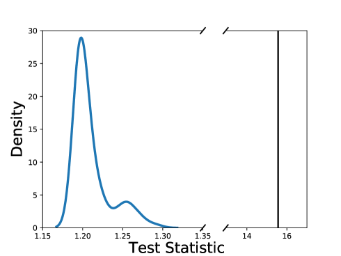
Figure 4: Observed test statistic value (black vertical line) and estimated reference density of the test statistic based on $S=100$ simulations for conflict checking for the biased data example. A broken $x$-axis is used so that the reference density and test statistic can be shown on the same graph.

6 Empirical Examples

In this section we apply our methodology to two real data analyses where cutting feedback affects inference substantially. Code to reproduce the results can be found at https://github.com/Yu-Xuejun/Variational-Cutting-Feedback.

6.1 Human papillomavirus and cervical cancer incidence

We consider an epidemiological example examined by Plummer (2015) and motivated by the study of Maucort-Boulch et al. (2008). The example considers the relationship between human papillomavirus (HPV) prevalence and the incidence of cervical cancer, and the model used corresponds to a two module system of the type described earlier. In this problem there is data $\text{\boldmath$z$}=(z_{1},\dots,z_{13})^{\top}$ for 13 countries from an international survey where $z_{i}$ is the number of people infected with high-risk HPV in a sample of size $n_{i}$. There is also data $\text{\boldmath$w$}=(w_{1},\dots,w_{13})^{\top}$, for which $w_{i}$ is the number of cervical cancer cases diagnosed during $T_{i}$ years of follow-up.

The model is

$$z_{i}\sim\text{Binomial}(n_{i},\gamma_{i}),\quad\gamma_{i}\sim\text{Beta}(1,1),\quad\varphi_{i}=\text{logit}(\gamma_{i}),$$

$$w_{i}\sim\text{Poisson}(\mu_{i}),\quad\mu_{i}=T_{i}\exp(\eta_{1}+\eta_{2}\gamma_{i}),\quad\eta_{1},\eta_{2}\sim\text{N}(0,10^{3}).$$

Here we are particularly interested in $\eta_{2}$, which measures the relationship between HPV prevalence and cancer incidence. However, there is a concern that the Poisson regression model is misspecified, and that this may contaminate inferences for both $\text{\boldmath$\gamma$}=(\gamma_{1},\dots,\gamma_{13})^{\top}$ and $\text{\boldmath$\eta$}=(\eta_{1},\eta_{2})$. We write $\text{\boldmath$\varphi$}=(\varphi_{1},\dots,\varphi_{13})^{\top}$. Although the parameter $\eta_{2}$ is in the misspecified module, having a useful interpretation for it crucially depends on the parameter $\gamma_{i}$ from the correctly specified module having its intended interpretation.

First, consider a prior-data conflict check to help decide whether it is useful to cut. In Figure 5, the blue curve is a kernel density estimate obtained from simulated test statistic values $\widetilde{T}(\text{\boldmath$W$}^{(i)}|\text{\boldmath$z$})$, $i=1,\dots,100$, where $\text{\boldmath$W$}^{(i)}$ are approximate simulations from $p(\text{\boldmath$w$}|\text{\boldmath$z$})$, where the variational approximation for $p(\text{\boldmath$\varphi$}|\text{\boldmath$z$})$ has been used. The black vertical line is the observed test statistic value $\widetilde{T}(\text{\boldmath$w$}|\text{\boldmath$z$})$. Fixed form normal approximations are used for the posterior distribution of $(\text{\boldmath$\varphi$}^{\top},\text{\boldmath$\eta$}^{\top})$ in obtaining the test statistics. Because our variational approximations are normal, the KL divergence terms for computing the test statistics can be evaluated in closed form. The observed test statistic is larger than all simulated values of the test statistic, so that the difference between cut and full posterior distributions is large under the reference distribution. In Appendix B, Figure 11 is similar to Figure 5, except that the data are simulated using the posterior mean values obtained for the real data. Because the data are simulated, there is no misspecification for the Poisson regression in the second module, and Figure 11 demonstrates that the cut and full posterior distributions are not surprisingly different under the reference distribution in this case.

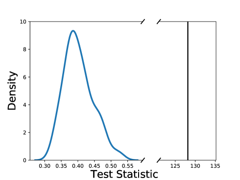
Figure 5: Observed test statistic value (black vertical line) and estimated reference density for the test statistic based on $100$ simulations for conflict check for the HPV example. A broken $x$-axis is used so that the reference density and test statistic can be shown on the same graph.

In Figure 6, the exact full and cut posterior distributions are compared with the variational full and cut posterior distribution approximations. Draws from the full (i.e. uncut) posterior are shown in blue, and draws from the cut posterior in orange. The left panel shows the variational posteriors, while the right panel shows the MCMC (i.e. exact) posteriors. We make two observations. First, the full and cut posterior distributions are quite different, whether computed using MCMC or variational inference methods. This is consistent with the result of the conflict check. Second, the variational approximations are similar to the MCMC estimates of the cut and full posterior distributions, although for the full posterior distribution there is a larger difference between the two approaches.

It takes 14 minutes to run two-stage Monte Carlo sampling for cut posterior computation following the multiple imputation approach of Plummer (2015). Samples of $\varphi$ given $z$ are drawn directly from the exact posterior distribution in a first stage. This can be done because the beta priors on the probabilities $\gamma_{i}$ are conjugate to the binomial likelihood terms. In the second stage, for each first stage sample for $\varphi$, a single chain of length $2,000$ is run with the last value drawn taken as an approximate sample from the conditional posterior for $\eta$ given the fixed value of $\varphi$. The MCMC runs are done using Stan (Carpenter et al., 2017). For variational approximation, the computation time is 68 seconds, using 10,000 stochastic gradient iterations in stage one, and 100,000 stochastic gradient iterations in stage two. Computations were done on an Intel i7-11800H CPU with 8 cores.

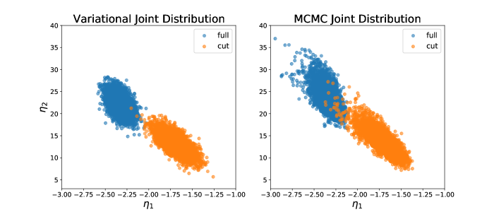
Figure 6: Joint full and cut posteriors of $\eta=(\eta_{1},\eta_{2})$ obtained by fixed form variational approximation and MCMC.

6.2 Agricultural extensification

6.2.1 Two module system

Our last example considers a two module system described in Styring et al. (2017) and Carmona and Nicholls (2020). The data in this example consists of two parts. The first contains measurements relating to agricultural practices and productivity from archaeological sites in Northern Mesopotamia, and the second part contains similar modern data obtained under controlled experimental conditions. An imputation model is used to account for missingness in the archaeological data. One of the parameters in the imputation model, which relates site size to manuring levels, is of primary interest. The interpretation of this parameter can provide evidence for an “extensification hypothesis” of larger land areas being cultivated with lower manure/midden inputs to support growing urban populations. However, the imputation model is rather crude, and it is desirable to cut feedback to ensure that the interpretation of the key parameter is not influenced by this inadequacy.

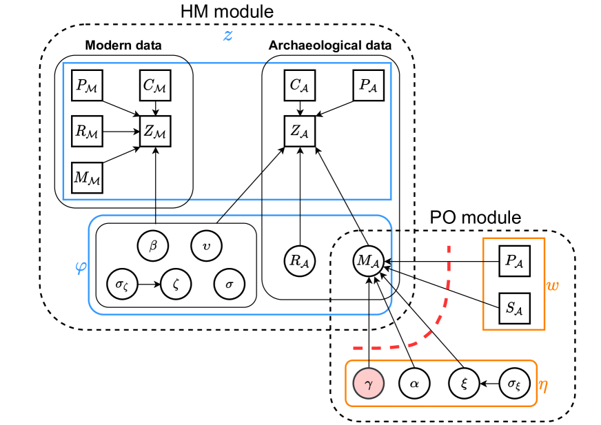
Figure 7: Graphical representation of the two module model for agricultural extensification example. The red dashed line indicates the cut. Squares are known data, while circles are unknown parameters or missing data. The pink circle ($\gamma$) denotes the parameter of interest.

The archaeological dataset contains variables Nitrogen Level ($Z_{\mathcal{A}}$), Crop Category ($C_{\mathcal{A}}$), Site Location ($P_{\mathcal{A}}$) and Site Size ($S_{\mathcal{A}}$). The modern dataset contains the same four variables denoted with subscript $\mathcal{M}$, along with Rainfall ($R_{\mathcal{M}}$) and Manure Level ($M_{\mathcal{M}}$). The latter is an ordinal variable with three possible values $m_{low}<m_{med}<m_{high}$.

A model with two modules is considered here. The first module (labeled the “HM module” here) is a Gaussian linear regression that pools both datasets and has dependent variable Nitrogen Level. There are fixed effects in Rainfall and Manuring Level, a random effect in Site Location and a different error variance depending on Crop Category. In this HM module, Rainfall ($R_{\mathcal{A}}$) and Manure level ($M_{\mathcal{A}}$) in the archaeological data are both missing. The second module is a proportional odds model (labeled the “PO module” here) for imputation of missing values in the archaeological data, with an ordinal response Manure Level. There is a fixed effect in Site Size with coefficient $\gamma$, a random effect in Site Location and a logit link function. If $\gamma<0$, this provides statistical support for the extensification hypothesis. Appendix C details the two modules, along with their likelihood functions and the priors employed. A graphical depiction of the model, similar to Figure 6 in Carmona and Nicholls (2020), is shown in Figure 7.

6.2.2 Cutting feedback

For the full posterior, the PO module plays the role of imputing the missing Manure Level values ($M_{\mathcal{A}}$). However, this model is thought to be misspecified, so we cut feedback from the PO module when imputing $M_{\mathcal{A}}$, so that any misspecification does not affect interpretation of the parameter of primary interest $\gamma$.

The notation of a two module system outlined in Section 2.3 is adopted. This is depicted in Figure 7, where for the HM module the data is denoted as $z$ and unknowns as $\varphi$, while for the PO module the site size and location covariates are denoted as $w$ and parameters as $\eta$. Using this notation, the two module system can be further represented in a simplified form in Figure 8. While this differs slightly from that in Figure 1, the cut posteriors for both cases have the same form. By noting that the data $w$ consists only of covariate data that is observed without error (i.e. it is a deterministic quantity), the joint posterior is given by $p(\text{\boldmath$\eta$},\text{\boldmath$\varphi$}|\text{\boldmath$y$})\propto p(\text{\boldmath$\eta$})p(\text{\boldmath$\varphi$}|\text{\boldmath$\eta$},\text{\boldmath$w$})p(\text{\boldmath$z$}|\text{\boldmath$\varphi$})$. After cutting feedback, the cut posterior is given at (2).

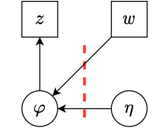
Figure 8: Simplified graphical representation of the two module agriculture model. The red dashed line indicates the cut.

Because $w$ is deterministic, it is not possible to perform the conflict check described in Section 5, because it requires the conditional distribution $p(\text{\boldmath$w$}|\text{\boldmath$z$})$ to give a reference distribution. Therefore, we instead measure conflict for the missing data $M_{\mathcal{A}}$ in the following way. Denote by $M_{\mathcal{A},i}$ the $i$th component of $M_{\mathcal{A}}$, $i=1,\dots,n_{\mathcal{A}}$. Denote by $p_{\text{cut}}(M_{\mathcal{A},i}=m|\text{\boldmath$y$})$ and $p(M_{\mathcal{A},i}=m|\text{\boldmath$y$})$ the probability that $M_{\mathcal{A},i}=m$ under the cut and full posterior distributions, respectively. Write $q_{\text{cut}}(M_{\mathcal{A},i}=m)$ and $q(M_{\mathcal{A},i}=m)$ for their respective variational approximations, which are computed as described below. Figure 9 gives pairwise scatterplots of the probability mass values $\left(q_{\text{cut}}(M_{\mathcal{A},i}=m),q(M_{\mathcal{A},i}=m)\right)$, for all observations in the archaeological data $i=1,\dots,n_{\mathcal{A}}$. For points not close to the diagonal line, it indicates that the imputation for $M_{\mathcal{A}}$ is very different under the cut and full posterior distribution. This is the case here, supporting the decision to cut the posterior in this case.

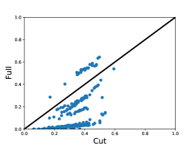
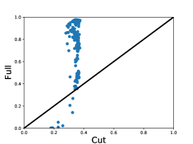
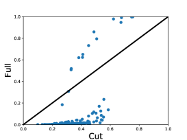
Figure 9: Depiction of the distribution of the (unobserved) manuring level in the archaeological data, estimated using the full and cut variational posteriors. Each panel contains a scatterplot of the probability masses $\left(q_{\text{cut}}(M_{\mathcal{A},i}=m),q(M_{\mathcal{A},i}=m)\right)$, for $i=1,\dots,n_{\mathcal{A}}$. From left to right, the panels correspond to $m=m_{low}$, $m=m_{med}$ and $m=m_{high}$.

6.2.3 Variational inference

A two-stage variational optimization is performed to get a Gaussian approximation of the posterior of the continuous parameters for the cut model. Parameters in the HM module are updated by the first-stage optimization whereas those in the PO module are updated by the second-stage optimization with $M_{\mathcal{A}}$ fixed to be the variational posterior samples obtained by the first stage. The difficulty in this example is that, in the HM module, the three-level discrete missing value $M_{\mathcal{A}}$ cannot be approximated by a Gaussian distribution. In this case, we use a method recently developed by Loaiza-Maya et al. (2021) which treats $M_{\mathcal{A}}$ as a latent variable and updates it by Monte Carlo generation, while updating the variational parameters by stochastic optimization as we now discuss.

In the HM module the unknowns are $\text{\boldmath$\varphi$}=(\text{\boldmath$\rho$}^{\top},M_{\mathcal{A}}^{\top})^{\top}$, where $\rho$ denotes all the unknowns other than $M_{\mathcal{A}}$. The posterior density $p(\text{\boldmath$\varphi$}|\text{\boldmath$z$})=p(\text{\boldmath$\rho$},M_{\mathcal{A}}|\text{\boldmath$z$})\propto p(\text{\boldmath$z$}|\text{\boldmath$\rho$},M_{\mathcal{A}})p(M_{\mathcal{A}}|\text{\boldmath$\rho$})p(\text{\boldmath$\rho$})\equiv g(\text{\boldmath$\rho$},M_{\mathcal{A}})$ can be approximated by the variational density

$$q_{\text{\boldmath$\lambda$}}(\text{\boldmath$\rho$},M_{\mathcal{A}})=p(M_{\mathcal{A}}|\text{\boldmath$\rho$},\text{\boldmath$z$})q^{0}_{\text{\boldmath$\lambda$}}(\text{\boldmath$\rho$})\,.$$ (21)

A Gaussian variational approximation $q^{0}_{\text{\boldmath$\lambda$}}(\text{\boldmath$\rho$})=\phi(\text{\boldmath$\rho$};\text{\boldmath$\mu$},\text{\boldmath$C$}\text{\boldmath$C$}^{\top})$ is adopted for $\rho$, while the exact conditional posterior is used for $M_{\mathcal{A}}$. Loaiza-Maya et al. (2021) show that (21) is an accurate variational approximation, and that Algorithm 2 is a fast stochastic gradient ascent algorithm to minimize the variational lower bound. At step (2) of this algorithm, $M_{\mathcal{A}}$ is generated from its conditional posterior which is available analytically here. In step (3), it is possible to use automatic differentiation tools for computing the gradient estimate with the discrete samples. In step (4), the step sizes are obtained adaptively using the ADADELTA method (Zeiler, 2012). We keep the last 10000 updates of $\text{\boldmath$\varphi$}=(\text{\boldmath$\rho$},M_{\mathcal{A}})$ as a sample from the variational posterior, and randomly draw from it in each update in the second-stage optimization for the PO module, so as to account for posterior uncertainty in the HM module.

Algorithm 2 Variational Inference with Latent Variables $M_{\mathcal{A}}$

  Initialize $\text{\boldmath$\lambda$}=(\text{\boldmath$\mu$},\text{\boldmath$C$})$, $M_{\mathcal{A}}$, run-length $K$

  for $k=1:K$ do

     (1) Generate $\text{\boldmath$\epsilon$}\sim\text{N}(\bm{0},I)$ and set $\text{\boldmath$\rho$}=\text{\boldmath$C$}\text{\boldmath$\epsilon$}+\text{\boldmath$\mu$}$

     (2) Generate $M_{\mathcal{A}}\sim p(M_{\mathcal{A}}|\text{\boldmath$\rho$},\text{\boldmath$z$})$ exactly

     (3) Compute an unbiased estimate of the lower bound gradient,

$$\widehat{\nabla_{\lambda}{\cal L}(\lambda)}=\frac{d\text{\boldmath$\rho$}}{d\text{\boldmath$\lambda$}}^{\top}\left\{\nabla_{\text{\boldmath$\rho$}}\log g(\text{\boldmath$\rho$},M_{\mathcal{A}})-\nabla_{\text{\boldmath$\rho$}}\log q_{\text{\boldmath$\lambda$}}^{0}(\text{\boldmath$\rho$})\right\}$$

     (4) Update

$$\text{\boldmath$\lambda$}=\text{\boldmath$\lambda$}+\text{\boldmath$s$}_{k}\circ\widehat{\nabla_{\lambda}{\cal L}(\lambda)},$$

where $\text{\boldmath$s$}_{k}$ is a vector of step sizes at iteration $k$ and $\circ$ denotes elementwise product for two vectors.

  end for

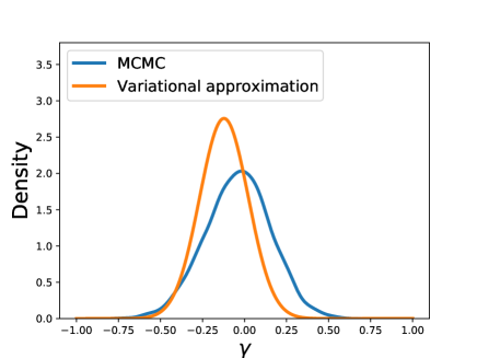
(a) Cut posterior of $\gamma$.

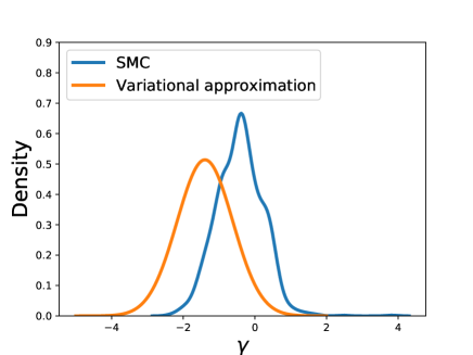
(b) Full posterior of $\gamma$.

Figure 10: Posterior of $\gamma$ obtained by cut model (left) and full model (right).

Figure 10 shows the marginal full and cut posterior densities for $\gamma$ obtained by variational approximation and exact-in-principle Monte Carlo methods. For comparison with the variational methods, MCMC was used to approximate the cut posterior distribution, and a sequential Monte Carlo (SMC) sampler (Del Moral et al., 2006) for the full posterior distribution. The full posterior is complex, and we found it necessary to use the SMC sampler instead of MCMC to evaluate it reliably. The posterior densities obtained using variational approximation and MCMC are shown by orange and blue lines, respectively. We make two observations. First, the variational posterior distributions for $\gamma$ are similar to those obtained by MCMC for the cut distribution, with a larger difference between the variational and SMC method for the full posterior distribution. Second, the inferences are very different for the cut and full posterior distributions. The inferences we obtain for the cut model are similar to those in Carmona and Nicholls (2020), although we have used different priors in our analysis. In the semi-modular inference approach of Carmona and Nicholls (2020) they consider partially cutting feedback, with the amount of feedback chosen according to predictive criteria. This results in a posterior probability of $\gamma<0$ (supporting the extensification hypothesis) somewhere in between those for the cut and full posterior distributions.

The computation time for cut posterior approximation using the two-stage variational approach and MCMC are as follows. For a multiple imputation MCMC approach (Plummer, 2015) samples are generated for $\varphi$ from $p(\text{\boldmath$\varphi$}|\text{\boldmath$z$})$ in a first stage. This takes 21 hours for MCMC with 100,000 iterations and 2 chains. We retain $1,000$ samples from the first stage. At a second stage, generating an approximate conditional full posterior sample of $\eta$ for each of the first stage $\varphi$ samples takes 33 minutes using a single chain of length $10,000$ and retaining the last value. In the two-stage variational approach, the first stage takes 93 minutes in stage one and 3 minutes in stage two for 100,000 stochastic gradient ascent iterations in each case. Computations were done on an Intel i7-11800H CPU with 8 cores.

The full and cut posterior densities in this example are complex. In examples like this one, the reader might wonder what happens if the approximating family is poorly chosen. In this case, if the conventional KL variational objective is used, then underestimation of uncertainty is a common result, although variational point estimates can still perform well. Many authors have considered using alternative divergence measures in variational inference, which may result in approximations which are mass-covering. However, for these alternative approaches stable optimization in high dimensions can be challenging.

7 Discussion

Variational methods have strong potential in modularized inference, including the case in which cutting feedback between modules is required. This paper develops cut procedures using variational inference methods which have reduced computational demands compared to existing MCMC implementations. We consider both cut procedures defined through modifications of variational message passing, as well as explicit formulations of cutting feedback where the cut posterior can be defined as the solution of a constrained optimization problem. In the explicit formulation, it is convenient to use fixed form variational approximations based on a sequential decomposition, which also leads to practical variational implementations of computationally burdensome checks for conflicting information that are useful in making the decision of whether or not to cut.

In the message passing formulation of cutting feedback there are alternative possible implementations that have not been explored here, and we leave this to future work. Our work has mostly used simple Gaussian approximations to facilitate the conflict checks discussed in Section 4, where the ability to explicitly compute KL divergences is an advantage. Further interesting work could be done on using more flexible variational families, similar to the last example of Section 5 where we considered combining MCMC and variational inference methods using the approach of Loaiza-Maya et al. (2021). The recent work in Carmona and Nicholls (2022) using normalizing flows is another promising direction. It is interesting to ask whether variational message passing or stochastic gradient cut methods are preferred when both can be implemented. In the two module case, there can be strong dependence between $\varphi$ and $\eta$, and this makes a factorized approximation in variational message passing unattractive. The generality and ease of implementation of stochastic gradient optimization using automatic differentiation tools make stochastic gradient cut approximations the preferred approach in many situations. However, we do think the variational message passing approach may have uses in complex situations beyond the two module case.

Appendix A: Variational message passing for biased data example

In the biased data example, data likelihoods and priors can be summarized as follows

$$\text{\boldmath$z$}=(z_{1},\dots,z_{n_{1}})|\varphi\sim N(\varphi,1)\quad i.i.d,\quad\varphi\sim N(0,\delta_{1}^{-1}),$$

$$\text{\boldmath$w$}=(w_{1},\dots,w_{n_{2}})|\varphi,\eta\sim N(\varphi+\eta,1)\quad i.i.d,\quad\eta\sim N(0,\delta_{2}^{-1}),$$

where $\delta_{1}$ and $\delta_{2}$ are known.

The variational joint posterior at (8) has the form

$$q(\varphi,\eta)=q_{\varphi}(\varphi)q_{\eta}(\eta).$$

The coordinate ascent updates for $q_{\varphi}(\varphi)$ and $q_{\eta}(\eta)$ for approximating the full posterior can be written as

$$q_{\varphi}(\varphi) \propto m_{p(\varphi)\rightarrow\varphi}(\varphi)\times m_{p(\text{\boldmath$z$}|\varphi)\rightarrow\varphi}(\varphi)\times m_{p(\text{\boldmath$w$}|\varphi,\eta)\rightarrow\varphi}(\varphi),$$

$$q_{\eta}(\eta) \propto m_{p(\eta)\rightarrow\eta}(\eta)\times m_{p(\text{\boldmath$w$}|\varphi,\eta)\rightarrow\eta}(\eta).$$

where

$$m_{p(\varphi)\rightarrow\varphi}(\varphi) =\exp\left(E_{q_{\eta}}(\log p(\varphi))\right)=p(\varphi)=\sqrt{\frac{\delta_{1}}{2\pi}}\exp(-\frac{1}{2}\delta_{1}\varphi^{2}),$$

$$m_{p(\eta)\rightarrow\eta}(\eta) =\exp\left(E_{q_{\varphi}}(\log p(\eta))\right)=p(\eta)=\sqrt{\frac{\delta_{2}}{2\pi}}\exp(-\frac{1}{2}\delta_{2}\eta^{2}),$$

$$m_{p(\text{\boldmath$z$}|\varphi)\rightarrow\varphi}(\varphi) =\exp\left(E_{q_{\eta}}(\log p(\text{\boldmath$z$}|\varphi))\right)=p(\text{\boldmath$z$}|\varphi)=\frac{n_{1}}{\sqrt{2\pi}}\exp(-\frac{1}{2}\sum_{i=1}^{n_{1}}(z_{i}-\varphi)^{2}),$$

$$m_{p(\text{\boldmath$w$}|\varphi,\eta)\rightarrow\varphi}(\varphi) =\exp\left(E_{q_{\eta}}(\log p(\text{\boldmath$w$}|\varphi,\eta))\right)$$

$$=\exp(-\frac{n_{2}}{2}\log(2\pi)-\frac{1}{2}\sum_{i=1}^{n_{2}}E_{q_{\eta}}[(w_{i}-\varphi-\eta)^{2}])$$

$$=\exp(-\frac{n_{2}}{2}\log(2\pi)-\frac{1}{2}\sum_{i=1}^{n_{2}}[Var_{q_{\eta}}(\eta)+(w_{i}-\varphi-E_{q_{\eta}}(\eta))^{2}]),$$

$$m_{p(\text{\boldmath$w$}|\varphi,\eta)\rightarrow\eta}(\eta) =\exp\left(E_{q_{\varphi}}(\log p(\text{\boldmath$w$}|\varphi,\eta))\right)$$

$$=\exp(-\frac{n_{2}}{2}\log(2\pi)-\frac{1}{2}\sum_{i=1}^{n_{2}}E_{q_{\varphi}}[(w_{i}-\varphi-\eta)^{2}])$$

$$=\exp(-\frac{n_{2}}{2}\log(2\pi)-\frac{1}{2}\sum_{i=1}^{n_{2}}[Var_{q_{\varphi}}(\varphi)+(w_{i}-E_{q_{\varphi}}(\varphi)-\eta)^{2}]).$$

Thus,

$$q^{*}(\varphi) \propto m_{p(\varphi)\rightarrow\varphi}(\varphi)\times m_{p(\text{\boldmath$z$}|\varphi)\rightarrow\varphi}(\varphi)\times m_{p(\text{\boldmath$w$}|\varphi,\eta)\rightarrow\varphi}(\varphi)$$

$$\propto\exp(-\frac{\delta_{1}}{2}\varphi^{2})\exp(-\frac{1}{2}\sum_{i=1}^{n_{1}}(z_{i}-\varphi)^{2})\exp(-\frac{1}{2}\sum_{i=1}^{n_{2}}(w_{i}-\varphi-E_{q_{\eta}}(\eta))^{2})$$

$$\propto\exp(-\frac{1}{2}[(\delta_{1}+n_{1}+n_{2})\varphi^{2}-2(\sum_{i=1}^{n_{1}}z_{i}+\sum_{i=1}^{n_{2}}(w_{i}-E_{q_{\eta}}(\eta))\varphi]),$$

$$q^{*}(\eta) \propto m_{p(\eta)\rightarrow\eta}(\eta)\times m_{p(\text{\boldmath$w$}|\varphi,\eta)\rightarrow\eta}(\eta)$$

$$\propto\exp(-\frac{\delta_{2}}{2}\eta^{2})\exp(-\frac{1}{2}\sum_{i=1}^{n_{2}}(w_{i}-E_{q_{\varphi}}(\varphi)-\eta)^{2})$$

$$\propto\exp(-\frac{1}{2}[(\delta_{2}+n_{2})\eta^{2}-2(\sum_{i=1}^{n_{2}}(w_{i}-E_{q_{\varphi}}(\varphi)))\eta]).$$

The variational posterior densities of $\varphi$ and $\eta$ are both normal distributions. To update them, we only need to update means and variances by

$$E_{q_{\varphi}}(\varphi)=\frac{n_{1}\bar{\text{\boldmath$z$}}+n_{2}\bar{\text{\boldmath$w$}}-n_{2}E_{q_{\eta}}(\eta)}{\delta_{1}+n_{1}+n_{2}},\quad\quad Var_{q_{\varphi}}(\varphi)=\frac{1}{\delta_{1}+n_{1}+n_{2}},$$

$$E_{q_{\eta}}(\eta)=\frac{n_{2}\bar{\text{\boldmath$w$}}-n_{2}E_{q_{\varphi}}(\varphi)}{\delta_{2}+n_{2}},\quad\quad Var_{q_{\eta}}(\eta)=\frac{1}{\delta_{2}+n_{2}}.$$

The cut marginal posterior density for $\varphi$ is just $p(\varphi|z)$ by the discussion in Section 3.3. Hence after some simple algebra

$$q_{\text{cut},\varphi}(\varphi)=p(\varphi|z)=\phi\left(\varphi;(n_{1}+\delta_{1})^{-1}n_{1}\bar{z},(n_{1}+\delta_{1})^{-1}\right).$$

To get $q_{\text{cut},\eta}(\eta)$, we plug the posterior mean of $\varphi$ from the cut posterior density into $q^{*}(\eta)$ to obtain

$$q_{\text{cut},\eta}(\eta)=\phi\left(\eta;(n_{2}+\delta_{2})^{-1}n_{2}(\bar{w}-(n_{1}+\delta_{1})^{-1}n_{1}\bar{z}),(n_{2}+\delta_{2})^{-1}\right).$$

The exact joint cut posterior density is $p(\varphi|z)p(\eta|\varphi,w)$, where $p(\varphi|z)$ is given above, and

$$p(\eta|\varphi,w) \propto p(\eta)p(w|\varphi,\eta),$$

which simplifies after some algebra to

$$p(\eta|\varphi,w)=\phi\left(\eta;(\delta_{2}+n_{2})^{-1}n_{w}(\bar{w}-\varphi),(\delta+n_{2})^{-1}\right).$$

We can see that $q_{\text{cut},\eta}(\eta)=p(\eta|\varphi=\mu_{\varphi},w)$, where $\mu_{\varphi}=n_{1}\bar{z}/(n_{1}+\delta_{1})$. So the cut marginal variational posterior density for $\eta$ is obtained by plugging in a point estimate of $\varphi$ to the posterior full conditional for $\eta$.

Finally, the exact Bayes posterior is

$$p(\varphi|z,w)p(\eta|\varphi,w),$$

with $p(\eta|\varphi,w)$ given above,and

$$p(\varphi|z,w)=\phi\left(\left(n_{1}+\delta_{1}+\frac{n_{2}\delta_{2}}{\delta_{2}+n_{2}}\right)^{-1}\left(n_{1}\bar{z}+\frac{n_{2}\delta_{2}}{\delta_{2}+n_{2}}\bar{w}\right),\left(n_{1}+\delta_{1}+\frac{n_{2}\delta_{2}}{\delta_{2}+n_{2}}\right)^{-1}\right).$$

It can be seen from this expression that if $n_{2}$ and $\delta_{2}$ are large, then the posterior mean for $\varphi$ will be dominated by the sample mean obtained from the biased data.

Appendix B: Conflict checking for simulated data, HPV example

For the posterior mean parameter values obtained via MCMC for the HPV example of Section 6.1, we simulated a replicate dataset. Since the data are simulated, there is no misspecification of the likelihood in the second module. We then repeated the conflict check shown in Figure 5, for the simulated data. The result is shown in Figure 11. As might be expected, the difference between the full and cut variational posterior distribution is not large compared to the reference distribution in this setting of correct model specification.

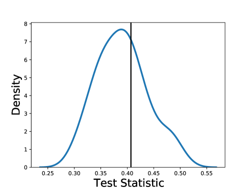
Figure 11: Observed test statistic value (black vertical line) and estimated reference density for the test statistic based on $100$ simulations for conflict check for the simulated HPV example.

Appendix C: Agricultural extensification model

In this appendix we detail the model employed in the agricultural extensification example. It consists of two modules: a regression model (HM module) used to impute the missing Manure Level observations in the archaeological dataset ($M_{\mathcal{A}}$), and a proportional odds model (PO module) used to specify the parameter $\gamma$ that is employed to assess the hypothesis of extensification. The likelihoods and priors of the HM and PO modules are specified below, from which both the cut and full variational posteriors can be obtained.

C.1: HM module

The HM module is a linear Gaussian regression that pools both the archaeological data $\mathcal{A}$ and modern data $\mathcal{M}$. The response is Nitrogen Level ($Z_{d,i}$), and there are fixed effects in Rainfall ($R_{d,i}$) and Manure Level ($M_{d,i}$), as well as a random effect in Site Location ($P_{d,i}$), where $d={\mathcal{A}},\mathcal{M}$ indexes the dataset and $i=1,\ldots,n_{d}$ the observation. The Manure Level is a categorical variable where $M_{d,i}\in\{m_{low},m_{med},m_{high}\}$ with $m_{low}<m_{med}<m_{high}$. Dummy variables $D_{d,i}^{med}=\mathbbm{1}(M_{d,i}=m_{med})$ and $D_{d,i}^{high}=\mathbbm{1}(M_{d,i}=m_{high})$ are introduced for medium $m_{med}$ and high $m_{high}$ manuring levels (with low manuring level $m_{low}$ acting as the baseline category). There are $q_{2}=24$ site locations, so that if $l(d,i)$ is the location of site $P_{d,i}$ then the regression is

$$Z_{d,i}=(1,R_{d,i},D_{d,i}^{med},D_{d,i}^{high})^{\top}\text{\boldmath$\beta$}+\zeta_{l(d,i)}+\epsilon_{d,i}\,,$$ (22)

where $\bm{\beta}=(\beta_{1},\dots,\beta_{4})^{\top}$ are fixed effects coefficients, and $\zeta_{l}\sim\text{N}(0,\sigma^{2}_{\zeta})$ are the $l=1,\ldots,q_{2}$ location random effect values. The errors are heteroscedastic, with $\epsilon_{d,i}\sim\text{N}(0,\sigma^{2})$ if the $(d,i)$th observation has Crop Category $C_{d,i}$ given by barley, and $\epsilon_{d,i}\sim\text{N}(0,\upsilon\sigma^{2})$ if wheat.

Conditional on the $n_{\mathcal{A}}$ observations on the Manuring Level $M_{\mathcal{A}}$ and Rainfall $R_{\mathcal{A}}$, as well as the random effect values $\bm{\zeta}=(\zeta_{1},\ldots,\zeta_{q_{2}})^{\top}$, the likelihood of the HM module is simply given by the product of $n_{\mathcal{A}}+n_{\mathcal{M}}$ Gaussian densities specified at (22).

Given a large number $g=1000$, the following priors are used:

$$M_{\mathcal{A},i}\sim{\cal U}\left\{1,3\right\},\quad\text{\boldmath$\beta$}\sim\text{N}(\bm{0},gI_{4}),\quad\sigma^{2}\sim\text{U}(0.1,5),$$

$$\sigma_{\zeta}^{2}\sim\text{U}(0.1,5),\quad\widetilde{\upsilon}=\log\upsilon\sim\text{N}(0,g).$$

For $\log R_{\mathcal{A}}$, we use normal priors for the components, where the component-specific means and variances match those of the uniform priors used in Styring et al. (2017) (Figure 18 of the supplementary information). Define $\widetilde{\sigma}=\log\frac{\sigma^{2}-0.1}{5-\sigma^{2}}$, $\widetilde{\sigma_{\zeta}}=\log\frac{\sigma_{\zeta}^{2}-0.1}{5-\sigma_{\zeta}^{2}}$ and $\widetilde{\upsilon}=\log\upsilon$, so that $\widetilde{\sigma}$, $\widetilde{\sigma_{\zeta}}$ and $\widetilde{\upsilon}$ are unconstrained and suitably approximated by a Gaussian. Then parameters and unknown quantities in the HM module can be summarized as $\text{\boldmath$\varphi$}=(\text{\boldmath$\rho$}^{\top},M_{\mathcal{A}}^{\top})^{\top}$, where $\text{\boldmath$\rho$}=(\log(R_{\mathcal{A}})^{\top},\text{\boldmath$\beta$}^{\top},\sigma,\text{\boldmath$\zeta$}^{\top},\sigma_{\zeta},\upsilon)^{\top}$.

C.2: PO Module

The PO module is a proportional odds model applied only to the archaeological data with an ordinal response Manure Level ($M_{\mathcal{A},i}$), a fixed effect for Site Size ($S_{\mathcal{A},i}$), random effect for Site Location ($P_{\mathcal{A},i}$), and a logit link function. Let $p_{m}(P,S)={\rm Pr}(M\leq m|P,S)$ be the cumulative distribution function of Manure Level $M$ at level $m$ from an observation with Site Size $S$ and Location $P$. Then for the observations $i=1,\dots,n_{\mathcal{A}}$, the proportional odds model has the form

$$\log\left(\frac{p_{m}(P_{\mathcal{A},i},S_{\mathcal{A},i})}{1-p_{m}(P_{\mathcal{A},i},S_{\mathcal{A},i})}\right)=\alpha_{m}-\gamma S_{\mathcal{A},i}-\xi_{l(\mathcal{A},i)}\,.$$

There are only five locations in the archaeological dataset, so that the site location random effect values are $\text{\boldmath$\xi$}=(\xi_{1},\ldots,\xi_{5})^{\top}\sim\text{N}(\bm{0},\sigma_{\xi}^{2}I_{5})$. The coefficient $\alpha_{m}\in\left\{\alpha_{low},\alpha_{med}\right\}$ varies according to the manure level value $m$, and $\gamma$ measures the effect of site size.

Define $\mbox{p}_{m,i}\equiv\mbox{Pr}(M_{\mathcal{A},i}\leq m|P_{\mathcal{A},i},S_{\mathcal{A},i})$, and the dummy variable $D_{\mathcal{A},i}^{low}=1-D_{\mathcal{A},i}^{med}-D_{\mathcal{A},i}^{high}$. Then

$$p(M_{\mathcal{A}}|\text{\boldmath$\alpha$},\gamma,\text{\boldmath$\xi$},\sigma_{\xi})=\prod_{i=1}^{n_{\mathcal{A}}}\left(\mbox{p}_{low,i}\right)^{D_{\mathcal{A},i}^{low}}\left(\mbox{p}_{med,i}-\mbox{p}_{low,i}\right)^{D_{\mathcal{A},i}^{med}}\left(1-\mbox{p}_{med,i}\right)^{D_{\mathcal{A},i}^{high}}.$$

Define $\tilde{\alpha}_{med}=\log(\alpha_{med}-\alpha_{low})$ and $\tilde{\sigma_{\xi}}=\log\frac{\sigma_{\xi}}{3.5-\sigma_{\xi}}$, so that $\tilde{\alpha}_{med}$ and $\tilde{\sigma_{\xi}}$ are unconstrained and suitably approximated as Gaussian. Let $\text{\boldmath$\alpha$}=(\alpha_{low},\tilde{\alpha}_{med})^{\top}$, then the parameters in PO module are $\text{\boldmath$\eta$}=(\gamma,\text{\boldmath$\alpha$}^{\top},\text{\boldmath$\xi$}^{\top},\sigma_{\xi})^{\top}$. The following priors are used:

$$\gamma\sim\text{N}(0,4),\quad\alpha_{low}\sim\text{N}(0,1.5),\quad\tilde{\alpha}_{med}\sim\text{N}(-5,7),\quad\sigma_{\xi}\sim\text{U}(0,3.5)\,.$$

References

- Alquier et al. (2016) Alquier, P., J. Ridgway, and N. Chopin (2016). On the properties of variational approximations of Gibbs posteriors. Journal of Machine Learning Research 17(236), 1–41.
- Bennett and Wakefield (2001) Bennett, J. and J. Wakefield (2001). Errors-in-variables in joint population pharmacokinetic/pharmacodynamic modeling. Biometrics 57(3), 803–812.
- Bissiri et al. (2016) Bissiri, P. G., C. C. Holmes, and S. G. Walker (2016). A general framework for updating belief distributions. Journal of the Royal Statistical Society: Series B (Statistical Methodology) 78(5), 1103–1130.
- Blangiardo et al. (2011) Blangiardo, M., A. Hansell, and S. Richardson (2011). A Bayesian model of time activity data to investigate health effect of air pollution in time series studies. Atmospheric Environment 45(2), 379–386.
- Blei et al. (2017) Blei, D. M., A. Kucukelbir, and J. D. McAuliffe (2017). Variational inference: A review for statisticians. Journal of the American Statistical Association 112(518), 859–877.
- Carmona and Nicholls (2020) Carmona, C. and G. Nicholls (2020). Semi-modular inference: Enhanced learning in multi-modular models by tempering the influence of components. In S. Chiappa and R. Calandra (Eds.), Proceedings of the Twenty Third International Conference on Artificial Intelligence and Statistics, Volume 108 of Proceedings of Machine Learning Research, pp. 4226–4235. PMLR.
- Carmona and Nicholls (2022) Carmona, C. and G. Nicholls (2022). Scalable semi-modular inference with variational meta-posteriors. arXiv:2204.00296.
- Carpenter et al. (2017) Carpenter, B., A. Gelman, M. D. Hoffman, D. Lee, B. Goodrich, M. Betancourt, M. Brubaker, J. Guo, P. Li, and A. Riddell (2017, January). Stan: A Probabilistic Programming Language. Journal of Statistical Software 76(1), 1–32.
- Del Moral et al. (2006) Del Moral, P., A. Doucet, and A. Jasra (2006). Sequential Monte Carlo samplers. Journal of the Royal Statistical Society: Series B 68(3), 411–436.
- Evans (2015) Evans, M. (2015). Measuring Statistical Evidence Using Relative Belief. Taylor & Francis.
- Frazier et al. (2021) Frazier, D. T., R. Loaiza-Maya, G. M. Martin, and B. Koo (2021). Loss-based variational Bayes prediction. arXiv:2104.14054.
- Frazier and Nott (2022) Frazier, D. T. and D. J. Nott (2022). Cutting feedback and modularized analyses in generalized Bayesian inference. arXiv:2202.09968.
- Gelman et al. (1996) Gelman, A., X.-L. Meng, and H. Stern (1996). Posterior predictive assessment of model fitness via realized discrepancies. Statistica Sinica 6, 733–807.
- Han et al. (2016) Han, S., X. Liao, D. Dunson, and L. Carin (2016, 09–11 May). Variational Gaussian copula inference. In A. Gretton and C. C. Robert (Eds.), Proceedings of the 19th International Conference on Artificial Intelligence and Statistics, Volume 51 of Proceedings of Machine Learning Research, Cadiz, Spain, pp. 829–838. PMLR.
- Jacob et al. (2017) Jacob, P. E., L. M. Murray, C. C. Holmes, and C. P. Robert (2017). Better together? Statistical learning in models made of modules. arXiv:1708.08719.
- Jacob et al. (2020) Jacob, P. E., J. O’Leary, and Y. F. Atchadé (2020). Unbiased Markov chain Monte Carlo methods with couplings (with discussion). Journal of the Royal Statistical Society: Series B (Statistical Methodology) 82(3), 543–600.
- Kennedy and O’Hagan (2001) Kennedy, M. C. and A. O’Hagan (2001). Bayesian calibration of computer models. Journal of the Royal Statistical Society: Series B (Statistical Methodology) 63(3), 425–464.
- Knoblauch et al. (2019) Knoblauch, J., J. Jewson, and T. Damoulas (2019). Generalized variational inference: Three arguments for deriving new posteriors. arXiv:1904.02063.
- Knowles and Minka (2011) Knowles, D. A. and T. Minka (2011). Non-conjugate variational message passing for multinomial and binary regression. In J. Shawe-Taylor, R. S. Zemel, P. L. Bartlett, F. Pereira, and K. Q. Weinberger (Eds.), Advances in Neural Information Processing Systems 24, pp. 1701–1709. Curran Associates, Inc.
- Kucukelbir et al. (2017) Kucukelbir, A., D. Tran, R. Ranganath, A. Gelman, and D. M. Blei (2017). Automatic differentiation variational inference. Journal of Machine Learning Research 18(14), 1–45.
- Lin et al. (2019) Lin, W., M. E. Khan, and M. Schmidt (2019). Fast and simple natural-gradient variational inference with mixture of exponential-family approximations. In K. Chaudhuri and R. Salakhutdinov (Eds.), Proceedings of the 36th International Conference on Machine Learning, Volume 97 of Proceedings of Machine Learning Research, pp. 3992–4002. PMLR.
- Little (1992) Little, R. J. A. (1992). Regression with missing X’s: A review. Journal of the American Statistical Association 87(420), 1227–1237.
- Liu et al. (2009) Liu, F., M. J. Bayarri, and J. O. Berger (2009). Modularization in Bayesian analysis, with emphasis on analysis of computer models. Bayesian Analysis 4(1), 119–150.
- Liu and Goudie (2020) Liu, Y. and R. J. B. Goudie (2020). Stochastic approximation cut algorithm for inference in modularized Bayesian models. arXiv:2006.01584.
- Liu and Goudie (2021) Liu, Y. and R. J. B. Goudie (2021). Generalized geographically weighted regression model within a modularized bayesian framework. arXiv:2106.00996.
- Loaiza-Maya et al. (2021) Loaiza-Maya, R., M. S. Smith, D. J. Nott, and P. J. Danaher (2021). Fast and accurate variational inference for models with many latent variables. Journal of Econometrics (in press).
- Lunn et al. (2009) Lunn, D., N. Best, D. Spiegelhalter, G. Graham, and B. Neuenschwander (2009). Combining MCMC with ‘sequential’ PKPD modelling. Journal of Pharmacokinetics and Pharmacodynamics 36, 19–38.
- Maucort-Boulch et al. (2008) Maucort-Boulch, D., S. Franceschi, and M. Plummer (2008). International correlation between human papillomavirus prevalence and cervical cancer incidence. Cancer Epidemiology and Prevention Biomarkers 17(3), 717–720.
- McCandless et al. (2010) McCandless, L., I. Douglas, S. Evans, and L. Smeeth (2010). Cutting feedback in Bayesian regression adjustment for the propensity score. The international journal of biostatistics 6, Article 16.
- McCandless et al. (2012) McCandless, L. C., S. Richardson, and N. Best (2012). Adjustment for missing confounders using external validation data and propensity scores. Journal of the American Statistical Association 107(497), 40–51.
- Minka (2005) Minka, T. (2005). Divergence measures and message passing. Technical Report MSR-TR-2005-173, Microsoft Research.
- Moss and Rousseau (2022) Moss, D. and J. Rousseau (2022). Efficient Bayesian estimation and use of cut posterior in semiparametric hidden markov models. arXiv:2203.06081.
- Murphy and Topel (2002) Murphy, K. and R. Topel (2002). Estimation and inference in two-step econometric models. Journal of Business and Economic Statistics 20(1), 88–97.
- Nicholls et al. (2022) Nicholls, G. K., J. E. Lee, C.-H. Wu, and C. U. Carmona (2022). Valid belief updates for prequentially additive loss functions arising in semi-modular inference. arXiv preprint arXiv:2201.09706.
- Nicholson et al. (2021) Nicholson, G., M. Blangiardo, M. Briers, P. J. Diggle, T. E. Fjelde, H. Ge, R. J. B. Goudie, R. Jersakova, R. E. King, B. C. L. Lehmann, A.-M. Mallon, T. Padellini, Y. W. Teh, C. Holmes, and S. Richardson (2021). Interoperability of statistical models in pandemic preparedness: principles and reality. arXiv:2109.13730.
- Nott et al. (2020) Nott, D. J., X. Wang, M. Evans, and B.-G. Englert (2020). Checking for prior-data conflict using prior-to-posterior divergences. Statistical Science 35(2), 234–253.
- Ogle et al. (2013) Ogle, K., J. Barber, and K. Sartor (2013). Feedback and modularization in a Bayesian meta–analysis of tree traits affecting forest dynamics. Bayesian Analysis 8(1), 133 – 168.
- Ormerod and Wand (2010) Ormerod, J. and M. Wand (2010). Explaining variational approximations. The American Statistician 64, 140–153.
- Papamakarios et al. (2021) Papamakarios, G., E. Nalisnick, D. J. Rezende, S. Mohamed, and B. Lakshminarayanan (2021). Normalizing flows for probabilistic modeling and inference. Journal of Machine Learning Research 22(57), 1–64.
- Petrin and Train (2010) Petrin, A. and K. Train (2010). A control function approach to endogeneity in consumer choice models. Journal of Marketing Research 47(1), 3–13.
- Plummer (2015) Plummer, M. (2015). Cuts in Bayesian graphical models. Statistics and Computing 25, 37–43.
- Pompe and Jacob (2021) Pompe, E. and P. E. Jacob (2021). Asymptotics of cut distributions and robust modular inference using posterior bootstrap. arXiv:2110.11149.
- Presanis et al. (2013) Presanis, A. M., D. Ohlssen, D. J. Spiegelhalter, and D. D. Angelis (2013). Conflict diagnostics in directed acyclic graphs, with applications in Bayesian evidence synthesis. Statistical Science 28, 376–397.
- Salimans et al. (2013) Salimans, T., D. A. Knowles, et al. (2013). Fixed-form variational posterior approximation through stochastic linear regression. Bayesian Analysis 8(4), 837–882.
- Smith et al. (2020) Smith, M. S., R. Loaiza-Maya, and D. J. Nott (2020). High-dimensional copula variational approximation through transformation. Journal of Computational and Graphical Statistics 29(4), 729–743.
- Styring et al. (2017) Styring, A., M. Charles, F. Fantone, M. Hald, A. McMahon, R. Meadow, G. Nicholls, A. Patel, M. Pitre, A. Smith, A. Sołtysiak, G. Stein, J. Weber, H. Weiss, and A. Bogaard (2017). Isotope evidence for agricultural extensification reveals how the world’s first cities were fed. Nature Plants 3, 17076.
- Titsias and Lázaro-Gredilla (2014) Titsias, M. and M. Lázaro-Gredilla (2014). Doubly stochastic variational Bayes for non-conjugate inference. In E. P. Xing and T. Jebara (Eds.), Proceedings of the 31st International Conference on Machine Learning, Volume 32 of Proceedings of Machine Learning Research, Bejing, China, pp. 1971–1979. PMLR.
- Wand (2017) Wand, M. P. (2017). Fast approximate inference for arbitrarily large semiparametric regression models via message passing. Journal of the American Statistical Association 112(517), 137–168.
- Wang and Blei (2019) Wang, Y. and D. M. Blei (2019). Variational Bayes under model misspecification. In H. M. Wallach, H. Larochelle, A. Beygelzimer, F. d’Alché-Buc, E. B. Fox, and R. Garnett (Eds.), Advances in Neural Information Processing Systems 32: Annual Conference on Neural Information Processing Systems 2019, NeurIPS 2019, December 8-14, 2019, Vancouver, BC, Canada, pp. 13357–13367.
- Winn and Bishop (2005) Winn, J. and C. M. Bishop (2005). Variational message passing. Journal of Machine Learning Research 6, 661–694.
- Woodard et al. (2013) Woodard, D. B., C. Crainiceanu, and D. Ruppert (2013). Hierarchical adaptive regression kernels for regression with functional predictors. Journal of Computational and Graphical Statistics 22(4), 777–800.
- Yao et al. (2018) Yao, Y., A. Vehtari, D. Simpson, and A. Gelman (2018). Yes, but did it work?: Evaluating variational inference. In J. Dy and A. Krause (Eds.), Proceedings of the 35th International Conference on Machine Learning, Volume 80 of Proceedings of Machine Learning Research, pp. 5581–5590. PMLR.
- Ye et al. (2020) Ye, L., A. Beskos, M. D. Iorio, and J. Hao (2020). Monte Carlo co-ordinate ascent variational inference. Statistics and Computing 30, 887–905.
- Yu et al. (2021) Yu, X., D. J. Nott, M.-N. Tran, and N. Klein (2021). Assessment and adjustment of approximate inference algorithms using the law of total variance. Journal of Computational and Graphical Statistics 30(4), 977–990.
- Zeiler (2012) Zeiler, M. D. (2012). ADADELTA: An adaptive learning rate method. arXiv:1212.5701.
- Zhang et al. (2003a) Zhang, L., S. Beal, and L. Sheiner (2003a). Simultaneous vs. sequential analysis for population pk/pd data i: Best-case performance. Journal of Pharmacokinetics and Pharmacodynamics 30, 387–404.
- Zhang et al. (2003b) Zhang, L., S. Beal, and L. Sheiner (2003b). Simultaneous vs. sequential analysis for population pk/pd data ii: Robustness of models. Journal of Pharmacokinetics and Pharmacodynamics 30, 305–416.
- Zigler et al. (2013) Zigler, C. M., K. Watts, R. W. Yeh, Y. Wang, B. A. Coull, and F. Dominici (2013). Model feedback in Bayesian propensity score estimation. Biometrics 69(1), 263–273.