Abstract

With the underlying aim of increasing efficiency of computational modelling pertinent for managing and protecting the Great Barrier Reef, we perform a preliminary investigation on the use of deep neural networks for opportunistic model emulation of APSIM models by repurposing an existing large dataset containing the outputs of APSIM model runs. The dataset has not been specifically tailored for the model emulation task. We employ two neural network architectures for the emulation task: densely connected feed-forward neural network (FFNN), and gated recurrent unit feeding into FFNN (GRU-FFNN), a type of a recurrent neural network. Various configurations of the architectures are trialled. A minimum correlation statistic is employed to identify clusters of APSIM scenarios that can be aggregated to form training sets for model emulation.

We focus on emulating four important outputs of the APSIM model: (i) runoff – the amount of water removed as runoff, (ii) soil_loss – the amount of soil lost via erosion, (iii) DINrunoff – the mass of dissolved inorganic nitrogen exported in runoff, and (iv) Nleached – the mass of nitrogen leached in water draining to the water table. The GRU-FFNN architecture with three hidden layers and 128 units per layer provides good emulation of runoff and DINrunoff. However, soil_loss and Nleached were emulated relatively poorly under a wide range of the considered architectures; the emulators failed to capture variability at higher values of these two outputs.

While the opportunistic data available from past modelling activities provides a large and useful dataset for exploring APSIM emulation, it may not be sufficiently rich enough for successful deep learning of more complex model dynamics. Design of Computer Experiments may be required to generate more informative data to emulate all output variables of interest. We also suggest the use of synthetic meteorology settings to allow the model to be fed a wide range of inputs. These need not all be representative of normal conditions, but can provide a denser, more informative dataset from which complex relationships between input and outputs can be learned.

Keywords: surrogate models, model emulation, deep neural networks, recurrent neural networks, APSIM

1   Introduction

Model emulation is a technique by which a computationally burdensome (usually physically motivated) model is replaced with a computationally efficient surrogate [2]. Model emulation first gathered traction in the statistical literature with the work of Kennedy and O’Hagan [12] who advocated the use of Gaussian Processes (GPs) for the surrogate model. Since then, other statistical and machine learning models have also been successfully used as model emulators to overcome deficiencies of GPs. In particular, GPs lose computational efficiency when the dataset used to train the emulator is large and/or the outputs of the model are high-dimensional. Both of these issues are common when dealing with complex, physically motivated environmental models.

To overcome the abovementioned problems, practitioners in recent years have advocated the use of other machine learning approaches such as Random Forests [7, 10, 13] and Deep Neural Networks (DNNs) [11, 15, 17, 22]. Standard implementations of Random Forests suffer from the problem that they only predict univariate outputs. For this reason, their use requires an additional step of dimension reduction which typically results in reduced emulator accuracy. In contrast, DNNs offer a method that can handle high-dimensional inputs (parameters, forcing variables) and model outputs. In addition, use of DNNs has been democratised via the availability of sophisticated open-source computational tools, such as TensorFlow [1], PyTorch [16] and mlpack [4], which can make use of Graphics Processing Units (GPUs) for accelerated computation.

As neural network models are relatively straightforward and are essentially described by a large set of numerical weight parameters, surrogate models based on neural networks have additional useful characteristics besides providing potential computational savings. Such models are: (i) portable across computing architectures (eg. CPUs, GPUs, operating systems), (ii) relatively easily deployed in cloud-based environments, (iii) relatively easily integrated into larger frameworks (eg. using the outputs of surrogate models as inputs into other systems).

The Science Division within the Queensland Government Department of Environment and Science relies on the use of model driven simulations for the Paddock to Reef (P2R) Integrated Monitoring, Modelling and Reporting Program, which focuses on tracking water quality and associated catchment systems. The models are used for evaluating many “what-if” scenarios, which may require millions of simulations (model runs).

Currently, the Agricultural Production Systems sIMulator (APSIM) [9] and HowLeaky [14, 21] models are used for P2R. These models have been developed and calibrated using measured data. They provide critical information on surface runoff, the movement of sediment, nutrients and pesticides, for the range of land use, land management practices, climate regimes, and soil types across Great Barrier Reef (GBR) catchments. The time series outputs from these models are used for the GBR Report Card, as part of a larger framework for managing and protecting the GBR. The complexity of the models, combined with the millions of runs, results in considerable computational time and labour effort, sometimes lasting several months. Furthermore, not all the outputs generated by the models are required to meet the objectives for the GBR Report Card.

A simplification of the original models through model emulation may achieve lower computational requirements while retaining accuracy within acceptable bounds. This can lead to faster execution (thereby freeing resources for other tasks such as higher level analysis and interpretation), and/or increasing the number of model runs within a given time budget.

An important aspect of building a model emulator is the design of computer experiments for generating data (model inputs and outputs) that will be informative for training emulators [20]. However, there are situations where it may not be possible to accomplish this, due to the limitations imposed by a given pre-made dataset, and/or infeasibility of creating a new dataset specifically tailored for the model emulation task due to lack of resources (eg. lack of time, personnel, and/or prolonged access to shared computing hardware).

In this work we undertake a preliminary investigation of opportunistic model emulation by repurposing an existing large dataset (outputs of APSIM model runs) previously used for the GBR Report Card, that has not been specifically tailored for model emulation. We examine whether important water quality constituents that are outputs of the P2R cane farming APSIM model can be reliably emulated using DNNs within the constraints of the available dataset.

We continue the paper as follows. Section 2 briefly describes the pre-existing dataset of APSIM model runs, the variables to be emulated, and the generation of feature vectors with the aim of facilitating emulation. Section 3 overviews two neural network architectures used for emulation in this work. Section 4 provides an empirical evaluation of the two architectures. The main findings and future avenues are discussed in Section 5.

2   Dataset & Preparation

In brief, the available P2R dataset of APSIM model runs is comprised of a large set of time series covering many variables. Each model run is for a specific combination of several forcing variables, including: soil type, farm management class, meteorology (eg. rain patterns), simulation start year, and degree of soil hydraulic conductivity. The data for each model run has 35 columns, covering both forcing and output variables of interest; each row represents the state of the simulation for one day. As each run represents a simulation over many decades, there is typically around 18,000 time-steps (number of rows).

While the dataset is large and spans a wide range of management scenarios, there is no guarantee that the dataset is fit-for-purpose for building emulators. It should be noted that the time series contain a very large number of zeros (long periods or dormancy in output variables between significant rainfall events), which may limit the ability of the emulator to learn system dynamics.

To ameliorate the above issue, feature vectors (predictor variables) derived from APSIM data were generated in order to potentially make the process of emulating model dynamics easier. These variables are outlined in Table 2 and were used to (i) code the specific management practices using numeric variables, and (ii) provide long-range temporal context that can allow past agricultural management and meteorological conditions to be reflected in temporally localised predictions.

We focus on emulating four important outputs of the APSIM model, namely: (i) runoff – the amount of water removed as runoff on each day, (ii) soil_loss – the amount of soil lost via erosion on each day, (iii) DINrunoff – the mass of dissolved inorganic nitrogen exported in runoff on each day, and (iv) Nleached – the mass of nitrogen leached in water draining to the water table.

Prior to training emulators, all of the input variables listed in Table 2 and output variables were scaled as $x^{*}_{i,k}=\left\{x_{i,k}-\min_{s\in S_{1}}(x_{s,k})\right\}/\left\{\max_{s\in S_{1}}(x_{s,k})-\min_{s\in S_{1}}(x_{s,k})\right\}$, where $x_{i,k}$ is the $i$-th record of the $k$-th variable and $S_{1}$ is set of all training data. Scaling the inputs and sometimes the outputs of neural networks is common practice [5, 8], and ensures that gradient-based optimisation methods used for updating the weights of neural network emulators are numerically stable.

Generated Feature Name	Description
Management 1	Numeric encoding of soil management
Management 2	Numeric encoding of pesticide management
Management 3	Numeric encoding of fertiliser management
Management 4	Numeric encoding of millmud use
Conductivity	Numeric encoding soil conductivity
Day of Year	Numeric encoding of day of year
Seasonal	Trigonometric variables encoding seasonality
Planting Month	Numeric encoding if this was a planting month
Planting Year	Numeric encoding if this was a planting year
Time Since Cane Planted	Number of days since cane planted
Time Since Cowpea Planted	Number of days since cowpea planted
Time Since Fertiliser Applied	Number of days since fertiliser applied
Time Since Millmud Applied	Number of days since millmud applied
Cane in	Indicator for whether cane is in ground
Cowpea in	Indicator for whether cowpea is in ground
Persistent Fertiliser	Previous (nonzero) fertiliser amount applied
Persistent Millmud	Previous (nonzero) millmud amount applied
Rainfall	Daily rainfall
Evaporation	Daily evaporation
Fertiliser	Daily fertiliser
Millmud	Daily millmud
Smoothed Rainfall	Number of exponentially smoothed rainfall series
Smoothed Evaporation	Number of exponentially smoothed evaporation series
Smoothed Fertiliser	Number of exponentially smoothed fertiliser series
Smoothed Millmud	Number of exponentially smoothed millmud series

Table 1. : Features derived from APSIM data and used for emulator construction.

3   Model Emulation

In this work we explore two DNN-based emulators, namely densely connected feed-forward neural networks (FFNNs), and one type of a recurrent neural network: gated recurrent unit feeding into FFNN (GRU-FFNN). Conceptual examples are shown in Figures 3 and 3. Recurrent neural networks have been previously used for sequence processing and may have better ability in capturing the underlying system dynamics. While not considered here, other types of recurrent neural networks are possible, such as Long Short-Term Memory (LSTM) networks [8]. In essence, each emulator is trained by using known values of the variables of interest (runoff, soil_loss, DINrunoff, Nleached) in conjunction with the features shown in Table 2, derived from APSIM data.

A FFNN with $K$ layers is a deterministic model that maps a vector of inputs at time $t$, denoted $\mathbf{x}_{t}$, (of length $d$) to a vector of model outputs at time $t$, $\mathbf{y}_{K}$, (of length $l_{k}$). This mapping is performed through a number of intermediate vectors $\mathbf{y}_{k,t}$ $(k=2,..,K-1)$ (each of length $l_{k}$). These intermediate vectors represent hidden states or layers in the FFNN as shown in Figure 3; each of them is simply computed as $\mathbf{y}_{1,t}=h(\mathbf{W}_{1}\mathbf{x}_{t}+\mathbf{b}_{1})$ and $\mathbf{y}_{k,t}=h(\mathbf{W}_{k}\mathbf{y}_{k-1,t}+\mathbf{b}_{k}),(k=2,...,K)$, where $\mathbf{W}_{1}$ is an $l_{1}\times d$ matrix of weight parameters, $\mathbf{W}_{k}$ ($k=2,...,K$) is an $l_{k}\times l_{k-1}$ matrix of weight parameters, and $\mathbf{b}_{k}$ ($k=1,...,K$) is a length $l_{k}$ vector of bias parameters for layer $k$. The function $h(\cdot)$ is referred to as an activation function; we use the Rectified Linear Unit function defined as $h(\mathbf{y})=(\max(0,y_{1}),\max(0,y_{2}),...,\max(0,y_{n}))^{\top}$.

The recurrent neural network architectures considered here can be described as having $J$ recurrent layers followed by $K$ feed-forward layers. For the GRU-FFNN emulator, this mapping from input vector $\mathbf{x}$ to outputs $\mathbf{y}_{J+K}$ at time $t$, can be written as

$$\mathbf{z}_{1,t}= \sigma_{g}(\mathbf{W}_{z,1}\mathbf{x}_{t}+\mathbf{U}_{z,1}\mathbf{h}_{1,t-1}+\mathbf{b}_{z,1})$$

$$\mathbf{r}_{1,t}= \sigma_{g}(\mathbf{W}_{r,1}\mathbf{x}_{t}+\mathbf{U}_{r,1}\mathbf{h}_{1,t-1}+\mathbf{b}_{r,1})$$

$$\widehat{\mathbf{h}}_{1,t}= \sigma_{h}(\mathbf{W}_{h,1}\mathbf{x}_{t}+\mathbf{U}_{h,1}\mathbf{h}_{1,t-1}+\mathbf{b}_{h,1})$$

$$\mathbf{z}_{j,t}= \sigma_{g}(\mathbf{W}_{z,j}\mathbf{h}_{j-1,t}+\mathbf{U}_{z,j}\mathbf{h}_{j,t-1}+\mathbf{b}_{z,j}) (j=2,...,J)$$

$$\mathbf{r}_{j,t}= \sigma_{g}(\mathbf{W}_{r,j}\mathbf{h}_{j-1,t}+\mathbf{U}_{r,j}\mathbf{h}_{j,t-1}+\mathbf{b}_{r,j}) (j=2,...,J)$$

$$\widehat{\mathbf{h}}_{j,t}= \sigma_{h}(\mathbf{W}_{h,j}\mathbf{h}_{j-1,t}+\mathbf{U}_{h,j}\mathbf{h}_{j,t-1}+\mathbf{b}_{h,j}) (j=2,...,J)$$

$$\mathbf{h}_{j,t}= (1-\mathbf{z}_{j,t})\circ\mathbf{h}_{j,t-1}+\mathbf{z}_{j,t}\circ\hat{\mathbf{h}}_{j,t} (j=2,...,J)$$

$$\mathbf{y}_{1}= h(\mathbf{W}_{1}\mathbf{h}_{J,t}+\mathbf{b}_{1})$$

$$\mathbf{y}_{k}= h(\mathbf{W}_{k}\mathbf{y}_{k-1}+\mathbf{b}_{k}) (k=2,...,K)$$

where $\circ$ is the Hadamard (element-wise) product of two matrices/vectors, $\mathbf{x}_{t}\in\mathbb{R}^{d}$ is the vector of inputs (see Table 2) for day $t$, $\mathbf{z}_{j,t}\in\mathbb{R}^{h}$ is the update-gate activation vector for the $j$-th recurrent layer on day $t$, $\mathbf{r}_{j,t}\in\mathbb{R}^{h}$ is the update-gate activation vector for the $j$-th recurrent layer on day $t$, $\widehat{\mathbf{h}}_{j,t}\in\mathbb{R}^{h}$ is the candidate activation vector for the $j$-th recurrent layer on day $t$ and $\mathbf{h}_{j,t}\in\mathbb{R}^{h}$ is the hidden state vector. $\mathbf{W}$ and $\mathbf{U}$ are matrices of weight parameters, while $\mathbf{b}$ are vectors of bias parameters. Each matrix $\mathbf{W}$ has the size of $h\times d$, each matrix $\mathbf{U}$ has the size of $h\times h$, and each vector $\mathbf{b}$ has the size of $h\times 1$.

The activation functions used in the recurrent layers are sigmoid for $\sigma_{g}$, and hyperbolic tangent functions for $\sigma_{h}$. The $K$ feed-forward layers corresponding to the vectors $\mathbf{y}_{1},...,\mathbf{y}_{K}$ are as defined for the FFNN model defined above.

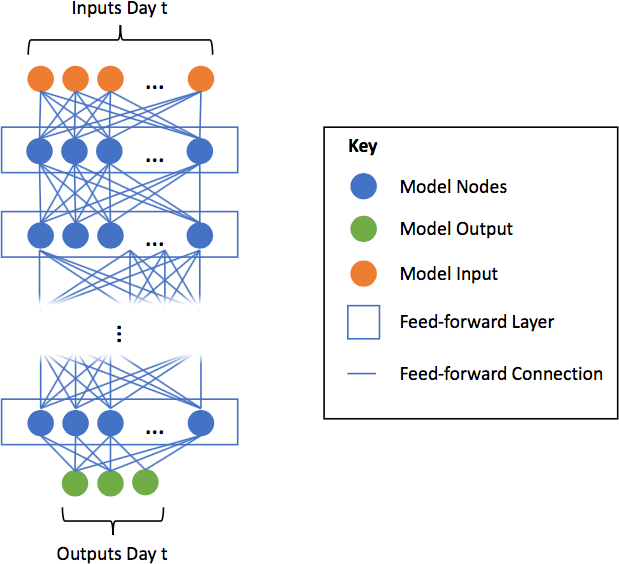
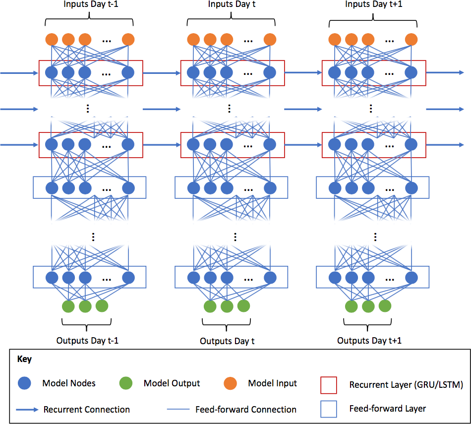
Figure 1. : Example of a Feed-Forward Neural Network (FFNN) for model emulation.

Figure 2. :

Example of a recurrent neural network feeding into FFNN.

4   Experiments

Since DNNs typically require large amounts of data to obtain reliable models [8], we first perform a correlation analysis to ascertain which model runs are sufficiently similar to each other, so that they can be pooled to jointly learn model dynamics. In essence the correlation analysis is used to create clusters of similar model runs.

We compare the outputs of multiple model runs where each model run was conditioned on particular farm management practices, soil types and meteorological outputs from a set of possible scenarios. Each model run also had multiple model outputs and any type of clustering would require that all of these outputs produced sufficiently similar time series. In order to score the level of similarity between model runs, we chose to use a conservative approach that would group two model runs according to the minimum correlation between time series, where the minimum was taken over the individual outputs (runoff, soil_loss, DINrunoff, Nleached). Specifically, we calculated this minimum correlation as $C_{\textup{min}}(i,j)=\min_{k}\textup{Corr}(\mathbf{x}_{i,k},\mathbf{x}_{j,k})$, where $\mathbf{x}_{i,k}$ is the $k$-th model output (eg. soil loss) for model run $i$, while $\textup{Corr}(\cdot)$ represents the sample correlation computed over two vectors.

The correlation function was used to populate symmetric, minimum correlation matrices that can be used to identify clusters. Correlation matrices were produced for each unique combination of meteorology settings, soil type, soil permeability, planting month and planting year, while allowing the management scenario variable to vary. For each correlation matrix, it was then possible to iterate over each row and each column to identify similar model runs across management scenarios that exceeded a minimum correlation threshold (say 0.95).

For both emulation architectures (FFNN and GRU-FFNN), we trialled a range of combinations of hyper-parameters as outlined in Table 4. For the feed-forward parts of the network architecture, we used a funnel shape to the network, whereby the number of nodes in the network decreased with increasing depth. We achieved this by reducing the number of nodes by a half with each layer of depth, starting with the number of nodes listed in Table 4. This conical shape is commonly implemented in FFNN architectures as it helps to reduce the number of parameters/weights in a deep network and can help to facilitate learning that is generalisable rather than simple memorisation of the training data.

Architecture Design Choice	Values Considered
Model Architecture	FFNN, GRU-FFNN
Num. of Lags (days) for Training	7, 14, 28
Num. of Hidden Recurrent Layers	1, 3, 5, 7, 9
Num. of Hidden Feed-Forward Layers	1, 3, 5, 7, 9
Num. of Nodes (Recurrent Layers)	32, 64, 128, 256, 512
Num. of Nodes (Feed-Forward Layers)	32, 64, 128, 256, 512, 1024

Table 2. : Architecture design parameters for DNN based emulators of APSIM outputs.

For training the models, we divided the model runs into three independent, non-overlapping periods in the time series used for: (i) model training (1 Jan 1970 to 31 Dec 2010), (ii) model validation (1 Jan 2011 to 31 Dec 2015), and (iii) model testing (1 Jan 2016 to 19 Nov 2018). The training data was used for training the models in Tensorflow [1] via Keras [3], using the mini-batch Stochastic Gradient Descent algorithm [6]. Training was performed using mini-batches of 128 randomly selected records at a time. In essence, training data was used for updating the weights of the neural network models; validation data was used for assessing overfitting and early stopping; and test data was used for emulator model selection.

We first examined the performance of emulators constructed on clustered data whose minimum correlation across the four output variables was greater than 0.95. Figure 4 visually demonstrates the performance of the FFNN and GRU-FFNN emulators constructed for model runs on one soil type, using clustered data from 3 management classes. Overall, good results were obtained for emulating runoff and DINrunoff, but not for soil_loss and Nleached. In general we found the GRU-FFNN emulator with a moderate number of hidden layers and units per layer (3 layers, 128 units per layer) to be most effective. The FFNN emulator predicts the Nleached variable comparatively poorly.

Emulation via FFNN

 

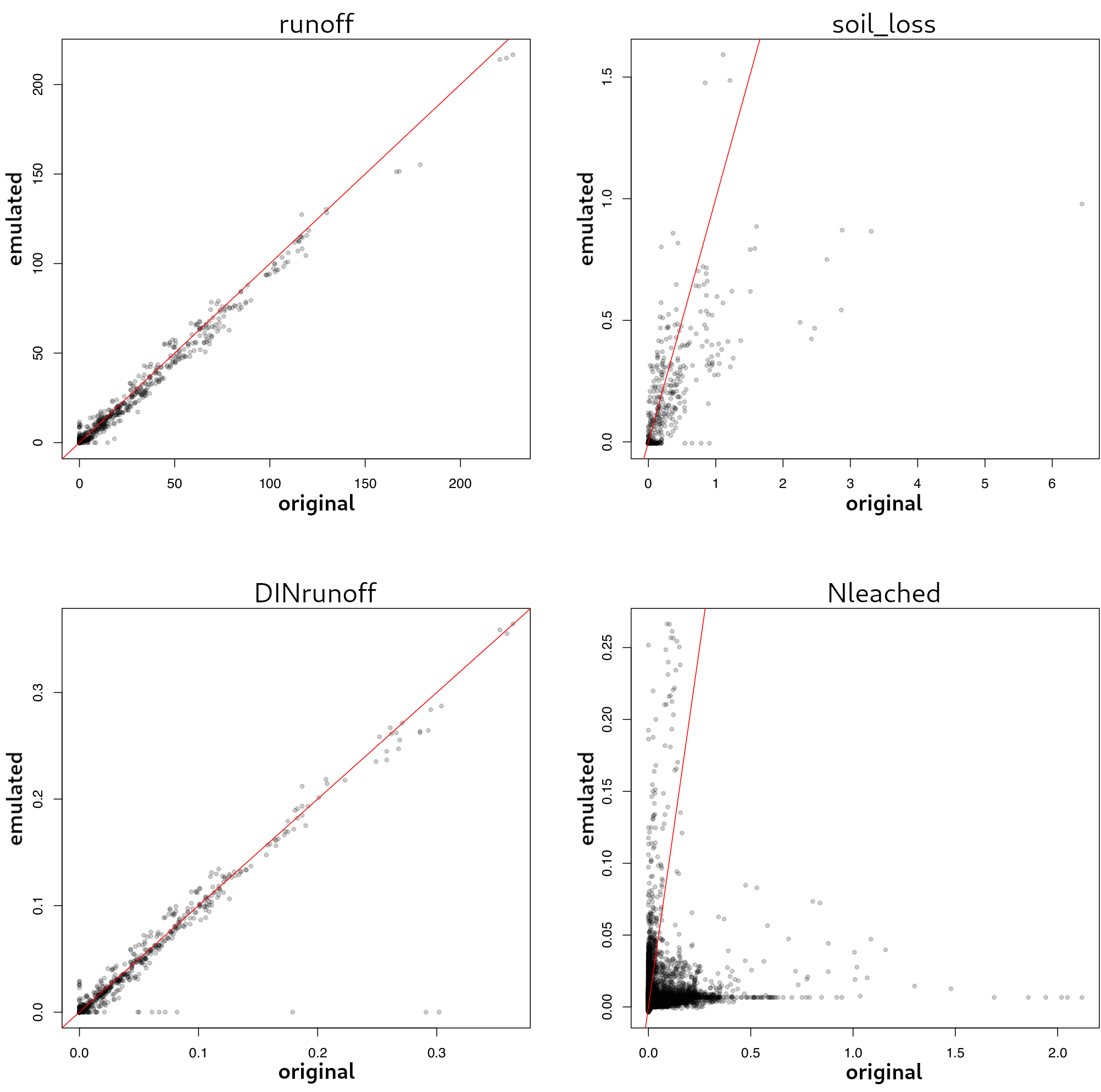
Emulation via GRU-FFNN

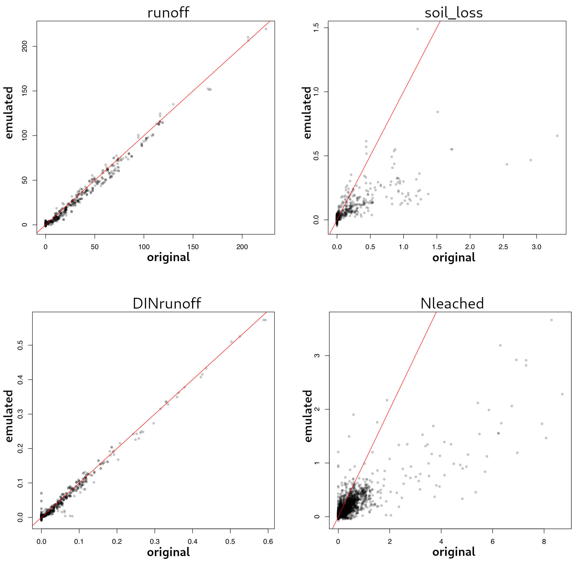
Figure 3. : Scatter plots of APSIM outputs (original) versus emulated outputs for a cluster of model runs with higher than 0.95 correlation. Red lines show equality. Top part: emulation using FFNN with 3 layers containing 128, 64 and 32 units, respectively. Bottom part: emulation using GRU-FFNN with 3 layers and 128 units per layer; corresponding error measures are in Table 4. Plots for soil_loss and Nleached have varying scales to reveal details.

Min. Corr.	Output Variable	MSE	MAE	Bias
Threshold
0.95	runoff	0.612	0.147	-0.0428
	soil_loss	$2.30\times 10^{-3}$	$4.21\times 10^{-3}$	$-3.18\times 10^{-3}$
	DINrunoff	$3.68\times 10^{-6}$	$3.64\times 10^{-4}$	$-1.68\times 10^{-4}$
	Nleached	$4.12\times 10^{-2}$	0.0404	-0.0251
0.90	runoff	0.637	0.135	-0.0446
	soil_loss	$4.19\times 10^{-3}$	$5.82\times 10^{-3}$	$-2.01\times 10^{-3}$
	DINrunoff	$3.11\times 10^{-5}$	$4.70\times 10^{-4}$	$-1.38\times 10^{-4}$
	Nleached	$2.73\times 10^{-3}$	0.0143	$-4.54\times 10^{-3}$
0.85	runoff	0.399	0.120	0.0205
	soil_loss	$5.45\times 10^{-3}$	$5.88\times 10^{-3}$	$-4.11\times 10^{-3}$
	DINrunoff	$3.64\times 10^{-5}$	$4.16\times 10^{-4}$	$-1.35\times 10^{-4}$
	Nleached	$4.82\times 10^{-3}$	0.0197	$-7.39\times 10^{-3}$

Table 3. : Accuracy metrics for 3 layer (128 nodes per layer) GRU-FFNN emulators built using clustered data obtained from various minimum correlation thresholds. MSE: mean squared error. MAE: mean absolute error.

Metrics of emulation accuracy for the GRU-FFNN emulator are listed in Table 4. While the error metrics and biases tend to be small, Figure 4 highlights that some outputs were not emulated well at higher values, and that the small number of these samples (containing such higher values) contribute little to the overall metrics.

With the aim of improving the performance of the emulator, we evaluated lowering the minimum correlation threshold from 0.95 to 0.90 and 0.85, to establish whether more training data might improve the emulation of Nleached and soil_loss. This approach appeared to improve the accuracy of predictions of the Nleached variable, as shown in Table 4. However, in lowering the minimum correlation threshold, we see an undesirable deterioration in the emulation accuracy of the DINrunoff variable (previously well emulated), as well as a slight deterioration in the emulation accuracy of the soil_loss variable (ie. contrary to the desired outcome).

In building emulators from the existing APSIM simulation outputs, the apparent dilemma is that we need more data to train a better model, but in reducing the minimum correlation threshold to admit more data, we are introducing data from other management scenarios that have systematic differences in their dynamics. This suggests that more data (ie. longer time series) is needed from within the same system dynamics (ie. the same management scenarios).

5   Discussion

The obtained results suggest that the opportunistic re-use of existing datasets for developing model emulators of APSIM dynamics is limited to a subset of output variables. Despite large volumes of data in the given dataset of model runs, the dataset has several limitations: sparsity in many of the variables and temporal similarities between various meteorology settings (eg. rain patterns). This suggests that there is limited (and potentially redundant) information in the dataset, which may have hindered training of an accurate emulator.

We hypothesise that the differences in accuracy when predicting the four variables stem from the relative complexity of the relationship between input variables and the outputs. As such, a greater volume of data may be required to adequately learn more complex model dynamics. Interestingly, soil_loss was not emulated well (particularly at higher values), despite the fact that runoff was emulated well and that this would be one of the primary drivers of erosion. This highlights that there are other processes involved in driving soil loss (eg. interactions between runoff and the developmental stage of the cane) that had not been adequately represented in the training dataset.

To develop emulators capable of adequately replicating a wide range of outputs with more complex dynamics, we suggest that a “design of computer experiments” approach [19] should precede the development of emulators, and be used to generate a richer dataset from which the dynamics can be learned. In the context of emulating APSIM models, this can involve sampling a wide variety of combinations of meteorological variables to span the range of all possible inputs to the model.

In particular, we suggest that the next step is to create training data for emulators by feeding a single, very long (say 1000 year), synthetic, randomly generated meteorology file through each of the APSIM scenario files (ie. each combination of farm management conditions and soil type), rather than using meteorology data from a relatively small number of neighbouring regions.

Acknowledgements

We would like to thank the Science Division within the Queensland Government Department of Environment & Science for providing the P2R dataset of APSIM model runs. We would also like to thank Mark Silburn, David Waters, Robin Ellis, Paul Lawrence and Dan Gladish for fruitful discussions. The PyArmadillo library was used for data preparation [18].

References

- [1] M. Abadi, A. Agarwal, P. Barham, E. Brevdo, Z. Chen, C. Citro, G. S. Corrado, A. Davis, J. Dean, et al. TensorFlow: Large-scale machine learning on heterogeneous distributed systems. arXiv:1603.04467, 2016.
- [2] M. J. Asher, B. F. W. Croke, A. J. Jakeman, and L. J. M. Peeters. A review of surrogate models and their application to groundwater modeling. Water Resources Research, 51(8):5957–5973, 2015.
- [3] F. Chollet et al. Keras. https://keras.io, 2015.
- [4] R. R. Curtin, M. Edel, M. Lozhnikov, Y. Mentekidis, S. Ghaisas, and S. Zhang. mlpack 3: a fast, flexible machine learning library. Journal of Open Source Software, 3:726, 2018.
- [5] R. R. Curtin, M. Edel, R. G. Prabhu, S. Basak, Z. Lou, and C. Sanderson. The ensmallen library for flexible numerical optimization. Journal of Machine Learning Research, 22(166):1–6, 2021.
- [6] O. Dekel, R. Gilad-Bachrach, O. Shamir, and L. Xiao. Optimal distributed online prediction using mini-batches. Journal of Machine Learning Research, 13(6):165–202, 2012.
- [7] D. Gladish, D. Pagendam, L. Peeters, P. Kuhnert, and J. Vaze. Emulation engines: choice and quantification of uncertainty for complex hydrological models. Journal of Agricultural, Biological, and Environmental Statistics, 23(1):39–62, 2018.
- [8] I. Goodfellow, Y. Bengio, and A. Courville. Deep Learning. MIT Press, 2016.
- [9] D. P. Holzworth, N. I. Huth, P. G. deVoil, E. J. Zurcher, N. I. Herrmann, G. McLean, K. Chenu, et al. APSIM - evolution towards a new generation of agricultural systems simulation. Environmental Modelling & Software, 62(December):327–350, 2014.
- [10] M. Hooten, W. Leeds, J. Fiechter, and C. Wikle. Assessing first-order emulator inference for physical parameters in nonlinear mechanistic models. Journal of Agricultural, Biological, and Environmental Statistics, 16(4):475–494, 2011.
- [11] M. F. Kasim, D. Watson-Parris, L. Deaconu, S. Oliver, P. Hatfield, D. H. Froula, G. Gregori, M. Jarvis, et al. Building high accuracy emulators for scientific simulations with deep neural architecture search. arXiv:2001.08055v2, 2020.
- [12] M. Kennedy and A. O’Hagan. Bayesian calibration of computer models. Journal of the Royal Statistical Society. Series B: Statistical Methodology, 63(3):425–450, 2001.
- [13] W. Leeds, C. Wikle, J. Fietcher, J. Brown, and R. Milliff. Modeling 3-D spatio-temporal biogeochemical processes with a forest of 1-D statistical emulators. Environmetrics, 24(1):1–12, 2013.
- [14] D. McClymont, D. Freebairn, D. Rattray, J. Robinson, and S. White. Howleaky v5.40.10: Exploring water balance and water quality implication of different land uses. http://www.howleaky.net/, 2011.
- [15] A. Pal, S. Mahajan, and M. Norman. Using deep neural networks as cost-effective surrogate models for super-parameterized E3SM radiative transfer. Geophysical Research Letters, 46(11):6069–6079, 2019.
- [16] A. Paszke, S. Gross, F. Massa, A. Lerer, J. Bradbury, G. Chanan, et al. PyTorch: An imperative style, high-performance deep learning library. In Advances in Neural Information Processing Systems 32, pages 8024–8035, 2019.
- [17] R. Puscasu. Integration of artificial neural networks into operational ocean wave prediction models for fast and accurate emulation of exact nonlinear interactions. Procedia Computer Science, 29:1156–1170, 2014.
- [18] J. Rumengan, T. Y. Zhuo, and C. Sanderson. PyArmadillo: a streamlined linear algebra library for Python. Journal of Open Source Software, 6(66), 2021.
- [19] J. Sacks, J. William, T. Mitchell, and H. Wynn. Design and analysis of computer experiments. Statistical Science, 4(4):409–423, 1989.
- [20] T. J. Santner, B. J. Williams, and W. I. Notz. The Design and Analysis of Computer Experiments. Springer, 2003.
- [21] M. Shaw, M. Silburn, C. Thornton, B. Robinson, and D. McClymont. Modelling pesticide runoff from paddocks in the Great Barrier Reef with HowLeaky. In International Congress on Modelling and Simulation (MODSIM). Modelling and Simulation Society of Australia and New Zealand, 2011.
- [22] M. Sit, B. Z. Demiray, Z. Xiang, G. J. Ewing, Y. Sermet, and I. Demir. A comprehensive review of deep learning applications in hydrology and water resources. Water Science & Technology, 82(12):2635–2670, 2020.