Tensor-network study of correlation-spreading dynamics in the two-dimensional Bose-Hubbard model

Abstract

Recent developments in analog quantum simulators based on cold atoms and trapped ions call for cross-validating the accuracy of quantum-simulation experiments with use of quantitative numerical methods; however, it is particularly challenging for dynamics of systems with more than one spatial dimension. Here we demonstrate that a tensor-network method running on classical computers is useful for this purpose. We specifically analyze real-time dynamics of the two-dimensional Bose-Hubbard model after a sudden quench starting from the Mott insulator by means of the tensor-network method based on infinite projected entangled pair states. Calculated single-particle correlation functions are found to be in good agreement with a recent experiment. By estimating the phase and group velocities from the single-particle and density-density correlation functions, we predict how these velocities vary in the moderate interaction region, which serves as a quantitative benchmark for future experiments and numerical simulations.

I Introduction

State-of-art experimental platforms of cold atoms and trapped ions as analog quantum simulators have offered unique opportunities for studying far-from-equilibrium dynamics of isolated quantum many-body systems. Thanks to their high controllability and long coherence time, these platforms have already addressed a variety of intriguing phenomena that are in general difficult to simulate with classical computers, such as correlation spreading ^{1, 2, 3} and relaxation ^{4, 5, 6} after a quantum quench, many-body localization in a disorder potential ^{7, 8, 9}, and quantum scar states ^{10, 11}. Nevertheless, accurate numerical methods using classical computers are highly demanded at the current stage of the studies of quantum many-body dynamics, since the classical computation still has complementary advantages over the quantum simulation in that it is free of noise and much more accessible owing to its wide dissemination. In this sense, it is important to cross-check the validity of quantum-simulation experiments and some numerical methods by comparing them with each other.

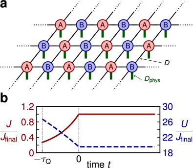
Figure 1: Setup for numerical simulations of quench dynamics. (a) Schematic figure of infinite projected entangled pair state (iPEPS) with a two-site unit cell. Sublattice sites are represented by $A$ and $B$. A rank-five tensor at each site is represented as a circle with four thin lines and one thick line. The former lines correspond to the virtual degrees of freedom with the bond dimension $D$, while the latter line corresponds to the physical degrees of freedom with the dimension of the local Hilbert space $D_{\rm phys}$. The wave functions become more accurate as $D$ increases. (b) Time dependence of the hopping $J$ (a red solid line) and the onsite interaction $U$ (a blue dashed line) with a finite-time quench. The parameter $U/J$ is varied from $\sim 99.4$ to $\sim 19.6$ for $-\tau_{\rm Q}<t<0$ with $\tau_{\rm Q}$ being a finite quench time. In the case of a sudden quench, we discard the region $-\tau_{\rm Q}<t<0$.

In particular, direct comparisons between experimental and numerical outputs have been made for dynamical spreading of two-point spatial correlations of the Bose-Hubbard model ^{1, 3, 12, 13, 14, 15}, which can be realized experimentally with ultracold bosons in optical lattices ¹⁶. The correlation spreading has attracted much theoretical interest ^{17, 18, 12, 19, 20, 21, 22, 13, 14, 23, 24, 15, 25, 26, 27} in the sense that it is closely related to fundamental phenomena, including the propagation of quantum information and the thermalization. In one spatial dimension, quasi-exact numerical methods based on matrix product states (MPSs) have been used to validate the performance of the quantum simulators ^{1, 3, 12}. In two dimensions (2D), by contrast, accurate numerical simulations are challenging. Indeed, the comparisons with respect to a single-particle correlation have shown that a few types of the truncated Wigner approximation (TWA) fail to capture the real-time evolution accurately enough to extract the propagation velocity of the correlation ^{3, 14}. Moreover, while the propagation velocities obtained by a two-particle irreducible strong-coupling (2PISC) approach quantitatively agree with the experimental value, and the approach is applicable to much weaker interaction than in the experiment, it does not necessarily provide the exact value of the correlation itself ¹⁵.

In this paper, we present quantitative numerical analyses of the correlation-spreading dynamics of the 2D Bose-Hubbard model starting from a Mott insulating initial state with unit filling. To this end, we employ the tensor-network method based on the infinite projected entangled pair state (iPEPS) ^{28, 29, 30, 31, 32, 33, 34, 35} or the tensor product state ^{36, 37, 38, 39, 40}, which is an extension of MPS to 2D systems [see Fig.1(a)]. The iPEPS studies on real-time dynamics of isolated ^{41, 42, 43, 44, 45, 46, 47, 48, 49} and open ^{41, 42, 50, 51, 52} quantum systems in 2D have begun very recently. Previous simulations suggest that iPEPS can represent relatively low-entangled states in short-time dynamics for simple spin $1/2$ systems ^{41, 42, 43, 44} and some itinerant electron systems ⁴⁶. This observation may be valid for real-time dynamics in Bose-Hubbard systems; however, little is known about it until now. We find that the single-particle correlation computed with iPEPS, as well as the estimated propagation velocity of the correlation front, agrees very well with the experimental result ³, demonstrating that iPEPS can be useful for actual quantum-simulation experiments. We also conduct numerical simulations in a moderate interaction region, which has not been addressed by the previous experiments ^{1, 3}. From the real-time evolution of the single-particle and density-density correlations, we show that the phase and group velocities approach each other when the interaction decreases.

II Results

II.1 Model

We consider the Bose-Hubbard model on a square lattice ^{53, 54}. The Hamiltonian is given as

$$\hat{H}=-J\sum_{\langle ij\rangle}(\hat{a}^{\dagger}_{i}\hat{a}_{j}+\hat{a}^{\dagger}_{j}\hat{a}_{i})+\frac{U}{2}\sum_{i}\hat{n}_{i}(\hat{n}_{i}-1)-\mu\sum_{i}\hat{n}_{i},$$ (1)

where $\hat{a}^{\dagger}_{i}$ and $\hat{a}_{i}$ are the creation and annihilation operators at site $i$, $\hat{n}_{i}=\hat{a}^{\dagger}_{i}\hat{a}_{i}$ is the number operator, $J$ is the strength of the hopping between nearest-neighbor sites, $U$ is the strength of the onsite interaction, and $\mu$ is the chemical potential. The notation $\langle ij\rangle$ indicates that sites $i$ and $j$ are nearest neighbors. For simplicity, we ignore the effects of the trap potential and the Gaussian envelopes of optical lattice lasers, which do not affect short-time dynamics. We set the lattice spacing $d_{\rm lat}$ to be unity. The ground state at the commensurate filling is the Mott insulating (superfluid) state for $U\gg J$ ($U\ll J$). Hereafter, we will consider a sudden quench and a quench with a short time [see Fig. 1(b) and Supplementary Note 1 for details].

II.2 Quench starting from the Mott insulator: Comparison with the exact diagonalization and the experiment

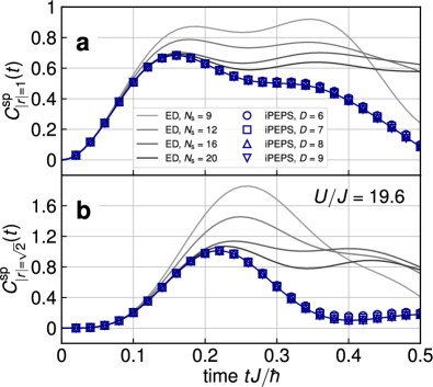
Figure 2: Single-particle correlation functions $C^{\rm sp}_{\bm{r}}(t)$ in the case of a sudden quench. Comparison is made between the infinite projected entangled pair state algorithm (iPEPS, blue lines with symbols) and the exact diagonalization method (ED, gray lines). The unit of time is taken as the inverse of the strength of the hopping $J$. $U$ is the strength of the interaction. $D$ is the bond dimension. $N_{\rm s}$ is the system size. The correlations at distances (a) $|\bm{r}|=1$ and (b) $|\bm{r}|=\sqrt{2}$ are shown. Both results overlap in a short time.

Let us first focus on the case of a sudden quench. We compare our results of iPEPS with those of the exact diagonalization (ED) method and obtain consistent results in a short time. In the ED simulations using the QuSpin library ^{55, 56}, we choose the system sizes $L_{x}\times L_{y}$ up to $5\times 4$ and use the periodic-periodic boundary condition. We examine to what extent the energy is conserved in the iPEPS simulations. The grand potential density $\langle\hat{H}\rangle$ at $T=0$ starting from the Mott insulator $\otimes_{i}|n_{i}=1\rangle$ should remain constant. They well converge for the bond dimensions $D\geq 6$ and remain nearly constant up to $t\sim 0.4\hbar/J$ (see Supplementary Note 2 for the time dependence of the grand potential density). We also investigate how the single-particle correlations converge with increasing bond dimensions. The equal-time single-particle correlation function at a distance $\bm{r}=(x,y)$ for the system size $N_{\rm s}$ is defined as

$$C^{\rm sp}_{\bm{r}}(t)=\frac{1}{2N_{\rm s}}\sum_{i,j}{\vphantom{\sum}}^{\prime}\langle\hat{a}^{\dagger}_{i}(t)\hat{a}_{j}(t)+\hat{a}^{\dagger}_{j}(t)\hat{a}_{i}(t)\rangle.$$ (2)

Here $\sum_{i,j}^{\prime}$ denotes the summation over $(i,j)$ that satisfies $|x_{j}-x_{i}|=x$ and $|y_{j}-y_{i}|=y$. In the iPEPS simulations, $1/N_{\rm s}\times\sum_{i,j}^{\prime}$ is replaced by $1/2\times\sum_{i=A,B}\sum_{j}^{\prime}$ with $A$ and $B$ being sublattice sites because of the translational invariance. As shown in Fig. 2, $C^{\rm sp}_{|\bm{r}|=1}(t):=[C^{\rm sp}_{\bm{r}=(1,0)}(t)+C^{\rm sp}_{\bm{r}=(0,1)}(t)]/2$ exhibits a peak at $t\sim 0.15\hbar/J$ in both results, and they overlap in this short time. For $t\gtrsim 0.15\hbar/J$, the correlation functions of ED start to exhibit a significant finite-size effect, whereas those of iPEPS converge for $D\geq 6$. We observe similar behavior for $C^{\rm sp}_{|\bm{r}|=\sqrt{2}}(t):=C^{\rm sp}_{\bm{r}=(1,1)}(t)$. The iPEPS results are better simulated up to a longer time (see also Supplementary Note 3 for other interaction parameter regions).

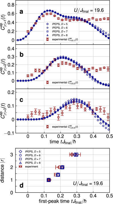
Figure 3: Single-particle correlation functions $C^{\rm sp}_{\bm{r}}(t)$ in the case of a finite-time quench. Comparison is made between the infinite projected entangled pair state algorithm (iPEPS, blue lines with symbols) and the experiment (red circles with error bars). The unit of time is taken as the inverse of the strength of the hopping $J_{\rm final}$ after the quench. $U$ is the strength of the interaction. $D$ is the bond dimension. The correlations at distances (a) $|\bm{r}|=1$, (b) $|\bm{r}|=2$, and (c) $|\bm{r}|=3$ are shown. The error bars represent the standard error of five independent measurements ³. (d) Comparison of the first-peak time between the iPEPS and experimental results. The error bars represent the fitting errors ³. The iPEPS and experimental results agree within the experimental errors in all cases.

Next, we compare the correlations of iPEPS with those of the experiment ³ for a finite quench time. In the experiment, a quench to the Mott insulating region has been investigated so far. Figures 3(a–c) show the time evolution of correlations at distances $|\bm{r}|=1$, $2$, and $3$, respectively. Qualitative behavior is essentially equivalent to the case of the sudden quench, although the correlation function shifts to an earlier time. For $|\bm{r}|=1$, both data show a peak at $t\sim 0.12\hbar/J_{\rm final}$. Similarly, the first-peak times are consistent with each other for $|\bm{r}|=2$ and $3$, and they become longer with increasing distances. When the energy is approximately conserved (namely, for $t\lesssim 0.4\hbar/J_{\rm final}$, see the time dependence of the grand potential density in Supplementary Note 4), the intensities of correlations also overlap very well. They are also consistent with those obtained by TWA ^{13, 3, 14}, while the iPEPS simulations can deal with a slightly longer time and capture the correlation peaks more clearly (see also Supplementary Note 5 for a detailed comparison with the TWA results). To see how well they match more quantitatively, we also compare the first-peak position of iPEPS with that of the experiment ³ as shown in Fig. 3(d). Both iPEPS and experimental results agree very well.

II.3 Estimates of group and phase velocities in the moderate interaction region

Having confirmed the applicability of iPEPS simulations to real-time evolution of the Bose-Hubbard model, we study how information propagates by a sudden quench in the moderate interaction region. There are two kinds of velocity that are relevant to the correlation spreading. One is the group velocity $v_{\rm gr}$, which corresponds to the propagation of the envelope of the wave packet and is a suitable quantity to characterize the spreading of correlations. In non-relativistic quantum many-body systems, $v_{\rm gr}$ is bounded above, and the upper bound is known as the Lieb-Robinson bound ^{57, 58, 23, 24, 25, 26, 27}. Notice that the Lieb-Robinson bound for the Bose-Hubbard model has not been rigorously derived with a few exceptions for limited situations ^{18, 23, 24, 25, 26, 27}. The phase velocity $v_{\rm ph}$ is the other characteristic quantity, which corresponds to the propagation of the first peak of the wave packet, and does not have to obey the Lieb-Robinson bound.

Although the exact Lieb-Robinson bound is not known for the Bose-Hubbard model, there are some values that can be used as a guide. As discussed in previous studies ^{1, 3, 12} in the weak interaction region, the single-particle dispersion up to constant is approximately given as $\epsilon_{U\ll J}(\bm{k})\sim-2J\sum_{\alpha}\cos k_{\alpha}$ ($\alpha=x,y$ in 2D), which is equivalent to the dispersion of free particles. The velocity of the correlation spreading would be well characterized by the group velocity of the single-particle excitation. The largest velocity of a single quasiparticle (along the horizontal or vertical direction $\alpha$) is described by the maximal slope of the dispersion and is given by $v=\max_{k_{\alpha}}[d|\epsilon_{U\ll J}(\bm{k})|/dk_{\alpha}]/\hbar=2J/\hbar$. Because both doublon and holon quasiparticles propagate with the group velocity $v$, the front of the correlation function moves at the speed of $v_{\rm front}$, which should be smaller than $v_{\rm max}=2v=4J/\hbar$. Therefore, this speed $v_{\rm max}$ can be regarded as the Lieb-Robinson-bound-like value. Likewise, in the strong interaction region, the doublon and holon dispersions up to constant are approximately given as $\epsilon^{(d)}_{U\gg J}(\bm{k})\sim-4J\sum_{\alpha}\cos k_{\alpha}$ and $\epsilon^{(h)}_{U\gg J}(-\bm{k})\sim-2J\sum_{\alpha}\cos k_{\alpha}$, respectively. Because the doublons and holons propagate with respective velocities $4J/\hbar$ and $2J/\hbar$, $v_{\rm front}$ should be smaller than these two sum $v_{\rm max}=6J/\hbar$. Although we know the approximate limit values, the intermediate interaction region is yet to be explored.

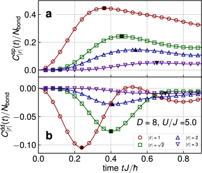
Figure 4: Single particle and density-density correlation functions used to extract the propagation velocities. (a) Single-particle [$C^{\rm sp}_{\bm{r}}(t)$] and (b) density-density [$C^{\rm dd}_{\bm{r}}(t)$] correlation functions per bond at the interaction strength $U/J=5$ for the bond dimension $D=8$. The unit of time is taken as the inverse of the strength of the hopping $J$. The normalization factor at a distance $\bm{r}=(x,y)$ is given as $N_{\rm bond}=2$ for $x\not=y$ ($|\bm{r}|=1$, $2$, and $3$), while it is $N_{\rm bond}=4$ for $x=y$ ($|\bm{r}|=\sqrt{2}$). The black symbol corresponds to the first peak in the correlation function obtained by cubic spline interpolation of data points. The propagation velocities along the horizontal or vertical axis are extracted by the data at $|\bm{r}|=1$, $2$, and $3$. The velocity estimated from the density-density correlation functions is slower than that from the single-particle correlation functions.

To estimate the group velocity from the single-particle correlations, long-time simulations are required in general. However, it is challenging in the iPEPS simulations. To circumvent the difficulty, we estimate the group velocity by the density-density correlation. It is known that the propagation velocity of the first peak of this correlation agrees very well with the group velocity ^{1, 12}. The equal-time density-density correlation function at a distance $\bm{r}=(x,y)$ for the system size $N_{\rm s}$ is defined as

$$C^{\rm dd}_{\bm{r}}(t)=\frac{1}{N_{\rm s}}\sum_{i,j}{\vphantom{\sum}}^{\prime}\langle\hat{n}_{i}(t)\hat{n}_{j}(t)\rangle_{\rm c},$$ (3)

where $\langle\cdots\rangle_{\rm c}$ denotes a connected correlation function. In our simulations, $\langle\hat{n}_{i}(t)\hat{n}_{j}(t)\rangle_{\rm c}=\langle\hat{n}_{i}(t)\hat{n}_{j}(t)\rangle-1$ because $\langle\hat{n}_{i}(t)\rangle=1$ for all sites and time steps. As in $C^{\rm sp}_{\bm{r}}(t)$, the summation is replaced by that within sublattice sites in the iPEPS simulations. The parity-parity correlation closely related to the density-density one can be measured in experiments by using the quantum-gas microscope techniques ¹.

We extract the propagation velocities from the first peak in both correlations for $|{\bm{r}}|=1$, $2$, and $3$. For simplicity, we consider the sudden quench hereafter. When the interaction becomes weaker, we have confirmed that the energy is conserved in a longer time frame; typically, $t\lesssim 0.9\hbar/J$ for $U/J\sim 5$ (see Supplementary Note 6 for the time dependence of the grand potential density in the weaker interaction region). All the correlation peaks for $|\bm{r}|\leq 3$ appear in this time frame (see Fig. 4). The first peak of the single-particle correlation appears at $t\sim 0.35\hbar/J$ for $|\bm{r}|=1$, while it appears at $t\sim 0.65\hbar/J$ for $|\bm{r}|=3$. By contrast, the first peak of the density-density correlation appears at $t\sim 0.25\hbar/J$ for $|\bm{r}|=1$, while it appears at $t\sim 0.7\hbar/J$ for $|\bm{r}|=3$. It takes a long time for propagation in the latter case. (See also the correlations for other interaction parameters given in Supplementary Note 7. Extraction of propagation velocities in the intermediate and strong interaction regions is summarized in Supplementary Notes 8 and 9, respectively.) The first-peak time is almost a linear function of the distance, and the system exhibits the light-cone-like spreading of correlations (see the time dependence of distance summarized in Supplementary Note 8).

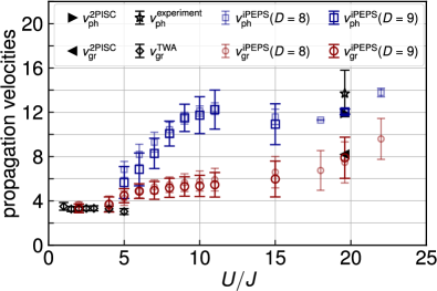
Figure 5: Propagation velocities as functions of the ratio between the interaction ($U$) and hopping ($J$) strengths. The group ($v_{\rm gr}$, red circles) and phase ($v_{\rm ph}$, blue squares) velocities are estimated from the density-density and single-particle correlation functions for the bond dimensions $D=8$ and $D=9$ using the infinite projected entangled pair state (iPEPS) algorithm. The data for $D=8$ and $D=9$ overlap within the error bars. The velocities and their error bars are obtained by extrapolation of the distance dependence of the peak time. The results obtained by the two-particle irreducible strong-coupling (2PISC) approach ¹⁵ (triangles), the truncated Wigner approximation (TWA) ¹³ (diamonds), and the experiment ³ (a star) are shown. Both velocities gradually merge with decreasing interaction.

We summarize the interaction dependence of the group and phase velocities in Fig. 5. In the weak interaction region, the estimated group velocities are $v_{\rm gr}\sim 4J/\hbar$. They are similar to those obtained by the TWA at filling factor $\nu=10$ ¹³. They are also consistent with the group velocity $v_{\rm gr}(U=0)=4J/\hbar$ of a single particle ¹³. In the strong interaction region, the estimated group velocity $v_{\rm gr}\sim(8\pm 2)J/\hbar$ at $U/J=19.6$ coincides with that obtained by the 2PISC approach ¹⁵ within the error bar of extrapolation. It is also comparable to the group velocity $v_{\rm gr}(U\gg J)=6J/\hbar\times[1+\mathcal{O}(J^{2}/U^{2})]$ of a quasi-particle in the large $U$ limit ^{1, 12, 3}. Similarly, the estimated phase velocity agrees very well with the results of the 2PISC approach ¹⁵ and the experiment ³. In the intermediate region, the estimated group velocity is closer to the single-particle group velocity in the superfluid region, whereas it is comparable to the 2PISC result near and above the critical point $U_{\rm c}/J\sim 16.7$ ^{59, 60, 61}.

In all parameter regions, no anomalies appear in the propagation velocities. As for the real-time dynamics after a sudden quench, there is no sign of the superfluid-Mott insulator quantum phase transition. This is because non-universal high-energy excitations come into play during the time evolution. The quantum phase transition at zero temperature does not have to affect the time-evolved states.

Both group and phase velocities gradually converge to the same value as $U/J$ is decreased. This phenomenon can be understood in terms of the separation of the energy scales. When the interaction $U$ is much stronger than the hopping $J$, the correlation function oscillates rapidly as a function of time ^{12, 22}. The correlation function exhibits the envelope of the wave packet. The time scale of the period of oscillation is $\sim 1/U$, which determines the phase velocity $v_{\rm ph}\sim U$. On the other hand, the time scale of the period of the envelope is $\sim 1/J$, which determines the group velocity $v_{\rm gr}\sim J$. Hence, the group and phase velocities differ as long as $U\gg J$. When the interaction $U$ becomes comparable to the hopping $J$, they start to coincide by slowing down the vibration. Note that this phenomenon occurs irrespective of the presence or absence of phase transitions.

III Conclusions

We have studied real-time dynamics of the 2D Bose-Hubbard model after a sudden quench starting from the Mott insulator with unit filling. We have employed the 2D tensor-network method based on the iPEPSs, which are the 2D extension of the well-known MPSs in one dimension. Calculated single-particle correlation functions reproduce the recent experimental results very well. The iPEPS algorithm can simulate real-time dynamics long enough for extracting the propagation velocities from correlations. This fact suggests that, for the quench dynamics starting from the Mott insulator in the 2D Bose-Hubbard model, time-evolved states are not so highly entangled before and even slightly after the time at which the correlation front is reached. This finding raises questions about our understanding of how quantum states get entangled with real-time evolution.

We have also estimated the group and phase velocities in the moderate interaction region, in which the 2PISC approach and the TWA are not applicable. The estimated group velocities are continuously connected without singularity in the middle. Our findings would be useful in the future analog quantum simulation and in the future examination of the rigorous Lieb-Robinson bound of Bose-Hubbard systems. The ability of the tensor-network method that accurately calculates the real-time dynamics of 2D quantum many-body systems opens up the possibility of applying it to other quantum-simulation platforms, such as Rydberg atoms, trapped ions, and superconducting circuits.

IV Methods

IV.1 Real-time evolution by infinite projected entangled pair states

We prepare iPEPS with a two-site unit cell [see Fig. 1(a)]. The symbols $D$ and $D_{\rm phys}$ denote the virtual bond dimension and the dimension of the local Hilbert space, respectively. The former improves the accuracy of the wave function, whereas the latter corresponds to the maximum particle number $n_{\rm max}$ as $D_{\rm phys}=n_{\rm max}+1$. Although $n_{\rm max}$ can take infinity in Bose-Hubbard systems, it is practically bounded above in the presence of interaction ^{62, 63}. We can choose finite $D_{\rm phys}$ in the simulations of real-time dynamics. In the case of a sudden quench to the Mott insulating region ($U/J>U_{\rm c}/J\sim 16.7$ ^{59, 60, 61}), we set the dimension of the local Hilbert space as $D_{\rm phys}=3$ because the number of particles deviates only slightly from unity ^{62, 63}. For $U/J<U_{\rm c}/J$, we choose $D_{\rm phys}=5$ so that the wave functions can further take into account the effect of particle fluctuations. When $U$ is close to zero (at $U/J=2$ in our simulations), we use slightly larger $D_{\rm phys}=7$ (see Supplementary Note 10 for the details of the choice of the dimensions of the local Hilbert space). The initial Mott insulating state $\otimes_{i}|n_{i}=1\rangle$ can be represented with the bond dimension $D=1$. As for static properties, the Bose-Hubbard model was investigated by finite PEPS or iPEPS, and the phase transition between the Mott insulating and superfluid phases was reproduced ^{64, 65, 66, 67, 68, 69, 70, 71, 72}.

The wave function at each time $|\Psi(t)\rangle=e^{-it\hat{H}/\hbar}|\Psi(0)\rangle$ is obtained by real-time evolving iPEPS ^{41, 42, 43}. The real-time evolution operator in a small time step $dt$ can be approximated by the Suzuki-Trotter decomposition ^{73, 74, 75} as $e^{-idt\hat{H}/\hbar}\sim\prod_{\langle ij\rangle}e^{-idt\hat{H}_{ij}/\hbar}$, where $\hat{H}_{ij}=-J(\hat{a}^{\dagger}_{i}\hat{a}_{j}+\hat{a}^{\dagger}_{j}\hat{a}_{i})+U[\hat{n}_{i}(\hat{n}_{i}-1)+\hat{n}_{j}(\hat{n}_{j}-1)]/(2z)-\mu(\hat{n}_{i}+\hat{n}_{j})/z$ with the coordination number $z=4$ is the local Hamiltonian satisfying $\hat{H}=\sum_{\langle ij\rangle}\hat{H}_{ij}$. After applying the two-site gate $e^{-idt\hat{H}_{ij}/\hbar}$ to neighboring tensors, we approximate the local tensors by the singular value decomposition in such a way that the virtual bond dimension of iPEPS remains $D$. In the actual simulations, the second-order Suzuki-Trotter decomposition is used for this simple update algorithm ^{76, 32}, and the tensor-network library TeNeS ^{77, 78, 79} is adopted. The wave functions are optimized up to the bond dimension $D=9$. Qualitative behavior of correlation functions is found to be nearly the same for $D\geq 6$. When extracting the propagation velocities, we mainly use the data for $D=8$ and $D=9$ to ensure sufficient convergence of physical quantities. We do not preserve the $\rm U(1)$ symmetry during the calculation. Even without respecting the symmetry, we have numerically found that at these values of $D$, the number of particles is nearly conserved during the real-time evolution starting from the Mott insulator.

Physical quantities in the thermodynamic limit are calculated by the corner transfer matrix renormalization group (CTMRG) method ^{80, 81, 82, 37, 83, 84, 85, 86, 33, 34, 35}. The bond dimension of the environment tensors is chosen as $\chi=2D^{2}$ to ensure that physical quantities are well converged.

To compare our results obtained by iPEPS with the experiment ³, we consider a quench with a short time $\tau_{\rm Q}=0.1\mathrm{ms}$ ^{13, 14} [see Fig. 1(b)]. For $-\tau_{\rm Q}<t<0$, both $J$ and $U$ are controlled. The wave function is updated as $|\Psi(t+dt)\rangle\sim e^{-idt\hat{H}(t)/\hbar}|\Psi(t)\rangle$ with the time-dependent Hamiltonian $\hat{H}(t)$ in this region. For $t>0$, both parameters are fixed. We take $J_{\rm final}=J(t=0)\sim 0.0612\hbar/\tau_{\rm Q}$ as the unit of energy. The discrete time step for the real-time evolution is set to be $dt/(\hbar/J_{\rm final})=\tau_{\rm Q}/(\hbar/J_{\rm final})/15\sim 0.00408$ for all $t$. To compare the iPEPS results with the exact real-time dynamics in finite-size systems, we also consider a sudden parameter change and set the time step as $dt/(\hbar/J)=0.005$. We have checked that the simulations with doubled and halved $dt$ do not change the results significantly.

V Data availability

The data obtained by the iPEPS and ED simulations in this paper are available at https://doi.org/10.5281/zenodo.6085592. The experimental data ³ and the data obtained by the TWA simulations ¹³ in this paper are available from the authors upon request.

VI Code availability

The codes in this paper are available from the authors upon request.

VII Author contributions

R.K. and I.D. designed and coordinated the studies. R.K. performed the numerical simulations. R.K. and I.D. contributed to the writing of the paper.

VIII Competing interests

The authors declare no competing interests.

IX Additional information

Supplementary Information The online version contains supplementary material available at https://doi.org/10.1038/s42005-022-00848-9.

References

- Cheneau et al. [2012] M. Cheneau, P. Barmettler, D. Poletti, M. Endres, P. Schauß, T. Fukuhara, C. Gross, I. Bloch, C. Kollath, and S. Kuhr, Light-cone-like spreading of correlations in a quantum many-body system, Nature 481, 484 (2012).
- Jurcevic et al. [2014] P. Jurcevic, B. P. Lanyon, P. Hauke, C. Hempel, P. Zoller, R. Blatt, and C. F. Roos, Quasiparticle engineering and entanglement propagation in a quantum many-body system, Nature 511, 202 (2014).
- Takasu et al. [2020] Y. Takasu, T. Yagami, H. Asaka, Y. Fukushima, K. Nagao, S. Goto, I. Danshita, and Y. Takahashi, Energy redistribution and spatio-temporal evolution of correlations after a sudden quench of the Bose-Hubbard model, Sci. Adv. 6, eaba9255 (2020).
- Trotzky et al. [2012] S. Trotzky, Y.-A. Chen, A. Flesch, I. P. McCulloch, U. Schollwöck, J. Eisert, and I. Bloch, Probing the relaxation towards equilibrium in an isolated strongly correlated one-dimensional Bose gas, Nat. Phys. 8, 325 (2012).
- Langen et al. [2015] T. Langen, S. Erne, R. Geiger, B. Rauer, T. Schweigler, M. Kuhnert, W. Rohringer, I. E. Mazets, T. Gasenzer, and J. Schmiedmayer, Experimental observation of a generalized Gibbs ensemble, Science 348, 207 (2015).
- Kaufman et al. [2016] A. M. Kaufman, M. E. Tai, A. Lukin, M. Rispoli, R. Schittko, P. M. Preiss, and M. Greiner, Quantum thermalization through entanglement in an isolated many-body system, Science 353, 794 (2016).
- Schreiber et al. [2015] M. Schreiber, S. S. Hodgman, P. Bordia, H. P. Lüschen, M. H. Fischer, R. Vosk, E. Altman, U. Schneider, and I. Bloch, Observation of many-body localization of interacting fermions in a quasirandom optical lattice, Science 349, 842 (2015).
- Choi et al. [2016] J.-y. Choi, S. Hild, J. Zeiher, P. Schauß, A. Rubio-Abadal, T. Yefsah, V. Khemani, D. A. Huse, I. Bloch, and C. Gross, Exploring the many-body localization transition in two dimensions, Science 352, 1547 (2016).
- Smith et al. [2016] J. Smith, A. Lee, P. Richerme, B. Neyenhuis, P. W. Hess, P. Hauke, M. Heyl, D. A. Huse, and C. Monroe, Many-body localization in a quantum simulator with programmable random disorder, Nat. Phys. 12, 907 (2016).
- Bernien et al. [2017] H. Bernien, S. Schwartz, A. Keesling, H. Levine, A. Omran, H. Pichler, S. Choi, A. S. Zibrov, M. Endres, M. Greiner, V. Vuletić, and M. D. Lukin, Probing many-body dynamics on a 51-atom quantum simulator, Nature 551, 579 (2017).
- Turner et al. [2018] C. J. Turner, A. A. Michailidis, D. A. Abanin, M. Serbyn, and Z. Papić, Weak ergodicity breaking from quantum many-body scars, Nat. Phys. 14, 745 (2018).
- Barmettler et al. [2012] P. Barmettler, D. Poletti, M. Cheneau, and C. Kollath, Propagation front of correlations in an interacting Bose gas, Phys. Rev. A 85, 053625 (2012).
- Nagao et al. [2019] K. Nagao, M. Kunimi, Y. Takasu, Y. Takahashi, and I. Danshita, Semiclassical quench dynamics of Bose gases in optical lattices, Phys. Rev. A 99, 023622 (2019).
- Nagao et al. [2021] K. Nagao, Y. Takasu, Y. Takahashi, and I. Danshita, SU(3) truncated Wigner approximation for strongly interacting Bose gases, Phys. Rev. Research 3, 043091 (2021).
- Mokhtari-Jazi et al. [2021] A. Mokhtari-Jazi, M. R. C. Fitzpatrick, and M. P. Kennett, Phase and group velocities for correlation spreading in the Mott phase of the Bose-Hubbard model in dimensions greater than one, Phys. Rev. A 103, 023334 (2021).
- Greiner et al. [2002] M. Greiner, O. Mandel, T. Esslinger, T. W. Hänsch, and I. Bloch, Quantum phase transition from a superfluid to a Mott insulator in a gas of ultracold atoms, Nature 415, 39 (2002).
- Läuchli and Kollath [2008] A. M. Läuchli and C. Kollath, Spreading of correlations and entanglement after a quench in the one-dimensional Bose–Hubbard model, J. Stat. Mech. Theory Exp. 2008, P05018 (2008).
- Schuch et al. [2011] N. Schuch, S. K. Harrison, T. J. Osborne, and J. Eisert, Information propagation for interacting-particle systems, Phys. Rev. A 84, 032309 (2011).
- Carleo et al. [2014] G. Carleo, F. Becca, L. Sanchez-Palencia, S. Sorella, and M. Fabrizio, Light-cone effect and supersonic correlations in one- and two-dimensional bosonic superfluids, Phys. Rev. A 89, 031602(R) (2014).
- Cevolani et al. [2018] L. Cevolani, J. Despres, G. Carleo, L. Tagliacozzo, and L. Sanchez-Palencia, Universal scaling laws for correlation spreading in quantum systems with short- and long-range interactions, Phys. Rev. B 98, 024302 (2018).
- Fitzpatrick and Kennett [2018] M. R. C. Fitzpatrick and M. P. Kennett, Light-cone-like spreading of single-particle correlations in the Bose-Hubbard model after a quantum quench in the strong-coupling regime, Phys. Rev. A 98, 053618 (2018).
- Despres et al. [2019] J. Despres, L. Villa, and L. Sanchez-Palencia, Twofold correlation spreading in a strongly correlated lattice Bose gas, Sci. Rep. 9, 4135 (2019).
- Wang and Hazzard [2020] Z. Wang and K. R. A. Hazzard, Tightening the Lieb-Robinson Bound in Locally Interacting Systems, PRX Quantum 1, 010303 (2020).
- Kuwahara and Saito [2021] T. Kuwahara and K. Saito, Lieb-Robinson Bound and Almost-Linear Light Cone in Interacting Boson Systems, Phys. Rev. Lett. 127, 070403 (2021).
- [25] C. Yin and A. Lucas, Finite speed of quantum information in models of interacting bosons at finite density, arXiv:2106.09726 .
- Faupin et al. [a] J. Faupin, M. Lemm, and I. M. Sigal, On Lieb-Robinson bounds for the Bose-Hubbard model, arXiv:2109.04103 .
- Faupin et al. [b] J. Faupin, M. Lemm, and I. M. Sigal, Maximal speed for macroscopic particle transport in the Bose-Hubbard model, arXiv:2110.04313 .
- Martín-Delgado et al. [2001] M. A. Martín-Delgado, M. Roncaglia, and G. Sierra, Stripe ansätze from exactly solved models, Phys. Rev. B 64, 075117 (2001).
- [29] F. Verstraete and J. I. Cirac, Renormalization algorithms for quantum-many body systems in two and higher dimensions, arXiv:cond-mat/0407066 .
- Verstraete and Cirac [2004] F. Verstraete and J. I. Cirac, Valence-bond states for quantum computation, Phys. Rev. A 70, 060302(R) (2004).
- Verstraete et al. [2008] F. Verstraete, V. Murg, and J. I. Cirac, Matrix product states, projected entangled pair states, and variational renormalization group methods for quantum spin systems, Adv. Phys. 57, 143 (2008).
- Jordan et al. [2008] J. Jordan, R. Orús, G. Vidal, F. Verstraete, and J. I. Cirac, Classical Simulation of Infinite-Size Quantum Lattice Systems in Two Spatial Dimensions, Phys. Rev. Lett. 101, 250602 (2008).
- Phien et al. [2015] H. N. Phien, J. A. Bengua, H. D. Tuan, P. Corboz, and R. Orús, Infinite projected entangled pair states algorithm improved: Fast full update and gauge fixing, Phys. Rev. B 92, 035142 (2015).
- Orús [2014] R. Orús, A practical introduction to tensor networks: Matrix product states and projected entangled pair states, Ann. Phys. (N.Y.) 349, 117 (2014).
- Orús [2019] R. Orús, Tensor networks for complex quantum systems, Nat. Rev. Phys. 1, 538 (2019).
- Hieida et al. [1999] Y. Hieida, K. Okunishi, and Y. Akutsu, Numerical renormalization approach to two-dimensional quantum antiferromagnets with valence-bond-solid type ground state, New J. Phys. 1, 7 (1999).
- Okunishi and Nishino [2000] K. Okunishi and T. Nishino, Kramers-Wannier approximation for the 3D Ising model, Prog. Theor. Phys. 103, 541 (2000).
- Nishino et al. [2001] T. Nishino, Y. Hieida, K. Okunishi, N. Maeshima, Y. Akutsu, and A. Gendiar, Two-dimensional tensor product variational formulation, Prog. Theor. Phys. 105, 409 (2001).
- Maeshima et al. [2001] N. Maeshima, Y. Hieida, Y. Akutsu, T. Nishino, and K. Okunishi, Vertical density matrix algorithm: A higher-dimensional numerical renormalization scheme based on the tensor product state ansatz, Phys. Rev. E 64, 016705 (2001).
- [40] Y. Nishio, N. Maeshima, A. Gendiar, and T. Nishino, Tensor product variational formulation for quantum systems, arXiv:cond-mat/0401115 .
- Kshetrimayum et al. [2017] A. Kshetrimayum, H. Weimer, and R. Orús, A simple tensor network algorithm for two-dimensional steady states, Nat. Commun. 8, 1 (2017).
- Czarnik et al. [2019] P. Czarnik, J. Dziarmaga, and P. Corboz, Time evolution of an infinite projected entangled pair state: An efficient algorithm, Phys. Rev. B 99, 035115 (2019).
- Hubig and Cirac [2019] C. Hubig and J. I. Cirac, Time-dependent study of disordered models with infinite projected entangled pair states, SciPost Phys. 6, 31 (2019).
- Kshetrimayum et al. [2020] A. Kshetrimayum, M. Goihl, and J. Eisert, Time evolution of many-body localized systems in two spatial dimensions, Phys. Rev. B 102, 235132 (2020).
- Kshetrimayum et al. [2021] A. Kshetrimayum, M. Goihl, D. M. Kennes, and J. Eisert, Quantum time crystals with programmable disorder in higher dimensions, Phys. Rev. B 103, 224205 (2021).
- Hubig et al. [2020] C. Hubig, A. Bohrdt, M. Knap, F. Grusdt, and J. I. Cirac, Evaluation of time-dependent correlators after a local quench in iPEPS: hole motion in the t-J model, SciPost Phys. 8, 21 (2020).
- Alhambra and Cirac [2021] A. M. Alhambra and J. I. Cirac, Locally Accurate Tensor Networks for Thermal States and Time Evolution, PRX Quantum 2, 040331 (2021).
- [48] M. Schmitt, M. M. Rams, J. Dziarmaga, M. Heyl, and W. H. Zurek, Quantum phase transition dynamics in the two-dimensional transverse-field Ising model, arXiv:2106.09046 .
- Dziarmaga [2021] J. Dziarmaga, Time evolution of an infinite projected entangled pair state: Neighborhood tensor update, Phys. Rev. B 104, 094411 (2021).
- Weimer et al. [2021] H. Weimer, A. Kshetrimayum, and R. Orús, Simulation methods for open quantum many-body systems, Rev. Mod. Phys. 93, 015008 (2021).
- Mc Keever and Szymańska [2021] C. Mc Keever and M. H. Szymańska, Stable iPEPO Tensor-Network Algorithm for Dynamics of Two-Dimensional Open Quantum Lattice Models, Phys. Rev. X 11, 021035 (2021).
- Kilda et al. [2021] D. Kilda, A. Biella, M. Schiro, R. Fazio, and J. Keeling, On the stability of the infinite Projected Entangled Pair Operator ansatz for driven-dissipative 2D lattices, SciPost Phys. Core 4, 5 (2021).
- Fisher et al. [1989] M. P. A. Fisher, P. B. Weichman, G. Grinstein, and D. S. Fisher, Boson localization and the superfluid-insulator transition, Phys. Rev. B 40, 546 (1989).
- Jaksch et al. [1998] D. Jaksch, C. Bruder, J. I. Cirac, C. W. Gardiner, and P. Zoller, Cold Bosonic Atoms in Optical Lattices, Phys. Rev. Lett. 81, 3108 (1998).
- Weinberg and Bukov [2017] P. Weinberg and M. Bukov, QuSpin: a Python Package for Dynamics and Exact Diagonalisation of Quantum Many Body Systems part I: spin chains, SciPost Phys. 2, 003 (2017).
- Weinberg and Bukov [2019] P. Weinberg and M. Bukov, QuSpin: a Python Package for Dynamics and Exact Diagonalisation of Quantum Many Body Systems. Part II: bosons, fermions and higher spins, SciPost Phys. 7, 20 (2019).
- Lieb and Robinson [1972] E. H. Lieb and D. W. Robinson, The finite group velocity of quantum spin systems, Commun. Math. Phys. 28, 251 (1972).
- [58] M. B. Hastings, Locality in Quantum Systems, arXiv:1008.5137 .
- Elstner and Monien [1999] N. Elstner and H. Monien, Dynamics and thermodynamics of the Bose-Hubbard model, Phys. Rev. B 59, 12184 (1999).
- Capogrosso-Sansone et al. [2008] B. Capogrosso-Sansone, Ş. G. Söyler, N. Prokof’ev, and B. Svistunov, Monte Carlo study of the two-dimensional Bose-Hubbard model, Phys. Rev. A 77, 015602 (2008).
- Krutitsky [2016] K. V. Krutitsky, Ultracold bosons with short-range interaction in regular optical lattices, Phys. Rep. 607, 1 (2016).
- Huber et al. [2007] S. D. Huber, E. Altman, H. P. Büchler, and G. Blatter, Dynamical properties of ultracold bosons in an optical lattice, Phys. Rev. B 75, 085106 (2007).
- Davidson and Polkovnikov [2015] S. M. Davidson and A. Polkovnikov, SU(3) Semiclassical Representation of Quantum Dynamics of Interacting Spins, Phys. Rev. Lett. 114, 045701 (2015).
- Murg et al. [2007] V. Murg, F. Verstraete, and J. I. Cirac, Variational study of hard-core bosons in a two-dimensional optical lattice using projected entangled pair states, Phys. Rev. A 75, 033605 (2007).
- Jordan et al. [2009] J. Jordan, R. Orús, and G. Vidal, Numerical study of the hard-core Bose-Hubbard model on an infinite square lattice, Phys. Rev. B 79, 174515 (2009).
- Kshetrimayum et al. [2019] A. Kshetrimayum, M. Rizzi, J. Eisert, and R. Orús, Tensor Network Annealing Algorithm for Two-Dimensional Thermal States, Phys. Rev. Lett. 122, 070502 (2019).
- Jahromi and Orús [2019] S. S. Jahromi and R. Orús, Universal tensor-network algorithm for any infinite lattice, Phys. Rev. B 99, 195105 (2019).
- Jahromi and Orús [2020] S. S. Jahromi and R. Orús, Thermal bosons in 3d optical lattices via tensor networks, Sci. Rep. 10, 19051 (2020).
- Schmoll et al. [2020] P. Schmoll, S. S. Jahromi, M. Hörmann, M. Mühlhauser, K. P. Schmidt, and R. Orús, Fine Grained Tensor Network Methods, Phys. Rev. Lett. 124, 200603 (2020).
- Tu et al. [2020] W.-L. Tu, H.-K. Wu, and T. Suzuki, Frustration-induced supersolid phases of extended Bose-Hubbard model in the hard-core limit, J. Phys.: Cond. Mat. 32, 455401 (2020).
- Wu and Tu [2020] H.-K. Wu and W.-L. Tu, Competing quantum phases of hard-core bosons with tilted dipole-dipole interaction, Phys. Rev. A 102, 053306 (2020).
- Vlaar and Corboz [2021] P. C. G. Vlaar and P. Corboz, Simulation of three-dimensional quantum systems with projected entangled-pair states, Phys. Rev. B 103, 205137 (2021).
- Trotter [1959] H. F. Trotter, On the product of semi-groups of operators, Proc. Amer. Math. Soc. 10, 545 (1959).
- Suzuki [1966] M. Suzuki, Pair-product model of Heisenberg ferromagnets, J. Phys. Soc. Jpn. 21, 2274 (1966).
- Suzuki [1976] M. Suzuki, Relationship between d-dimensional quantal spin systems and (d+1)-dimensional ising systems: Equivalence, critical exponents and systematic approximants of the partition function and spin correlations, Prog. Theor. Phys. 56, 1454 (1976).
- Jiang et al. [2008] H. C. Jiang, Z. Y. Weng, and T. Xiang, Accurate Determination of Tensor Network State of Quantum Lattice Models in Two Dimensions, Phys. Rev. Lett. 101, 090603 (2008).
- [77] Y. Motoyama, T. Okubo, K. Yoshimi, S. Morita, T. Kato, and N. Kawashima, TeNeS: Tensor Network Solver for Quantum Lattice Systems, arXiv:2112.13184 .
- [78] TeNeS: https://github.com/issp-center-dev/TeNeS.
- [79] pTNS: https://github.com/TsuyoshiOkubo/pTNS.
- Nishino and Okunishi [1996] T. Nishino and K. Okunishi, Corner Transfer Matrix Renormalization Group Method, J. Phys. Soc. Jpn. 65, 891 (1996).
- Nishino and Okunishi [1997] T. Nishino and K. Okunishi, Corner transfer matrix algorithm for classical renormalization group, J. Phys. Soc. Jpn. 66, 3040 (1997).
- Nishino et al. [1999] T. Nishino, T. Hikihara, K. Okunishi, and Y. Hieida, Density matrix renormalization group: Introduction from a variational point of view, Int. J. Mod. Phys. B 13, 1 (1999).
- Orús and Vidal [2009] R. Orús and G. Vidal, Simulation of two-dimensional quantum systems on an infinite lattice revisited: Corner transfer matrix for tensor contraction, Phys. Rev. B 80, 094403 (2009).
- Corboz et al. [2010] P. Corboz, J. Jordan, and G. Vidal, Simulation of fermionic lattice models in two dimensions with projected entangled-pair states: Next-nearest neighbor Hamiltonians, Phys. Rev. B 82, 245119 (2010).
- Corboz et al. [2011] P. Corboz, S. R. White, G. Vidal, and M. Troyer, Stripes in the two-dimensional - model with infinite projected entangled-pair states, Phys. Rev. B 84, 041108(R) (2011).
- Corboz et al. [2014] P. Corboz, T. M. Rice, and M. Troyer, Competing States in the - Model: Uniform -Wave State versus Stripe State, Phys. Rev. Lett. 113, 046402 (2014).
Acknowledgements.
We acknowledge fruitful discussions with S. Goto and K. Nagao. We thank Y. Takahashi and Y. Takasu for useful discussions and the experimental data. This work was financially supported by JSPS KAKENHI (Grants Nos. JP18H05228, JP21H01014, and JP21K13855), by JST CREST (Grant No. JPMJCR1673), by JST FOREST (Grant No. JPMJFR202T), and by MEXT Q-LEAP (Grant No. JPMXS0118069021). The numerical computations were performed on computers at the Yukawa Institute Computer Facility and on computers at the Supercomputer Center, the Institute for Solid State Physics, the University of Tokyo.VII Author contributions