Virial halo mass function in the Planck cosmology

Abstract

We study halo mass functions with high-resolution $N$-body simulations under a $\Lambda$CDM cosmology. Our simulations adopt the cosmological model that is consistent with recent measurements of the cosmic microwave backgrounds with the Planck satellite. We calibrate the halo mass functions for $10^{8.5}\lower 2.15277pt\hbox{$\;\buildrel<\over{\sim}\;$}M_{\mathrm{vir}}/(h^{-1}M_{\odot})\lower 2.15277pt\hbox{$\;\buildrel<\over{\sim}\;$}10^{15.0-0.45\,z}$, where $M_{\mathrm{vir}}$ is the virial spherical overdensity mass and redshift $z$ ranges from $0$ to $7$. The halo mass function in our simulations can be fitted by a four-parameter model over a wide range of halo masses and redshifts, while we require some redshift evolution of the fitting parameters. Our new fitting formula of the mass function has a 5%-level precision except for the highest masses at $z\leq 7$. Our model predicts that the analytic prediction in Sheth & Tormen would overestimate the halo abundance at $z=6$ with $M_{\mathrm{vir}}=10^{8.5-10}\,h^{-1}M_{\odot}$ by 20–30%. Our calibrated halo mass function provides a baseline model to constrain warm dark matter (WDM) by high-$z$ galaxy number counts. We compare a cumulative luminosity function of galaxies at $z=6$ with the total halo abundance based on our model and a recently proposed WDM correction. We find that WDM with its mass lighter than $2.71\,\mathrm{keV}$ is incompatible with the observed galaxy number density at a $2\sigma$ confidence level.

1 Introduction

Understanding the origin and evolution of large-scale structures is one of the most important subjects in modern cosmology. In the current standard cosmological model, referred to as the $\Lambda$ cold dark matter ($\Lambda$CDM) model, the formation of astronomical objects is expected to occur hierarchically. Dark matter halos are gravitationally bound objects made through non-linear evolution of cosmic mass density. Halos can compose the large-scale structures in the Universe. Since galaxies would be born in dark matter halos (e.g. White & Rees, 1978; Somerville & Primack, 1999; Somerville & Davé, 2015), the abundance of halos plays a central role in understanding statistical properties of observed galaxies in modern large surveys.

Mass function of dark matter halos is defined by the halo abundance as a function of halo masses. There are various application examples of the halo mass function in practice. Those include constraining cosmological parameters with a number count of galaxy clusters (e.g. Allen et al., 2011, for a review) and inference of the relation between stellar and total masses in single galaxies (e.g. Wechsler & Tinker, 2018, for a review).

Figure 1: Top-hat mass variances $\sigma^{2}$ covered by several $N$-body simulations. The red open region represents the parameter space explored in this paper. Our paper aims at calibrating the halo mass function at lower-mass regimes ($M\lower 2.15277pt\hbox{$\;\buildrel>\over{\sim}\;$}10^{8}\,h^{-1}M_{\odot}$) than previous studies at redshifts of $z\lower 2.15277pt\hbox{$\;\buildrel<\over{\sim}\;$}7$. For comparison, the shaded, orange filled, purple filled, and green filled regions show the coverage in the $\sigma^{-1}$-$z$ plane in Tinker et al. (2008), Bhattacharya et al. (2011), Watson et al. (2013), and Despali et al. (2016), respectively. Note that black dashed lines provide the linear-theory predictions at $M=10^{14}\,h^{-1}M_{\odot}$, $10^{12}\,h^{-1}M_{\odot}$, $10^{10}\,h^{-1}M_{\odot}$ and $10^{8}\,h^{-1}M_{\odot}$ from top to bottom.

Although the formation of dark matter halos is governed by complex gravitational processes, there exist simple analytic predictions of the halo mass function (e.g. Press & Schechter, 1974; Bond et al., 1991; Sheth & Tormen, 2002). The basic assumption in analytic approaches is that one can relate halos with their mass of $M$ with the linear density field smoothed at some scales of $R$. A common choice of the scale $R$ is set to $R=(3M/4\pi\bar{\rho}_{\mathrm{m}})^{3}$ where $\bar{\rho}_{\mathrm{m}}$ is the average cosmic mass density. The variance of the linear density field smoothed by a top-hat filter with $R$, denoted as $\sigma^{2}(R)$, is then used to characterize the mass fraction of dark matter halos of $M$. Under simple but physically-motivated assumptions, the analytic approaches predict that any dependence of halo masses, redshifts, and underlying cosmological models in the halo mass function can be determined by the variance $\sigma(R)$ alone. One can factor out a pure $\sigma$ dependence in the halo mass function with the analytic approaches. This $\sigma$ dependence is known as the multiplicity function $f(\sigma)$, expecting that it is a universal function for different halo masses, redshifts, and cosmological models.

Numerical simulations have validated the universality of the multiplicity function so far. Jenkins et al. (2001) constrained the redshift- and cosmology-dependence of the multiplicity function to be less than a $\sim 15\%$ level when the halo mass is defined by the Friends-of-friends (FoF) algorithm (Davis et al., 1985) with some FoF linking lengths. Different definitions of halo masses can introduce a systematic non-universality of the multiplicity functions in simulations (White, 2002; Tinker et al., 2008; Diemer, 2020). As increasing particle resolutions, several groups have found that the multiplicity function for the FoF halos depends on cosmological models with a 10% level (e.g. Warren et al., 2006; Bhattacharya et al., 2011) but its redshift dependence is weak (e.g. Watson et al., 2013). Recently, Despali et al. (2016) have claimed the universality of the multiplicity function in their simulation sets when defining the halo mass with a virial spherical overdensity and expressing the multiplicity function in terms of a re-scaled $\sigma$.

In this paper, we extend previous measurements of the multiplicity function toward lower halo masses. Figure 1 summarizes the coverage of halo masses and redshifts in our paper. In the figure, we convert the halo mass scale $M$ to the top-hat variance $\sigma^{2}(R)$ using the linear matter power spectrum in the best-fit $\Lambda$CDM cosmology inferred in Planck Collaboration et al. (2016, Planck16). The red shaded region in Figure 1 shows our coverage, while other shaded and hatched regions represent ones in some of previous studies. Our measurements of $f(\sigma)$ include the range of $10^{8.5}\leq M/(h^{-1}M_{\odot})\lower 2.15277pt\hbox{$\;\buildrel<\over{\sim}\;$}10^{10}$ at wide redshifts of $z\leq 7$, which is not explored in the literature. We examine the universality of the multiplicity function in the Planck16 $\Lambda$CDM cosmology from gaseous mini-halos (e.g. Benítez-Llambay et al., 2017; Benitez-Llambay & Frenk, 2020) to massive galaxy clusters. To do so, we analyze dark-matter-only $N$-body simulations with different resolutions at 40 different redshifts in Ishiyama et al. (2015); Ishiyama & Ando (2020), allowing to study possible redshift evolution of the multiplicity function in details.

The paper is organized as follows. In Section 2, we describe the simulation data of dark matter halos used in this paper. In Section 3, we present an overview of the halo mass function, introduce how to estimate the multiplicity function from simulated halos as well as statistic errors in our measurements. The analysis pipeline to find the best-fit model to our measurements is provided in Section 4. The results are presented in Section 5, while we summarize some limitations of our results in Section 6. Finally, the conclusions and discussions are provided in Section 7. Throughout this paper, we assume the cosmological parameters in Planck16. To be specific, we adopt the cosmic mass density $\Omega_{\mathrm{m0}}=0.31$, the baryon density $\Omega_{\mathrm{b0}}=0.048$, the cosmological constant $\Omega_{\Lambda}=1-\Omega_{\mathrm{m0}}=0.69$, the present-day Hubble parameter $H_{0}=100h\,\mathrm{km}\,\mathrm{s^{-1}}\,\mathrm{Mpc^{-1}}$ with $h=0.68$, the spectral index of primordial curvature perturbations $n_{s}=0.96$, and the linear mass variance smoothed over $8\,h^{-1}\mathrm{Mpc}$, $\sigma_{8}=0.83$. We also refer to $\log$ as the logarithm with base 10, while $\ln$ represents the natural logarithm.

2 $N$-body simulations and halo catalogs

To study the abundance of dark matter halos, we use a set of halo catalogs based on high-resolution cosmological $N$-body simulations with various combinations of mass resolutions and volumes (Ishiyama et al., 2015; Ishiyama & Ando, 2020). In this paper, we use the halo catalogs based on three different runs of $\nu^{2}$GC-L (L), $\nu^{2}$GC-H2 (H2), and phi1. Table 2 summarizes specifications of our simulation sets.

The simulations were performed by a massive parallel TreePM code of GreeM (Ishiyama et al., 2009, 2012) on the K computer at the RIKEN Advanced Institute for Computational Science, and Aterui super-computer at Center for Computational Astrophysics (CfCA) of National Astronomical Observatory of Japan. The authors generated the initial conditions for the L and H2 runs by a publicly available code, 2LPTic, while another public code MUSIC (Hahn & Abel, 2011) has been adopted to generate the initial conditions for the phi1 run. Note that either public code uses second-order Lagrangian perturbation theory (e.g. Crocce et al., 2006). All simulations began at $z=127$. The linear matter power spectrum at the initial redshift has been computed with the online version of CAMB (Lewis et al., 2000). In the simulations, the Planck16 cosmological model has been adopted.

Table 1: A summary of simulation sets analyzed in this paper. The total number of $N$-body particles ($N_{p}$), the simulation box size on each side ($L_{\mathrm{box}}$), the mass of each $N$-body particle ($m_{p}$), and the softening length ($\epsilon$) are provided for three different runs. Note that the softening length is set to be $3\%$ of the mean free path of particles in each run.

Name					$N_{p}$	$L_{\mathrm{box}}\,(h^{-1}\,\mathrm{Mpc})$	$m_{p}\,(h^{-1}\,M_{\odot})$	$\epsilon\,(h^{-1}\,\mathrm{kpc})$
L	$8192^{3}$	$1120$	$2.20\times 10^{8}$	$4.27$
H2	$2048^{3}$	$70$	$3.44\times 10^{6}$	$1.07$
phi1	$2048^{3}$	$32$	$3.28\times 10^{5}$	$0.48$

All halo catalogs in this paper have been produced with the ROCKSTAR halo finder (Behroozi et al., 2013). We focus on parent halos identified by the ROCKSTAR algorithm and exclude any subhalos in the following analyses. We keep the halos with their mass greater than 1000 times $m_{p}$, where $m_{p}$ is the particle mass in the $N$-body simulations. Throughout this paper, the halo mass is defined by a spherical virial overdensity (Bryan & Norman, 1998). We analyze the halo catalogs at 40 different redshifts below: $z=$0.00, 0.03, 0.07, 0.13, 0.19, 0.24, 0.30, 0.36, 0.42, 0.48, 0.55, 0.61, 0.69, 0.76, 0.84, 0.92, 1.01, 1.10, 1.20, 1.29, 1.39, 1.49, 1.60, 1.70, 1.83, 1.97, 2.12, 2.28, 2.44, 2.60, 2.77, 2.95, 3.14, 3.37, 3.80, 4.04, 4.29, 4.58, 5.98 and 7.00.

It is worth noting that we adopt the default halo mass definition in the ROCKSTAR finder. This mass definition does not include unbound particles. Because unbound particles around a given dark matter halo can contribute to the spherical halo mass, the halo mass function without unbound particles may contain additional systematic uncertainties. In Appendix A, we examine the impact of unbound particles in our measurements using a different set of $N$-body simulations. We confirmed that unbound particles did not introduce systematic errors in the calibration beyond statistic uncertainties.

3 Halo Mass Function

3.1 Model

In spite of a strong dependence on the matter power spectrum, there exist successful analytical approaches predicting the number density of dark matter halos (e.g. Press & Schechter, 1974; Bond et al., 1991; Sheth & Tormen, 2002). Those approaches commonly relate the halos with their mass $M$ to the linear density field smoothed at some scale $R=(3M/4\pi\bar{\rho}_{\mathrm{m}})^{1/3}$. To develop an analytic formula of the halo abundance, Press & Schechter (1974) assumed that the fraction of mass in halos of mass greater than $M$ at redshift $z$ is set to be twice the probability that smoothed Gaussian density fields exceed the critical threshold for spherical collapse, $\delta_{c}$. In this ansatz, the number density of halos can be written as

$$\frac{\mathrm{d}n}{\mathrm{d}M}=\frac{\bar{\rho}_{\mathrm{m}}}{M}\frac{\mathrm{d}\ln\sigma^{-1}}{\mathrm{d}M}\,f(\sigma),$$ (1)

where $\sigma$ is the root mean square (RMS) fluctuations of the linear density field smoothed with a filter encompassing this mass $M$. The RMS is usually defined with a spherical top-hat filter,

$$\sigma^{2}(M,z)=\int\frac{k^{2}\mathrm{d}k}{2\pi^{2}}\,W^{2}_{\mathrm{TH}}(kR)\,P_{\mathrm{L}}(k,z),$$ (2)

where $P_{\mathrm{L}}(k,z)$ is the linear matter power spectrum as a function of wavenumber $k$ and redshift $z$, and $W_{\mathrm{TH}}$ is the Fourier transform of the real-space top-hat window function of radius $R$. To be specific, the top-hat window function is given by $W_{\mathrm{TH}}(x)=3[\sin x-x\cos x]/x^{3}$. Press & Schechter (1974) found that the function $f$, referred to as the multiplicity function, is expressed as

$$f_{\mathrm{PS}}=\sqrt{\frac{2}{\pi}}\frac{\delta_{c}}{\sigma}\exp\left(-\frac{\delta^{2}_{c}}{2\sigma^{2}}\right).$$ (3)

The multiplicity function in Press & Schechter (1974) has been revised later by introducing excursion set theory (Bond et al., 1991) and adopting the ellipsoidal collapse (Sheth & Tormen, 2002). Note that previous analytic models predict that the multiplicity function is a universal function and any dependence on redshifts and cosmological models can be encapsulated in $\sigma(M,z)$.

Motivated by these analytic predictions, we assume that the multiplicity function can be described by a four-parameter model,

$$f(\sigma,z) = A(z)\,\sqrt{\frac{2}{\pi}}\,\exp\left(-\frac{1}{2}\frac{a(z)\delta^{2}_{c,z}}{\sigma^{2}}\right)$$ (4)

$$\quad\times\left[1+\left(\frac{\sqrt{a(z)}\delta_{c,z}}{\sigma}\right)^{-2p(z)}\right]\,\left(\frac{\sqrt{a(z)}\delta_{c,z}}{\sigma}\right)^{q(z)},$$

where $A(z)$, $a(z)$, $p(z)$, and $q(z)$ are free parameters in the model. In Eq. (4), we introduce the redshift-dependent critical overdensity for spherical collapse, $\delta_{c,z}$. In a flat $\Lambda$CDM cosmology, this quantity is well approximated as (Kitayama & Suto, 1996)

$$\delta_{c,z} = \frac{3\,(12\pi)^{2/3}}{20}\,\left[1+0.123\log\,\Omega_{\mathrm{m}}(z)\right],$$ (5)

$$\Omega_{\mathrm{m}}(z) = \frac{\Omega_{\mathrm{m0}}(1+z)^{3}}{\Omega_{\mathrm{m0}}(1+z)^{3}+(1-\Omega_{\mathrm{m0}})}.$$ (6)

3.2 Estimator of the multiplicity function

To find a best-fit model of $f(\sigma,z)$ to the simulation data, we need to construct the multiplicity function from the halo catalogs. We start with a binned halo mass function, which is directly observable from the simulations. Let $\Delta n_{\mathrm{bin}}$ be the comoving number density of dark matter halos in a bin size of $\Delta\log M$ with mass ranges $[M_{1},M_{2}]$. Using Eq. (1), one finds

$$\Delta n_{\mathrm{bin}}=\ln 10\,\int_{\log M_{1}}^{\log M_{2}}\,\mathrm{d}\log M\,\frac{\bar{\rho}_{\mathrm{m}}}{M}\,\frac{\mathrm{d}\log\sigma^{-1}}{\mathrm{d}\log M}\,f(\sigma).$$ (7)

In the limit of $\Delta\log M\rightarrow 0$, we obtain

$$f_{\mathrm{sim}}(\sigma)|_{M=M_{\mathrm{bin}}} = \frac{1}{\ln 10}\frac{M_{\mathrm{bin}}}{\bar{\rho}_{\mathrm{m}}}\frac{\Delta n_{\mathrm{bin}}}{\Delta\log M}$$ (8)

$$\qquad\times\left(\frac{\mathrm{d}\log\sigma^{-1}}{\mathrm{d}\log M}\right)^{-1}\Biggr{|}_{M=M_{\mathrm{bin}}},$$

where $M_{\mathrm{bin}}$ is a center of the binned mass.

Figure 2: Finite-volume effects in computing the linear top-hat mass variance $\sigma_{\mathrm{TH}}$. The gray dashed line shows the prediction by linear perturbation theory (Eq. 2), while the blue circles and orange diamonds are the mass variance measured in $N$-box boxes of phi1 ($L_{\mathrm{box}}=32\,h^{-1}\mathrm{Mpc}$) and H2 runs ($L_{\mathrm{box}}=70\,h^{-1}\mathrm{Mpc}$) at $z=127$. The blue and orange lines are the mass variances with a correction by Eq. (11).

In Eq (8), we require the logarithmic derivative of $\log\sigma$ with respect to the halo mass $M$. This derivative is known to be affected by the size of simulation boxes (e.g. Reed et al., 2007; Lukić et al., 2007), because Fourier modes with scales beyond the box size are missed in the simulations. To account for the finite volume effect on the estimate of $f(\sigma)$, we follow an approach in Reed et al. (2007). The mass variance in a finite-volume simulation $\sigma_{\mathrm{loc}}$ is not equal to the global value in Eq. (2). Nevertheless, we assume that the halo mass function in the finite-volume simulation, $\left(\mathrm{d}n/\mathrm{d}M\right)_{\mathrm{loc}}$, can be written as

$$\left(\frac{\mathrm{d}n}{\mathrm{d}M}\right)_{\mathrm{loc}}=\frac{\mathrm{d}n}{\mathrm{d}M}\Biggr{|}_{\sigma=\sigma_{\mathrm{loc}}}.$$ (9)

This ansatz is motivated by the consideration in Sheth & Tormen (2002). Here, we define the halo mass function in the finite-volume simulation as

$$\left(\frac{\mathrm{d}n}{\mathrm{d}M}\right)_{\mathrm{loc}}=\frac{\bar{\rho}_{\mathrm{m}}}{M}\frac{\mathrm{d}\ln\sigma^{-1}_{\mathrm{loc}}}{\mathrm{d}M}\,f_{\mathrm{loc}}(\sigma_{\mathrm{loc}}).$$ (10)

Using Eqs. (9) and (10), we can predict the global mass function with $f(\sigma)=f_{\mathrm{loc}}(\sigma)$ once we calibrate the functional form of $f_{\mathrm{loc}}$ as a function of $\sigma_{\mathrm{loc}}$. It would be worth noting that Eq (8) provides an estimate of $f_{\mathrm{loc}}(\sigma_{\mathrm{loc}})$ (not $f(\sigma_{\mathrm{loc}})$) in practice. To evaluate the $\sigma_{\mathrm{loc}}-M$ relation, we directly compute the variance of smoothed density fields at the initial conditions of our simulations as varying smoothing scale of $R=(3M/4\pi\bar{\rho}_{\mathrm{m}})^{1/3}$. To do so, we grid $N$-body particles onto meshes with $512^{3}$ cells using the cloud-in-cell assignment scheme and apply the three-dimensional Fast Fourier Transform (FFT). Figure 2 shows the finite-volume effect of the mass variance measured in the phi1 and H2 runs at $z=127$. We find that the finite-volume effect can be approximated as

$$\sigma_{\mathrm{loc}}(M)=\sigma(M)\left(\frac{M}{M_{0}}\right)^{\eta},$$ (11)

where $M_{0}=2\times 10^{9}\,h^{-1}M_{\odot}$ and $\eta=-0.02$ give a reasonable fit to the phi1 run, while $M_{0}=1\times 10^{10}\,h^{-1}M_{\odot}$ and $\eta=-0.01$ can explain $\sigma_{\mathrm{loc}}$ in the H2 run. For the L run, we assume no finite-volume effects on the mass variance and set $\sigma_{\mathrm{loc}}=\sigma$.

To estimate $f_{\mathrm{sim}}$, we first measure the comoving number density of halos with 160 logarithmic bins in the range of $M=[10^{8},10^{16}]$. The bin size $\Delta\log M$ is set to 0.05. We then compute the multiplicity function using Eq. (8) with $\sigma\rightarrow\sigma_{\mathrm{loc}}$ as in Eq (11).

3.3 Statistical errors

For the calibration of our model with numerical simulations, we need a robust estimate of statistical errors in halo mass functions. In this paper, we adopt an analytic model of the sample variance of $\mathrm{d}n/\mathrm{d}M$ developed in Hu & Kravtsov (2003). Apart from a simple Poisson noise, the model takes into account the fluctuation of the number density of dark matter halos in a finite volume.

Assuming that the fluctuation in $\mathrm{d}n/\mathrm{d}M$ is caused by underlying linear density modes at their scales comparable to the simulation box size, one finds

$$\frac{\mathrm{Err}[\Delta n_{\mathrm{bin}}]}{\Delta n_{\mathrm{bin}}} = \left(\frac{1}{\Delta n_{\mathrm{bin}}V_{\mathrm{sim}}}+S(M_{\mathrm{bin}},z)\right)^{1/2},$$ (12)

$$S(M,z) = b^{2}_{L}(M,z)\int\,\frac{k^{2}\mathrm{d}k}{2\pi^{2}}\,W^{2}_{\mathrm{TH}}(kR_{\mathrm{box}})$$ (13)

$$\quad\quad\quad\quad\quad\quad\quad\quad\times P_{\mathrm{L}}(k,z),$$

where $\mathrm{Err}[\Delta n_{\mathrm{bin}}]$ represents the statistical error in Eq. (7), $V_{\mathrm{sim}}=L^{3}_{\mathrm{box}}$, $R_{\mathrm{box}}=[3V_{\mathrm{sim}}/(4\pi)]^{1/3}$, and $b_{\mathrm{L}}(M,z)$ is the linear bias at the halo mass of $M$ and redshift $z$. The first term in the right hand side in Eq. (12) corresponds to the Poisson error, while the term of $S(M,z)$ represents the sample variance. To compute Eq. (13), we use the model of $b_{\mathrm{L}}$ in Tinker et al. (2010).

We validate the model of Eq. (12) with the L run at $z=0$. In the validation, we divide the L run into $N_{\mathrm{sub}}$ subvolumes, compute the mass function in each subvolume, and then estimate the standard deviation of the mass function over the $N_{\mathrm{sub}}$ subvolumes. We set each subvolume so that it has an equal volume. Figure 3 summarizes our validation. In the figure, we show the fractional error of the binned mass function and up-turns at higher masses indicate that the sample variance term becomes dominant. Because of Eq. (8), the fractional error of $f_{\mathrm{sim}}$ is given by Eq. (12).

Figure 3: Sample variance of the mass function in a finite volume. The colored points show the fractional error of the mass function in subvolumes in the L run at $z=0$, while the error bars represent the Gaussian error. In this figure, we set the simulation results with the bin width being $\Delta\log M=0.25$ for visualization. From top to bottom, we show the results when dividing the L run into $N_{\mathrm{sub}}=4^{3},8^{3},16^{3}$, and $32^{3}$ pieces, respectively. Solid lines correspond to our model predictions based on Eq. (12), showing a reasonable fit to the simulation results for different $N_{\mathrm{sub}}$.

4 Calibration of the model parameters

To calibrate our model of the multiplicity function (Eq. 4) with the simulation, we introduce a chi-square statistic at a given $z$ below:

$$\chi^{2}_{\mathrm{tot}}(\mbox{\boldmath$\theta$}) = \chi^{2}_{\mathrm{L}}(\mbox{\boldmath$\theta$})+\chi^{2}_{\mathrm{H2}}(\mbox{\boldmath$\theta$})+\chi^{2}_{\mathrm{phi1}}(\mbox{\boldmath$\theta$}),$$ (14)

$$\chi^{2}_{\alpha}(\mbox{\boldmath$\theta$}) \equiv \sum_{i}\left(\frac{f_{\mathrm{sim}}(\sigma_{i},\alpha)-f_{\mathrm{mod}}(\sigma_{i},\mbox{\boldmath$\theta$})}{\mathrm{Err}_{i}+\sigma_{\mathrm{sys},i}}\right)^{2},$$ (15)

where $f_{\mathrm{sim}}(\sigma_{i},\alpha)$ represents the multiplicity function measured in the $\alpha$ run ($\alpha=\mathrm{L},\mathrm{H2},\mathrm{phi1}$) at the $i$-th bin of $\sigma$, $f_{\mathrm{mod}}(\sigma_{i},\mbox{\boldmath$\theta$})$ is given by Eq. (4) with the parameters being $\mbox{\boldmath$\theta$}=\{\ln A(z),\ln a(z),\ln p(z),\ln q(z)\}$, $\mathrm{Err}_{i}$ is the statistical error of the multiplicity function at $\sigma=\sigma_{i}$, and $\sigma_{\mathrm{sys},i}$ is possible systematic errors at $\sigma=\sigma_{i}$ in our simulations (we set $\sigma_{\mathrm{sys},i}$ later). To find best-fit parameters, we minimize Eq. (14) with the Levenberg-Marquardt algorithm implemented in the open software of SciPy(Jones et al., 2001–).

When computing Eq. (14), we reduce the number of bins in $\sigma$ by setting the bin width of $\Delta(1/\sigma)=0.05$ for the L run and $\Delta(1/\sigma)=0.1$ for other two runs. This re-binning of $\sigma$ allows to reduce scatters among bins in the analysis and provide a reasonable goodness-of-fit for our best-fit model. In our calibration, we do not include correlated scatters among bins (Comparat et al., 2017), while we expect that our re-binning would make the correlation between nearest bins less important. Also, we remove the data with $\Delta n_{\mathrm{bin}}$ being smaller than 30 to avoid significant Poisson fluctuations in our fitting. After these post-processes, we found $\sim 40$ data points available at $z\leq 4.58$, while $31$ and $25$ data points are left at $z=5.98$ and $7.00$, respectively. Because our model consists of four parameters, we expect that our simulation data give sufficient information to find a good fit.

There exist several factors to introduce systematic effects on computing the mass function in $N$-body simulations (e.g. Heitmann et al., 2005; Crocce et al., 2006; Lukić et al., 2007; Knebe et al., 2011, 2013; Ludlow et al., 2019). Because we set the minimum halo mass to be $1000\,m_{p}$ with the particle mass of $m_{p}$ in the simulation, the finite force resolution does not affect our measurement of the mass function beyond a $1\sigma$ Poisson error (Ludlow et al., 2019). Although our simulations have a sufficient mass and force resolution and we properly correct the finite box effect in the measurement of mass functions (see Section 3.2), the identification of substructures in single halos can cause a systematic effect in our measurement. There is no unique way to find substructures in $N$-body simulations (e.g. Onions et al., 2012), and over-merging may take place even in the latest $N$-body simulations (e.g. van den Bosch & Ogiya, 2018).

Recently, Diemer (2021) found that the definition of boundary radii of host halos can change the subhalo abundance by a factor of $\sim 2$, implying that our halo catalogs contain a non-negligible mislabeling of subhalos. The mislabeled subhalos are mostly located at outskirts of host halos (Diemer, 2021). Note that we use the virial radius to identify subhalos in the simulation, but the virial radius does not correspond to a gravitational boundary radius in general (e.g. More et al., 2015; Diemer, 2017). Because more subhalos will be found as halo-centric radii increase, we expect that the difference of the multiplicity function with and without subhalos can provide a reasonable estimate of systematic errors in our measurement. In our simulation, we find that the multiplicity function with subhalos is different from one without subhalos in a systematic way. The difference is less sensitive to the redshift and it can be well approximated as

$$\log\left(\frac{f_{\mathrm{+s}}(\sigma,z)}{f_{\mathrm{fid}}(\sigma,z)}\right)=\left\{\begin{array}[]{ll}0.05&(\nu<1)\\ 0.025\left(3-\nu\right)&(1\leq\nu\leq 3)\\ 0&(\nu>3)\end{array}\right.,$$ (16)

where $f_{\mathrm{+s}}$ is the multiplicity function with subhalos, $f_{\mathrm{fid}}$ is the counterpart without subhalos (our fiducial data), and $\nu=\delta_{c,z}/\sigma$. Using Eq. (16), we set $\sigma_{\mathrm{sys}}/f_{\mathrm{fid}}=\log(f_{\mathrm{+s}}/f_{\mathrm{fid}})\times\ln 10$. Note that our estimate of $\sigma_{\mathrm{sys}}$ should be overestimated because we assume that all subhalos are subject to mislabeling. Hence, our analysis is surely conservative.

5 Results

5.1 A simple check of non-universality

Figure 4: Non-universality of virial halo mass functions in the $\nu^{2}$GC simulations. The top panel shows the multiplicity function $f$ as a function of $\nu=\delta_{c,z}/\sigma$ at different redshifts. In the top, blue circles, orange diamonds, and green squares, represent the simulation results at $z=0.00$, 1.01, and 4.04, respectively. The blue dashed line in the top panel is the best-fit model of $f$ at $z=0.00$. In the bottom, we show the difference of $\log f$ between the simulation results at the three redshifts and the best-fit model at $z=0.00$. If the multiplicity function is universal across redshifts, all the symbols should locate at $y=0$ in the bottom panel. This figure clarifies that the virial halo mass function exhibits a strong redshift evolution.

Before showing the results of our calibration, we perform a sanity check to see the redshift dependence of the multiplicity function in the simulation. Figure 4 shows the result of our sanity test. In this figure, we first find a best-fit model for the multiplicity function at $z=0$, denoted as $f_{\mathrm{Best}}(\sigma,z=0)$. We then compare the multiplicity function in the simulation at $z>0$ and $f_{\mathrm{Best}}(\sigma,z=0)$. If the function $f(\sigma,z)$ is universal across different redshifts, we should find a residual between the simulation results at $z>0$ and $f_{\mathrm{Best}}(\sigma,z=0)$ as small as the case for $z=0$. In the top panel in Figure 4, the blue dashed line represents the best-fit model $f_{\mathrm{Best}}(\sigma,z=0)$, while blue circles show the simulation result at $z=0$. Comparing between the blue dashed line and blue circles, our fitting at $z=0$ provides a representative model of the simulation result. The orange squares and green diamonds in the figure show the simulation results at $z=1.01$ and $z=4.04$, respectively. The bottom panel shows the residual between the simulation results and the model of $f_{\mathrm{Best}}(\sigma,z=0)$, highlighting prominent redshift evolution of the multiplicity function at $\delta_{c,z}/\sigma\lower 2.15277pt\hbox{$\;\buildrel>\over{\sim}\;$}3$ from $z=0$ to $4$. In this figure, the error bars show the statistical uncertainties and we account for the sample variance caused by finite box effects in our simulation (see Section 3.3).

Figure 5: Redshift evolution of parameters for virial halo mass functions in the $\nu^{2}$GC simulations. In each panel, the shaded region shows $\pm 1\sigma$ error bars inferred by our fitting, while the circles are best-fit parameters at representative coarse redshift bins (see the main text). The blue line represents our calibrated model. For comparison, the red dashed line is the redshift-dependent model in Bhattacharya et al. (2011), while the orange solid and purple dotted lines are the redshift-independent models in Sheth & Tormen (1999) and Despali et al. (2016), respectively.

5.2 Fitting results

We here show the main result in this paper. Figure 10 in Appendix B summarizes the residual between the multiplicity functions in our simulations and the best-fit model at different redshifts. We find that our fitting works well across a wide range of redshifts ($0\leq z\leq 7$). A typical difference between the simulation results and our best-fit model is an of order of 0.02 dex except for bins at $\delta_{c,z}/\sigma(z)\lower 2.15277pt\hbox{$\;\buildrel>\over{\sim}\;$}2-3$. Although the bins at $\delta_{c,z}/\sigma(z)\lower 2.15277pt\hbox{$\;\buildrel>\over{\sim}\;$}2$ suffer from statistical fluctuations induced by the sample variance, we find that the residual is still within 0.06 dex even for such rare objects. The goodness-of-fit for our best-fit models ranges from 0.1 to 1.1. It would be worth noting that we include possible systematic errors due to modeling of subhalos in our fitting. Such systematic errors can reduce the score of $\chi^{2}$ for the best-fit model, making the best-fit $\chi^{2}$ smaller than the number of degrees of freedom.

The redshift evolution in best-fit parameters is shown in Figure 5. The gray shaded region in each panel shows $\pm 1\sigma$ errors of a given parameter, inferred from the Jacobian of Eq. (14). In each panel, the circles at $z\leq 4.57$ represent averages of the best-fit parameter within coarse bins of $z$, while the ones at $z=5.98$ and 7.00 show the best-fit parameters. To compute the average, we set seven coarse redshift bins. The edge of coarse bins is set to $[0.00,0.30)$, $[0.30,0.61)$, $[0.61,1.01)$, $[1.01,1.49)$, $[1.49,2.44)$, $[2.44,3.36)$, and $[3.36,4.57]$. We choose this binning of redshifts so that the dynamical time (i.e. the ratio of the virial radius and virial circular velocity for halos) can be comparable to the Hubble time at bin-centered redshifts.

The blue solid lines in Figure 5 present our calibrated model. We find that the following form can explain the redshift evolution of the best-fit parameters and return a similar level of the residual as in Figure 10 when used in Eq. (4):

$$A(z) = 0.325-0.017\,z,$$ (17)

$$a(z) = 0.940\,(1+z)^{-0.02}\left(\frac{1.686}{\delta_{c,z}}\right)^{2}$$ (18)

$$\qquad\times\left[1-0.015\left(\frac{z}{1.5}\right)^{0.01}\right]^{-1},$$

$$p(z) = 0.692,$$ (19)

$$q(z) = 1.611\,(1+z)^{0.12},$$ (20)

where $\delta_{c,z}$ is given by Eq. (6).

5.3 Comparison with previous studies

Our model (Eqs. 17-20) can be compared with previous models in the literature. The most popular model in Sheth & Tormen (1999) predicts a universal multiplicity function $f(\sigma)$ with $A=0.322$, $a=0.707$, $p=0.3$ and $q=1.0$. It would be worth noting that the parameter of $A$ in Sheth & Tormen (1999) is fixed by the normalization condition:

$$\int_{-\infty}^{\infty}\,\mathrm{d}\ln\sigma\,f(\sigma)=1,$$ (21)

where it means that all dark matter particles reside in halos. Because our model has been calibrated by the data with a finite range of $\sigma$, it is not necessary to satisfy the condition of Eq. (21). The integral of Eq. (21) for our model can be well approximated as $1.37\,(1+z/0.55)^{-0.35}\,(1-z/10.5)^{0.21}$ at $z\leq 7$ within a 0.5%-level accuracy. In reality, the upper limit in the integral of Eq. (21) may be set by the free streaming scale of dark matter particles. If dark matter consists of Weakly Interacting Massive Particle (WIMP) with a particle mass being $\sim 100$ GeV, the minimum halo mass is estimated to be $10^{-12}-10^{-3}\,M_{\odot}$ (e.g. Hofmann et al., 2001; Berezinsky et al., 2003; Green et al., 2004; Loeb & Zaldarriaga, 2005; Bertschinger, 2006; Profumo et al., 2006; Diamanti et al., 2015). When we set the upper limit to be $\sigma_{\mathrm{upp}}(z)=\sigma(M=10^{-6}\,h^{-1}M_{\odot},z)$, the fraction of mass in field halos can be approximated as

$$f_{\mathrm{halo}} = \int_{-\infty}^{\ln\sigma_{\mathrm{upp}}(z)}\,\mathrm{d}\ln\sigma\,f(\sigma,z)$$ (22)

$$\simeq 0.724\,\left(1+\frac{z}{1.29}\right)^{-0.28}\,\left(1-\frac{z}{14.5}\right)^{1.02},$$

where the approximation is valid at $z\leq 7$ within a 0.4%-level accuracy. Eq. (22) is less sensitive to the choice of the minimum halo mass as long as we vary the minimum halo mass in the range of $10^{-12}-10^{-3}\,h^{-1}M_{\odot}$. Our model predicts that about 72% of the mass density in the present-day universe resides in dark matter halos.

For the parameter $a$, our model (Eq. 18) shows a modest redshift evolution with a level of $\sim 20\%$ from $z=7$ to $z=0$. Note that an effective critical density $\sqrt{a(z)}\,\delta_{c,z}$ becomes less dependent on $z$ and evolves only by $2-3$% in the range of $0\leq z\leq 7$. The redshift dependence of $a$ is mostly consistent with the model in Bhattacharya et al. (2011), but the overall amplitude differs by $\sim 20\%$. Note that the model in Bhattacharya et al. (2011) has been calibrated for the halo mass function when the mass is defined by the Friend-of-friend (FoF) algorithm. Because the FoF mass is expected to strongly depend on inner density profiles and substructures (More et al., 2011), our model needs not match the one in Bhattacharya et al. (2011). The present-day values of $a$, $p$, and $q$ are in good agreement with the result in Comparat et al. (2017), which presented the calibration of the halo mass function at $z=0$ with the MultiDark simulation (Prada et al., 2012; Klypin et al., 2016). Note that Comparat et al. (2017) adopted same halo finder, mass definition and cosmology as ours.

Despali et al. (2016) argued that the multiplicity function can be expressed as a universal function once one includes the redshift dependence of the spherical critical density $\delta_{c}$. Although we adopt the redshift-dependent critical density as well, we find that the parameters in the multiplicity function depend on redshifts (also see Figure 4). The main difference between the analysis in Despali et al. (2016) and ours is halo identifications in $N$-body simulations. We define halos by the FoF algorithm in six-dimensional phase-space, while Despali et al. (2016) adopted a spherical-overdensity algorithm with a smoothing scale being the distance to the tenth nearest neighbor for a given $N$-body particle. Note that halo finders based on particle positions may not distinguish two merging halos. The ROCKSTAR algorithm utilizes the velocity information of $N$-body particles, allowing to very efficiently determine particle-halo memberships even in major mergers.

Table 2: Models of the multiplicity function $f(\sigma,z)$ selected in this paper. Note that the functional form of $f$ is provided in Eq. (4) except for the models in Tinker et al. (2008, T08) and Watson et al. (2013, W13). The T08/W13 model assumes $f(\sigma,z)=A^{\prime}\,[(\sigma/b^{\prime})^{-a^{\prime}}+1]\,\exp(-c^{\prime}/\sigma^{2})$ where $A^{\prime},a^{\prime},b^{\prime}$ and $c^{\prime}$ are redshift-dependent parameters. In this table, the second column shows which cosmological model is used to calibrate the functional form of $f$. WMAP1, WMAP3, WMAP5 and WMAP7 represent the first-, third-, fifth- and seventh-year WMAP constraints, respectively (Spergel et al., 2003, 2007; Komatsu et al., 2009, 2011). Planck14 means the best-fit cosmological model derived in Planck Collaboration et al. (2014), while Planck16 refers to the model in Planck Collaboration et al. (2016). The fourth column summarizes the mass definition of dark matter halos in simulations, while the fifth column shows if the parameters in $f$ are dependent on redshifts or not.

Name					Cosmology	Calibrated ranges of halo masses and redshifts	Halo mass	$z$-evolving $f$?
This paper	Planck16	$10^{8.5}\leq M\,(h^{-1}M_{\odot})\leq 10^{15-0.45z}$ and $0\leq z\leq 7$	ROCKSTAR	Yes
Press & Schechter (1974)	–	–	–	No
Sheth & Tormen (1999)	–	–	–	No
Tinker et al. (2008)	WMAP1, WMAP3	$10^{11}\leq M\,(h^{-1}M_{\odot})\leq 10^{15}$ and $0\leq z\leq 2$	SO	Yes
Bhattacharya et al. (2011)	WMAP5	$6\times 10^{11}\leq M\,(M_{\odot})\leq 3\times 10^{15}$ and $0\leq z\leq 2$	FoF	Yes
Watson et al. (2013)	WMAP5	$M\,(h^{-1}\,M_{\odot})\geq 1.96\times 10^{9}$ at $z\lower 2.15277pt\hbox{$\;\buildrel<\over{\sim}\;$}8$	SO	Yes
		$M\,(h^{-1}\,M_{\odot})\geq 3.63\times 10^{6}$ at $8\lower 2.15277pt\hbox{$\;\buildrel<\over{\sim}\;$}z\leq 26$
Despali et al. (2016)	WMAP7, Planck14	$5.8\times 10^{9}\leq M\,(h^{-1}M_{\odot})\lower 2.15277pt\hbox{$\;\buildrel<\over{\sim}\;$}10^{15}$ and $0\leq z\leq 5$	SO	No

Figure 6: Comparison of fitting formulas for halo mass functions at $z=0$ and 6. The left and right panels show the comparison at $z=0$ and 6, respectively. Note that there are no available data for the gray shaded regime in our simulations. In each panel, the blue thick solid line presents our result. Other predictions in Press & Schechter (1974), Sheth & Tormen (1999), Tinker et al. (2008), Bhattacharya et al. (2011), Watson et al. (2013) and Despali et al. (2016) are also shown by pink dashed-dotted, orange thin solid, green thick dashed, red thin dashed, purple thick dotted, brown thin dotted lines, respectively.

We next compare our model of the halo mass functions with previous models in the literature. For comparison, we consider six representative models summarized in Table 5.3. Three of them assume a universal functional form of the multiplicity function, while others include some redshift evolution. Among the previous studies, Despali et al. (2016) have investigated the mass function when using the virial halo mass, and their results can be directly compared to ours. Tinker et al. (2008) and Watson et al. (2013) studied mass functions for various spherical overdensity masses. We here use their fitting formula which takes into account the dependence of spherical overdensity parameters, while the calibration for the virial halo mass has not been done in Tinker et al. (2008) and Watson et al. (2013). Bhattacharya et al. (2011) have calibrated the halo mass function when the mass is defined by the FoF algorithm, indicating that a direct comparison with our results may not be appropriate (e.g. see More et al., 2011, for details).

The left panel in Figure 6 shows the comparison of fitting formulas for the halo mass function at $z=0$, while the right presents the case at $z=6$. Our model is shown by blue solid lines in both panels and the gray shaded region in the figure represents the range of halo masses not explored by our simulations. At $z=0$, our model is in good agreement with most of previous models in the range of $10^{9-13}\,h^{-1}M_{\odot}$, but there are 15%-level discrepancies at the high mass end ($M\lower 2.15277pt\hbox{$\;\buildrel>\over{\sim}\;$}10^{14}h^{-1}M_{\odot}$). The figure implies that previous fitting formulas are not sufficient to predict cosmology-dependence of the mass function for cluster-sized halos at $z=0$ even within a concordance $\Lambda$CDM cosmology. A commonly-adopted model by Tinker et al. (2008) may have a systematic error to predict the cluster abundance with a level of $20-30\%$, but the exact amount of systematic errors should depend on the definition of spherical overdensity halo masses. We need larger $N$-body simulations (e.g. see Ishiyama et al., 2020, for a relevant example) to precisely calibrate the mass function at high mass ends and make a robust conclusion about systematic errors in cluster cosmology (e.g. McClintock et al., 2019; Bocquet et al., 2020; Klypin et al., 2021). We leave further investigation of cluster mass functions for future studies.

At $z=6$, our model shows an offset from the universal models by Sheth & Tormen (1999) and Despali et al. (2016). The difference reaches a 15-20% level at $M=10^{9-10}\,h^{-1}M_{\odot}$ and becomes larger at higher masses. This is mainly caused by the redshift evolution of the amplitude in the multiplicity function, $A(z)$. Our model predicts that the amplitude in the multiplicity function decreases as going higher redshifts, and this trend is clearly found in the simulation results (see Figure 4).

Figure 7: Lower limits of warm dark matter (WDM) masses obtained from UV luminosity function of galaxies at $z=6$. The dashed horizontal lines represent the lower bounds of the UV luminosity function at $z=6$ in the Hubble Frontier Fields as estimated in Menci et al. (2016) ($1\sigma$, $2\sigma$ and $3\sigma$ levels from top to bottom). The solid line shows the maximum number density of dark matter halos as a function of WDM masses based on our calibrated halo mass functions and the correction proposed in Lovell (2020). Assuming that an one-to-one correspondence of dark matter halos and faint galaxies, one can exclude the WDM model if the maximum number density of dark matter halos becomes smaller than the observed galaxy abundance. Our calibrated mass function places the lower limit of $m_{\mathrm{WDM}}>2.71\,\mathrm{keV}$ at the $2\sigma$ confidence level. This constraint is degraded with a level of 28% and 16% when one uses the commonly-adopted mass functions by Press & Schechter (1974) and Sheth & Tormen (1999), respectively.

5.4 Implications

An important implication of our calibration is that modeling of the halo mass function for $\Lambda$CDM cosmologies can affect constraints of nature of dark matter particles by high-redshift galaxy number counts (e.g. Pacucci et al., 2013; Schultz et al., 2014; Menci et al., 2016; Corasaniti et al., 2017). Warm dark matter (WDM) is an alternative candidate of cosmic dark matter with free streaming due to its thermal motion. Some physically-motivated extensions of the Standard model predict the existence of WDM with masses in keV range, such as sterile neutrino (e.g. Adhikari et al., 2017; Boyarsky et al., 2019). Structure formation with WDM particles can be suppressed at scales below free-streaming lengths $\lambda_{\mathrm{fs}}$, while the bottom-up formation of dark matter halos remains as in the standard CDM paradigm at scales larger than $\lambda_{\mathrm{fs}}$. A characteristic mass scale for $\lambda_{\mathrm{fs}}$ has been estimated as $\sim 10^{10}\,M_{\odot}$ for WDM with a particle mass of $O(1)$ keV (e.g. Bode et al., 2001).

In a hierarchical structure formation, less massive galaxies form at higher redshifts. At a fixed cosmic mean density, WDM particles with larger masses are less effective at suppressing the growth of low-mass halos (e.g. Schneider et al., 2012). Assuming that high-$z$ galaxies only form in collapsed halos, the observed abundance of high-$z$ galaxies can thus provide a lower limit to the particle mass of WDM.

Recent high-resolution $N$-body simulations for WDM have indicated that the correction of the halo abundance due to free streaming can be expressed as a universal form of:

$$\frac{\mathrm{d}n}{\mathrm{d}M}(M,z)\Biggr{|}_{\mathrm{WDM}} = {\cal R}(M)\,\frac{\mathrm{d}n}{\mathrm{d}M}(M,z)\Biggr{|}_{\mathrm{CDM}}$$ (23)

$${\cal R}(M) = \left[1+\left(\frac{\alpha M_{\mathrm{hm}}}{M}\right)^{\beta}\right]^{\gamma},$$ (24)

where $\mathrm{d}n/\mathrm{d}M|_{\mathrm{WDM}}$ is the halo mass function for WDM cosmologies, $\mathrm{d}n/\mathrm{d}M|_{\mathrm{CDM}}$ is the counterpart of CDM, Lovell (2020) found that $\alpha=2.3$, $\beta=0.8$ and $\gamma=-1.0$ provide a reasonable fit to simulation results. In Eq. (24), $M_{\mathrm{hm}}$ is so-called “half-mode” mass, which is defined as the mass scale that corresponds to the power spectrum wave number at which the square root of the ratio of the WDM and CDM power spectra is 0.5 (Schneider et al., 2012). The mass $M_{\mathrm{hm}}$ depends on the particle mass of WDM $m_{\mathrm{WDM}}$:

$$M_{\mathrm{hm}} = \frac{4\pi}{3}\,\bar{\rho}_{m}\,\left[s_{\mathrm{WDM}}\left(2^{\mu/5}-1\right)^{-\frac{1}{2\mu}}\right]^{3},$$ (25)

$$s_{\mathrm{WDM}} = 0.153\,[h^{-1}\mathrm{Mpc}]\,\left(\frac{\Omega_{\mathrm{WDM}}}{0.25}\right)^{0.11}$$ (26)

$$\quad\times\left(\frac{m_{\mathrm{WDM}}}{1\,\mathrm{keV}}\right)^{-1.11}\left(\frac{h}{0.7}\right)^{1.22},$$

where $\mu=1.12$ and $\Omega_{\mathrm{WDM}}$ is the dimensionless density parameter of WDM. According to Eq. (23), an accurate calibration of mass function for $\Lambda$CDM cosmologies is essential to predict the counterpart of WDM. We here caution that Eqs. (23) and (24) have been validated at $z=0$ and $z=2$ in Lovell (2020). We assume that these equations are valid at $z\sim 6$. We leave a validation of Eqs. (23) and (24) at $z\lower 2.15277pt\hbox{$\;\buildrel>\over{\sim}\;$}2$ for future studies.

Figure 7 demonstrates the importance of the calibration of CDM halo mass function when one constrains WDM masses with high-redshift galaxy number counts. For given limiting magnitude and redshift, the cumulative galaxy number density should be smaller than the whole halo mass function within WDM cosmologies. This leads

$$\phi_{\mathrm{obs}}\equiv\int^{\infty}_{L_{\mathrm{cut}}}\mathrm{d}L\,\frac{\mathrm{d}n_{\mathrm{gal}}}{\mathrm{d}L}\leq\int^{M_{\mathrm{max}}}_{M_{\mathrm{min}}}\,\mathrm{d}M\,\frac{\mathrm{d}n}{\mathrm{d}M}\Biggr{|}_{\mathrm{WDM}},$$ (27)

where $L_{\mathrm{cut}}$ is the luminosity corresponding to the limiting magnitude, $\mathrm{d}n_{\mathrm{gal}}/\mathrm{d}L$ is the galaxy luminosity function, and we set $M_{\mathrm{min}}=1\,h^{-1}M_{\odot}$ and $M_{\mathrm{max}}=10^{16}\,h^{-1}M_{\odot}$. Note that our lowest mass $M_{\mathrm{min}}=1\,h^{-1}M_{\odot}$ is much smaller than the half-mode mass $M_{\mathrm{hm}}\lower 2.15277pt\hbox{$\;\buildrel>\over{\sim}\;$}10^{10}\,h^{-1}M_{\odot}$ for $m_{\mathrm{WDM}}\lower 2.15277pt\hbox{$\;\buildrel>\over{\sim}\;$}1\,\mathrm{keV}$. For the UV luminosity function at $z=6$ in the Hubble Frontier Fields with the limiting AB magnitude of $-12.5$ (Livermore et al., 2017), the lower bound of $\phi_{\mathrm{obs}}$ has been estimated as $\log(\phi_{\mathrm{obs}}\,[\mathrm{Mpc}^{-3}])>0.01$ at a $2\sigma$ confidence level (Menci et al., 2016). Assuming the best-fit cosmological parameters in Planck Collaboration et al. (2016) and WDM is made of the whole abundance of dark matter, our model of the halo mass function with Eq. (24) allows to reject WDM with their mass smaller than 2.71 keV at the $2\sigma$ level. This lower limit is degraded to be 2.27 keV and 1.96 keV for the commonly-adopted models by Sheth & Tormen (1999) and Press & Schechter (1974), respectively. This simple example highlights that calibration of the mass function for $\Lambda$CDM cosmologies is essential to accurate predictions of the mass function for WDM cosmologies.

Our lower limit of the WDM particle mass can be compared to other methods. For example, Baur et al. (2016) found a lower limit of 2.96 keV from observations of the Lyman-alpha forest, while Palanque-Delabrouille et al. (2020) placed a lower limit of 5.3 keV (a similar limit is found by Iršič et al. (2017)). Chatterjee et al. (2019) used high-redshift 21-cm data from EDGES to rule out WDM with $m_{\mathrm{WDM}}<3\,\mathrm{keV}$. Note that our limit is less sensitive to details of baryonic physics than the others, because our analysis relies on the cumulative abundance of dark matter halos.

For a conservative analysis, we consider that a significant small halos of $M=1\,h^{-1}M_{\odot}$ can be responsible to the observed galaxy abundance at high redshifts. To further tighten the limit of WDM particle mass, it would be interesting to discuss more realistic halo mass scales to the faintest galaxy at $z\sim 6$. In the Planck $\Lambda$CDM cosmology, we find that the minimum halo mass of $\sim 10^{7}\,h^{-1}M_{\odot}$ provides the cumulative halo abundance of $1.35\,\mathrm{Mpc}^{-3}$, which is close to the observed galaxy abudnance at $z=6$. When setting the minimum halo mass to $10^{7}\,h^{-1}M_{\odot}$ in Eq. (27), we find a stringent 2$\sigma$ limit of $m_{\mathrm{WDM}}>14.1\,\mathrm{keV}$. However, this stringent limit is very sensitive to the choice of the minimum halo mass. For the minimum halo mass of $10^{6}\,h^{-1}M_{\odot}$, the limit changes to $m_{\mathrm{WDM}}>6.23\,\mathrm{keV}$. This simple analysis implies that a more detailed modeling of galaxy-halo connections at $M_{\mathrm{vir}}\sim 10^{6-7}\,h^{-1}M_{\odot}$ and $z\sim 6$ would be worth pursuing in future work.

6 Limitations

We summarize the major limitations in our model of virial halo mass functions. All of the following issues will be addressed in forthcoming studies.

6.1 Cosmological dependence

Figure 8: Comparison of the multiplicity function $f$ measured in the MultiDark-Run1 and Bolshoi (MB) simulations (Riebe et al., 2011; Klypin et al., 2011; Prada et al., 2012) and predictions by our fitting formula. Different symbols in each panel show the simulation results at various redshifts. The dashed lines in the top panel show our predictions. Note that we introduce an arbitrary shift in $f/\sigma^{2}$ for visibility in the top panel. In the bottom, we show the difference of $\log f$ between the simulation results and our predictions. Note that the MB simulations adopt the cosmological model with $\Omega_{\mathrm{m0}}=0.27$, while our fitting formula of $f$ relies on the simulation with $\Omega_{\mathrm{m0}}=0.31$. Other $\Lambda$CDM parameters are almost same between the two. The bottom panel shows that our fitting formula of $f$ can have a systematic error with a level of 0.05-0.2 dex if one changes $\Omega_{\mathrm{m0}}$ by 13%.

Our model of halo mass functions is calibrated against $N$-body simulations in the $\Lambda$CDM cosmology consistent with Planck16. In terms of studies of large-scale structure, $\Omega_{\mathrm{m0}}$ and $\sigma_{8}$ are the primary parameters and the simulations in this paper adopt $\Omega_{\mathrm{m0}}=0.31$ and $\sigma_{8}=0.83$. Therefore, our calibration of Eqs. (17)-(20) may be subject to an overfitting to the specific cosmological model. To examine the dependence of our model on cosmological models, we use another halo catalog from $N$-body simulations with a different $\Lambda$CDM model. For this purpose, we use the Bolshoi simulation in Klypin et al. (2011) and the first MultiDark-Run1 simulation performed in Prada et al. (2012). The Bolshoi simulation consists of $2048^{3}$ particles in a volume of $250^{3}\,[h^{-1}\mathrm{Mpc}]^{3}$ and assumes the cosmological parameters of $\Omega_{\mathrm{m0}}=0.27$, $\Omega_{\mathrm{b0}}=0.0469$, $\Omega_{\Lambda}=1-\Omega_{\mathrm{m0}}=0.73$, $h=0.70$, $n_{s}=0.95$, and $\sigma_{8}=0.82$. These are consistent with the five-year observation of the cosmic microwave background obtained by the WMAP satellite (Komatsu et al., 2009) and we refer to them as the WMAP5 cosmology. The MultiDark-Run1 simulation adopted the same cosmological model and the number of particles as in the Bolshoi simulation, while the volume is set to $1\,[h^{-1}\mathrm{Gpc}]^{3}$. We use the ROCKSTAR halo catalog at $z=0,0.53,1.00,1.96,2.93$ and $4.07$ from the Bolshoi and MultiDark-Run1 simulations. To compute our model prediction for the WMAP5 cosmology, we fix the functional form of Eq. (4) and parameters in Eqs. (17)-(20) but include the cosmology-dependence of the critical density $\delta_{c,z}$ and the top-hat mass variance $\sigma$, accordingly.

Figure 8 summarizes the multiplicity function in the Bolshoi and MultiDark-Run1 simulations. In this figure, dashed lines show the predictions by our model for the WMAP5 cosmology, while different symbols represent the simulation results. We find that our model can reproduce simulation results within a 10% level even for the WMAP5 cosmology at $0.7\lower 2.15277pt\hbox{$\;\buildrel<\over{\sim}\;$}\delta_{c,z}/\sigma\lower 2.15277pt\hbox{$\;\buildrel<\over{\sim}\;$}2.5$. At high mass ends ($\delta_{c,z}/\sigma\lower 2.15277pt\hbox{$\;\buildrel>\over{\sim}\;$}2.5$), our model tends to underestimate the halo abundance by $\sim 30-40\%$ in a wide range of redshifts. It is worth noting that the residual between our model and the WMAP5-based simulation is less dependent on redshifts. In fact, we found a better matching between our models and the WMAP5-based simulations when reducing the overall amplitude in the parameter $a(z)$ by $4-5\%$. In summary, our model can not predict the simulation results for the WMAP5 cosmology with the same level as in the Planck cosmology. The 10%-level difference in $\Omega_{\mathrm{m0}}$ can cause systematic uncertainties in our model predictions with a level of 10% except for high mass ends. Future studies would need to calibrate the cosmological dependence of $a(z)$ for precision cosmology based on galaxy clusters. At low masses and high redshifts, our model can provide a reasonable fit to the simulations adopting the WMAP5 cosmology. According to this fact, we examine how much the WDM limit in Section 5.4 is affected by the choice of underlying cosmology. For the WMAP5 cosmology, we find a 2$\sigma$ limit of $m_{\mathrm{WDM}}>2.75\,\mathrm{keV}$, which differs from our fiducial limit by only $\sim 1.4\%$.

6.2 Baryonic effects

Our calibration of halo mass functions relies on dark-matter-only $N$-body simulations and ignores possible baryonic effects. Baryonic effects on halo mass functions have been studied with a set of hydrodynamical simulations (e.g. Stanek et al., 2009; Cui et al., 2012; Sawala et al., 2013; Cui et al., 2014; Cusworth et al., 2014; Martizzi et al., 2014; Bocquet et al., 2016; Beltz-Mohrmann & Berlind, 2021). The evolution of cosmic baryons is governed not only by gravity but also complex processes associated with galaxy formation. Relevant processes include gas cooling, star formation and energy feedback from supernovae (SN) and Active Galactic Nuclei (AGN). Adiabatic gas heated only by gravitational processes affects the halo mass function with a level of $\lower 2.15277pt\hbox{$\;\buildrel<\over{\sim}\;$}2-3\%$ (Cui et al., 2012), while radiative cooling, star formation and SN feedback increase individual halo masses due to condensation of baryonic mass at the halo center, changing the halo mass function (Stanek et al., 2009; Cui et al., 2012). Efficient SN feedback can decrease the halo mass function at $M\lower 2.15277pt\hbox{$\;\buildrel<\over{\sim}\;$}10^{11}\,M_{\odot}$ by $\sim 20-30\%$ (Sawala et al., 2013). The mass function at $M\simeq 10^{13-14}\,M_{\odot}$ would be affected by AGN feedback, while current hydrodynamical simulations adopt a sub-grid model to include the AGN feedback. Because a variety of sub-grid models has been proposed, the impact of the AGN feedback on the mass function is still uncertain (Cui et al., 2014; Cusworth et al., 2014; Martizzi et al., 2014; Bocquet et al., 2016).

To account for the baryonic effects on the halo mass function, it is important to correct individual halo masses according to baryonic processes. Baryons do not change the abundance of dark matter halos, but affect internal structures and spherical masses of halos. Hence, one may be able to model the halo mass function in the presence of baryons by abundance matching between the gravity-only and hydrodyamical simulations for a given definition of the halo mass (e.g Beltz-Mohrmann & Berlind, 2021). In this sense, our calibration of the halo mass function provides a baseline model and still plays an important role in understanding the baryonic effects on large-scale structures.

7 Discussion and Conclusion

In this paper, we have studied mass functions in the concordance $\Lambda$ cold dark matter ($\Lambda$CDM) model inferred from the measurement of cosmic microwave backgrounds by the Planck satellite (Planck Collaboration et al., 2016). We have calibrated the abundance of dark matter halos in a set of $N$-body simulations (Ishiyama et al., 2015; Ishiyama & Ando, 2020) covering a wide range of redshifts and halo masses. For a theoretically-motivated virial spherical over-density mass $M$, we have employed least-square analyses to find best-fit models to our simulation results in the range of $10^{8.5}\leq M\,[h^{-1}M_{\odot}]\lower 2.15277pt\hbox{$\;\buildrel<\over{\sim}\;$}10^{15-0.45z}$ where redshifts $z$ range from 0 to 7.

Our calibrated models are able to reproduce the simulation results with a 5%-level precision over all redshifts explored in this paper, but except for high-mass ends. We found that the multiplicity function $f$ defined in Eq. (1) exhibits some redshift dependence, contradicting the commonly-adopted analytic model as in Sheth & Tormen (1999, ST99). The redshift evolution of the multiplicity function is prominent in our simulation data even at high redshifts $z\lower 2.15277pt\hbox{$\;\buildrel>\over{\sim}\;$}3$. Our calibrated halo mass function is in good agreement with previous models in the literature within a level of $\lower 2.15277pt\hbox{$\;\buildrel<\over{\sim}\;$}15\%$ at $z=0$, while our model predicts that the halo mass function in the range of $M=10^{8.5-10}\,h^{-1}M_{\odot}$ at $z=6$ can be smaller than the ST99 prediction by $20-30\%$.

If cosmic dark matter consists of Weakly Interacting Massive Particle (WIMP) with a particle mass of $\sim 100$ GeV, the minimum halo mass would be of an order of $10^{-12}-10^{-3}\,h^{-1}M_{\odot}$ (e.g. Hofmann et al., 2001; Berezinsky et al., 2003; Green et al., 2004; Loeb & Zaldarriaga, 2005; Bertschinger, 2006; Profumo et al., 2006). An extrapolation of our calibrated halo mass function to such minimum halo masses allows us to predict the fraction of cosmic mass density containing in halos. We found that the fraction can be well approximated as $0.724\,(1+z/1.29)^{-0.28}\,(1-z/14.5)^{1.02}$ at $0\leq z\leq 7$. This implies that about 72% of the mass density at present is confined in gravitationally-bound objects. If cosmic dark matter consists of warm dark matter (WDM) with a particle mass of $\sim 1$ keV such as sterile neutrino (e.g. Adhikari et al., 2017; Boyarsky et al., 2019), our model with a recently-proposed WDM correction (Lovell, 2020) provides a powerful test of WDM scenarios by comparing with galaxy number counts at high redshifts. We found that WDM with a particle mass smaller than 2.71 keV is incompatible to the UV luminosity function at $z=6$ in the Hubble Frontier Fields (Livermore et al., 2017) at a $2\sigma$ confidence level. It would be worth noting that this upper limit can be degraded by $16\%$ when one adopts the ST99 prediction. This highlights that the calibration of halo mass functions in $\Lambda$CDM cosmologies is required to place cosmological constraints of WDM especially when using high-redshift observables.

Our fitting formula of the virial halo mass function is based on dark-matter-only $N$-body simulations for a specific cosmology. We found a 10%-level difference in the average cosmic mass density can cause systematic uncertainties in our model predictions with a $\lower 2.15277pt\hbox{$\;\buildrel<\over{\sim}\;$}10\%$ level. Baryonic effects such as gas cooling, star formation, and some feedback processes can affect internal structures of dark matter halos. Although it is still difficult to account for the baryonic effects in our model, recent simulations indicate that abundance matching between the gravity-only and hydrodynamical simulations would be promising (e.g. Beltz-Mohrmann & Berlind, 2021). This implies that our calibrated model is still meaningful as a baseline prediction before including baryonic effects, while more detailed analysis with hydrodynamical simulations is demanded. Our analysis pipeline can be applied to any $N$-body simulations based on non-CDM, e.g. allowing to validate a universal suppression of the halo abundance (see Eq. 24) in WDM cosmologies.

Appendix A Impact of unbound particles in halo mass definition

Figure 9: Comparison of the multiplicity function $f$ with and without unbound particles. Different symbols in the top panel show the simulation results including unbound particles at various redshifts, while the dashed lines in the top panel show the best-fit models for our fiducial halo catalogs (without unbound particles). In the bottom, we show the difference of $\log f$ between the two and the error bars show statistical uncertainties.

We here examine possible effects of unbound particles around dark matter halos on our calibration of the halo mass function. For this purpose, we use $N$-body simulations with $4096^{3}$ particles and the box length on a side being $560\,h^{-1}\mathrm{Mpc}$, referred to as the $\nu^{2}$GC-M run in Ishiyama et al. (2015). We prepare two different halo catalogs at redshifts of $z=0.00,1.01,1.97,2.95$ and $4.04$. One is the catalog with the default option for the ROCKSTAR finder and does not include unbound particles in the virial mass for individual halos, while another imposes the option of STRICT_SO_MASSES=1 to account for unbound particles. Figure 9 compares the multiplicity functions measured in the two halo catalogs. We find that our fitting of the multiplicity function with the default halo catalogs (our fiducial runs) is not affected by the inclusion of unbound particles beyond the statistical errors for the $\nu^{2}$GC-M runs.

Appendix B Summary of our fitting results

In this Appendix, we provide a summary of our fitting results as in Figure 10. Note that Figure 10 shows the residual between simulation results and the best-fit model. It is non-trivial to reproduce the simulation results with a similar level to Figure 10 when we interpolate the model parameters as in Eq. (17)-(20). The comparison with the simulation results and the model with Eq. (17)-(20) are summarized in Figure 11. The figure represents the performance of our calibrated model and we find a 5%-level precision in our model for a wide range of masses and redshifts.

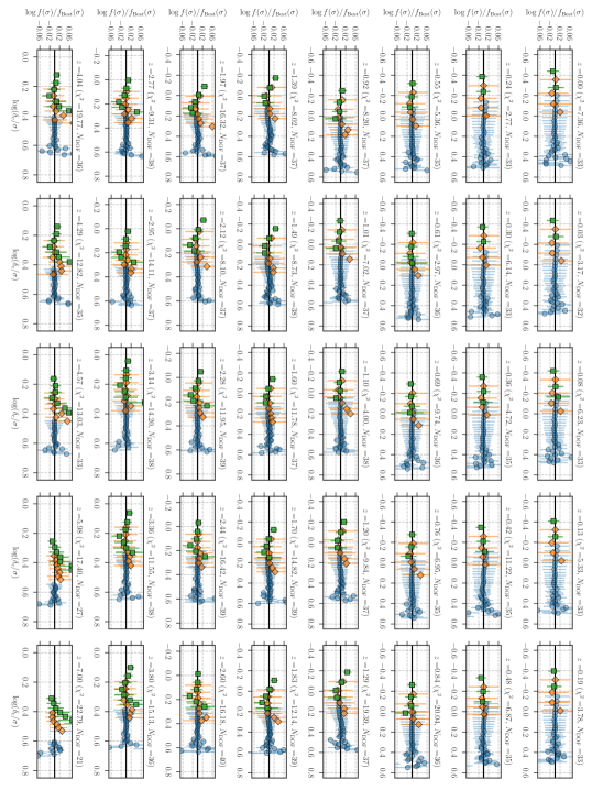
Figure 10: A summary of our fits to virial halo mass functions in the $\nu^{2}$GC simulations. Each panel shows the residual of the multiplicity function $f$ in logarithmic space at different redshifts ($0\leq z\leq 7$). The colored symbols in each panel represent the residual between the simulation result and its best-fitted model and the black line shows no difference between the two. The blue circles, orange diamonds, and green squares are the results in the L, H2, and phi1 runs, respectively.

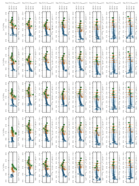
Figure 11: Similar to Figure 10, but we show the residual between the simulation results and the model with Eq. (17)-(20).

References

- Adhikari et al. (2017) Adhikari, R., Agostini, M., Ky, N. A., et al. 2017, J. Cosmology Astropart. Phys, 2017, 025, doi: 10.1088/1475-7516/2017/01/025
- Allen et al. (2011) Allen, S. W., Evrard, A. E., & Mantz, A. B. 2011, ARA&A, 49, 409, doi: 10.1146/annurev-astro-081710-102514
- Baur et al. (2016) Baur, J., Palanque-Delabrouille, N., Yèche, C., Magneville, C., & Viel, M. 2016, J. Cosmology Astropart. Phys, 2016, 012, doi: 10.1088/1475-7516/2016/08/012
- Behroozi et al. (2013) Behroozi, P. S., Wechsler, R. H., & Wu, H.-Y. 2013, ApJ, 762, 109, doi: 10.1088/0004-637X/762/2/109
- Beltz-Mohrmann & Berlind (2021) Beltz-Mohrmann, G. D., & Berlind, A. A. 2021, arXiv e-prints, arXiv:2103.05076. https://arxiv.org/abs/2103.05076
- Benitez-Llambay & Frenk (2020) Benitez-Llambay, A., & Frenk, C. 2020, MNRAS, 498, 4887, doi: 10.1093/mnras/staa2698
- Benítez-Llambay et al. (2017) Benítez-Llambay, A., Navarro, J. F., Frenk, C. S., et al. 2017, MNRAS, 465, 3913, doi: 10.1093/mnras/stw2982
- Berezinsky et al. (2003) Berezinsky, V., Dokuchaev, V., & Eroshenko, Y. 2003, Phys. Rev. D, 68, 103003, doi: 10.1103/PhysRevD.68.103003
- Bertschinger (2006) Bertschinger, E. 2006, Phys. Rev. D, 74, 063509, doi: 10.1103/PhysRevD.74.063509