Free energies of triply and quadruply degenerate electron ladder spectra

Abstract

The electronic free energies in metal clusters are calculated based on a simple ladder spectrum for the level degeneracies three and four, and compared with the known results for degeneracies one and two. The low temperature and the asymptotic high temperature results for free energy differences are generalized to ladder spectra of any degeneracy. Remarkably, free energy differences do not approach zero at high energies for size-independent Fermi energies.

I Introduction

Thermal excitation of electrons is an important contribution to the thermal properties of matter, both in bulk and for metallic clusters and nanoparticles, in spite of the usually relatively small amount of energy contained in these excitations. The finite size of clusters often cause spectra of quasi-free valence electrons in small particles to have gaps that can exceed temperatures by a significant factor. Nevertheless, these excitations will still play an important part in the suppression of size dependent phenomena, such as electronic shell structure [1] or the odd-even effect [2]. Another, related but so far unexplored effect is the thermal suppression of the quantized conductance in one-dimensional conductors, where the quantization of the transverse motion induces both shells and supershells [3] and odd-even effects [4] in analogy to metal clusters [5, 6, 7]. Another effect for which thermally excited electronic states is a sine qua non and which has been explored in some detail is the emission of light from thermally excited photo-active electronic states of gas phase molecules [8, 9, 10, 11, 12, 13, 14]. Other effects have been treated in the early works of [15, 16].

The treatment of the thermal behavior of electrons in most of these situations describing free particles can be considered canonical even if the entire particle is not in equilibrium with an external heat bath that defines a macroscopic temperature. This description is a consequence of the small electronic heat capacity compared to that of the vibrational motion. This makes the vibrational degrees of freedom effectively act as a heat bath, even though the entire system is rigorously microcanonical, as already noted in Ref. [17]. The considerations require that electronic and vibrational energies can be exchanged on timescales shorter than the experimental relevant ones, which will be assumed here. Although there has been observations at low temperatures of cases where this requirement is not fulfilled, it is expected to be the case more often than not, and we will therefore consider the canonical partition functions and corresponding free energies in this work.

One of the original motivations for approaching the question of electronic free energies with the level scheme used here was the question of the temperature dependence of the odd-even effect in simple metal cluster. The question was raised in connection with the abundance pattern in sodium clusters, and was later addressed for gold clusters, which display very strong odd-even effects in several quantities. The original expectation for the sodium clusters was that the effect would disappear asymptotically with temperature, when calculated in the framework of a doubly degenerate (equidistant spacing) ladder spectrum. This, however, was shown in [18] not to be the case. In fact, half the zero temperature Fermi energy difference between odd and even clusters was retained in the free energy in the high temperature limit. It is therefore of obvious interest to know what the analogous values are for larger degeneracies.

Here we will use the equidistant and independent particle spectrum, equivalent to a harmonic oscillator (or ladder) spectrum. The description in terms of independent particles may seem crude, but it is worth to consider how many situations this starting point is made in a statistical treatment, at least as an initial approximation. It is obviously required due to the huge number of states one would otherwise need to calculate to account for any appreciable entropy. The equidistant level spectrum is clearly a schematic representation of real particles. However, the Fermi gas description that works so well on a number of bulk metallic elements, the alkalis in particular, builds successfully on this description. A description of the shell structure of clusters of these metals also reproduces observed shell structure, from the smallest up to up to very large sizes. It has likewise been found to represent gold cluster odd-even staggering caused by the spin degrees of freedom to a surprisingly good accuracy, as judged from the size-dependence of measured dissociation energies in these clusters [18]. We will therefore apply this scheme without any modifications. Finally, in order for the level scheme to mimic the behavior of a Fermi gas in a particle, levels are lowered systematically as sizes increase in order to keep the Fermi energy constant.

One aspect of the level structure calculated should be mentioned, viz. the splitting of levels due to Jahn-Teller deformations. These are not here. To do so would make the theory system specific, yet without being entirely realistic, and it would tend to hide the features the calculations are trying to shed light on, which are the asymptotically high temperature free energy differences mentioned above for the degeneracy two, $g=2$, case. The role of deformations will be considered in the discussion section.

II Computational procedure

The calculation of canonical partition functions for any highly degenerate fermionic systems is complicated due to the combined effect of particle number conservation and Pauli blocking. Several methods have been devised to perform these and related calculations [19, 17, 20]. One method is completely numerical and is based on a two dimensional recurrence where the recurrence variables are the electron numbers and single particle state energies. The equation reads [17]

$$Z(n_{l},N)=Z(n_{l}-1,N)+e^{-\beta\epsilon_{n_{l}}}Z(n_{l}-1,N-1),$$ (1)

where $n_{l}$ numbers the state, and the energy is energy $\epsilon_{n_{l}}$ (we use units where $k_{\rm B}$ is equal to one). A similar equation was suggested for calculating nuclear level densities in [19]. The method in Eq.(1) will be used here as a check of the analytical results obtained.

Another method, specific to the equidistant spectra here, proceeds by convoluting $g$ partition functions for a ladder of degeneracy one to get the total degeneracy $g$ spectrum. The calculation requires an expression for the partition function for the singly degenerate ladder spectrum. The ladder spectrum has energies of the single particle states of

$$E_{n}=\Delta n.$$ (2)

This is known, and is easily calculated with a recurrence relation based on the separation of the sum over configurations into those that have the lowest single particle state occupied and those where it is unoccupied, see e.g. [21]. The result for $N$ electrons is

$$Z_{1}=\prod_{k=1}^{N}\left(1-{\rm e}^{-\beta k\Delta}\right)^{-1},$$ (3)

where the total ground state energy has been set to zero. The free energy of this is shown in Fig. 1.

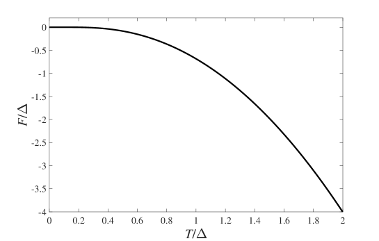
Figure 1: The free energy of the singly degenerate ($g=1$) ladder.

For the degeneracy $g=2$ cases there are two different situations to consider, corresponding to an odd and an even electron number. Both are calculated in the limit of $N\rightarrow\infty$ by adding all possible ground state configurations weighted by the proper Boltzmann factor, and multiplied by $Z_{1}^{2}$. The results are [18], with both ground state energies set to zero,

$$Z_{2}^{\rm e} = Z_{1}^{2}\sum_{m=-\infty}^{\infty}{\rm e}^{-\beta\Delta m^{2}}$$ (4)

$$Z_{2}^{\rm o} = Z_{1}^{2}\sum_{m=-\infty}^{\infty}{\rm e}^{-\beta\Delta m(m-1)}.$$ (5)

However, adding one electron (arriving with a monovalent atom) to a particle will lower the levels. We assume here and for the other cases that this lowering occurs linearly with the number of electrons added. Keeping the energy of the highest occupied orbitals of systems $N$ and $N+2$ identical determines the shift in energy and the additional, relative Boltzmann factor between the even and the odd electron number particle. We have:

$$Z_{2}^{\rm e} = Z_{1}^{2}\sum_{m=-\infty}^{\infty}{\rm e}^{-\beta\Delta m^{2}}$$ (6)

$$Z_{2}^{\rm o} = Z_{1}^{2}{\rm e}^{-\beta\Delta/2}\sum_{m=-\infty}^{\infty}{\rm e}^{-\beta\Delta m(m-1)}.$$ (7)

The corresponding free energies are shown in Fig. 2, and Fig. 3 shows the difference of the free energies.

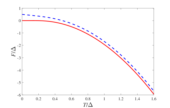
Figure 2: The free energies of the doubly degenerate ladder for odd (dashed line) and even (full line) electron numbers.

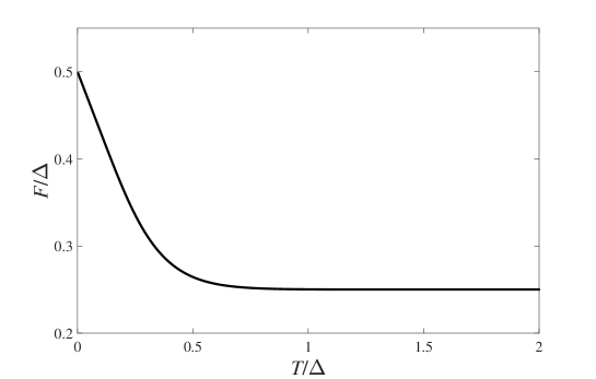
Figure 3: The difference in free energies ($F_{2}^{\rm o}-F_{2}^{\rm e}$) between the odd and the even electron number degenerate ladders.

One particularly interesting result is the fact that the free energy difference does not approach zero for high temperatures, but converges to $\Delta/4$, i.e. half the zero temperature difference. Another interesting result is that this asymptotic value is approached at temperatures significantly below $\Delta$.

For a general value of the degeneracy the expression for the partition function is

$$Z=Z_{1}^{g}\sum_{(n_{1},n_{2},...n_{g})}{\rm e}^{-\beta E^{(0)}(n_{1},n_{2},...,n_{g})},$$ (8)

where $n_{i}$ is now the number of electrons in ladder number $i$. The summation ranges over all possible values of the set of $n$’s, i.e. non-negative values that obey the constraint

$$\sum_{i}n_{i}=N.$$ (9)

The total ground state energy for any specific distribution of electrons on the $g$ different ladders is then, with the zero of energy chosen as the common ground state energy for the single particle states, equal to

$$E^{(0)}(n_{1},n_{2},...,n_{g})=\Delta\sum_{i=1}^{g}\frac{1}{2}n_{i}(n_{i}-1).$$ (10)

For $g=3$ this is

$$E^{(0)}(n_{1},n_{2},n_{3})=\frac{\Delta}{2}\left[n_{1}(n_{1}-1)+n_{2}(n_{2}-1)+n_{3}(n_{3}-1)\right].$$ (11)

The fixed particle number is implemented by eliminating $n_{3}$ with the relation

$$N=n_{1}+n_{2}+n_{3},$$ (12)

to get

$$E^{(0)}(n_{1},n_{2})=\frac{\Delta}{2}\left[2n_{1}^{2}+2n_{2}^{2}+N^{2}-N+2n_{1}n_{2}-2N(n_{1}+n_{2})\right].$$ (13)

In this expression $n_{1}$ and $n_{2}$ can take any non-negative values as long as their sum does not exceed $N$,

$$n_{1}+n_{2}\leq N.$$ (14)

The energy has minimum around $n_{1},n_{2}=(N/3,N/3)$, possibly with a small degeneracy, and hence we also have the minimum for $n_{3}$ around $N/3$.

The value of $N$ is arbitrary, in the sense that as long as it is large enough it will not matter precisely how large. It therefore makes sense to eliminate this number. This is done by redefining the occupation numbers by subtraction of the values pertaining to the absolute ground state. We consider the values $N=3M+f$, with $M$ a large integer, where $f$ takes the values 0, 1 or 2, corresponding to a filled shell, or 1 or 2 additional electrons. Irrespective of the value of $f$ we subtract $M$ from all $n_{i}$. This gives

$$E^{(0)}(n_{1},n_{2})=\frac{\Delta}{2}\left[2n_{1}^{2}+2n_{2}^{2}+2n_{1}n_{2}-2f(n_{1}+n_{2})-f+f^{2}+3M(M-1)+2Mf\right].$$ (15)

From this we subtract the lowest energy which is attained at $n_{1}=n_{2}=0$ for $f=0$, for $f=1$ at the three sets $(n_{1},n_{2})=(0,0),(1,0),(0,1)$, and for $f=2$ at the three values $(n_{1},n_{2})=(1,0),(0,1),(1,1)$. These energies are zero if the term involving $M$ are subtracted, which we will then do. We then have with the redefined occupation numbers and zeroes of energy the expression

$$E^{(0)}(n_{1},n_{2})=\frac{\Delta}{2}\left[2n_{1}^{2}+2n_{2}^{2}+2n_{1}n_{2}-2f(n_{1}+n_{2})-f+f^{2}\right].$$ (16)

To continue, we complete the squares in this expression. Chose $n_{1}$ as the first. After completing the square also for $n_{2}$, we have

$$E^{(0)}(n_{1},n_{2})=\Delta\left(\left(n_{1}+\frac{1}{2}\left(n_{2}-f\right)\right)^{2}+\frac{3}{4}\left(n_{2}-\frac{1}{3}f\right)^{2}+\frac{f^{2}}{6}-\frac{f}{2}\right).$$ (17)

As a check we see that the lowest energies are 0 for all three values of $f$. As mentioned above, the ground state energy should change with $f$. The variation corresponds to an additional contribution of $\Delta(f-f^{2}/3)$. Fig. 4 shows the systematically lowered levels for the triply degenerated ladders.

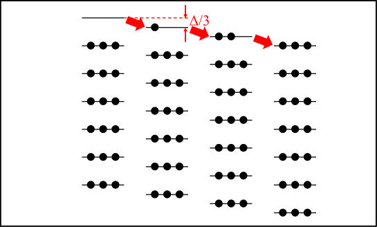
Figure 4: The systemats of the lowering of levels for the triply degenerated ladders. Dots indicate the population of one of the ground states. All lines can accommodate three electrons.

The resulting energy is then

$$E^{(0)}(n_{1},n_{2})=\Delta\left(\left(n_{1}+\frac{1}{2}\left(n_{2}-f\right)\right)^{2}+\frac{3}{4}\left(n_{2}-\frac{1}{3}f\right)^{2}+\frac{1}{2}f-\frac{1}{6}f^{2}\right).$$ (18)

We can now write down the partition function in terms of summations over $n_{1}$ and $n_{2}$:

$$Z_{3}=Z_{1}^{3}{\rm e}^{-\beta\Delta\left(f/2-f^{2}/6\right)}\sum_{n_{1},n_{2}=-\infty}^{\infty}\exp\left(-\beta\Delta\left[\left(n_{1}+\frac{1}{2}\left(n_{2}-f\right)\right)^{2}+\frac{3}{4}\left(n_{2}-\frac{1}{3}f\right)^{2}\right]\right)$$ (19)

The calculation of the sums in this expression depends on the value of $f$, and the summation over $n_{1}$ also depends on $n_{2}$. This gives two contributing sum for each value of $f$. One by one they are:

$f=0,n_{2}$ odd ($n_{2}=2n_{2}^{\prime}+1$):
The term $(n_{2}-f)/2$ in the first bracket is then an integer plus 1/2. As we sum over all integer values of $n_{1}$, the integer part of this term can be set to zero. Eliminating the apostrophe in the following, the contribution from this sector to the sum is then

$$\sum_{n_{1},n_{2}=-\infty}^{\infty}\exp\left(-\beta\Delta\left[\left(n_{1}+n_{2}+\frac{1}{2}\right)^{2}+3\left(n_{2}+\frac{1}{2}\right)^{2}\right]\right),$$ (20)

where $n_{2}$ runs over all integers here and in the following. Thus:

$$\sum_{n_{1}=-\infty}^{\infty}\exp\left[-\beta\Delta\left(n_{1}+\frac{1}{2}\right)^{2}\right]\sum_{n_{2}=-\infty}^{\infty}\exp\left[-3\beta\Delta\left(n_{2}+\frac{1}{2}\right)^{2}\right],$$ (21)

The contribution from $f=0,n_{2}$ even is calculated similarly to give

$$\sum_{n_{1}=-\infty}^{\infty}\exp\left(-\beta\Delta n_{1}^{2}\right)\sum_{n_{2}=-\infty}^{\infty}\exp\left(-3\beta\Delta n_{2}^{2}\right),$$ (22)

To simplify the notation we will define a shorthand for the sums as

$$\sigma(a,b)\equiv\sum_{n=-\infty}^{\infty}\exp\left(-a\beta\Delta(n+b)^{2}\right),$$ (23)

where the dependence on $\beta\Delta$ is implicit. This gives

$$Z_{3}(f=0) = Z_{1}^{3}\left[\sigma(1,0)\sigma(3,0)+\sigma\left(1,\frac{1}{2}\right)\sigma\left(3,\frac{1}{2}\right)\right].$$ (24)

For $f=1$ we have

$$Z_{3}(f=1) = {\rm e}^{-\beta\Delta/3}Z_{1}^{3}\left[\sigma(1,0)\sigma\left(3,\frac{1}{3}\right)+\sigma\left(1,\frac{1}{2}\right)\sigma\left(3,-\frac{1}{6}\right)\right],$$ (25)

and for $f=2$ the sums become

$$Z_{3}(f=2) = {\rm e}^{-\beta\Delta/3}Z_{1}^{3}\left[\sigma\left(1,\frac{1}{2}\right)\sigma\left(3,\frac{1}{6}\right)+\sigma\left(1,0\right)\sigma\left(3,-\frac{1}{3}\right)\right].$$ (26)

Fig. 5 shows the free energies calculated with these equations, performing the summation numerically. Fig. 6 shows the difference of the free energies of the partially occupied systems relative to the closed shell, $f=0$, system.

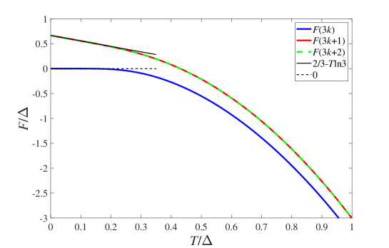
Figure 5: The free energies of the triply degenerate ladder. The lowest (blue) curve gives the $f=0$ case, and the upper are the two numerical identical curves for $f=1$ and $f=2$. The short straight lines are the first order temperature approximations.

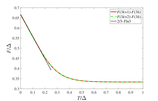
Figure 6: The free energy difference between the $f=1,2$ ladders and the closed shell, $f=0$, ladder systems. The straight line is the first order temperature approximation of the difference.

Figs. 5,6 also show the free energy and free energy difference calculated to first order in the temperature. The approximations, $F=E(0)-TS(0)$, are calculated with the entropies calculated from the ground state degeneracies which are given by the combinatorial factors $C_{3}^{k},k=0,1,2$:

$$S(T=0,f=0) = \ln(C_{3}^{0})=0$$ (27)

$$S(T=0,f=1) = \ln(C_{3}^{1})=\ln 3$$ (28)

$$S(T=0,f=2) = \ln(C_{3}^{2})=\ln 3.$$ (29)

For $g=4$ the ground state energies calculated analogously take the form

$$E\left(n_{1},n_{2},n_{3}\right) = \frac{\Delta}{2}\{2\left(n_{1}^{2}+n_{2}^{2}+n_{3}^{2}\right)+2\left(n_{1}n_{2}+n_{2}n_{3}+n_{3}n_{1}\right)$$

$$- 2f\left(n_{1}+n_{2}+n_{3}\right)+4M\left(M-1\right)+2Mf+f\left(f-1\right)\},$$

with the total number of electrons equal to $4M+f$. Adding $f(f-1)/2$ to this makes the energy zero for all values of $f$:

$$E\left(n_{1},n_{2},n_{3}\right)=E^{(0)} + \frac{f\left(f-1\right)}{2}\Delta$$ (31)

$$=E^{(0)} + \Delta\biggl{[}\left(n_{1}+\frac{n_{2}}{2}+\frac{n_{3}}{2}-\frac{f}{2}\right)^{2}+\frac{3}{4}\left(n_{2}+\frac{n_{3}}{2}-\frac{f}{3}\right)^{2}$$

$$+ \frac{2}{3}\left(n_{3}-\frac{f}{4}\right)^{2}+\frac{f^{2}}{8}-\frac{f}{2}\biggr{]}.$$

Similar to the procedure used for the $g=3$ case, the ground state energy varies with $f$. This gives an additional contribution of $f-f^{2}/4$ which, notably, is also minus twice the term already present in $f$, similar to the $g=3$ case. Fig.7 shows the systematically lowered levels for the quadruply degenerated ladders.

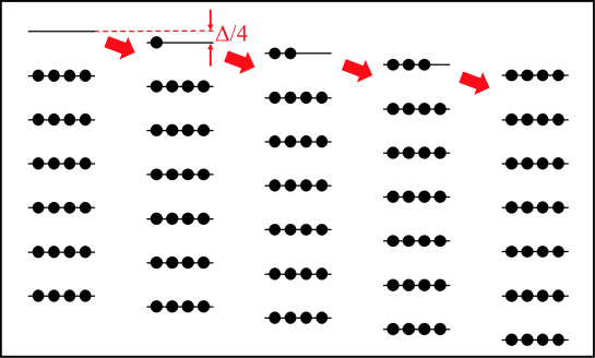
Figure 7: The lowering of levels for the quadruply degenerated ladders, similar to the the $g=3$ case with the difference that lines can accommodate four electrons here.

The resulting energy is then:

$$E\left(n_{1},n_{2},n_{3}\right) = \Delta\biggl{[}\left(n_{1}+\frac{n_{2}}{2}+\frac{n_{3}}{2}-\frac{f}{2}\right)^{2}+\frac{3}{4}\left(n_{2}+\frac{n_{3}}{2}-\frac{f}{3}\right)^{2}$$

$$+ \frac{2}{3}\left(n_{3}-\frac{f}{4}\right)^{2}-\frac{f^{2}}{8}+\frac{f}{2}\biggr{]}.$$

We can now write down the partition function in terms of summations over $n_{1}$, $n_{2}$ and $n_{3}$:

$$Z_{4}=Z_{1}^{4}e^{-\beta\Delta(f/2-f^{2}/8)}\sum_{n_{1},n_{2},n_{3}=-\infty}^{\infty}\exp\biggl{\{}-\beta\Delta\biggl{[}\left(n_{1}+\frac{1}{2}n_{2}+\frac{1}{2}n_{3}-\frac{1}{2}f\right)^{2}$$ (33)

$$+\frac{3}{4}\left(n_{2}+\frac{1}{3}n_{3}-\frac{1}{3}f\right)^{2}+\frac{2}{3}\left(n_{3}-\frac{1}{4}\right)^{2}\biggr{]}\biggr{\}}$$

For each value of $f$ this gives rise to 12 terms. The terms for $f=1,2,3$ are listed in the SI. The sums for $f=0$ are, with $n_{1}$ and the primed summation variables running over all integer values:

$$n_{2}=2n_{2}^{\prime}+1,n_{3}=6n_{3}^{\prime}-2~{}~{}~{}~{}~{}~{} \sigma(1,\frac{1}{2})\sigma(3,\frac{1}{6})\sigma(24,-\frac{1}{3})$$ (34)

$$n_{2}=2n_{2}^{\prime}+1,n_{3}=6n_{3}^{\prime}-1~{}~{}~{}~{}~{}~{} \sigma(1,0)\sigma(3,\frac{1}{3})\sigma(24,-\frac{1}{6})$$ (35)

$$n_{2}=2n_{2}^{\prime}+1,n_{3}=6n_{3}^{\prime}~{}~{}~{}~{}~{}~{} \sigma(1,\frac{1}{2})\sigma(3,\frac{1}{2})\sigma(24,0)$$ (36)

$$n_{2}=2n_{2}^{\prime}+1,n_{3}=6n_{3}^{\prime}+1~{}~{}~{}~{}~{}~{} \sigma(1,0)\sigma(3,\frac{2}{3})\sigma(24,\frac{1}{6})$$ (37)

$$n_{2}=2n_{2}^{\prime}+1,n_{3}=6n_{3}^{\prime}+2~{}~{}~{}~{}~{}~{} \sigma(1,\frac{1}{2})\sigma(3,\frac{5}{6})\sigma(24,\frac{1}{3})$$ (38)

$$n_{2}=2n_{2}^{\prime}+1,n_{3}=6n_{3}^{\prime}+3~{}~{}~{}~{}~{}~{} \sigma(1,0)\sigma(3,0)\sigma(24,\frac{1}{2})$$ (39)

$$n_{2}=2n_{2}^{\prime},n_{3}=6n_{3}^{\prime}-2~{}~{}~{}~{}~{}~{} \sigma(1,0)\sigma(3,-\frac{1}{3})\sigma(24,-\frac{1}{3})$$ (40)

$$n_{2}=2n_{2}^{\prime},n_{3}=6n_{3}^{\prime}-1~{}~{}~{}~{}~{}~{} \sigma(1,\frac{1}{2})\sigma(3,-\frac{1}{6})\sigma(24,-\frac{1}{6})$$ (41)

$$n_{2}=2n_{2}^{\prime},n_{3}=6n_{3}^{\prime}~{}~{}~{}~{}~{}~{} \sigma(1,0)\sigma(3,0)\sigma(24,0)$$ (42)

$$n_{2}=2n_{2}^{\prime},n_{3}=6n_{3}^{\prime}+1~{}~{}~{}~{}~{}~{} \sigma(1,\frac{1}{2})\sigma(3,\frac{1}{6})\sigma(24,\frac{1}{6})$$ (43)

$$n_{2}=2n_{2}^{\prime},n_{3}=6n_{3}^{\prime}+2~{}~{}~{}~{}~{}~{} \sigma(1,0)\sigma(3,\frac{1}{3})\sigma(24,\frac{1}{3})$$ (44)

$$n_{2}=2n_{2}^{\prime},n_{3}=6n_{3}^{\prime}+3~{}~{}~{}~{}~{}~{} \sigma(1,\frac{1}{2})\sigma(3,\frac{1}{2})\sigma(24,\frac{1}{2})$$ (45)

These, and the analogous expressions for the three other $f$ values, can be condensed somewhat by noticing some relations between the $\sigma$ functions:

$$\sigma(a,b)=\sigma(a,-b)=\sigma(a,1-b)$$ (46)

$$\sigma(a,b)+\sigma(a,b+1/2)=\sigma(a/4,2b).$$ (47)

The total partition functions for the four cases then are:

$$Z_{4}(f=0) = Z_{1}^{4}(2\sigma(1,1/2)\sigma(3,1/6)\sigma(6,1/3)$$

$$+ \sigma(1,1/2)\sigma(3,1/2)\sigma(6,0)$$

$$+ 2\sigma(1,0)\sigma(3,1/3)\sigma(6,1/3)$$

$$+ \sigma(1,0)\sigma(3,0)\sigma(6,0)),$$

$$Z_{4}(f=1) = Z_{1}^{4}e^{-\frac{3}{8}\beta\Delta}(\sigma(1,1/2)\sigma(3,1/6)\sigma(3/2,1/6)$$

$$+ \sigma(1,1/2)\sigma(3,1/2)\sigma(6,1/4)$$

$$+ \sigma(1,1/2)\sigma(3,1/3)\sigma(6,5/12)$$

$$+ \sigma(1,0)\sigma(3,0)\sigma(6,1/4)$$

$$+ \sigma(1,0)\sigma(3,1/3)\sigma(6,1/12)),$$

$$Z_{4}(f=2) = Z_{1}^{4}e^{-\frac{1}{2}\beta\Delta}(2\sigma(1,1/2)\sigma(3,1/6)\sigma(6,1/6)$$

$$+ 2\sigma(1,1/2)\sigma(3,1/2)\sigma(24,1/4)$$

$$+ 2\sigma(1,0)\sigma(3,0)\sigma(24,1/4)$$

$$+ 2\sigma(1,0)\sigma(3,1/3)\sigma(6,1/6)$$

$$Z_{4}(f=3) = Z_{1}^{4}e^{-\frac{3}{8}\beta\Delta}(\sigma(1,1/2)\sigma(3,1/6)\sigma(3/2,1/6)$$

$$+ \sigma(1,0)\sigma(3,1/3)\sigma(3/2,1/6)$$

$$+ \sigma(1,0)\sigma(3,0)\sigma(6,1/4)$$

$$+ \sigma(1,1/2)\sigma(3,1/2)\sigma(6,1/4)).$$

These expression can be used with the high temperature expansion of the sums given in Ref. [18]. Here the sums will be performed numerically. Fig. 8 shows the free energies calculated with these equations. Fig. 9 shows the difference of the free energies of the partially occupied systems relative to the closed shell, $f=0$, system. Note that the fact that the free energy differences approach a constant value for all is readily seen from the fact that the sum of the reciprocal square roots of the products of the three $a$’s is the same for all four $f$’s. This follows from the asymptotic values of the $\sigma$’s which are $\sigma(a,b)\rightarrow\sqrt{\pi/a\beta\Delta},T\rightarrow\infty$.

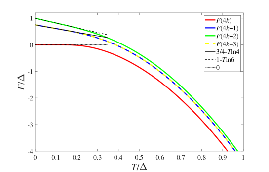
Figure 8: The free energies of the quadruply degenerate ladder. The lowest curve is for the filled shell, $f=0$. The middle curve is for the numerical identical curves for $f=1$ and $f=3$, and the top curve for $f=2$.

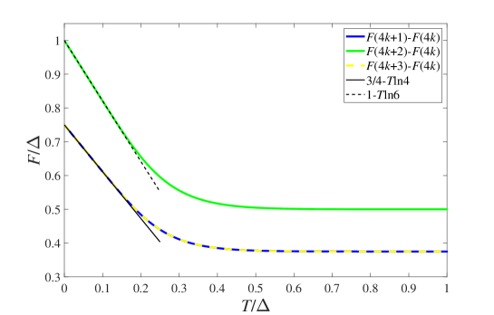
Figure 9: The free energy difference between the $f=1,3$ ladders (lowest curve), $f=2$ (top curve), and the closed shell ladder ($f=0$).

The ground state degeneracies giving rise to the low temperature entropy are calculated as for the $g=3$ case;

$$S(T=0,f=0) = k_{B}\ln(C_{4}^{0})=0$$ (52)

$$S(T=0,f=1) = k_{B}\ln(C_{4}^{1})=\ln 4$$ (53)

$$S(T=0,f=2) = k_{B}\ln(C_{4}^{2})=\ln 6$$ (54)

$$S(T=0,f=3) = k_{B}\ln(C_{4}^{3})=\ln 4.$$ (55)

These can of course equally well be calculated by expanding the sums and collecting the terms with the numerically smallest coefficients of $1/T$ in the exponential.

III Discussion

Two values of the calculated free energies differences between different values of the shell filling parameter $f$ are of special interest, those at zero temperature and at asymptotically high temperatures. The intermediate between these two limits is to a decent approximation represented by a linear interpolation with a slope given by the zero temperature entropy. The zero temperature difference is in all cases twice the difference in the exponential prefactor to the sums. This is also clear from the derivation with the addition of the quadratic form in $f\Delta$, at least for the cases derived here. We expect this will hold also for larger $g$’s, because both the ground state energies and the variation of the added terms that adjust the total energy depend only on $f$ to second order. Basically, a linearly decreasing ladder combined with a linearly increasing occupation number for the highest level will produce a parabolic dependence, irrespective of the value of $g$.

The high temperature limit of the free energy differences is established by approximating the sums in the $\sigma$’s with the corresponding integrals. It is clear from the form of Eq. (II) and the generalization to larger $g$’s that the asymptotically leading order terms will be identical for the sums of all values of $f$, and that this part of the partition function will therefore be asymptotically identical for all $f$. The difference in free energies for different values of $f$ for same ladder spectrum will consequently only depend on the Boltzmann prefactor involving $f$ and $\Delta$. As this contribution to the free energy is temperature independent, we can simply set the value to an $f$ dependent constant plus an $f$-independent contribution:

$$F\rightarrow F_{g,f}+F_{g}(T),~{}~{}~{}~{}T\rightarrow\infty,$$ (56)

where

$$F_{g,f}=\frac{1}{2}\Delta\left(1-f/g\right)f$$ (57)

and

$$F_{g}(T)=-\frac{gT}{2}\ln\left(\frac{\pi T}{\Delta}\right).$$ (58)

The zero temperature approximations are given by

$$F(0)=\Delta\left(1-f/g\right)f.$$ (59)

The zero temperature is given as the logarithm of the relevant binomial coefficient

$$S(0)=\ln(C_{g}^{f}).$$ (60)

At this point it is appropriate to discuss the effects of the level splitting induced by the Jahn-Teller deformations. The effect is fundamentally a matter of energy optimization. With finite temperatures one must instead consider free energy optimization. Even in the best case where ground state deformations had been determined, this makes level splittings temperature dependent and the issue of determining the optimal geometry at finite temperatures one of selfconsistency. Adding material constants as in particular surface tension or bond stiffness will compound the problems.

IV Summary

We have calculated the Helmholtz free energy for a schematic metal particle with degeneracies three and four. The particle has a average Fermi energy, or HOMO level, which is independent of size, consistent with a constant density Fermi gas, and the results refer to this zero of energy. We find that the zero temperature, the low temperature and the high temperature differences in free energies can be described by simple relations determined by the gap parameter and the degeneracy of the levels, in addition to the number of electrons in the upper level. The results generalize to a zero free energy relative to the filled shell ($f=0$) value of $F_{g}(f)-F_{g}(0)=\Delta/g\times(g-f)f$. This values decreases with temperature approximately with the ground state entropy which is given by the binomial coefficient $C_{g}^{f}$ and reaches an asymptotic value of half the $T=0$ difference, $\Delta/2g\times(g-f)f$.

V Author contribution statements

KH conceived the idea and calculated the $g=3$ analytical case. ML and ZS calculated jointly the $g=4$ case analytically and the $g=3$ and $g=4$ cases numerically, and plotted the data. KH wrote the paper.

References

- Genzken and Brack [1991] O. Genzken and M. Brack, Phys. Rev. Lett. 67, 3286 (1991).
- Mottelson [1992] B. R. Mottelson, in Clustering Phenomena in Atoms and Nuclei, edited by M. Brenner, Lönnroth, and F. B. Malik (Springer-Verlag, Berlin, 1992) pp. 571 – 581.
- Yanson et al. [2000] A. Yanson, I. Yanson, and J. van Ruitenbeek, Physical review letters 84, 5832 (2000).
- Yamaguchi et al. [1997] F. Yamaguchi, T. Yamada, and Y. Yamamoto, Solid State Com. 102, 779 (1997).
- Pedersen et al. [1991] J. Pedersen, S. Bjørnholm, J. Borggreen, K. Hansen, T. P. Martin, and H. Rasmussen, Nature 353, 733 (1991).
- Saunders et al. [1985] W. Saunders, K. Clemenger, W. de Heer, and W. Knight, Phys. Rev. B 32, 1366 (1985).
- Manninen et al. [1994] M. Manninen, J. Mansikka-aho, H. Nishioka, and Y. Takahashi, Z. Phys. D 31, 259 (1994).
- Andersen et al. [1996] J. U. Andersen, C. Brink, P. Hvelplund, M. O. Larsson, B. B. Nielsen, and H. Shen, Phys. Rev. Lett. 77, 3991 (1996).
- Andersen et al. [2001] J. Andersen, C. Gottrup, K. Hansen, P. Hvelplund, and M. O. Larsson, Eur. Phys. J. D 17, 189 (2001).
- Toker et al. [2007] Y. Toker, O. Aviv, M. Eritt, M. L. Rappaport, O. Heber, D. Schwalm, and D. Zajfman, Phys. Rev. A 76, 053201 (2007).
- Martin et al. [2013] S. Martin, J. Bernard, R. Brédy, B. Concina, C. Joblin, M. Ji, C. Ortéga, and L. Chen, Phys. Rev. Lett. 110, 063003 (2013).
- Ebara et al. [2016] Y. Ebara, T. Furukawa, J. Matsumoto, H. Tanuma, T. Azuma, H. Shiromaru, and K. Hansen, Phys. Rev. Lett. 117, 133004 (2016).
- Ferrari et al. [2019] P. Ferrari, E. Janssens, P. Lievens, and K. Hansen, Int. Rev. Phys. Chem. 38, 405 (2019).
- Saito et al. [2020] M. Saito, H. Kubota, K. Yamasa, K. Suzuki, T. Majima, and H. Tsuchida, Phys. Rev. A 102, 012820 (2020).
- Kubo [1962] R. Kubo, J. Phys. Soc. Japan 17, 975 (1962).
- Denton et al. [1973] R. Denton, B. Mühlschlegel, and D. J. Scalapino, Phys. Rev. B 7, 3589 (1973).
- Brack et al. [1991] M. Brack, O. Genzken, and K. Hansen, Z. Phys. D 21, 65 (1991).
- Hansen [2020] K. Hansen, Chem. Phys. 530, 110637(1 (2020).
- Frederick C.Williams [1969] J. Frederick C.Williams, Nuclear Physics A 133, 33 (1969).
- Borrmann and Franke [1993] P. Borrmann and G. Franke, J. Chem. Phys. 98, 2484 (1993).
- Schönhammer [2000] K. Schönhammer, Am. J. Phys. 68, 1032 (2000).