Direct Calculation of the Eddy Viscosity Operator in Turbulent Channel Flow at Re_τ=180

Abstract

This study aims to quantify how turbulence in a channel flow mixes momentum in the mean sense. We applied the macroscopic forcing method (Mani and Park, Physical Review Fluids, 2021, p.054607) to direct numerical simulation (DNS) of a turbulent channel flow at Re_τ=180 using two different forcing strategies that are designed to separately assess the anisotropy and nonlocality of momentum mixing. In the first strategy, the leading term of the Kramers-Moyal expansion of the eddy viscosity is quantified, revealing all 81 tensorial coefficients that essentially characterize the local-limit eddy viscosity. The results indicate: (1) the eddy viscosity has significant anisotropy, (2) Reynolds stresses are generated by both the mean strain rate and mean rotation rate tensors associated with the momentum field, and (3) the local-limit eddy viscosity generates asymmetric Reynolds stress tensors. In the second strategy, the eddy viscosity is quantified as an integration kernel revealing the nonlocal influence of the mean momentum gradient at each wall-normal coordinate on all nine components of the Reynolds stresses over the channel width. Our results indicate that while the shear component of the Reynolds stress is reasonably controlled by the local mean gradients, other components of the Reynolds stress are highly nonlocal. These results provide an understanding of anisotropy and nonlocality requirements for closure modeling of momentum transport in wall-bounded turbulent flows.

1 Introduction

Many of the turbulence models in use today are based on the Boussinesq approximation (Boussinesq, 1877) in which the Reynolds stresses are assumed to be a linear function of the local mean velocity gradients. This approximation furthermore assumes isotropy of the tensor representing the coefficients of this linear relation, which is commonly referred to as eddy viscosity. The two simplifications offered by the Boussinesq approximation reduce the job of turbulence modeling to a determination of a scalar eddy viscosity field from which local Reynolds stresses can be determined algebraically without the need to solve any additional equations. For cases in which a single component of the Reynolds stress plays the dominant role, such as in parallel flows, a scalar eddy viscosity can be tuned to yield acceptable Reynolds stress fields (Pope, 2001). However, most turbulence models utilize this approximation even for multi-dimensional flows (Spalart & Allmaras, 1994; Chien, 1982; Menter, 1994; Durbin, 1993; Hanjalić & Launder, 1972; Wilcox, 2008). While some models allow anisotropic eddy viscosities (Spalart, 2000; Mani et al., 2013; Rumsey et al., 2020), they still retain the locality of the Reynolds stress dependence on the mean velocity gradient.

Experimental measurements, as well as DNS data suggest that the isotropy and locality assumptions of the Boussinesq approximation are not strictly valid. Several studies have shown significant misalignment between the principal axis of the Reynolds stress and strain rate tensors indicating non-negligible anisotropy of the eddy viscosity operator (Rogallo, 1981; Rogers & Moin, 1987; Champagne et al., 1970; Harris et al., 1977; Moin & Kim, 1982; Coleman et al., 1996). Furthermore, the assumption of Reynolds stress locality is often not true because turbulent mixing may exist from the history of the straining in a given region of a turbulent flow. For instance, the experiment conducted by Warhaft (1980) showed that the Reynolds stress can arise from the history effects of straining, even with a locally zero mean strain rate. In this case, the Reynolds stress should incorporate temporal or spatial nonlocality of the strain rate tensor.

Given these pieces of evidence, various modeling techniques have attempted to relax both locality and isotropy assumptions via development of second-order closure models (Wilcox et al., 1998; Speziale et al., 1991; Cécora et al., 2015; Launder et al., 1975; Gerolymos et al., 2012) often using the Reynolds stress transport equation as a framework to identify the needed closures. Each of these models, provides a specific way in which Reynolds stresses could depend nonlocally or anisotropically on the velocity gradient field. However, standard data of turbulent flows, either from DNS or experiments, does not provide sufficient information to allow proper discrimination between these models. While these data reveal anisotropy of the Reynolds stresses, they do not uniquely determine the anisotropy or nonlocality of the closure operators that express their dependence on the mean velocity gradient. Closing this gap would require quantification of the eddy viscosity as an operator acting on the mean velocity gradient. With this goal in mind, this study presents a direct quantification of the eddy viscosity operator in a canonical turbulent flow via utilization of the macroscopic forcing method (MFM), developed by Mani & Park (2021).

Prior to the description of our work, we start by reviewing generalized forms of the eddy diffusivity and eddy viscosity operators for scalar and momentum transport in turbulent flows. Firstly, one way of generalizing the Boussinesq approximation is to allow for the anisotropy of the eddy viscosity. Batchelor (1949) suggested using a second-order tensor replacing the diffusion coefficient in the Fickian model to describe the mean transport of a scalar quantity. Later, a similar concept was suggested by Rogers et al. (1989), where the mean turbulent flux of a passive scalar was approximated with an algebraic model expressed in a second-order tensor eddy diffusivity. This anisotropic eddy diffusivity model can be written as the following: $-\overline{u^{\prime}_{i}c^{\prime}}=D_{ij}\partialderivative*{C}{x_{j}}$ where $\overline{(\cdot)}$ represents ensemble-average, $u^{\prime}_{i}$ represents the fluctuation of the velocity, $C$ and $c^{\prime}$ represent the mean and the fluctuation of the scalar quantity being transported, $x_{i}$ represents the coordinate system, and $D^{0}_{ij}$ represents the second-order eddy diffusivity tensor that is local.

Similarly, for the turbulent momentum flux, one method of generalizing the Boussinesq approximation is to use a tensorial representation of the eddy viscosity. Hinze (1959) has suggested the use of the fourth-order tensor as the eddy viscosity. Later, Stanišić & Groves (1965) conducted a systematic investigation of the tensorial character of the eddy viscosity coefficient and revealed that the eddy viscosity tensor has to be at minimum fourth-order. In parallel to the anisotropic eddy diffusivity model, the anisotropic eddy viscosity model for momentum transport can be written as: $-\overline{u^{\prime}_{i}u^{\prime}_{j}}=D^{0}_{ijkl}\partialderivative*{U_{l}}{x_{k}}$ where $U_{l}$ represents mean velocity field. Here, the Reynolds stresses $\overline{u^{\prime}_{i}u^{\prime}_{j}}$ is locally closed in terms of the fourth-order tensorial eddy viscosity $D^{0}_{ijkl}$ and the mean velocity gradient.

An even more general form of the eddy viscosity can be used to incorporate not only anisotropy but also nonlocality. Hamba (2005, 2013) suggested writing the closure of the Reynolds stress in terms of the mean velocity gradient at remote times and locations. This form of eddy viscosity involves a fourth-order tensorial kernel, which we refer to as the eddy viscosity kernel. For statistically stationary flows, this relation can be expressed as

$$-\overline{u_{i}^{\prime}u_{j}^{\prime}}(\mathbf{x})=\int D_{ijkl}(\mathbf{x},\mathbf{y})\left.\partialderivative{U_{l}}{x_{k}}\right|_{\mathbf{y}}\differential[3]{\mathbf{y}},$$ (1)

where $D_{ijkl}(\mathbf{x},\mathbf{y})$ is the eddy viscosity kernel indicating how mean gradients at location $\mathbf{y}$ result in Reynolds stresses at location $\mathbf{x}$. Hamba (2005) reported the first quantification of the eddy viscosity kernel for a turbulent channel flow using a Green’s function formulation approach based on an earlier work by Kraichnan (1987). However, their study focuses on a subset of the tensorial coefficients, i.e., $D_{ij21}$. This choice is motivated since the mean velocity profile in the channel flow is insensitive to other components of the eddy viscosity kernel, given the mean velocity gradient, $\partial U_{l}/\partial x_{k}$ shown in Equation 1, is nonzero only for $(k,l)=(2,1)$. Nevertheless, quantification of other components of eddy viscosity in this canonical setting would provide significant insights about momentum mixing in the broader context of wall-bounded shear flows. Aside from this shortcoming, Hamba (2005) chose to manually enforce the symmetry $D_{ijkl}=D_{jikl}$ by performing arithmetic averaging of the respective components (i.e., $ij$ and $ji$) of the output data from their simulations. This choice was made given the expectation that the Reynolds stress tensor as the output of Equation 1 must always be symmetric, while the raw kernels did not follow this symmetry.

Recently, Mani & Park (2021) presented an alternative interpretation of Equation 1 in the context of the generalized momentum transport (GMT) equation. GMT can be derived by applying the Reynolds Transport Theorem to momentum transport without constraining the momentum field to be identical to the velocity field. In this context, the Reynolds stress, expressed as $\overline{u_{i}^{\prime}v_{j}^{\prime}}$, is interpreted as the mean product of two conceptually different fields, with $u_{i}$ representing the kinematic displacement of volume acting as a transporter of momentum, and $v_{j}$ representing momentum per unit mass, the quantity of interest that results in friction and pressure. Navier-Stokes (NS) is rendered as a special solution to GMT in which the two fields are constrained to be equal. Specifically, when GMT is supplied with the same boundary conditions and forcing conditions as those in NS, the solution to NS is the only attractor solution to GMT, as shown theoretically and numerically by Mani & Park (2021). With this interpretation, Equation (1) is in fact a closure operator to the ensemble-averaged GMT and not the Reynolds Averaged Navier-Stokes (RANS) equation. Therefore, $D_{ijkl}$ and $D_{jikl}$ are not required to be equal, since $\overline{u_{i}^{\prime}v_{j}^{\prime}}\neq\overline{u_{j}^{\prime}v_{i}^{\prime}}$. The present study addresses this issue, by examining the raw eddy viscosity operator without any symmetry averaging. We confirm that while the eddy viscosity kernel of channel flow is not symmetric, it still results in symmetric Reynolds stresses when it acts on the mean velocity gradient of the same flow generating the eddy viscosity.

As previous mentioned, Mani & Park (2021) provides a statistical technique called the macroscopic forcing method (MFM), which allows direct measurement of a flow’s eddy viscosity $D_{ijkl}$ with data gathered from direct numerical simulations (DNS) and GMT. More generally speaking, MFM allows precise computation of RANS closure operators via applying various macroscopic forcing to the GMT equations which can be utilized to extract the eddy viscosity operator. It is worth noting that macroscopic forcing is not limited to delta functions, which reveal Green’s functions as outputs. For instance, Shirian & Mani (2022) employed harmonic forcing to efficiently unveil the eddy diffusivity operator for homogeneous isotropic turbulence. They successfully fitted this operator with an analytical expression. More importantly, Mani & Park (2021) developed inverse macroscopic forcing method (IMFM), in which forcing to constrain mean polynomial fields was shown to reveal nonlocal moments of the underlying eddy diffusivity operator in an economical way compared to the Green’s function approach. This study utilizes this method in our investigation of turbulent channel flow. More specifically, we examine a systematic procedure for obtaining a local operator approximation of the full eddy viscosity operator by considering a Kramers-Moyal expansion (Van Kampen, 1992) of the eddy viscosity operator and quantifying its leading term. This approach does not only enable estimation of the eddy viscosity in an economical fashion, but it also separates out the easy-to-comprehend local eddy viscosity by utilizing this established expansion, which we believe was a missing piece in the analysis of Hamba (2005).

The rest of this paper is organized as follows. In Section 2, we define the flow system and the model used which involves the fourth-order tensorial eddy viscosity kernel, and review the computational methodology. In Section 3, we begin with evaluating the isotropy assumption in the Boussinesq’s approximation. For simplicity, we conduct the leading-order (local-limit) approximation to the eddy viscosity kernel to solely focus on the anisotropy of the eddy viscosity. With the measured local eddy viscosity tensor, we discuss the following: the standard eddy viscosity, the quantified anisotropy, the dependency of Reynolds stress on the rate of rotation, the leading-order Reynolds stress, and the positive definiteness of the leading-order eddy viscosity operator. In Section 4, we extend our study to nonlocal effects, by computing the full eddy viscosity kernel representing the nonlocal effects in the wall-normal direction. In Section 5, we summarize our results and discuss potential extensions to this study.

2 Problem Setup and Governing Equations

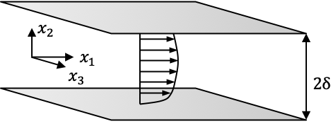
Figure 1: Schematics of the channel flow.

Figure 1 shows the schematics of the channel flow and its coordinate system where the flow is bounded by top and bottom walls spaced $2\delta$ apart. We denote the Cartesian coordinates $x_{i}$, where $x_{1}$ is the streamwise direction, $x_{2}$ is the wall-normal direction, and $x_{3}$ is the spanwise direction. The dimensionless equations expressing mass and momentum conservation are as follows:

$$\partialderivative{u_{i}}{t}+\partialderivative{u_{j}u_{i}}{x_{j}}=-\partialderivative{p}{x_{i}}+\frac{1}{\mathrm{Re}}\partialderivative{u_{i}}{x_{j}}{x_{j}}+r_{i},$$ (2)

$$\partialderivative{u_{j}}{x_{j}}=0,$$ (3)

where $u_{i}$ is the flow velocity, $p$ is the pressure normalized by the density, $t$ is time, and $r_{i}=(1,0,0)$ represents normalized mean pressure gradient. The dimensionless spatial coordinates are normalized by $\delta$, and $\mathrm{Re}$ represents the Reynolds number defined based on $\delta$ and the friction velocity $u_{\tau}=\sqrt{\tau_{w}/\rho}$ where $\tau_{w}$ is the mean wall shear stress balancing the force due to the mean pressure gradient and $\rho$ is the fluid density.

The RANS equations can be obtained by taking the ensemble-average of Equations 2 and 3, yielding:

$$\partialderivative{U_{i}}{t}+\partialderivative{U_{j}U_{i}}{x_{j}}=-\partialderivative{\overline{p}}{x_{i}}+\frac{1}{\mathrm{Re}}\partialderivative{U_{i}}{x_{j}}{x_{j}}-\partialderivative{\overline{u^{\prime}_{j}u^{\prime}_{i}}}{x_{j}}+\overline{r}_{i},$$ (4)

$$\frac{\partial U_{j}}{\partial x_{j}}=0,$$ (5)

where $U_{i}$ is the mean velocity, $u^{\prime}_{i}$ is the velocity fluctuation around the mean velocity, and $\overline{(\cdot)}$ implies ensemble-averaged quantities. To close this system, the divergence of Reynolds stresses, $\partialderivative*{\overline{u^{\prime}_{j}u^{\prime}_{i}}}{x_{j}}$, needs to be modeled in terms of the primary variable $U_{i}$. This can be generally expressed as an operator acting on the ensemble-averaged field, $-\partialderivative*{\overline{u^{\prime}_{j}u^{\prime}_{i}}}{x_{j}}\equiv\overline{\mathcal{L}}\left(U_{i}\right)$. One form of such operators is expressed in Equation (1).

A DNS solution to the channel flow does not provide enough information to fully quantify the nonlocal eddy viscosity kernel, $D_{ijkl}(\mathbf{x},\mathbf{y})$. A full characterization of $D$ requires quantification of Reynolds stresses in response to all possible independent flow gradients scenarios. Following Mani & Park (2021), we next describe the procedure of obtaining $D$. In this paper, however, we limit the scope of our analysis to the one-dimensional RANS context, in which the wall-normal coordinate is the only independent variable since the flow is statistically homogeneous in all other space-time coordinates. In other words, we assume the form: $D_{ijkl}(\mathbf{x},\mathbf{y})=D_{ijkl}(x_{2},y_{2})$, and the other dimensions are integrated out. However, the employed macroscopic forcing methodology is in principle generalizable to multi-dimensional cases, and with higher computational expense can capture the full behavior of $D_{ijkl}(\mathbf{x},\mathbf{y})$.

2.1 Macroscopic Forcing Method

In this section, we discuss details on how to use MFM to measure the eddy viscosity, starting from the generalized momentum transport (GMT) equations.

2.1.1 Generalized Momentum Transport equation

In our earlier work, which was mainly on the transport of passive scalars, we briefly introduced how one can apply MFM to analyze momentum transport (Mani & Park, 2021). To quantitatively determine the eddy viscosity operator, one first needs the detailed velocity field of the specific flow of interest. One method of obtaining such velocity fields is to perform a DNS simulation, which we call the donor simulation, as it donates a velocity field whose eddy viscosity is to be determined.

To analyze momentum transport by a given flow, we will now consider GMT, which can be derived from the Reynolds Transport Theorem for a fluid system with a Fickian model for molecular viscosity.

$$\partialderivative{v_{i}}{t}+\partialderivative{u_{j}v_{i}}{x_{j}}=-\partialderivative{q}{x_{i}}+\frac{1}{\mathrm{Re}}\partialderivative{v_{i}}{x_{j}}{x_{j}}+r_{i},$$ (6)

$$\partialderivative{v_{j}}{x_{j}}=0.$$ (7)

where $v_{i}$ represents momentum per unit mass, and is considered to be different from $u_{i}$ from the donor velocity field. Also, $q$ is the generalized pressure to ensure the incompressibility of the velocity field $v_{i}$.

Equations 6 and 7 then describe a passive solenoidal vector field that is transported by the background velocity field $u_{j}$ governed by Equation 2. An advantage of working with GMT, as opposed to NS, is its linearity with respect to the transported quantity, $v_{i}$. Under such conditions, expressing the generalized eddy viscosity in the format given by Equation 1 becomes meaningful. As discussed by Mani & Park (2021), GMT spans a larger solution space than NS; NS is a special subset of the GMT space where $v_{i}=u_{i}$.

An important question that naturally follows is whether the computed RANS operator of GMT is the same as that of the NS equation. In our earlier work, we already showed analytically and numerically that the macroscopic operators of the GMT and NS equations are identical (Mani & Park, 2021). Moreover, the solutions of GMT and NS equations become microscopically the same after sufficient time regardless of the initial conditions when we apply the same boundary conditions to both equations. The time scale at which the solutions become identical was found to be $\tau_{\textrm{mix}}=16.6\delta/u_{\tau}$ for a turbulent channel flow. Therefore, it is justified that the macroscopic operator of the GMT equation obtained by MFM is the same as the RANS operator of the NS equations. In sum, GMT works as an auxiliary set of equations that probes RANS operator of NS and therefore we can obtain eddy viscosity of the RANS equations by investigating that of the GMT equations.

It is important to note that Hamba (2005) wrote an equation very similar to GMT equations in spite of taking a conceptually different derivation path. His passive vector equation is indeed GMT subtracted by the mean of GMT. The main difference lies in the explicit inclusion of forcing in the equations, allowing for a general macroscopic field. In contrast, Hamba (2005) implicitly applies forcing by specifically considering Dirac delta function mean fields.

2.1.2 Analysis Strategy

We aim to study two aspects of the eddy viscosity kernel in a turbulent channel flow: the anisotropy and the nonlocality. To fully investigate such non-Boussinesq effects, it is ideal to compute every value of the full eddy viscosity kernel $D_{ijkl}$ in Equation 1. Since the channel flow is homogeneous in $x_{1}$ and $x_{3}$ directions and statistically stationary, we integrate the mixing effect in these directions. The simplified Reynolds stress for GMT variables can be expressed as:

$$-\overline{u_{i}^{\prime}v_{j}^{\prime}}(x_{2}) =\int D_{ijkl}({x_{2}},{y_{2}})\left.\frac{\partial V_{l}}{\partial x_{k}}\right|_{{y_{2}}}\mathrm{d}y_{2}.$$ (8)

Equation 8 incorporates anisotropy via tensorial representation and nonlocality via the integration form. MFM has the capability to compute all the elements in the eddy viscosity kernel $D_{ijkl}\left(x_{2},y_{2}\right)$ by tracking the influence of each entry of $dV_{l}/dx_{k}$ on the entire Reynolds stress field. It has been demonstrated by Liu et al. (2021) that such a brute force approach is theoretically equivalent to Hamba’s Green’s function approach (Hamba, 2005).

However, one caveat is that the cost of each simulation is significant and consequently it is not desirable to conduct a full nonlocal MFM analysis. To conduct computation for $D_{ijkl}$ for given $k$ and $l$, one requires as many DNS simulations as the number of degree of freedom of the RANS space. Therefore, to reduce the cost of the analysis, we conduct two separate analyses for the anisotropy and nonlocality, both using MFM.

First, we focus on studying the anisotropic nature of the eddy viscosity. However, to focus exclusively on anisotropy, we systematically construct a local approximation of the eddy viscosity operator using the Kramers-Moyal expansion (Van Kampen, 1992), as investigated by Mani & Park (2021). For instance, in a parallel flow where $dV_{1}/dx_{2}$ is the only active component of the velocity gradient, the Reynolds stress $\overline{u_{2}^{\prime}v_{1}^{\prime}}$ in Equation 8 can be written as the integral of only $D_{2121}$ component of the eddy viscosity. By considering a Taylor series expansion of $dV_{1}/dx_{2}$ around $y_{2}=x_{2}$, one can re-express the eddy viscosity operator in terms of the following expansion:

$$-\overline{u_{2}^{\prime}v_{1}^{\prime}}(x_{2}) =\int D_{2121}({x_{2}},{y_{2}})\left.\partialderivative{V_{1}}{x_{2}}\right|_{y_{2}}\differential{y_{2}}$$ (9)

$$=\int D_{2121}({x_{2}},{y_{2}})\left(\left.\partialderivative{V_{1}}{x_{2}}\right|_{x_{2}}+(y_{2}-x_{2})\left.\partialderivative[2]{V_{1}}{x_{2}}\right|_{x_{2}}+\cdots\right)\differential{y_{2}}$$ (10)

$$=\sum_{n=0}^{\infty}D^{n}_{2121}({x_{2}})\partialderivative{{}^{n+1}V_{1}}{x_{2}^{n+1}}$$ (11)

where $D^{n}_{2121}=\int{D_{2121}(x_{2},y_{2})(y_{2}-x_{2})^{n}/n!\differential y_{2}}$ represents the $n$-th spatial moment of the eddy viscosity kernel.

As discussed by Mani & Park (2021), the leading term in this expansion encapsulates the local limit eddy viscosity while the subsequent terms characterize finite moments associated with the nonlocal effects. The general form of this leading-order approximation for all components of the Reynolds stress and mean velocity gradient is as below:

$$-\overline{u_{i}^{\prime}v_{j}^{\prime}}(x_{2})=D^{0}_{ijkl}(x_{2})\partialderivative{V_{l}}{x_{k}},$$ (12)

where $D^{0}_{ijkl}(x_{2})$ is called the leading-order eddy viscosity tensor:

$$D^{0}_{ijkl}(x_{2})=\int{D_{ijkl}\differential y_{2}}.$$ (13)

Equation 12 would be exact only when $D_{ijkl}(x_{2},y_{2})$ is local, i.e. $D_{ijkl}(x_{2},y_{2})=D^{0}_{ijkl}(x_{2})\delta(x_{2}-y_{2})$ where $\delta(x)$ is a Dirac delta function.

The local eddy viscosity in Equation 12 is no longer a scalar value varying in space; it is a fourth-order tensor with 81 coefficients. The tensor representation was suggested by previous researchers including Batchelor (1949), but the full quantification has not been conducted to the authors’ knowledge. As presented in Appendix B, using only 9 MFM simulations, we computed all 81 coefficients of the eddy viscosity tensor. The resulting tensor elements are provided in Appendix C.

The next investigation focuses on the nonlocality of the eddy viscosity. As conducting MFM to measure the full kernel can be costly for complex turbulent flow systems, we focus on calculating a subset of tensorial kernel components, specifically the kernel components that are multiplied to $\partial V_{1}/\partial x_{2}$ in Equation 8. The computed tensorial kernel components are $D_{ij21}\left(x_{2},y_{2}\right)$ and they are associated with the Reynolds stresses which correspond to the velocity gradient $\partial U_{1}/\partial x_{2}$, the only velocity gradient appearing in the RANS closure for a channel flow. The detailed steps on how to measure eddy viscosity kernel using MFM is discussed in Appendix E.

2.1.3 Application of Macroscopic Forcing Method

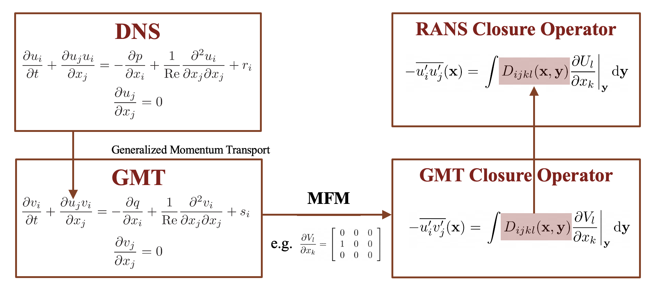
Figure 2: Schematics of the MFM analysis.

The next step involves how we actually compute the leading-order eddy viscosity tensor and the eddy viscosity kernel. Figure 2 illustrates how we conducted our MFM analysis. To apply MFM, we start with two sets of solvers: one for the NS equations and the other for GMT. At each time step, we solve the NS equation to obtain the velocity field $u_{i}$ and feed it as the advecting velocity to the GMT solver. For the GMT equations, we force the Reynolds-averaged GMT variable $V_{i}$ to be a specific value in order to acquire certain information about the eddy viscosity. A forcing field $s_{i}$ that results in $V_{1}=x_{2}$ and $V_{2}=V_{3}=0$ generates GMT data from which we can extract the leading-order eddy viscosity $D^{0}_{ij21}$. More specifically, $D^{0}_{2121}$ can be obtained by post-processing $\overline{u^{\prime}_{2}v^{\prime}_{1}}$ from this GMT simulation, and re-evaluating Equation 9 - 11 to observe:

$$-\overline{u^{\prime}_{2}v^{\prime}_{1}}(x_{2})=\int D_{2121}({x_{2}},{y_{2}})\left.\partialderivative{V_{1}}{x_{2}}\right|_{y_{2}}\differential{y_{2}}\stackrel{{\scriptstyle V_{1}=x_{2}}}{{=}}\int D_{2121}({x_{2}},{y_{2}})\differential{y_{2}}=D^{0}_{2121}(x_{2})$$ (14)

As discussed, the macroscopic operator of the Reynolds-averaged GMT and the RANS operator of NS are identical. Therefore, $D^{0}_{2121}$ corresponds to the standard eddy viscosity $\nu_{T}$ used in the Boussinesq approximation in RANS models. Likewise, we can compute other components of the leading-order eddy viscosity tensor using different selections of the macroscopic forcing field, $s_{i}$, such that other components of the mean velocity gradient are activated.

Additionally, the same setup shown in Figure 2, can be used to compute the full kernel of eddy viscosity. The main difference is to apply macroscopic forcings that would generate mean fields in the form of Dirac delta functions. For example, a macroscopic field, $s_{i}$, that sustains $V_{1}(x_{2})=\delta(x_{2}-y_{2})$, would result in GMT data from which we can extract $D_{ij21}(x_{2},y_{2})$, by merely post processing the $\overline{u^{\prime}_{i}v^{\prime}_{j}}$ data. This specific choice of forcing would result in data similar to those obtained by Hamba (2005), with the difference that Hamba used only the symmetric portion of the momentum flux tensor in order to ensure symmetry of the Reynolds stresses. As we shall see, GMT does not produce symmetric eddy viscosity kernels and thus $D_{ijkl}\neq D_{jikl}$. This is intuitively understandable noting that $D_{ijkl}$ quantifies the rate of mixing of the mean $j$-momentum by the $i$-component of the velocity fluctuations while $D_{jikl}$ quantifies the rate of mixing of the mean $i$-momentum by the $j$-component of the velocity fluctuations. Since in this framework, momentum and velocity fields can be quantitatively different, the symmetry does not hold. Likewise, this asymmetry propagates to the Kramers-Moyal expansion of the eddy viscosity operator, and as we shall see, even the leading-order eddy viscosities are not symmetric.

Lastly, we note that the macroscopic forcing procedure used in this work is an inverse forcing method as discussed by Mani & Park (2021), since we explicitly set the desired mean momentum field $V_{i}$ for each GMT simulation, as opposed to setting the macroscopic forcing field.

2.2 Simulation Setup

We adapt MFM solver to a three-dimensional incompressible NS solver originally developed by Bose et al. (2010) and modified by Seo et al. (2015). The present DNS uses the fractional step method with semi-implicit time advancement (Kim & Moin, 1985). For the temporal difference scheme, we use second order Crank-Nicholson for the wall-normal diffusion and Adams-Bashforth for the rest of the terms. The solver uses a second-order finite spatial discretization on a staggered mesh (Morinishi et al., 1998). Also, we use a uniform grid in the streamwise and spanwise directions and grid-stretching in the wall-normal direction. The domain is periodic both in the spanwise and the streamwise directions, and the no-slip boundary condition is applied at the two walls.

The numerical setup for the GMT solver is almost identical to that of DNS, except for two differences. The first is that GMT obtains the background velocity from the NS solver at every time step. The other difference is that GMT utilizes macroscopic forcing, in order to maintain a desired macroscopic momentum field $V_{i}(x_{2})$. To be most rigorous, the selected macroscopic forcing, $s_{i}(x_{2})$, must be independent of time. Likewise, the resulting mean velocity field needs to match the pre-set $V_{i}(x_{2})$ only after time averaging. However, constraining the simulations in this fashion, would require expensive iterations over which the entire simulation must be repeated after each adjustment of $s_{i}(x_{2})$. To avoid this cost, in our implementation, we computed ensemble averages by averaging fields only in the $x_{1}$ and $x_{3}$ directions, and we constrained $s_{i}(x_{2})$ at each time step such that $V_{i}(x_{2})$ is matched to the pre-set $V_{i}(x_{2})$ at each time step.

However, in this implementation the resulting $s_{i}(x_{2})$ is not perfectly time independent. Due to finite number of samples per time step, fluctuations in time are observed. One remedy to reduce these fluctuations is to increase the number of samples by selecting a longer domain in the $x_{1}$ and $x_{3}$ directions. We have performed such domain convergence studies in Appendix A indicating the adequacy of the selected domain size in our MFM analysis.

There are two sets of forcings for MFM presented in this paper, each corresponding to the analysis of anisotropy and the nonlocality of eddy viscosity (Table 1). Within each set, multiple simulations are performed where the macroscopic forcings are varied to reveal different components of the eddy viscosity. The first set uses GMT simulations under different macroscopic forcings to reveal the leading-order eddy viscosity tensor $D^{0}_{ijkl}$. We utilize these measurements to understand the anisotropy of the eddy viscosity. The second set probes a subset of the entire eddy viscosity kernel, $D_{ij21}$, which quantifies the nonlocality of the eddy viscosity in response to the most significant velocity gradient $\partial U_{1}/\partial x_{2}$. In addition to the analysis method and the resulting eddy viscosity, Table 1 presents the number of total DNSs in each set, the domain size, the spatial resolution, and the sampling times. For the first set, only nine DNSs are needed corresponding to $k,l\in\{1,2,3\}$, and for the second set, MFM analyses require a set of simulations with the number of the macroscopic degree of freedom. The results of each set are discussed in Sections 3 and 4 respectively, and the detailed simulation setup of each set is discussed in Appendix B and C, respectively. Also, the measured eddy viscosities, $D^{0}_{ijkl}$ and $D_{ij21}$, are provided as the supplementary data.

Analysis	Eddy Viscosity	Number of DNS’s	$L_{1}\times L_{2}\times L_{3}$	$N_{1}\times N_{2}\times N_{3}$	$Tu_{\tau}/L_{2}$
Anisotropy	$D^{0}_{ijkl}(x_{2})$	9	$2\pi\times 2\times\pi$	$144\times 144\times 144$	750
Nonlocality	$D_{ij21}(x_{2},y_{2})$	145	$2\pi\times 2\times\pi$	$144\times 144\times 144$	500

Table 1: Simulation setup for anisotropy analysis and nonlocality analysis of the eddy viscosity. $L_{1}\times L_{2}\times L_{3}$ is the domain size, $N_{1}\times N_{2}\times N_{3}$ is the number of grid, and $Tu_{\tau}/L_{2}$ is the total simulation time in wall units.

3 Anisotropy Analysis

In this section, we compute the leading-order eddy viscosity tensor $D^{0}_{ijkl}$ and focus on the analysis on anisotropy of the eddy viscosity and specifically contrast it to the standard eddy viscosity implied by the Boussinesq model. In addition, we assess dependency of Reynolds stresses on the rate of rotation, examine reconstruction of Reynolds stresses using the leading-order eddy viscosity, and lastly discuss positive definiteness of the leading-order eddy viscosity tensor.

3.1 Standard Eddy Viscosity

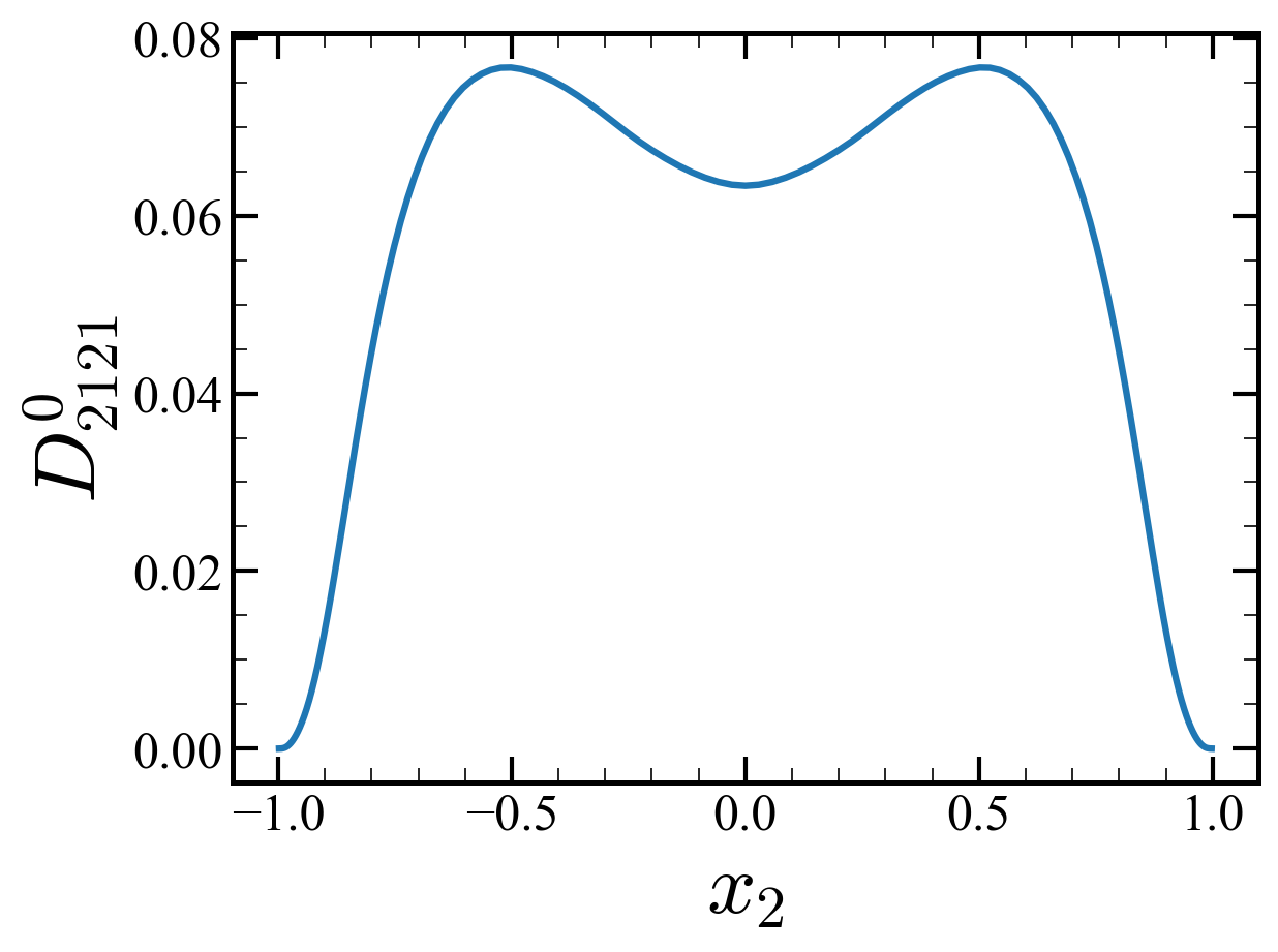
Figure 3: Eddy viscosity element $D^{0}_{2121}$.

In parallel flows, among all the components of the eddy viscosity tensor, by far the most important component is $D^{0}_{2121}$ which represents the mixing effect by $\partialderivative*{U_{1}}{x_{2}}$. This component also corresponds to the standard eddy viscosity $\nu_{T}$. Figure 3 shows the MFM-measured $D^{0}_{2121}$ across the wall-normal dimension $x_{2}$. An important observation here is that the MFM allows us to measure the eddy viscosity at the channel center plane $x_{2}=0$, where the velocity gradient $\partialderivative*{U_{1}}{x_{2}}$ is zero due to the symmetry of the mean velocity profile. This value is unobtainable in typical approaches—tuning $\nu_{T}$ to $\overline{u^{\prime}_{2}u^{\prime}_{1}}/\left(\partialderivative*{U_{1}}{x_{2}}\right)$.

(a) $u^{\prime}_{1}$ contour in $x_{1}$-$x_{3}$ plane

(b) $v^{\prime}_{1}$ contour in $x_{1}$-$x_{3}$ plane

(c) $u^{\prime}_{1}$ contour in $x_{3}$-$x_{2}$ plane

(d) $v^{\prime}_{1}$ contour in $x_{3}$-$x_{2}$ plane

Figure 4: Instantaneous velocity contour of $u^{\prime}_{1}$ and $v^{\prime}_{1}$ in cross-section: (a) and (b) correspond to the cross-section taken at $x_{2}=-0.8492$ and (c) and (d) correspond to the cross-section taken at $x_{1}=3.08$. The shown vector field $v_{i}$ corresponds to a leading-order MFM in which GMT equation is macroscopically forced to achieve $V_{1}=x_{2}$ and $V_{2}=V_{3}=0$.

Figure 4 shows instantaneous field data for the streamwise velocities $u_{1}^{\prime}$ and $v_{1}^{\prime}$ of the MFM simulation for evaluation of $D^{0}_{2121}$ at the same instantaneous time. Figures (a) and (b) show the velocity profile over $(x_{1},x_{3})$ cross-section taken at $x_{2}=-0.8492$ ($x_{2}^{+}=27$) and Figures (c) and (d) show the velocity profile over $(x_{3},x_{2})$ cross-section taken at $x_{1}=3.08$. The key feature shown is that even though the forcings for the NS vector field $u_{i}$ and the GMT vector field $v_{i}$ are completely different macroscopically, MFM leads to similar features in the $u^{\prime}_{1}$ and $v^{\prime}_{1}$. The same qualitative observation holds across all three components of the $u^{\prime}_{i}$ and $v^{\prime}_{i}$ fields. Furthermore, while for $x_{2}<0$ we observe positive correlation between $u^{\prime}_{i}$ and $v^{\prime}_{i}$ fields, the sign of correlation flips for $x_{2}>0$. For this specific MFM analysis, the sole difference between $u^{\prime}_{i}$ and $v^{\prime}_{i}$ fields is in the enforced mean velocity profile. As shown by Mani & Park (2021) without forcing, GMT would result in $v$-fields identical to $u$-fields after a few flow through times regardless of the choice of initial conditions. The case shown in Figure 4 corresponds to a forced GMT in which the mean velocity gradient is kept constant $\partial V_{1}/\partial x_{2}=1$ in order to examine mixing by the leading-order (local limit) eddy viscosity. The observation in Figure 4 suggests that mixing of $u_{1}$ in turbulent channel flow is dominated by the leading-order effects.

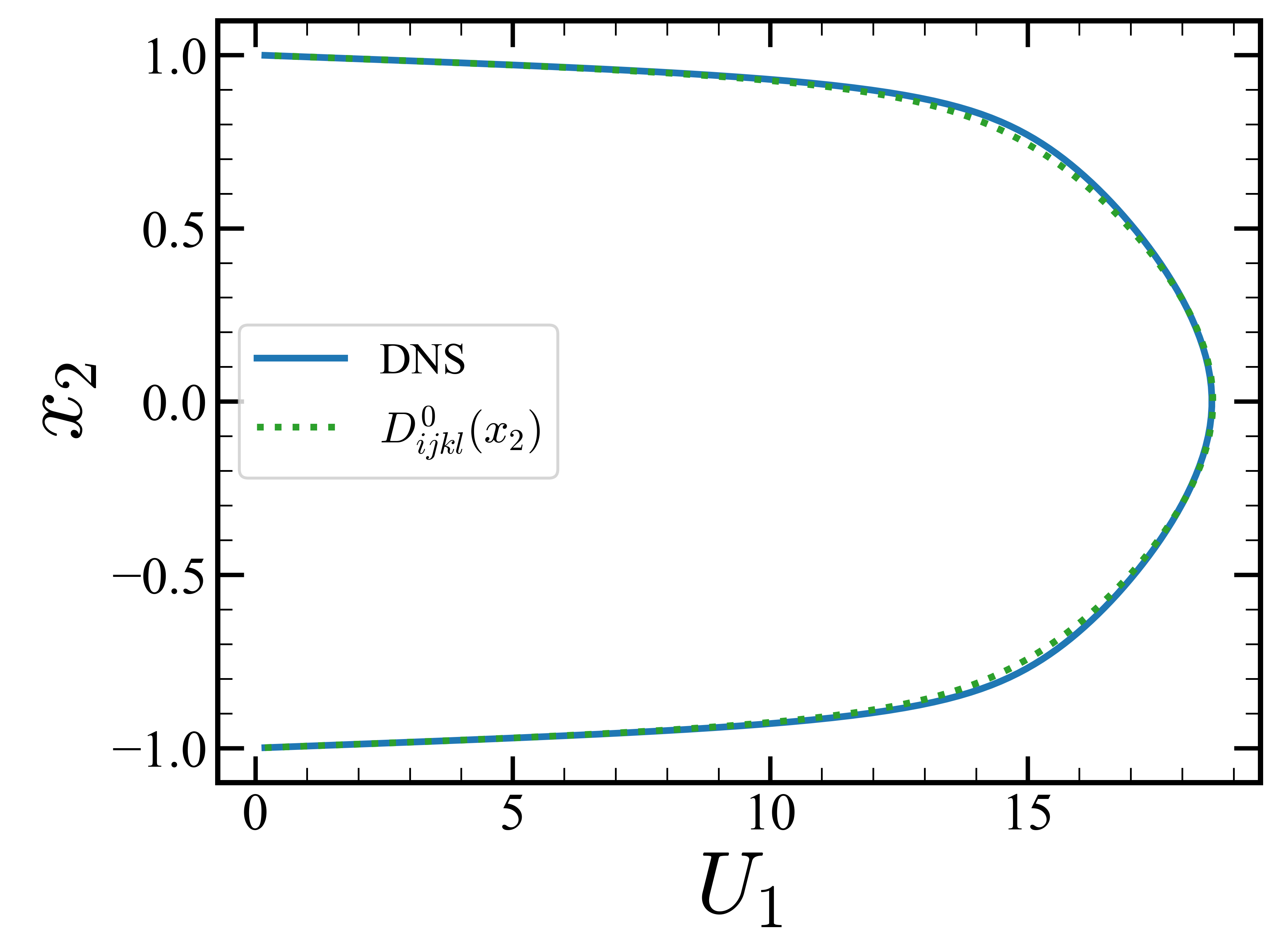
Figure 5: RANS prediction using $D^{0}_{2121}$: dotted green line, mean velocity prediction using $D^{0}_{2121}$ and blue solid line, its comparison to the DNS data.

To assess this conclusion quantitatively we next obtain the RANS solution using the measured $D^{0}_{2121}$ to examine how accurate the leading-order eddy viscosity performs for the prediction of the mean velocity profile. Since the prediction of the mean channel flow only requires one component in the Reynolds stress, we conduct the RANS simulation using $D^{0}_{2121}$ and compare the predicted solution with that of the DNS. As shown in Figure 5, the MFM-based leading-order RANS solution predicts the DNS solution very accurately with an accuracy of 99%. The accuracy is computed with max absolute error $\max\left(U_{1}^{\mathrm{DNS}}-U_{1}^{\mathrm{MFM}}\right)/\max\left(U_{1}^{\mathrm{DNS}}\right)$, where $U_{1}^{\mathrm{DNS}}$ is the streamwise velocity from DNS and $U_{1}^{\mathrm{MFM}}$ is the streamwise velocity predicted from RANS using MFM-measured eddy viscosity $D^{0}_{2121}$. This highly accurate RANS prediction indicates that the nature of the mean momentum mixing in the turbulent channel flow is highly local and the RANS solution of this flow can be predicted using the leading-order approximation.

Other parallel flows like the channel flow have only one active velocity gradient, the wall-normal gradient of streamwise velocity. Additionally, for these flows only one component of the Reynolds stress, the shear component, is mixing momentum. Therefore, as far as prediction of the mean flow is concerned, for these flows anisotropy of the eddy viscosity does not play a role; only $D_{2121}$ needs to be accurate. Furthermore, based on the observed MFM analysis, we conclude that the leading-order eddy viscosity, $D^{0}_{2121}$ provides accurate prediction of momentum mixing, and thus eddy viscosity is local. Therefore, for purely parallel flows, at least for channel flow observed here, both isotropy and locality of the Boussinesq approximation are justified.

Hamba (2005) also reported a small subset of the components of the leading-order (local limit) eddy viscosity, through a more expensive method of first computing the full eddy viscosity kernel for those components and then performing integration as in Equation 13. Our result in Figure 5 regarding locality of momentum mixing is in contrast to his result (see Figure 4 in Hamba (2005)). We attribute this difference to the fact that Hamba used the average of $D^{0}_{2121}$ and $D^{0}_{1221}$ as the representative local eddy viscosity. This averaging was motivated to enforce symmetric Reynolds stresses. However, conceptually these two eddy viscosities represent different mixing rates: the former represents mixing of the streamwise momentum in the wall normal direction, while the latter represents mixing of the wall-normal momentum in the streamwise direction. As we shall see, while a full eddy viscosity kernel reproduces symmetric Reynolds stresses, the leading-order eddy viscosity causes errors not only in magnitude but also in symmetry of Reynolds stresses.

We next use MFM to quantify other components of $D^{0}_{ijkl}$. While these components do not affect prediction of the mean velocity profile in purely parallel flows, they provide an understanding of momentum mixing by this parallel flow, if hypothetical mean momentum gradients were imposed in other directions. Our analysis is motivated by observation of spatially developing turbulent boundary layers, where weak momentum gradient could exist in both streamwise and spanwise directions. These mean gradients induce additional Reynolds stresses, due to components of $D_{ijkl}$ other than $D_{2121}$. Additionally, it has been observed that turbulent boundary layers have similar hairpin structures in their velocity field as those seen in turbulent channel flows (Eitel-Amor et al., 2015), and thus are expected to mix momentum in manners similar to that of a turbulent channel flow. While quantitative differences are expected between the two flows, we expect anisotropy in eddy viscosity observed in turbulent channel flow be at least qualitatively representative of anisotropy encountered in turbulent boundary layers. Given the stringent statistical convergence requirements for MFM simulations, e.g. at least an order of magnitude longer simulations needed than commonly reported DNS, compared to turbulent boundary layers, turbulent channel flows have the advantage of cheaper runtime per time step and availability of additional homogeneous direction for statistical convergence.

3.2 Quantifying Anisotropy

We computed all other components of the anisotropic eddy viscosity tensor $D^{0}_{ijkl}$, a total of 81 coefficients as a function of the wall-normal coordinate. All the data are shown in Appendix C. Out of 81 components, 41 are non-zeros and 40 are inevitably zero due to the symmetry in spanwise direction.

Out of all the elements, the largest eddy viscosity component is $D^{0}_{1111}$, with a maximum value of 1.318, and the smallest nonzero eddy viscosity component is $D^{0}_{2331}$ with the maximum value of 0.00248. After comparing these values to a maximum value of the nominal eddy viscosity $D^{0}_{2121}$, which is 0.0767, we determined that the largest coefficient in the eddy viscosity tensor is one order of magnitude larger than the nominal eddy viscosity and three orders of magnitude larger than the smallest coefficient, indicating a significant anisotropy. When we examine these ratios locally at each $x_{2}$, the differences are more drastic and may go up to a few orders of magnitude. After $D^{0}_{1111}$, the largest eddy viscosity components are $D^{0}_{1212}$ and $D^{0}_{1313}$ with maximum values of 0.573 and 0.407, respectively. All three eddy viscosities have their first and third index represented by the streamwise direction. These indices respectively represent the component of the velocity field that mixes momentum and the direction of the mean-momentum gradient. This observation coincides with the fact that $u^{\prime}_{1}$ is the largest fluctuating velocity component in channel flow. Combining the two observations, we conclude that $u^{\prime}_{1}$ is the strongest mixer of momentum and is most effective in mixing in the $x_{1}$ direction, as intuitively expected. Specifically, mixing rate in the streamwise direction due to streamwise gradients is substantially faster than the standard eddy viscosity which characterises mixing in the wall-normal direction due to wall normal gradients.

Additionally, all three dominant eddy viscosity components have repeated second and fourth indices. These indices respectively represent the momentum component that is being mixed and the momentum component whose mean gradient is responsible for mixing. Based on this observation, we conclude that within $D^{0}_{1j1l}$, mean gradient of component $l$ most effectively contributes to the generation of $\overline{u^{\prime}_{1}v^{\prime}_{j}}$ when $j=l$. In other words, gradient of each momentum component most effectively generates fluxes of the same momentum component at least in the leading-order limit. This latter observation is extendable to $D^{0}_{ijil}$ components.

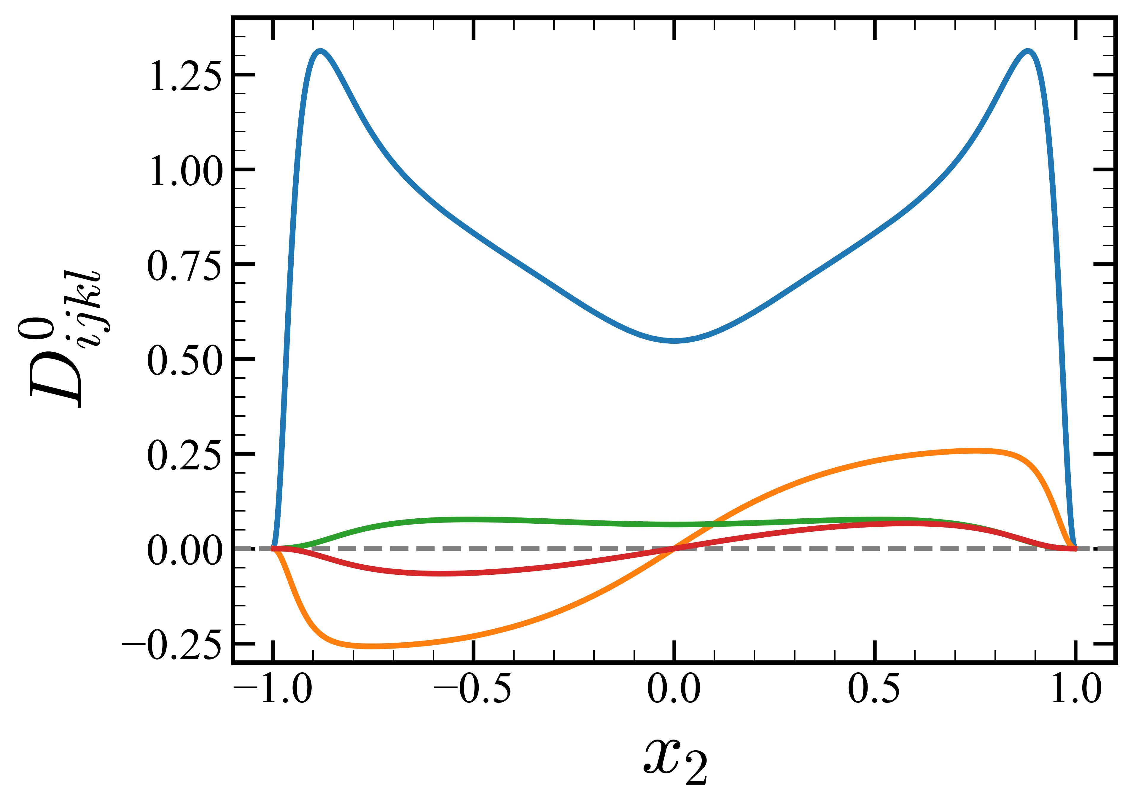
(a) MFM

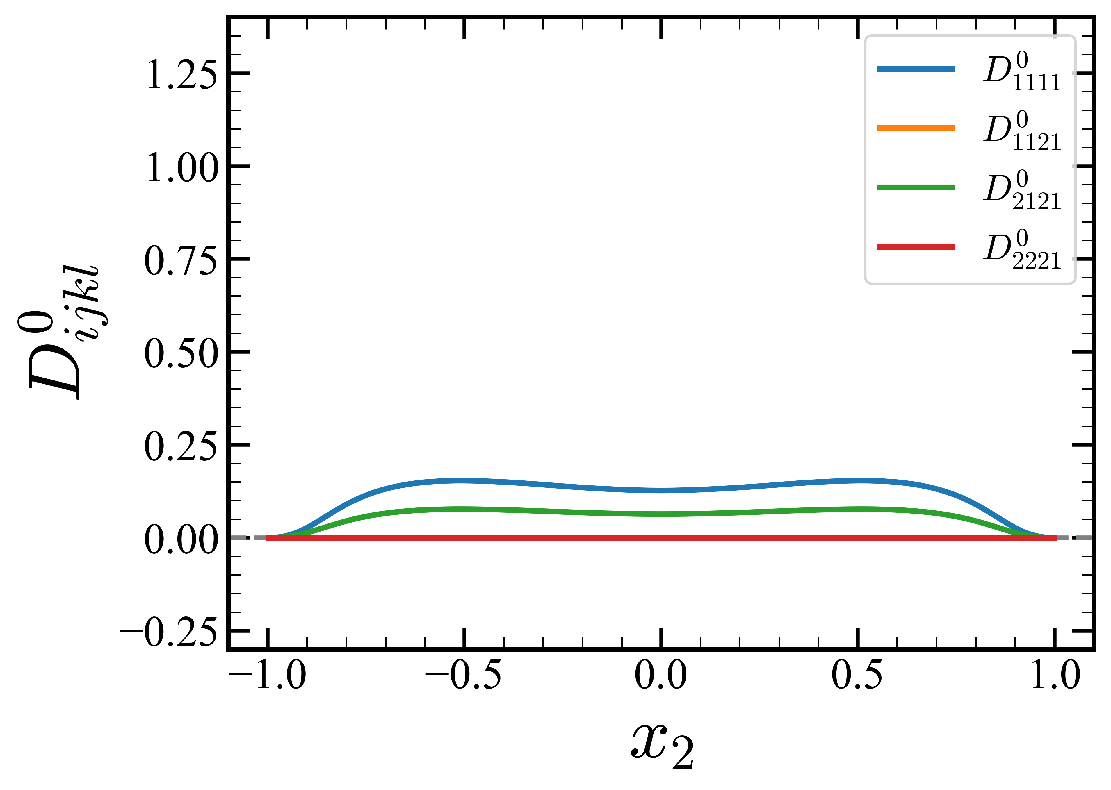
(b) Boussinesq

Figure 6: Comparison of the measured eddy viscosity elements $D^{0}_{1111}$ (blue line), $D^{0}_{1121}$ (orange line), $D^{0}_{2121}$ (green line), and $D^{0}_{2221}$ (red line) to the Boussinesq approximation.

As we discussed since flow structures and thus momentum mixing is similar between the channel flow and the attached boundary layers, we can use the measured eddy viscosity anisotropy in the former setting to identify important eddy viscosity components for the latter setting. To this end, we present in Appendix D a scaling analysis of various gradients contributing to the Reynolds stress tensor. Combining this analysis with the measured order of magnitude of each eddy viscosity component that acts as a pre-factor multiplying components of the velocity gradient tensor, we identify the key eddy viscosity components that contribute dominantly to the Reynolds stress tensor budget. Based on our analysis we identify $D_{1111}$, $D_{1121}$, $D_{2121}$, and $D_{2221}$ as the key four, out of 16, dominant eddy viscosity components for 2D spatially developing turbulent boundary layers.

Motivated by this example, we next examine the identified anisotropy against the Bousinesq approximation. When we cast the Boussinesq approximation to our tensorial representation, the components in the eddy viscosity tensor are in ratio of 0, 1, or 2 to the standard eddy viscosity $\nu_{T}$. For instance, the four elements are prescribed with following ratios; $D_{1111}=2\nu_{T}$, $D_{1121}=0$, $D_{2121}=\nu_{T}$, and $D_{2221}=0$. Figure 6 shows the comparison of these eddy viscosity components to the Boussinesq approximation. In Figure 6(a), we show the measured four elements using our MFM calculation. In Figure 6(b) we set the standard eddy viscosity to the MFM-measured leading-order value, $\nu_{T}=D^{0}_{2121}$ and prescribe the other components with the ratio to $\nu_{T}$. As shown in the figure, a huge anisotropy is observed not only among all elements but specificallty among these four critical elements, and the ratio of these plots can locally go up to hundreds. We conclude that, while $D_{2121}$ is the most important eddy viscosity component for parallel and semi-parallel flows, the presence of small non-parallel effects could lead to significant influence of anisotropy in momentum transport in wall bounded flows.

Lastly, we point that there have been attempts to include the anisotropy in RANS such as Spalart-Allmaras model with quadratic constitutive relation (SA-QCR) (Spalart, 2000; Mani et al., 2013; Rumsey et al., 2020). However, examining our results suggest that these models do not captured the level of the anisotropy that MFM measured. For instance, SA-QCR still prescribes $D_{1111}=2\nu_{T}$ and the anisotropy is not yet introduced in needed directions.

3.3 Dependence on the rate of rotation

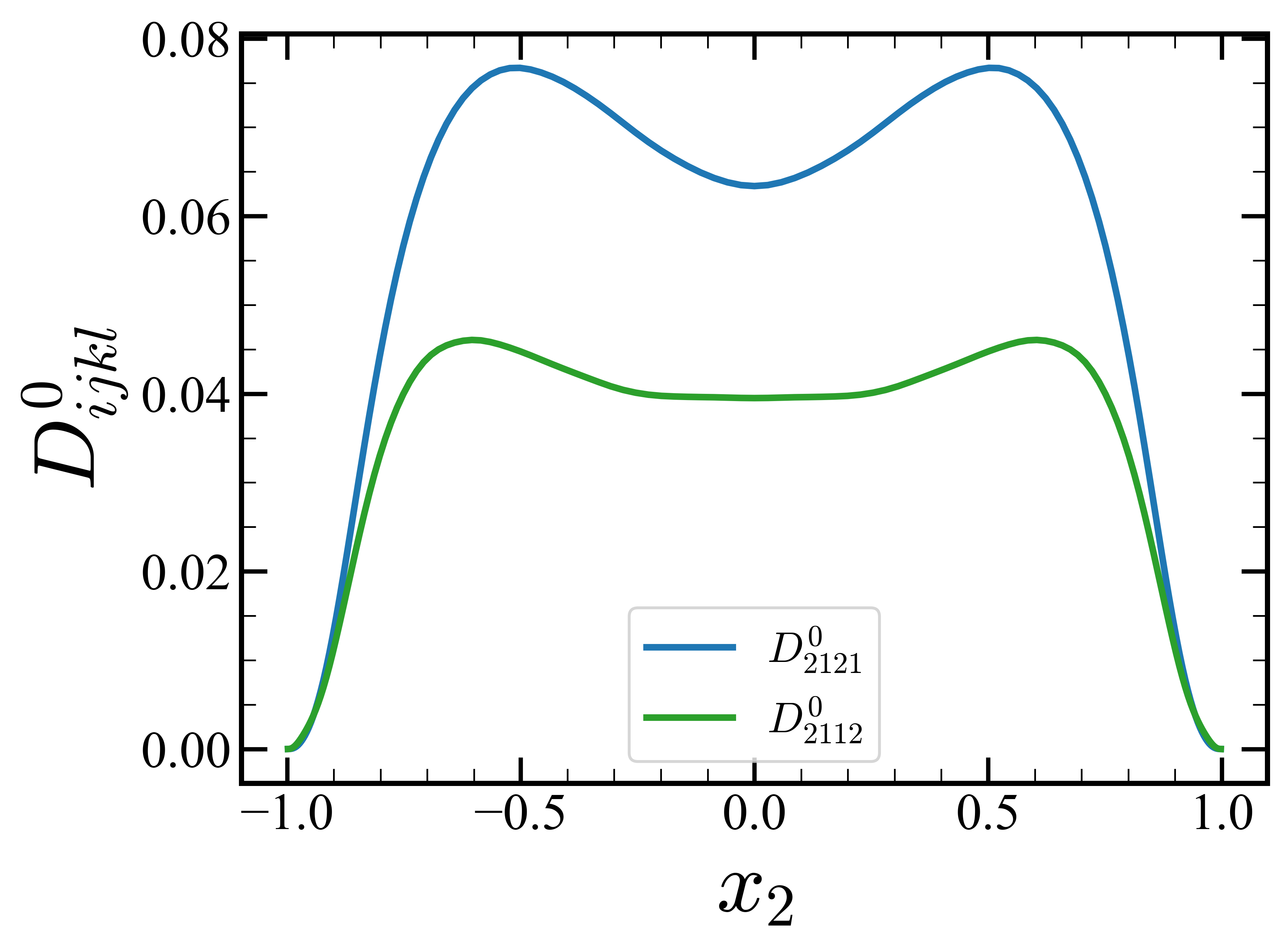
Figure 7: Comparison of $D^{0}_{2121}$ (blue line) and $D^{0}_{2112}$ (green line).

One of the major explicit assumptions in the Boussinesq approximation is that the Reynolds stress is dependent only on the rate of strain $S_{ij}$ and not on the rate of rotation $\omega_{ij}$. With our eddy viscosity tensor notation, this indicates that $D^{0}_{ijkl}=D^{0}_{ijlk}$ because under this condition, each Reynolds stress component, $\overline{u^{\prime}_{i}u^{\prime}_{j}}$, would be equally sensitive to both $\partial U_{l}/\partial x_{k}$ and $\partial U_{k}/\partial x_{l}$, and thus is a function of the summation $\partial U_{l}/\partial x_{k}+\partial U_{k}/\partial x_{l}$, which is $2S_{kl}$. One can verify that under this condition the inner product $D^{0}_{ijkl}\omega_{lk}$ would be identically zero. because the inner product of the anti-symmetric tensor, the rate of rotation, to the symmetric tensor is zero. However, our measurement of the leading-order eddy viscosity tensor invalidates the relation. Figure 7 shows the comparison between $D^{0}_{2121}$ and $D^{0}_{2112}$. These two components have the same sign and their qualitative shape is similar, but the magnitudes are drastically different. In order for the Boussinesq assumption to be true, the two values must be identical. This highlight an important conclusion: the mean rotation can cause significant Reynolds stress even at the leading-order. Likewise, we reach the same conclusion with the case of $D^{0}_{ij13}$ and $D^{0}_{ij23}$.

3.4 Leading-order Reynolds stress

(a) $D^{0}_{1121}$

(b) $D^{0}_{1221}$

(c) $D^{0}_{2121}$

(d) $D^{0}_{2221}$

(e) $D^{0}_{3321}$

Figure 8: Reynolds stresses constructed by the leading-order eddy viscosity tensor associated with (a) $D^{0}_{1121}$, (b) $D^{0}_{1221}$, (c) $D^{0}_{2121}$, (d) $D^{0}_{2221}$, and (e) $D^{0}_{3321}$: green dotted line, the reconstructed Reynolds stress by the leading-order eddy viscosity tensor; blue solid line, the DNS data.

In Section 3.1, we computed a RANS solution using $D^{0}_{2121}$ and compare the solution to that of the DNS to assess appropriateness of the leading-order eddy viscosity for prediction of the mean velocity profile. Another way to make this assessment is to reconstruct Reynolds stress using the computed eddy viscosity tensor and compare it to the Reynolds stress of DNS. This way, we can assess some other components in $D^{0}_{ijkl}$. The Reynolds stress in the channel flow can be represented in the following way: $\overline{u^{\prime}_{i}u^{\prime}_{j}}=-D^{0}_{ij21}{\partial U_{1}}/{\partial x_{2}}$. With the leading-order eddy viscosity tensor $D^{0}_{ij21}$ computed using MFM and with the mean velocity gradient ${\partial U_{1}}/{\partial x_{2}}$ measured from the DNS data, we construct the Reynolds stress $\overline{u^{\prime}_{i}u^{\prime}_{j}}$.

Figure 8 shows the five reconstructed Reynolds stresses associated with the RANS prediction of the channel flow, in comparison with the Reynolds stresses from the DNS data. There are three important observations with the Reynolds stresses that are reconstructed with the leading-order eddy viscosity tensor. The first finding is that while the Reynolds stresses reconstructed using the leading-order eddy viscosity show similar qualitative trends and orders of magnitudes to those from DNS, there’s still a noticeable difference between the two. This difference is likely due to the leading-order truncation of the eddy viscosity operator. Among the various Reynolds stresses, only $\overline{u^{\prime}_{2}u^{\prime}_{1}}$ is accurately constructed. This suggests that this specific component is influenced by local mean gradients, while the other components show nonlocal dependence at least in a portion of the domain.

The next important observation is that constructed Reynolds stresses from the leading-order eddy viscosity are not symmetric. This asymmetry error is entirely due to the truncated representation of the eddy viscosity to its local term, i.e. the leading term in Equation 11. As we shall see, inclusion of the full nonlocal eddy viscosity will eliminate this error. However, the fact that the leading-order $\overline{u^{\prime}_{2}u^{\prime}_{1}}$ match the DNS, substantially better than $\overline{u^{\prime}_{1}u^{\prime}_{2}}$ indicates that the former Reynolds stress is more local while the latter has substantial nonlocal sensitivity to the mean velocity gradient. While we do not have an intuitive explanation for this observation, we note the coincidence that the former Reynolds stress, represents flux of an active mean momentum component in the direction where its gradients are active. The only way that the latter Reynolds stress could be generated in this setting is through pressure coupling, whose fluctuations are known to nonlocally depend on velocity fluctuations.

Lastly, we observe that is that the leading-order model cannot approximate the nonzero centerline value, where the velocity gradient is zero due to the symmetry of the channel flow. But, since the trace part of the Reynolds stress at the centerline is nonzero, the nonlocality needs to be included in eddy viscosity to enable prediction of the centerline value. In Section 3.5, we examine the eddy viscosity and the Reynolds stress further by including the nonlocality.

3.5 Positive Definiteness

It is noted that the Reynolds stress is a positive semi-definite tensor (Du Vachat, 1977; Schumann, 1977). Therefore, we often require eddy viscosity to satisfy the same condition as done in the Boussinesq approximation with $\nu_{T}\geq 0$ (Speziale et al., 1994). In this section, we discuss whether this condition holds for our leading-order eddy viscosity tensor $D^{0}_{ijkl}$ as well.

The positive definiteness of the eddy viscosity is closely related to the mean kinetic energy equation, which is the following:

$$\frac{\partial}{\partial t}\left(\frac{U_{i}U_{i}}{2}\right)+U_{j}\frac{\partial}{\partial x_{j}}\left(\frac{U_{i}U_{i}}{2}\right) =\frac{\partial}{\partial x_{j}}\left(-\frac{P}{\rho}U_{j}\right)+\nu\frac{\partial^{2}U_{i}U_{i}/2}{\partial x_{j}\partial x_{j}}$$ (15)

$$-\nu\frac{\partial U_{i}}{\partial x_{j}}\frac{\partial U_{i}}{\partial x_{j}}-\frac{\partial}{\partial x_{j}}\left(U_{i}\overline{u_{j}^{\prime}u_{i}^{\prime}}\right)+\overline{u_{j}^{\prime}u_{i}^{\prime}}\frac{\partial U_{i}}{\partial x_{j}}.$$ (16)

The last term in Equation 16 is the negative of turbulent kinetic energy production. It is well-known that this term drains the kinetic energy from the mean flow via interactions of the mean shear and the turbulent fluctuations, and provide energy to the turbulence production. We denote the turbulent kinetic energy as $P_{k}=-\overline{u_{j}^{\prime}u_{i}^{\prime}}\frac{\partial U_{i}}{\partial x_{j}}$. In all statistically stationary flows, the volumetric integral of $P_{k}$ must be non-negative. There are certain cases such as the separation of the shear layer where $P_{k}$ is locally negative, but even for those cases, the turbulent production is positive for the most of the domain (Cimarelli et al., 2019). The volumetric integral condition for $P_{k}$ can be expressed using our generalized eddy viscosity expression in Equation 1.

$$\int{P_{k}}\differential[3]{\mathbf{x}} =\int-\overline{u_{j}^{\prime}u_{i}^{\prime}}\left.\frac{\partial U_{i}}{\partial x_{j}}\right|_{\mathbf{x}}\differential[3]{\mathbf{x}}$$ (17)

$$=\int\int D_{ijkl}(\mathbf{x},\mathbf{y})\left.\partialderivative{U_{l}}{x_{k}}\right|_{\mathbf{y}}\left.\frac{\partial U_{i}}{\partial x_{j}}\right|_{\mathbf{x}}\differential[3]{\mathbf{y}}\differential[3]{\mathbf{x}}$$ (18)

Furthermore, this condition is also required for well-posedness and numerical robustness of the simulation. Similar work has been done by Milani (2020) in the context of the scalar transport.

We can further reduce the Equation 18 using our leading-order eddy viscosity tensor as the closure model, then the production term becomes:

$$\int{P_{k}}\differential[3]{\mathbf{x}}\simeq\int D^{0}_{ijkl}(\mathbf{x})\left.\partialderivative{U_{l}}{x_{k}}\right|_{\mathbf{x}}\left.\frac{\partial U_{i}}{\partial x_{j}}\right|_{\mathbf{x}}\differential[3]{\mathbf{x}}$$ (19)

Since the operator is now local, this implies that positive definiteness must be satisfied for each point. Then, $D^{0}_{ijkl}\frac{\partial U_{j}}{\partial x_{i}}\frac{\partial U_{l}}{\partial x_{k}}\geq 0$ must also be satisfied. In other word, the quadratic form of the eddy viscosity tensor is non-negative. Therefore, we can conclude that anisotropic eddy viscosity tensor is positive semi-definite.

Using our MFM measurement of the eddy viscosity, we can examine whether a local model from the truncated Kramer-Moyal expansion satisfies the positive semi-definite condition. If the positive semi-definite condition is not satisfied, it is an indication that the local truncation is not valid and nonlocality is needed for the positive definiteness condition.

To test the positive semi-definiteness of the eddy viscosity tensor, we flatten the eddy viscosity tensor and the velocity gradient. Then, the turbulent production becomes $D^{0}_{ijkl}\frac{\partial U_{j}}{\partial x_{i}}\frac{\partial U_{l}}{\partial x_{k}}=\mathbf{z}^{T}\mathbf{D}\mathbf{z}$ where $\mathbf{z}$ is the flattened velocity gradient $[{\partial U_{1}}/{\partial x_{1}}~{}{\partial U_{2}}/{\partial x_{1}}~{}{\partial U_{1}}/{\partial x_{2}}~{}{\partial U_{2}}/{\partial x_{2}}]^{T}$ and where $\mathbf{D}$ is the following matrix:

$$\mathbf{D}=\begin{bmatrix}D^{0}_{1111}&D^{0}_{1112}&D^{0}_{1121}&D^{0}_{1122}\\ D^{0}_{1211}&D^{0}_{1212}&D^{0}_{1221}&D^{0}_{1222}\\ D^{0}_{2111}&D^{0}_{2112}&D^{0}_{2121}&D^{0}_{2122}\\ D^{0}_{2211}&D^{0}_{2212}&D^{0}_{2221}&D^{0}_{2222}\\ \end{bmatrix}$$

It is well known that a symmetric $\mathbf{D}$ is positive semi-definite if and only if $\mathbf{z}^{T}\mathbf{D}\mathbf{z}\geq 0$ for all real vector $\mathbf{z}$. However, for our case, $\mathbf{D}$ is non-symmetric and $\mathbf{z}$ is limited to only certain value due to the incompressible condition. Therefore, we modified the quantity of interest. First of all, instead of the non-symmetric matrix $\mathbf{D}$, we look at the positive definiteness of $\mathbf{D}+\mathbf{D}^{T}$. If $\mathbf{D}+\mathbf{D}^{T}$ is positive semi-definite, $\mathbf{z}^{T}\mathbf{D}\mathbf{z}\geq 0$ also holds (Milani, 2020). Secondly, since the flow system is incompressible, $\mathbf{z}$ is limited to certain values satisfying ${\partial U_{2}}/{\partial x_{2}}=-{\partial U_{1}}/{\partial x_{1}}$. To expand the column vector multiplied to matrix $\mathbf{D}$ to every nonzero real column vector, we must embed the incompressibility condition to the matrix $\mathbf{D}$. We define $\mathbf{z}=\mathbf{C}\mathbf{z^{*}}$ where $\mathbf{z^{*}}$ is the reduced flattened velocity gradient $[{\partial U_{1}}/{\partial x_{1}}~{}{\partial U_{2}}/{\partial x_{1}}~{}{\partial U_{1}}/{\partial x_{2}}]^{T}$ and $\mathbf{C}$ is the following matrix:

$$\mathbf{C}=\begin{bmatrix}1&0&0\\ 0&1&0\\ 0&0&1\\ -1&0&0\\ \end{bmatrix}$$

Using this definition, $\mathbf{z}^{T}\mathbf{D}\mathbf{z}$ becomes $\mathbf{z^{*}}^{T}\mathbf{C}^{T}\mathbf{D}\mathbf{C}\mathbf{z^{*}}$. Combining these two methods, we conclude that the eddy viscosity tensor is positive semi-definite when all the eigenvalues of the matrix $\mathbf{C}\left(\mathbf{D}+\mathbf{D}^{T}\right)\mathbf{C}^{T}$ is non-negative. We computed the smallest eigenvalue of this matrix at each $x_{2}$. The resulting plot is shown in Figure 9. As shown, except for the thin zones near the wall, we see that the eigenvalues are positive, hence the eddy viscosity tensor is positive definite. Near the wall, however, the eigenvalues become negative, indicating that the leading term is not sufficient to capture the positive semi-definiteness of the eddy viscosity. In other words, this negativity occurs due to the local truncation of the eddy viscosity tensor and therefore nonlocality should be incorporated to make the eddy viscosity positive semi-definite.

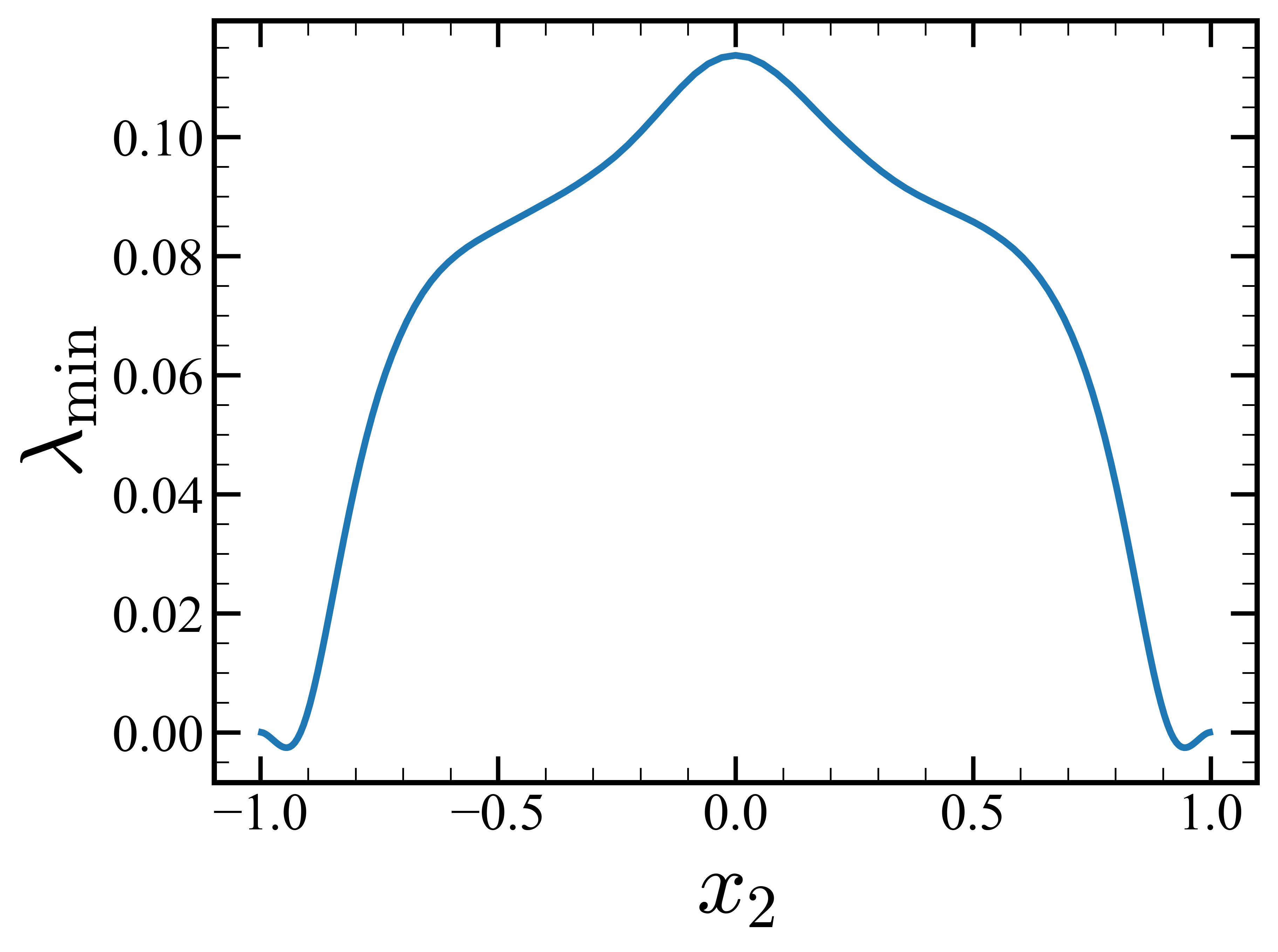
Figure 9: The minimum eigenvalue of the matrix $\mathbf{C}\left(\mathbf{D}+\mathbf{D}^{T}\right)\mathbf{C}^{T}$.

4 Nonlocality Analysis

In Section 3.3, we concluded that aside from $\overline{u^{\prime}_{2}u^{\prime}_{1}}$, capturing other components of the Reynolds stress field requires inclusion of nonlocal terms in the eddy viscosity operator. To further understand the non-Boussinesq effect in this section, we investigate the full eddy viscosity kernel $D_{ijkl}\left(x_{2},y_{2}\right)$ in Equation 8 to assess the nonlocality of the eddy viscosity.

4.1 Nonlocality

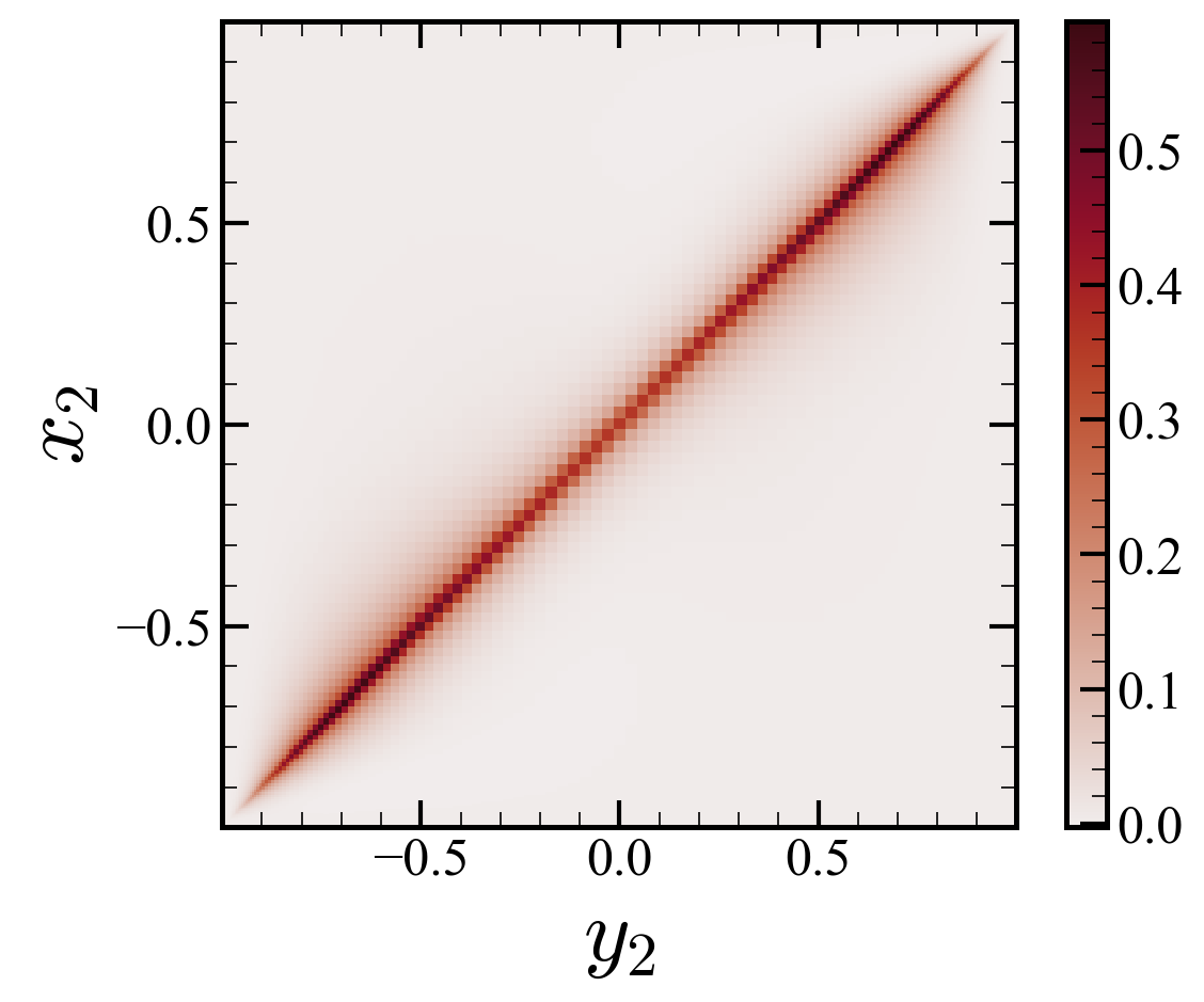
(a) $D_{2121}$

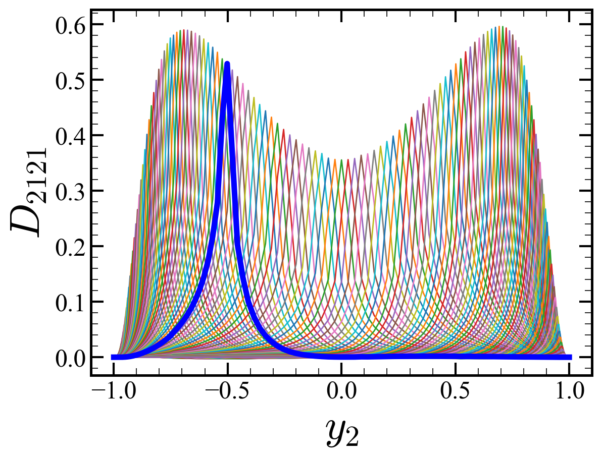
(b) $D_{2121}$

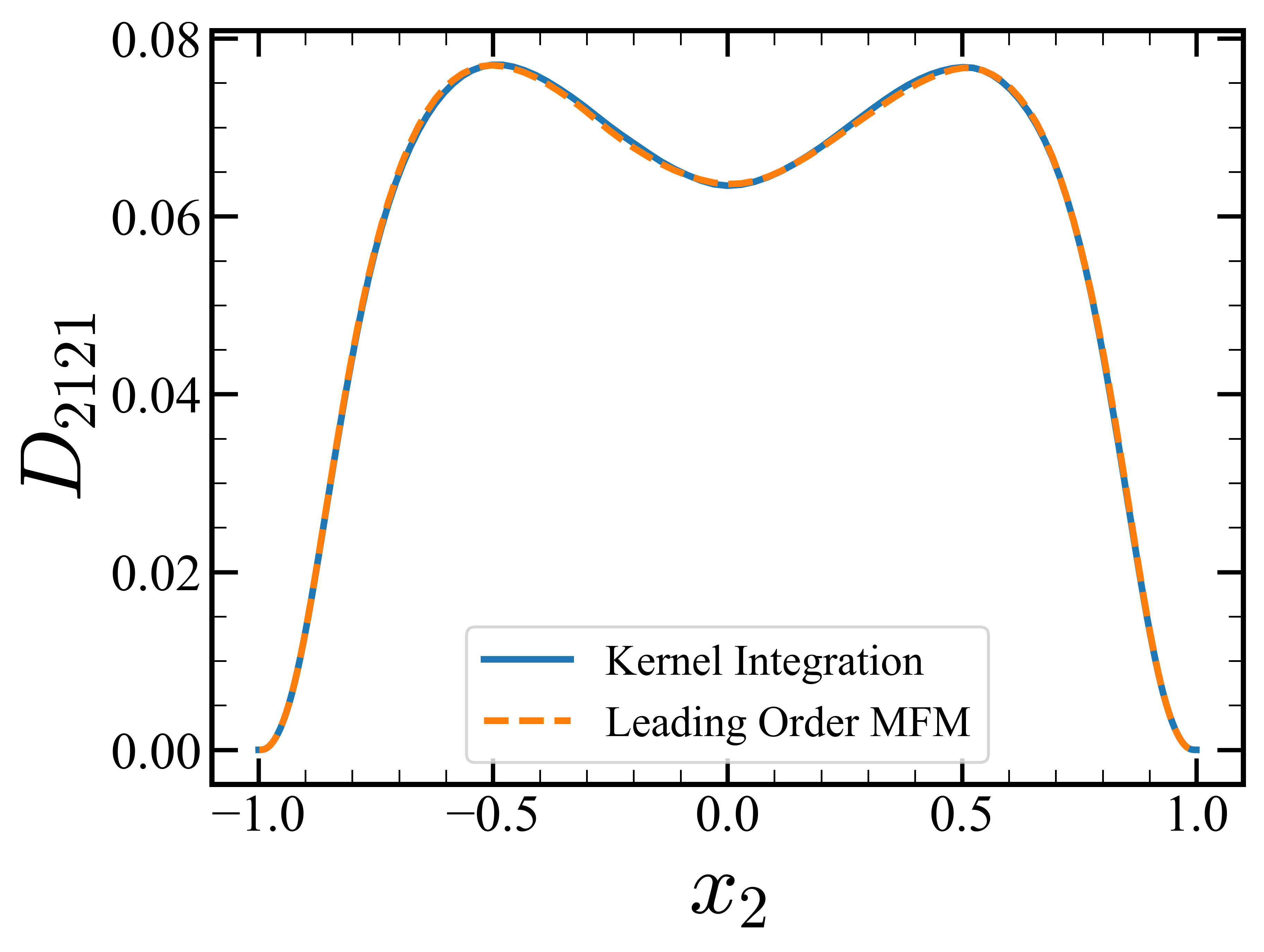
(c) $\int D_{2121}\mathrm{d}y_{2}$

Figure 10: Distribution of $D_{2121}$: (a) contour plot of $D_{2121}$, (b) $D_{2121}\left(x_{2}=x_{2}^{*},y_{2}\right)$ with various $x_{2}^{*}$ where the blue line is at $x_{2}^{*}=0.502$, and (c) the blue solid line, $\int D_{2121}\mathrm{d}y_{2}$ and the orange dashed line, $D^{0}_{2121}$.

Figure 10 shows the full eddy viscosity kernel representation of the $D_{2121}$ component. Each point in Figure 10(a) represents the effect of the velocity gradient at the location $y_{2}$ to the Reynolds stress at the location $x_{2}$. The distribution of $D_{2121}$ is quite narrow and confined to $x_{2}\sim y_{2}$, indicating the locality of this eddy viscosity. At a given location $x_{2}$, we can visualize how much contribution the remote velocity gradient at different location $y_{2}$ makes to the Reynolds stress at the location $x_{2}$.

For instance, in Figure 10(b), the thick blue line represents $D_{2121}\left(x_{2}=0.502,y_{2}\right)$ and the distribution indicates the effects of the velocity gradient nearby. If the Boussinesq approximation holds, a delta function around $y_{2}=0.502$ is expected. In the figure, even though the plotted profile is not identical to a Dirac delta function, $D_{2121}\left(x_{2}=0.502,y_{2}\right)$ shows concentrated behavior around $y_{2}=0.502$. The rest of the plots in Figure 10(b) shows $D_{2121}\left(x_{2}=x_{2}^{*},y_{2}\right)$ at other $x_{2}^{*}$. Overall, our narrow banded results indicate that $D_{2121}$ is highly local throughout the domain, with small deviation to the Boussinesq approximation. Such locality explains the earlier conclusion in Section 3 that a leading-order eddy viscosity is reasonable for this parallel flow.

In addition, Figure 10(c) is comparing the results of kernel integration $\int{D_{2121}\mathrm{d}y_{2}}$ and the leading-order eddy viscosity tensor component $D^{0}_{2121}$. The definition of $D^{0}_{2121}$ is the leading-order moment of the eddy viscosity kernel $D_{2121}$. In other word, the integration of the kernel $\int{D_{2121}\mathrm{d}y_{2}}$ must match the eddy viscosity tensor $D^{0}_{2121}$. Figure 10(c) shows that the two results are collapsing verifying that our two different MFM measurements, MFM for $D^{0}_{ijkl}$ and MFM for $D_{2121}$ show consistent result.

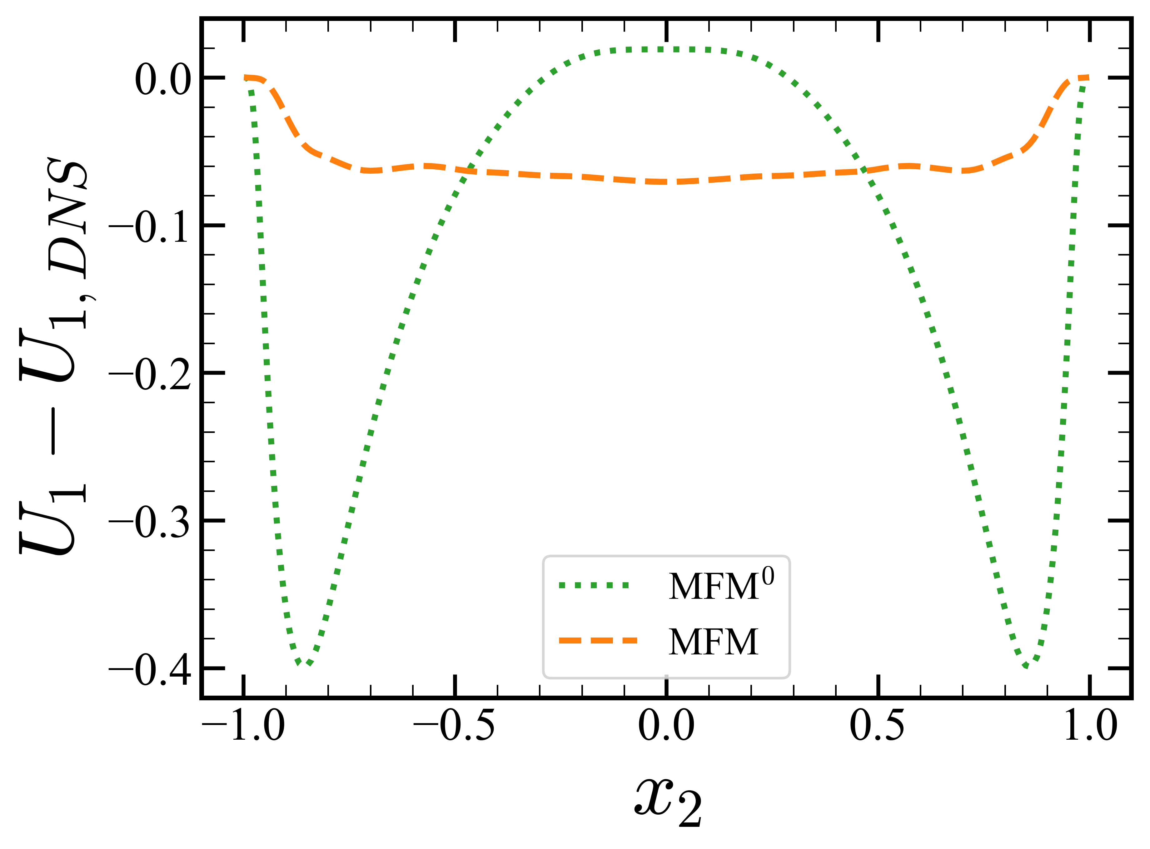
Figure 11: Error in RANS prediction of the streamwise velocity using eddy viscosity tensor $D^{0}_{2121}$ (denoted as MFM⁰) and eddy viscosity kernel $D_{2121}$ (denoted as MFM), $U_{1}-U_{1,\mathrm{DNS}}$; the dotted green line, $U_{1}$ predicted with $D^{0}_{2121}$ and the dashed orange line, $U_{1}$ predicted with $D_{2121}$.

In Section 3, we demonstrated that the leading-order eddy viscosity alone can predict a highly accurate RANS solution for the channel mean velocity with the prediction error around 1%. This error can be furture reduced by including the nonlocality using the full kernel representation of the eddy viscosity. Figure 11 shows the two RANS results, one obtained using the leading-order eddy viscosity $D^{0}_{2121}$ and the other obtained using eddy viscosity kernel $D_{2121}$. Analytically, the full measurement of the kernel is expected to provide the RANS solution that is identical to the averaged DNS result. In our simulation, small errors are due to statistical noise that we expect to resolve with a larger data set. Still, the kernel result is significantly better than the leading-order result, indicating that even the RANS simulation of the channel, which is highly local, can be improved using a nonlocal model.

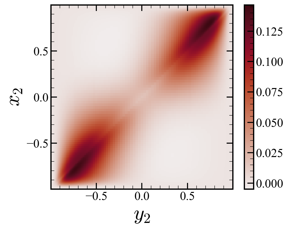
(a) $D_{1221}$

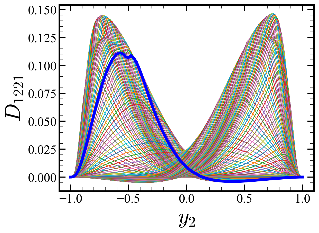
(b) $D_{1221}$

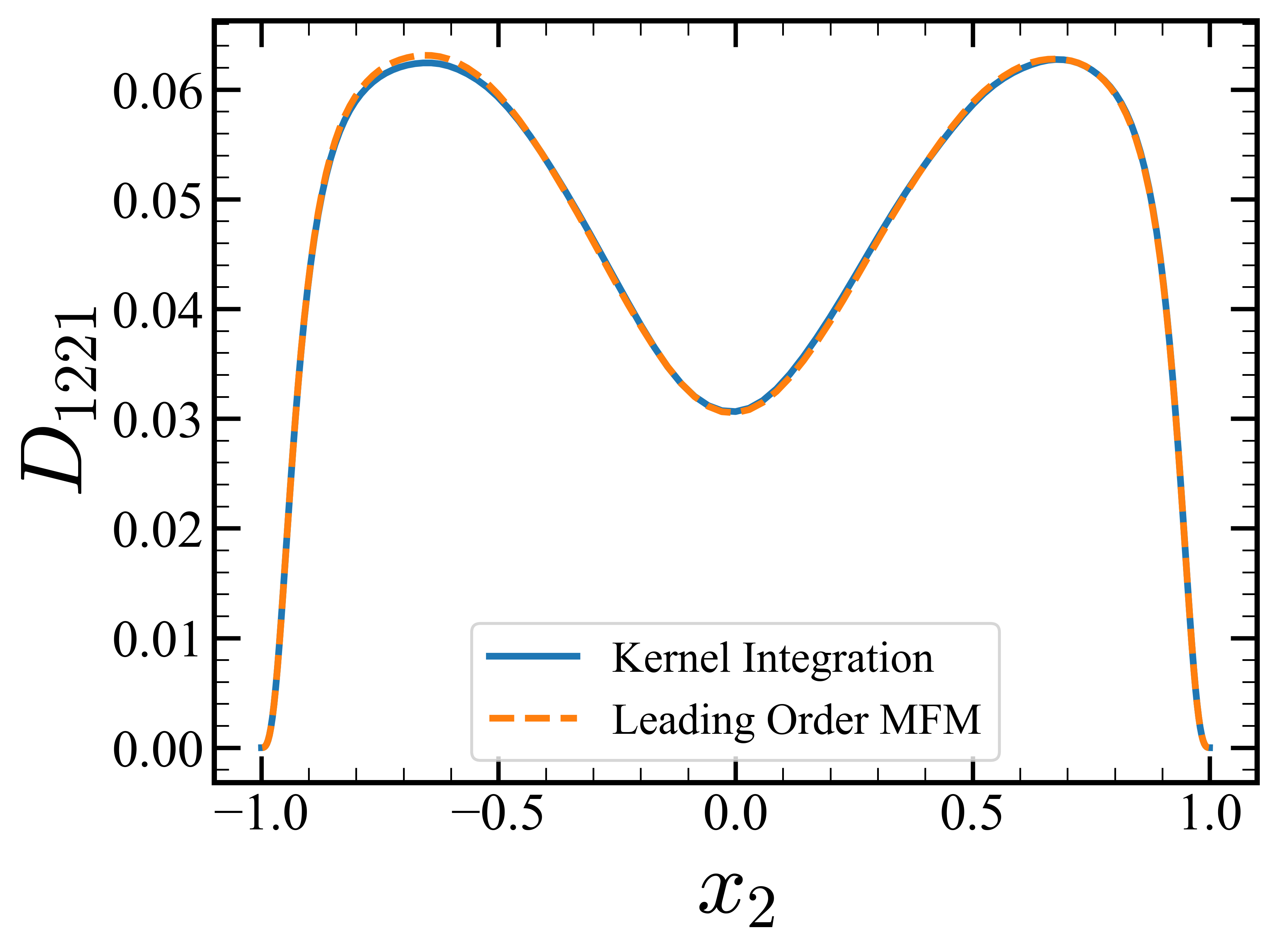
(c) $\int D_{1221}\mathrm{d}y_{2}$

Figure 12: Distribution of $D_{1221}$: (a) contour plot of $D_{1221}$, (b) $D_{1221}\left(x_{2}=x_{2}^{*},y_{2}\right)$ with various $x_{2}^{*}$ where the blue line is at $x_{2}^{*}=0.502$, and (c) blue solid line, $\int D_{1221}\mathrm{d}y_{2}$ and orange dashed line, $D^{0}_{1221}$.

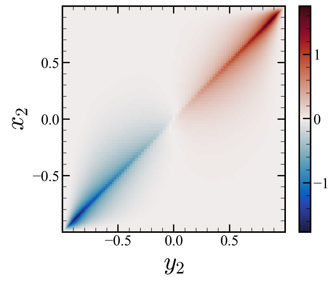
(a) $D_{1121}$

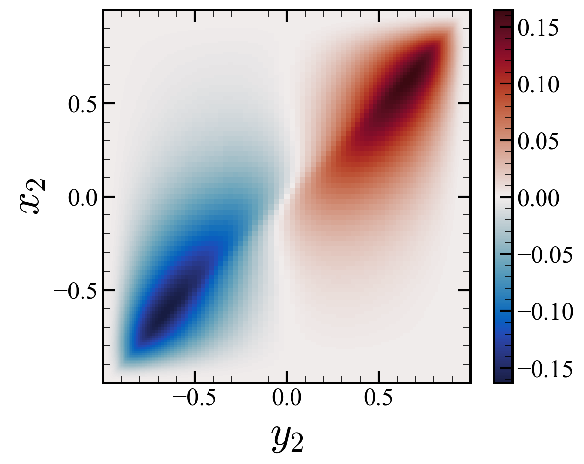
(b) $D_{2221}$

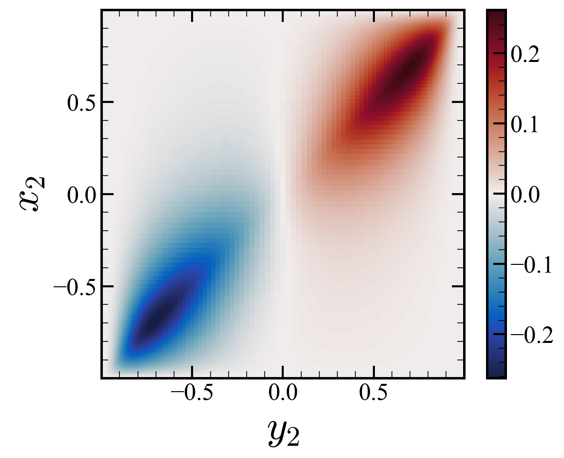
(c) $D_{3321}$

Figure 13: Distribution of nonzero $D_{ij21}$ where (a) $D_{1121}$, (b) $D_{2221}$, and (c) $D_{3321}$.

Next, we assess nonlocality of other components of $D_{ijkl}$ by examining the corresponding kernels. For example, the eddy viscosity kernel $D_{1221}$ (Figure 12) is widespread and shows significant nonlocality, invalidating the intrinsic assumption in the Boussinesq approximation. The level of nonlocality is drastic such that the velocity gradient at one half of the channel may affect the Reynolds stress at the other half of the domain. Moreover, the shape of $D_{2121}$ differs from $D_{1221}$, implying the non-universality of the kernel profile across different components of eddy diffusivity. Furthermore, the differences in the kernel shape between $D_{2121}$ and $D_{1221}$, clarifies why a truncated eddy viscosity operator based on the leading term of its Kramer-Moyal expansion can lead to asymmetric Reynolds stresses. Figure 13 shows the additional three nonzero eddy viscosity kernel $D_{1121}$, $D_{2221}$, and $D_{3321}$. The rest of the components are zero due to channel symmetry. These three kernels correspond to the trace part of the eddy viscosity kernel and are also highly nonlocal.

4.2 Revisit of Reynolds stress

(a) $D_{1121}$

(b) $D_{1221}$

(c) $D_{2121}$

(d) $D_{2221}$

(e) $D_{3321}$

Figure 14: Reynolds stresses constructed by the leading-order eddy viscosity tensor and the eddy viscosity kernel associated with (a) $D_{1121}$, (b) $D_{1221}$, (c) $D_{2121}$, (d) $D_{2221}$, and (e) $D_{3321}$: orange dashed line, the reconstructed Reynolds stress by the eddy viscosity kernel; green dotted line, the reconstructed Reynolds stress by the leading-order eddy viscosity tensor; blue solid line, the DNS data.

Lastly, we revisit the Reynolds stress reconstruction with the inclusion the effects of the nonlocality. Figure 14 shows three different ways of constructing the Reynolds stresses. The first shown in the orange dashed line is the reconstructed Reynolds stress by the eddy viscosity kernel from MFM and the mean velocity gradient from DNS. The second shown in green dotted line is the reconstructed Reynolds stress by the leading-order eddy viscosity tensor from MFM and the mean velocity gradient from DNS. The last one is from the mean DNS data shown in blue solid line. The leading-order result and the mean DNS data are shown before in Figure 8.

Unlike the leading-order analysis, the results from the full kernel eddy viscosity matches very well to the DNS data. These plots verify our computational method yielding two findings. First, with full kernels, the Reynolds stresses recover the symmetry that was lost in the leading-order approximation. Only $D_{2121}$, which is quite narrow banded, is applicable for the local approximation. Hence, this leads to the symmetry breakage after leading-order approximation. Second, now we can capture the nonzero Reynolds stress at the channel centerline. Thus, the measured nonlocal eddy viscosity allows prediction of non-zero Reynolds stresses near the centerline, whereas the leading-order approximation fails to do so.

4.3 Revisit of Positive Definiteness

In Section 4.5, we discuss the positive definiteness of the local eddy viscosity tensor $D^{0}_{ijkl}$. Due to the leading-order truncation of the eddy viscosity kernel, $D_{ijkl}$, our result indicated that the local eddy viscosity tensor was not positive definite near the walls. In this section, we introduce the full kernel and see if including the nonlocality restores the semi-positive definite condition.

Using the full eddy viscosity kernel expression and applying the fact that there exist only one nonzero velocity gradient in the turbulent channel flow, the turbulent production in Equation 18 can be written as the following:

$$\int P_{k}\mathrm{d}x_{2}=\int\int D_{2121}({x_{2}},{y_{2}})\frac{\partial U_{1}}{\partial y_{2}}\frac{\partial U_{1}}{\partial x_{2}}\mathrm{d}y_{2}\mathrm{d}x_{2}=\left[\frac{\partial U_{1}}{\partial x_{2}}\right]^{T}\left[D_{2121}\right]\left[\frac{\partial U_{1}}{\partial x_{2}}\right].$$

The far right term represents the discrete form of the expression, where $\left[\frac{\partial U_{1}}{\partial x_{2}}\right]$ represents any velocity gradient vector at each point in $x_{2}$ and $\left[D_{2121}\right]$ represents the discrete matrix value of $D_{2121}({x_{2}},{y_{2}})$. To make the turbulent production non-negative, the matrix $\left[D_{2121}\right]$ needs to be semi-positive definite. Likewise in Section 4.5, we computed eigenvalues of $\left[D_{2121}\right]+\left[D_{2121}\right]^{T}$ to determine the positive definiteness. The computed eigenvalues range from 0.00 to 7.58, indicating that the eddy viscosity kernel $D_{2121}$ is indeed semi-positive definite, recovering the stability condition that was lost by the leading-order truncation.

5 Conclusion

This study presents a quantification of non-Boussinesq effects in eddy viscosity in a subclass of turbulent wall-bounded flows. The presented analyses is systematically focused on two aspects: anisotropy and nonlocality of momentum mixing. To assess these effects and quantify the deviation from Boussinesq limit, we calculate the eddy viscosity of the turbulent channel flow at $\mathrm{Re}_{\tau}=180$ using a statistical technique that we recently developed called MFM. Using MFM, we quantify leading-order eddy viscosity tensor for the analysis of anisotropy and expand the research to quantification of eddy viscosity tensorial kernel for the analysis of nonlocality.

Our results indicate the following: (1) eddy viscosity is highly anisotropic with some elements orders of magnitude larger than the nominal eddy viscosity; (2) the Reynolds stresses reconstructed from this eddy viscosity depends not only on the mean rate of strain but also on mean rate of rotation; (3) leading-order eddy viscosity, which is obtained by neglecting higher spatial moments of the closure kernel, generates a non-symmetric Reynolds stress tensor; and (4) aside from the shear component of the Reynolds stress, $\overline{u^{\prime}_{2}u^{\prime}_{1}}$, the dependence of other components of Reynolds stress on mean velocity gradient is highly nonlocal at the level where some components of the Reynolds stress are influenced by the velocity gradient on the other half of the channel.

The exact measurement of the eddy viscosity of the channel flow has different implication for the RANS modeling of the parallel flow and that of the spatially developing boundary layers. For the parallel flow, only one Reynolds stress component and one velocity gradient are important; hence anisotropy does not influence the predictions of the solution as long as $D_{2121}$ is properly modeled. At the same time, not only the anisotropy but also nonlocality can be omitted for the channel flow since the spatial distribution of $D_{2121}(x_{2},y_{2})$ exhibits local distribution, as shown in our MFM measurement of the eddy viscosity kernel. These two findings explain why the Boussinesq approximation works well for parallel flows. However, our quantification suggests that this conclusion does not hold for spatially developing wall-bounded flows where the non-parallel effects become important. For instance, even a small gradient in the streamwise direction can have a non-neglible effect since $D_{1111}^{0}$ is very large compared to most of other eddy viscosity components. Our measurements reveal that the eddy viscosity is highly anisotropic and highly nonlocal, when it comes to components other than $D_{2121}$, indicating a clear need to include non-Boussinesq effects in RANS models.

While we focus on full nonlocal analysis in the $x_{2}$ direction, we do not consider nonlocal spatial effects in other directions and nonlocal temporal effects. Equation 8 is a reduced version of Equation 1 using leading-order moments in $x_{1}$, $x_{3}$, and $t$. These leading-order reductions are justified for channel flow since it is statistically homogeneous in these directions, and are expected to be qualitatively valid for systems with slow variation of turbulence in these directions. While it is possible to quantitatively assess such effects with MFM, we defer analysis of streamwise and spanwise nonlocality in eddy viscosity to a future study.

Appendix A Estimation of the convergence error

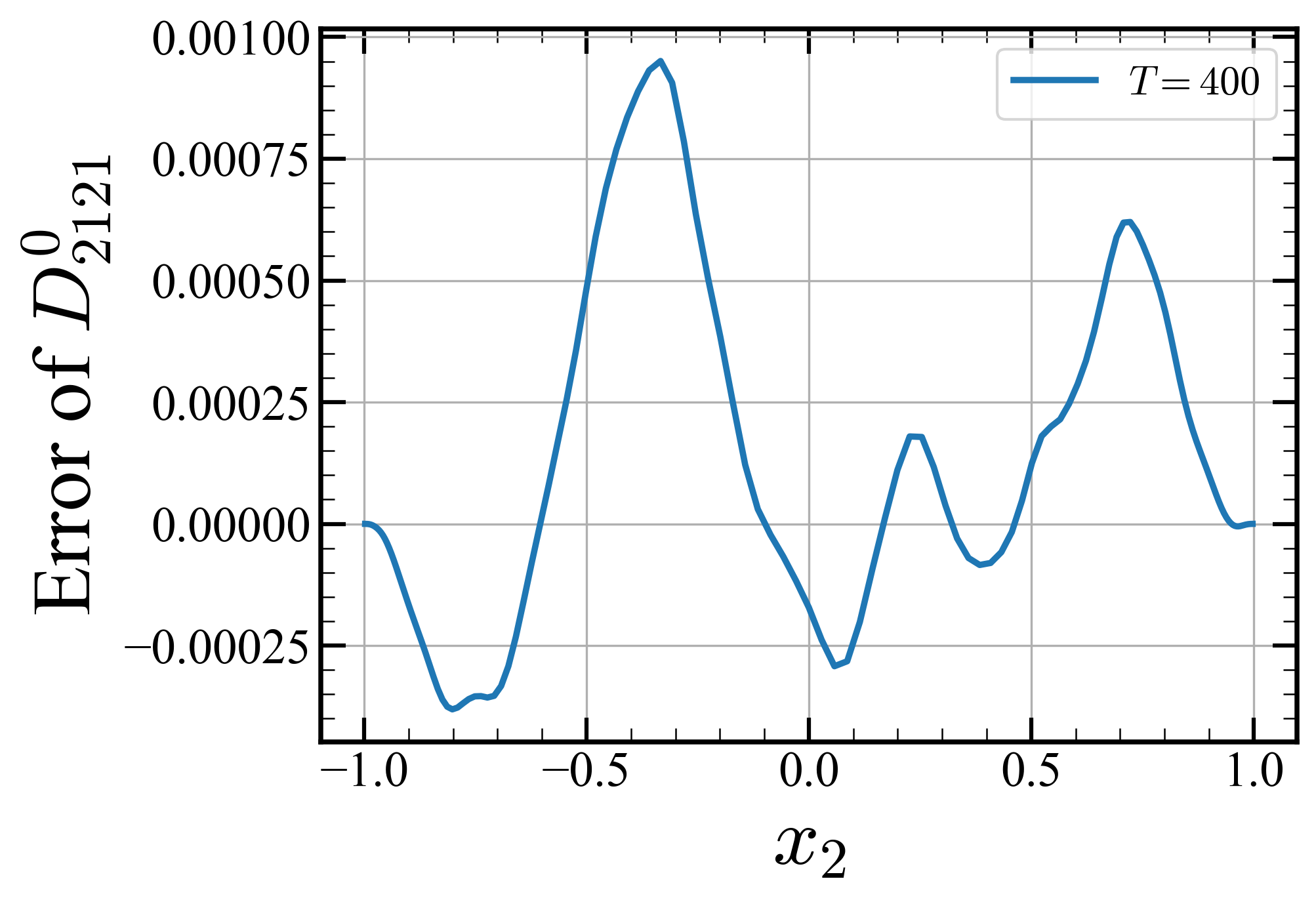
(a) Temporal convergence

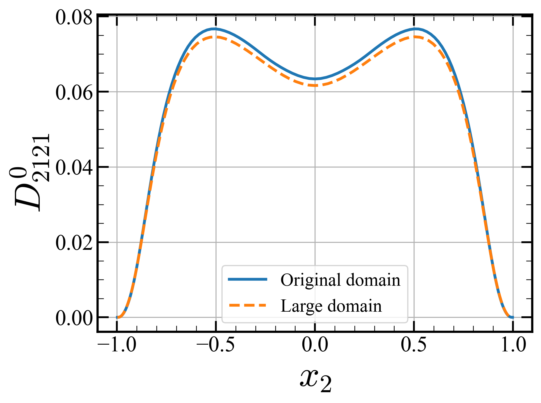
(b) Domain convergence

Figure 15: Convergence studies on $D^{0}_{2121}$; (a) $D^{0}_{2121}(T=400)-D^{0}_{2121}(T=850)$ where $T$ is normalized sampling time period; (b) $D^{0}_{2121}$ where the blue solid line is from the original domain (Table 1) and the orange dashed line is from the larger domain where domain length is twice larger in both $x_{1}$ and $x_{3}$ directions.

Figure 15 shows the convergence analysis of MFM results with respect to the spatio-temporal domain size. Figure 15(a) shows the estimated temporal error due to the finite time horizon of the MFM simulations. In our MFM studies we used a temporal sampling window of $T=850$ in eddy turnover time unit, which is substantially longer than simulation times typically used in the literature. We estimate the temporal convergence error by comparing $D^{0}_{2121}$ obtained from a shorter window, $T=400$, with that obtained from the full simulation. Based on the magnitude of the difference, shown in Figure 15(a), we estimate that the temporal convergence error, is about $1\%$.

In addition to the sampling time convergence study, we discuss the use of time dependent forcing. MFM restricts the forcing to be in the macroscopic space, the Reynolds-averaged space. For the channel flow, the forcing needs to be only a function of wall-normal direction, i.e. $s_{i}(x_{2})$, and hence, time independent. Therefore, the precise way of conducting the MFM analysis is to estimate the stationary forcing prior to the computation. This is problematic since it is difficult to know the forcing terms before the simulation. The remedy to this issue is to perform averages over ensembles, instead of using time averages. For a statistically stationary flow, the ensemble-averaged fields tend to time-constant fields as one increases the number of ensembles. Ensemble averages can then be accessed at each time step, in order to estimate $s_{i}(x_{2})$ according to the procedure described in Section 2.1.3. Since channel flow is statistically homogeneous in $x_{1}$ and $x_{3}$ directions, instead of creating new simulations, we used these directions for ensemble averaging. We then increased the number of independent ensembles by increasing the domain size in these directions. Figure 15(b) shows the computed $D^{0}_{2121}$ in two different domain sizes: one is the original domain size shown in Table 1 and the other is a larger domain which is twice bigger in both $x_{1}$ and $x_{3}$. The difference between these two plots are approximately $2\%$. This difference quantitatively represents the error committed by using a weakly time dependent forcings and finite domain size.

Appendix B Implementation for determining $D^{0}_{ijkl}$ in a periodic domain

MFM allows computation of every component in the leading-order eddy viscosity tensor $D^{0}_{ijkl}$ in Equation 12. In Section 2.2.2., we briefly explained how $D^{0}_{ij21}$ is determined via MFM with a forcing taht would maintain $V_{1}=x_{2}$ and $V_{2}=V_{3}=0$. For this case, boundary conditions and the initial condition are easily chosen to be compatible with the MFM instructions; for instance, periodic conditions in $x_{1}$ and $x_{3}$ direction and a Dirichlet condition in $x_{2}$ such as $v_{1}(x_{1},x_{2}=\pm 1,x_{3})=\pm 1$. The simple generalization of the forcing to other directions is $V_{n}=x_{m}$ and $V_{i\neq n}=0$ where $m$ and $n$ is not indices in the index notation, rather a choice of the forcing direction. However, such directional forcing is problematic in certain directions. For example, MFM of $V_{2}=x_{1}$ and $V_{1}=V_{3}=0$ forcing to compute $D_{ij12}$ has incompatible boundary conditions with the DNS solver since $V_{2}=x_{1}$ is not a periodic field in the streamwise direction . Therefore, to compute all the components of the eddy viscosity tensor, we modify the GMT to solve for the fluctuating part of the GMT variable $v_{i}^{\prime}$. We start from the GMT equations with forcing of $V_{n}=x_{m}$ and $V_{i\neq n}=0$ which gives a tensor $D^{0}_{ijmn}$ as shown in Equation 21. When we subtract the mean of the GMT equation from the GMT equation, the equation becomes the following:

$$\frac{\partial v_{i}^{\prime}}{\partial t}+\frac{\partial}{\partial x_{j}}\left(u_{j}v_{i}^{\prime}\right)=-\frac{\partial p}{\partial x_{i}}+\nu\frac{\partial^{2}v_{i}^{\prime}}{\partial x_{j}\partial x_{j}}+s_{i}-u_{m}\delta_{in}$$ (20)

At given $m$ and $n$, once we solve for the equation above, we can determine the nine of the eddy viscosity tensor by post-processing the results as Equation 21. Using various $m$ and $n$, we reveal all the element in the leading-order eddy viscosity tensor.

$$-\overline{u^{\prime}_{i}v^{\prime}_{j}}(x_{2})=\int_{{y_{2}}}D_{ijkl}({x_{2}},{y_{2}})\left.\frac{\partial V_{l}}{\partial x_{k}}\right|_{y_{2}}\mathrm{d}y_{2}\sim\int_{{y_{2}}}D_{ijmn}({x_{2}},{y_{2}})\mathrm{d}y_{2}=D^{0}_{ijmn}(x_{2})$$ (21)

There are multiple advantages of solving for GMT fluctuation equations. The first advantage is that the boundary condition is now compatible with the periodic conditions. Second, all the boundary conditions are easily set with a periodic condition or a Dirichet condition of $v_{i}^{\prime}=0$ at the boundary. With these two advantages, the solver become more systematic and simple.

Appendix C Leading-order eddy viscosity tensor

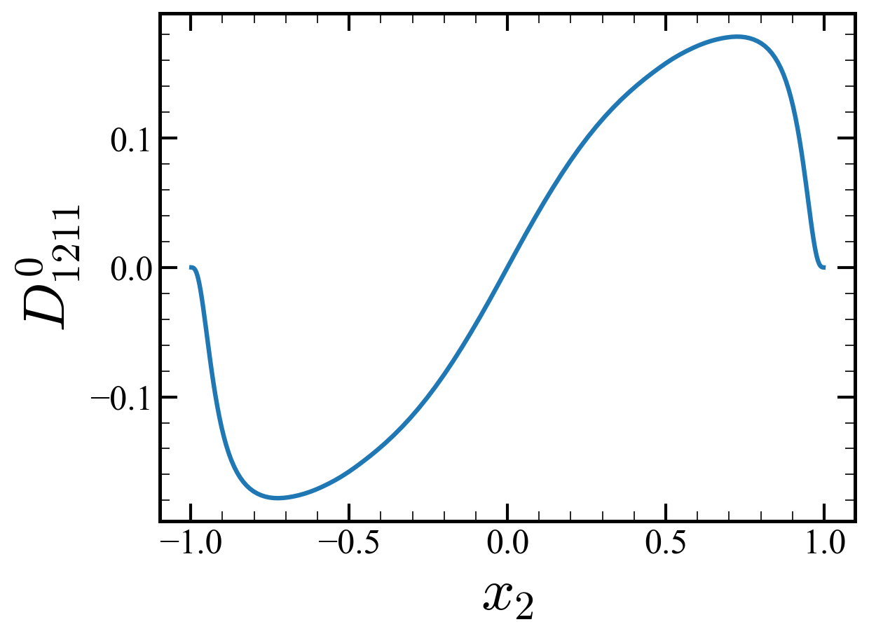
(a) $D_{1211}$

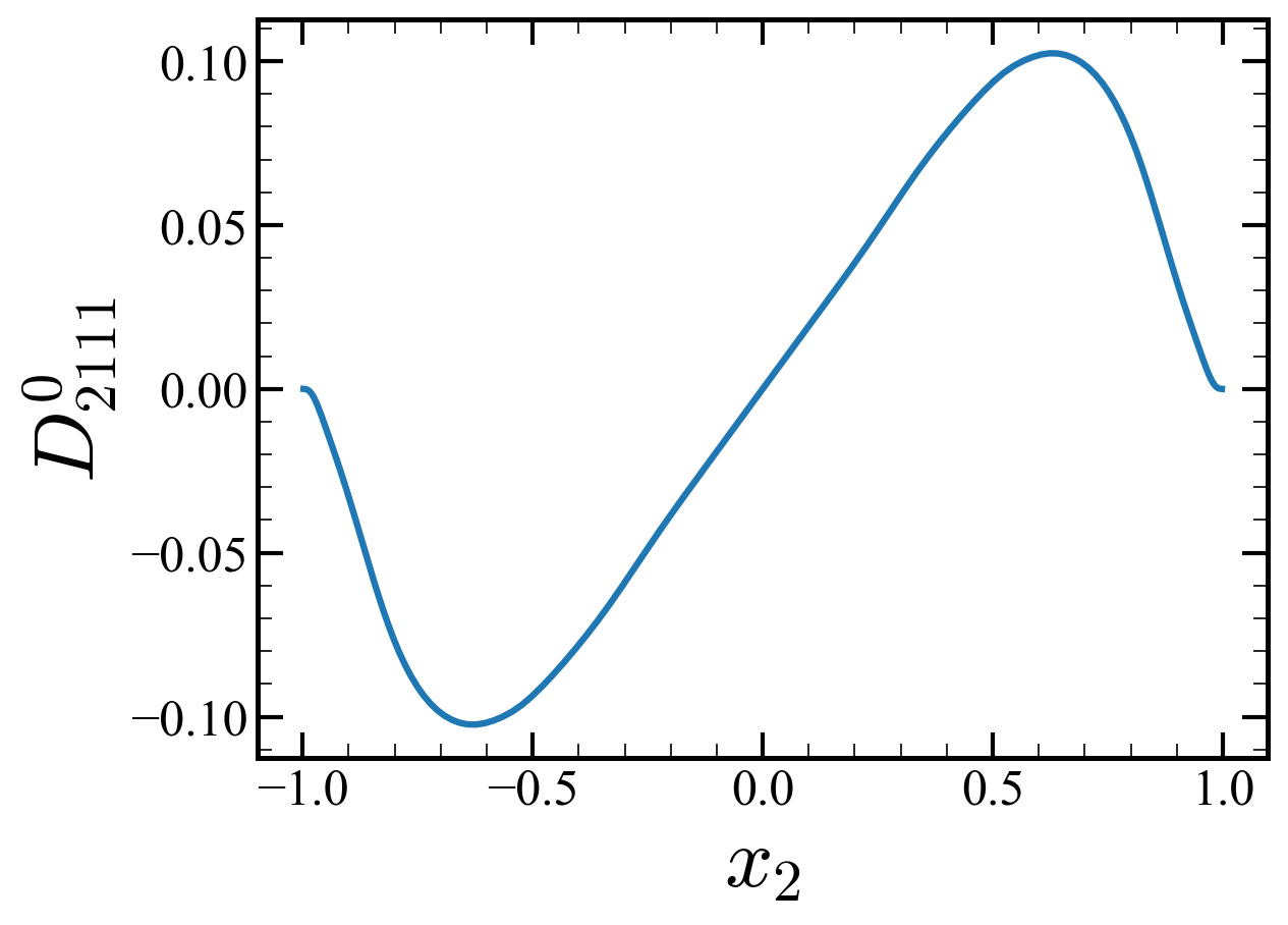
(b) $D_{2111}$

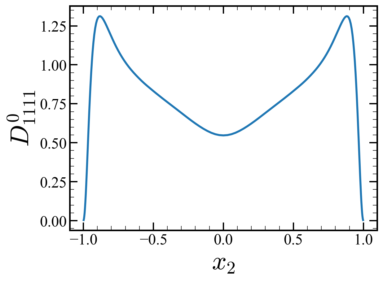
(c) $D_{1111}$

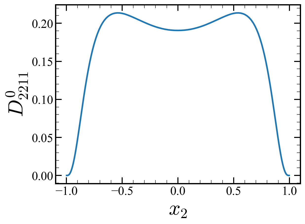
(d) $D_{2211}$

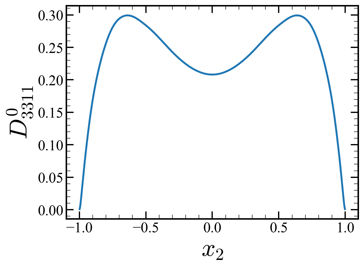
(e) $D_{3311}$

Figure 16: Distribution of nonzero $D^{0}_{ij11}$.

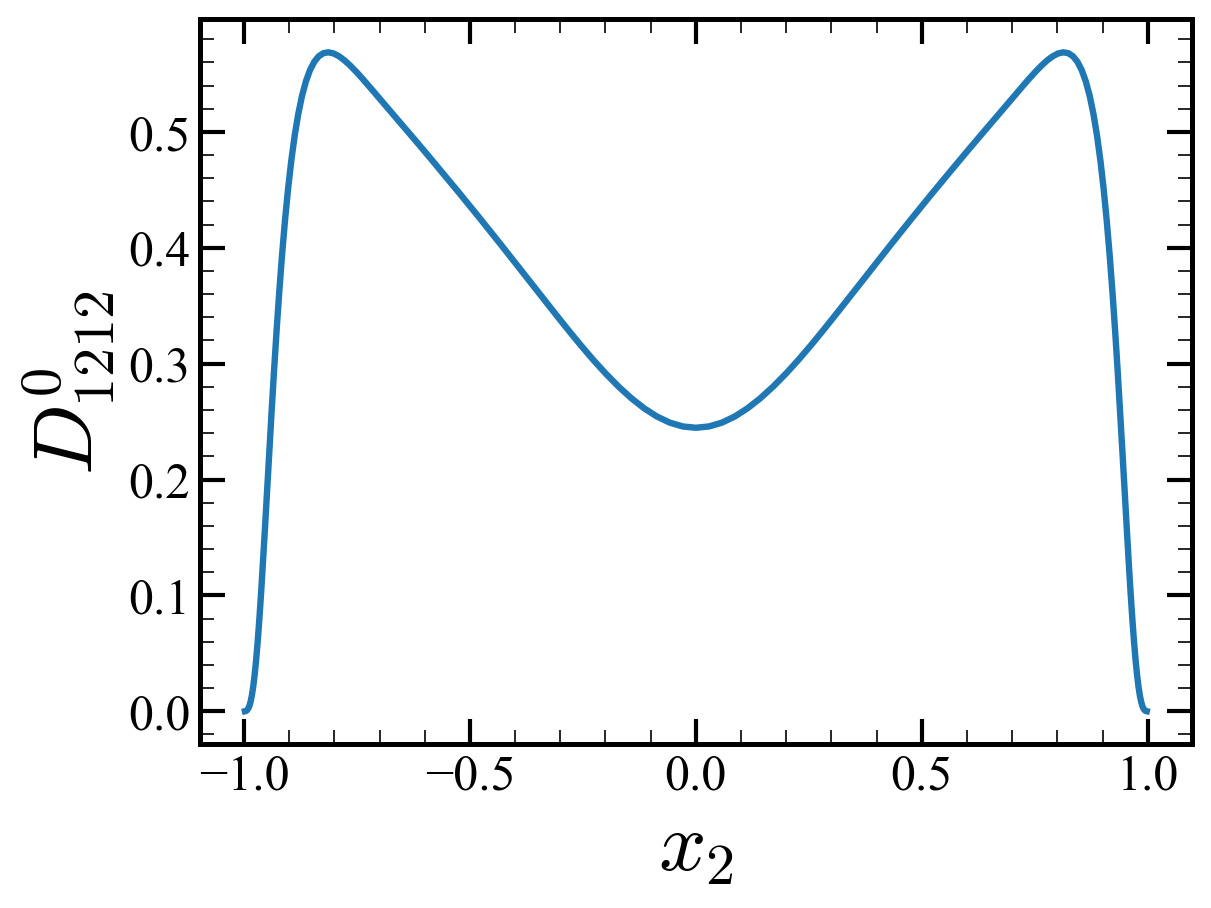
(a) $D_{1212}$

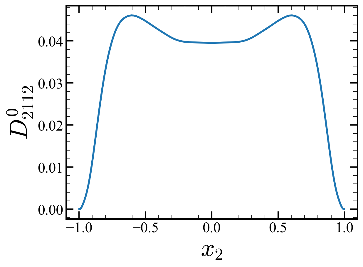
(b) $D_{2112}$

(c) $D_{1112}$

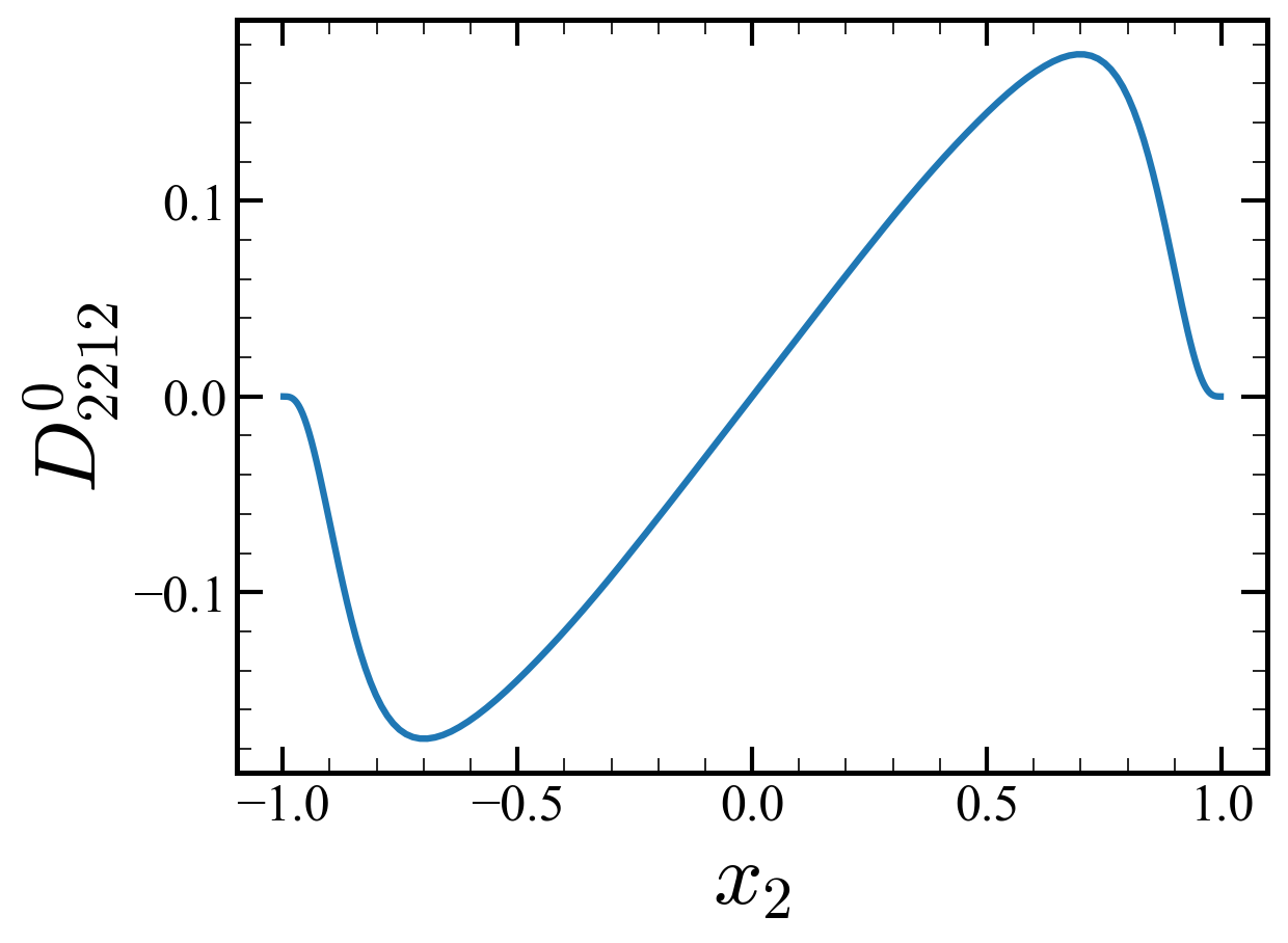
(d) $D_{2212}$

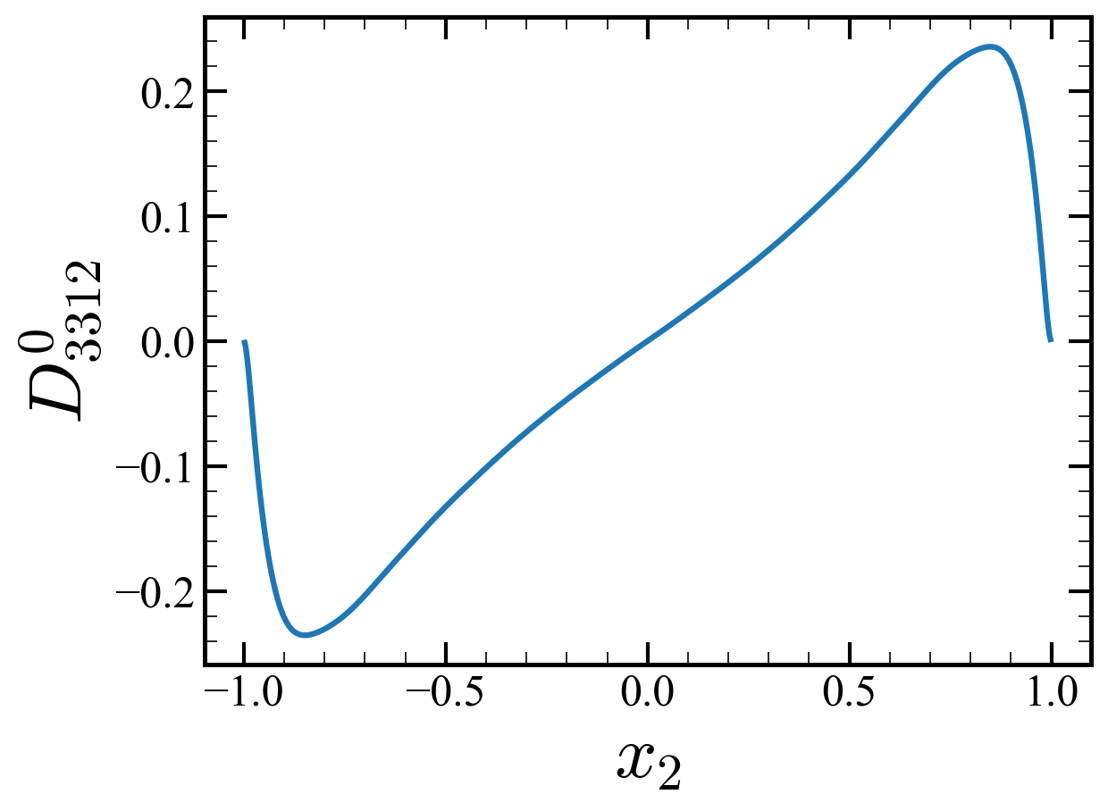
(e) $D_{3312}$

Figure 17: Distribution of nonzero $D^{0}_{ij12}$.

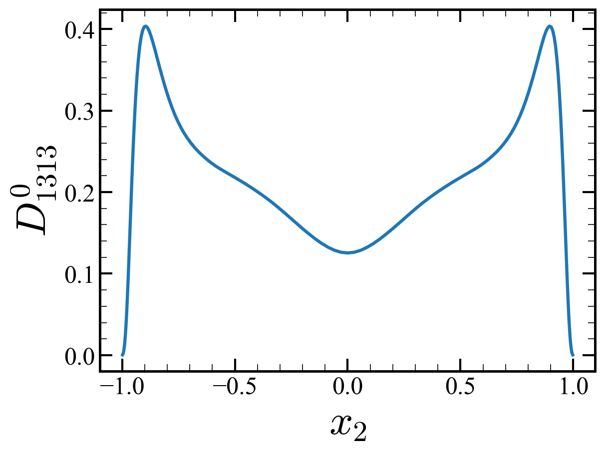
(a) $D_{1313}$

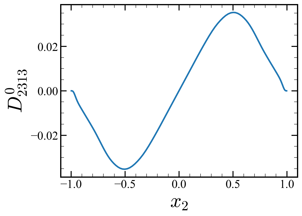
(b) $D_{2313}$

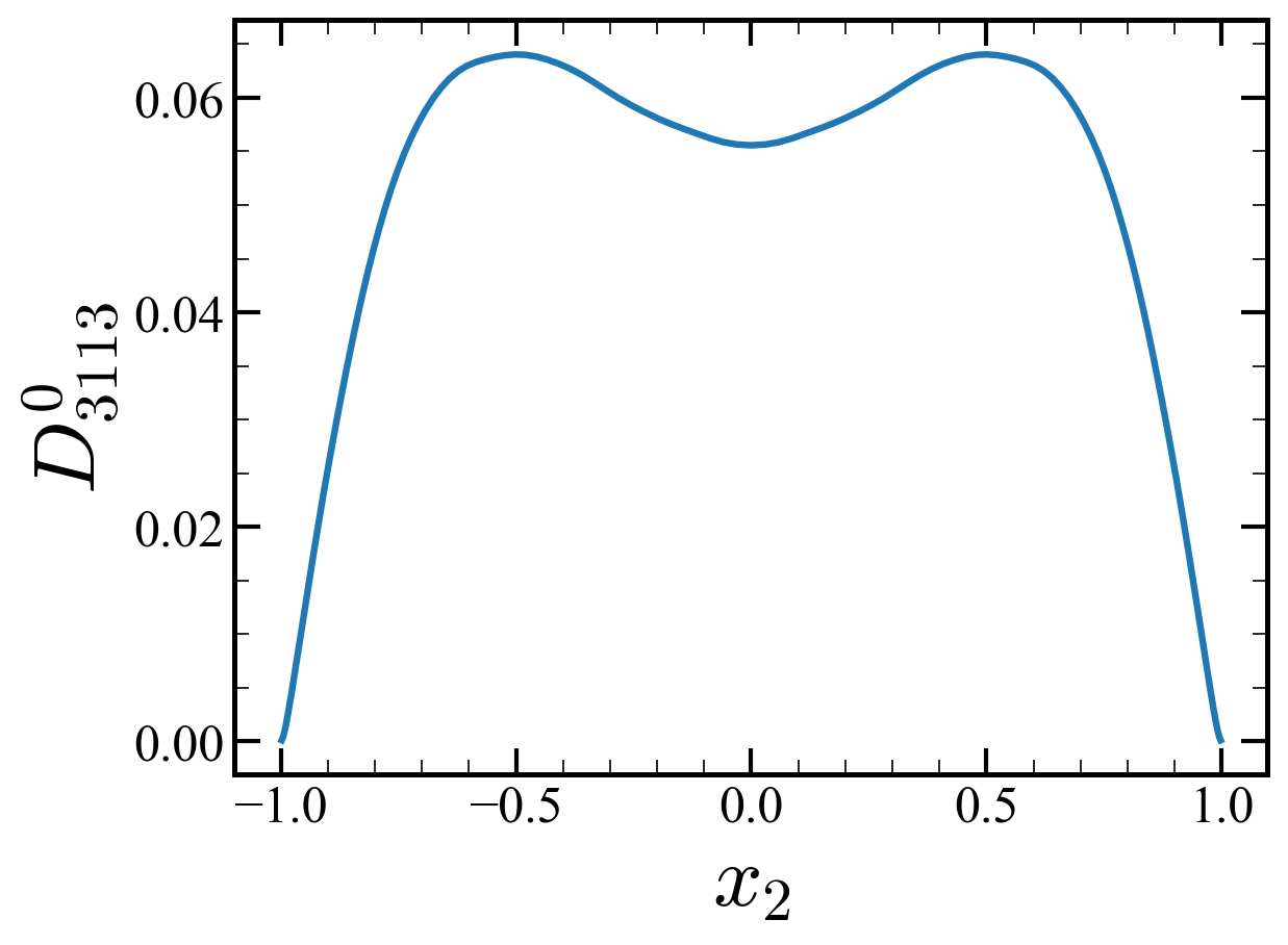
(c) $D_{3113}$

(d) $D_{3213}$

Figure 18: Distribution of nonzero $D^{0}_{ij13}$.

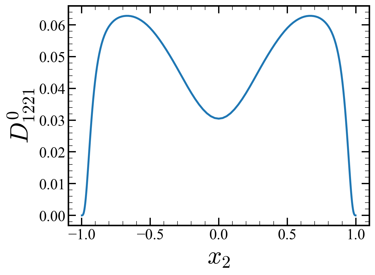
(a) $D_{1221}$

(b) $D_{2121}$

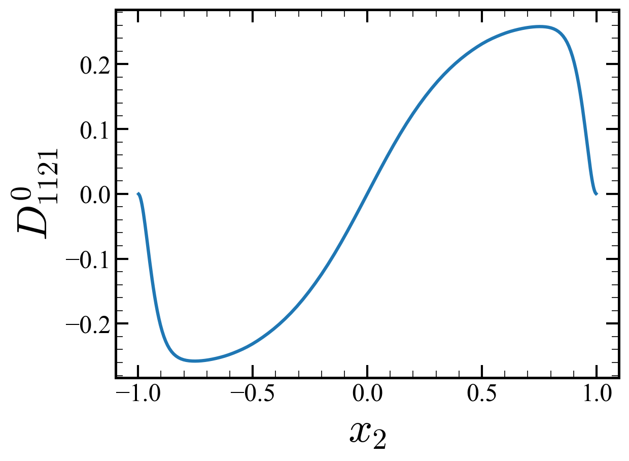
(c) $D_{1121}$

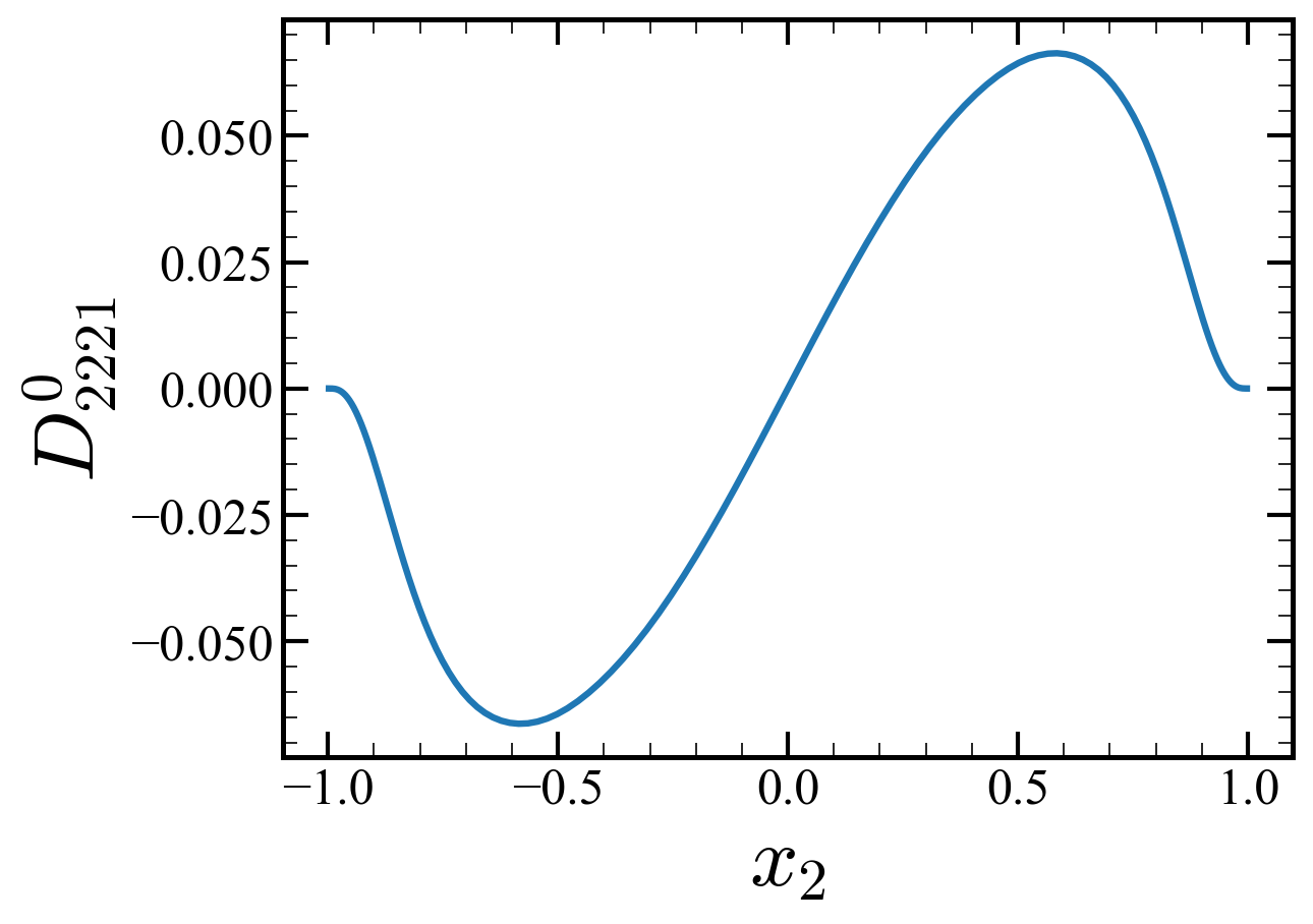
(d) $D_{2221}$

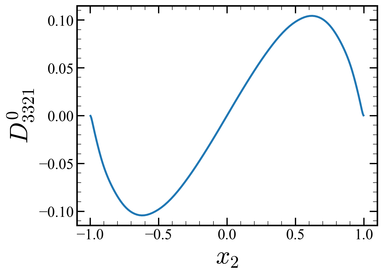
(e) $D_{3321}$

Figure 19: Distribution of nonzero $D^{0}_{ij21}$.

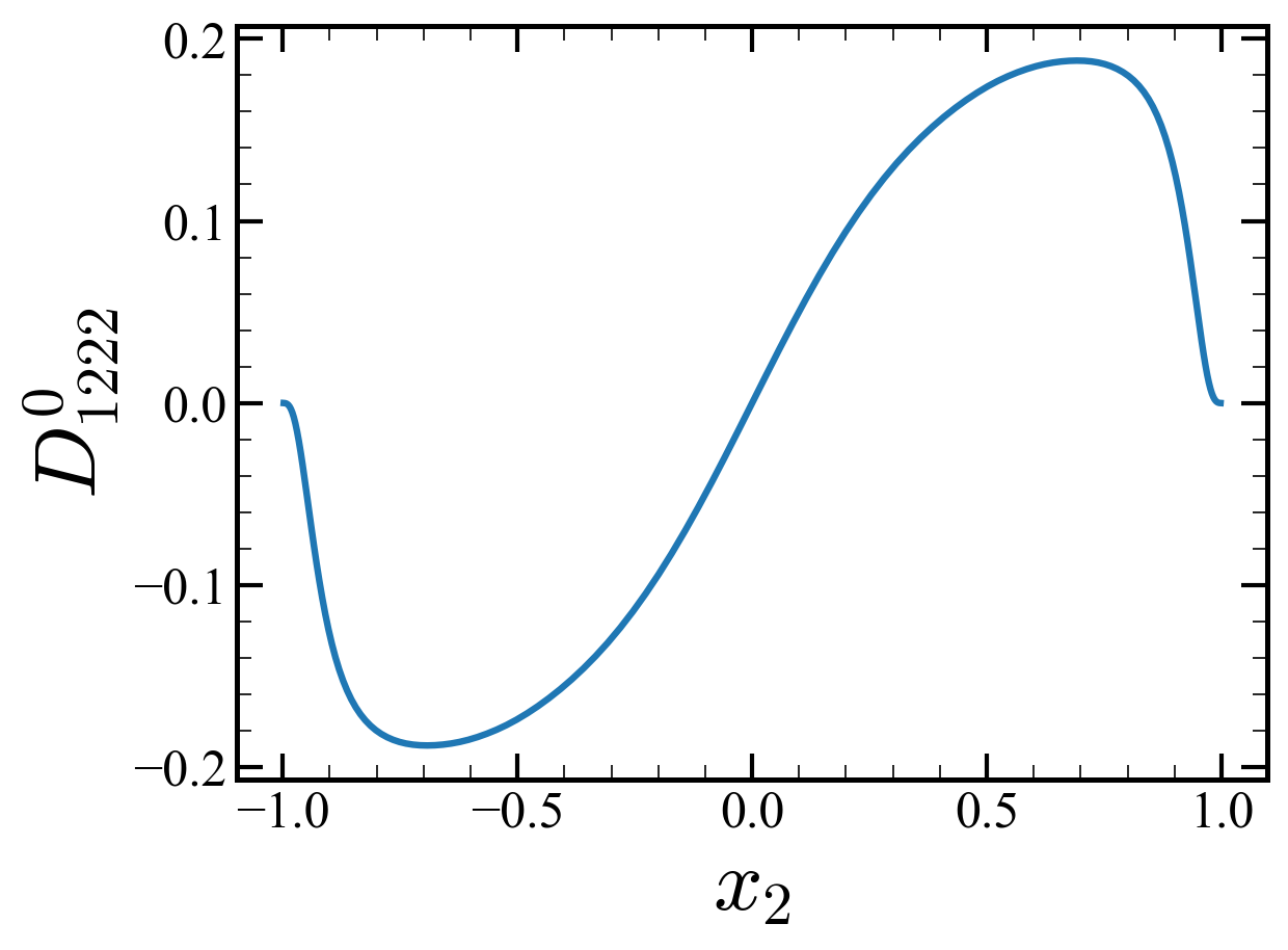
(a) $D_{1222}$

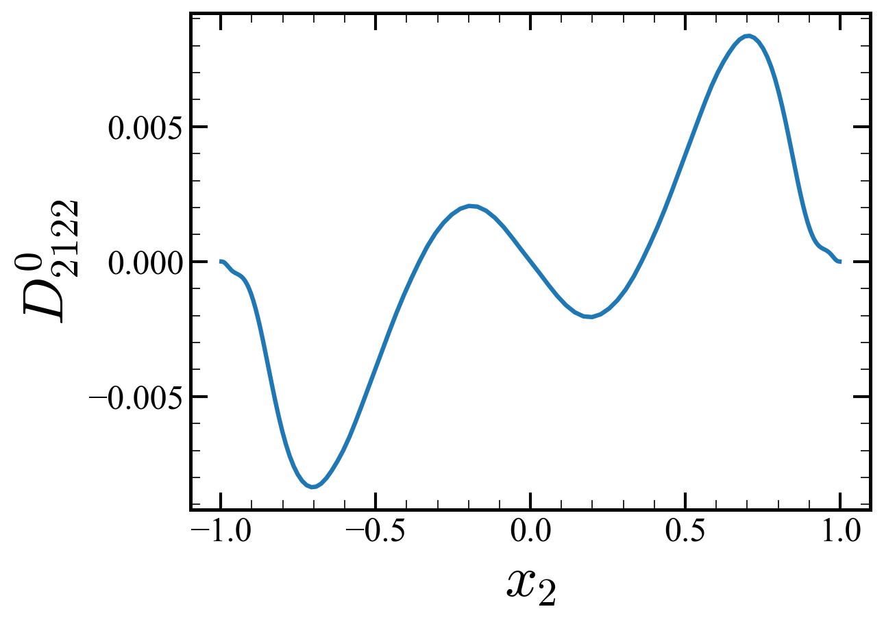
(b) $D_{2122}$

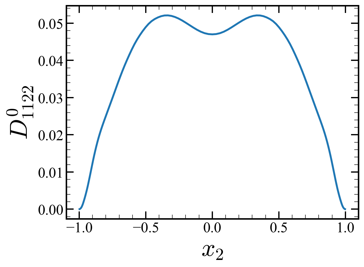
(c) $D_{1122}$

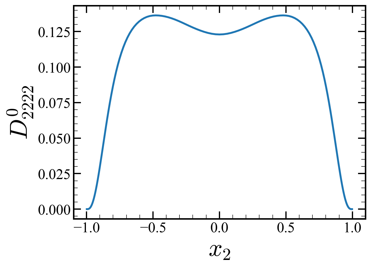
(d) $D_{2222}$

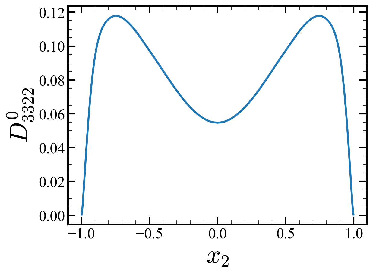
(e) $D_{3322}$

Figure 20: Distribution of nonzero $D^{0}_{ij22}$.

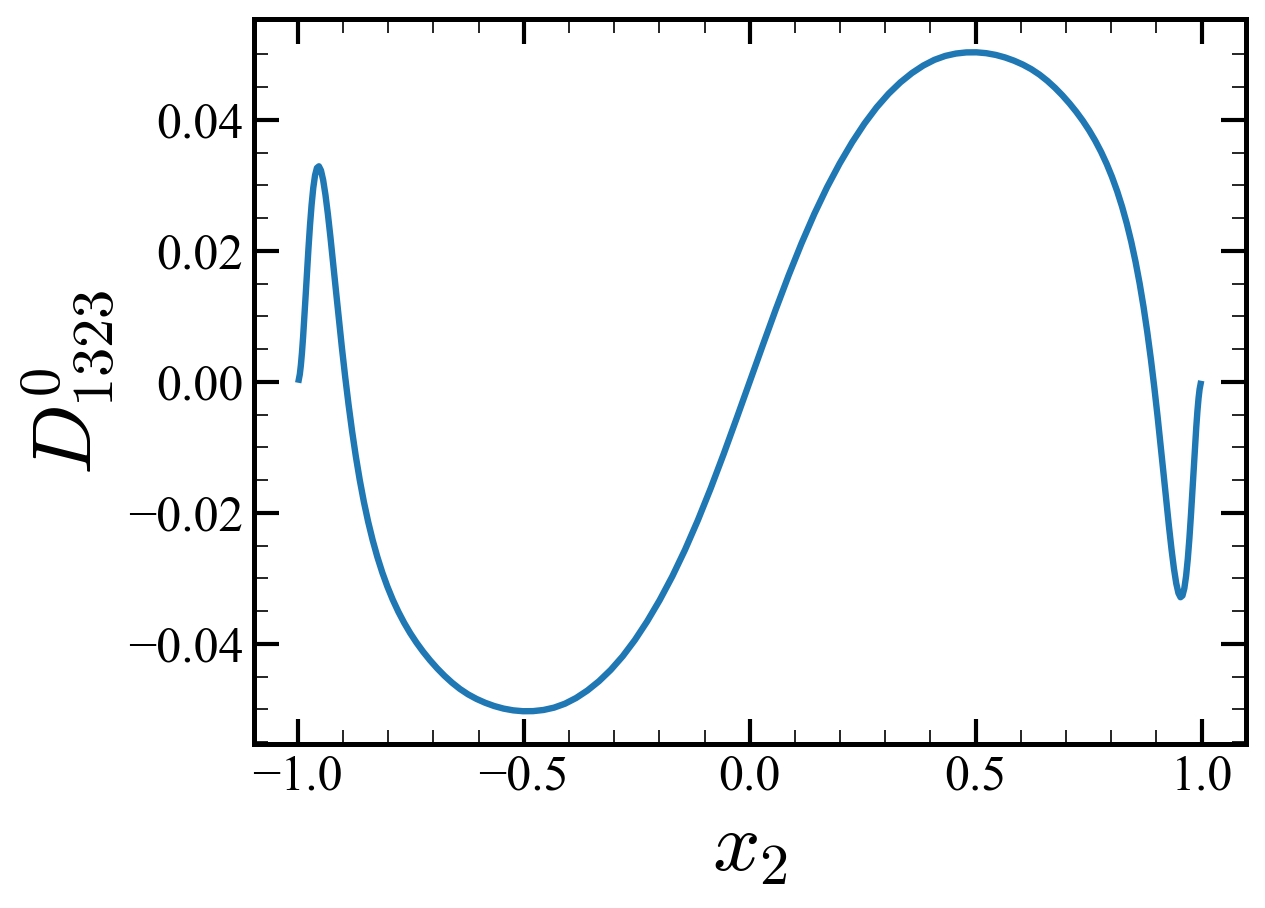
(a) $D_{1323}$

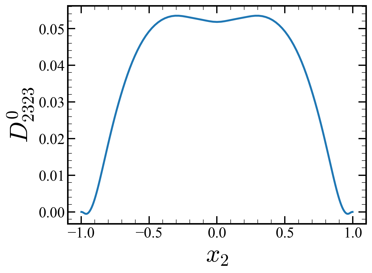
(b) $D_{2323}$

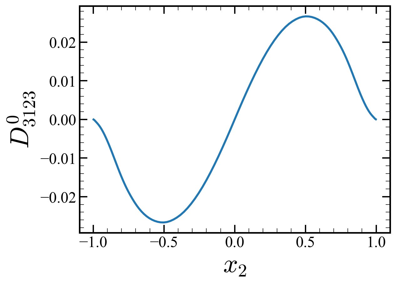
(c) $D_{3123}$

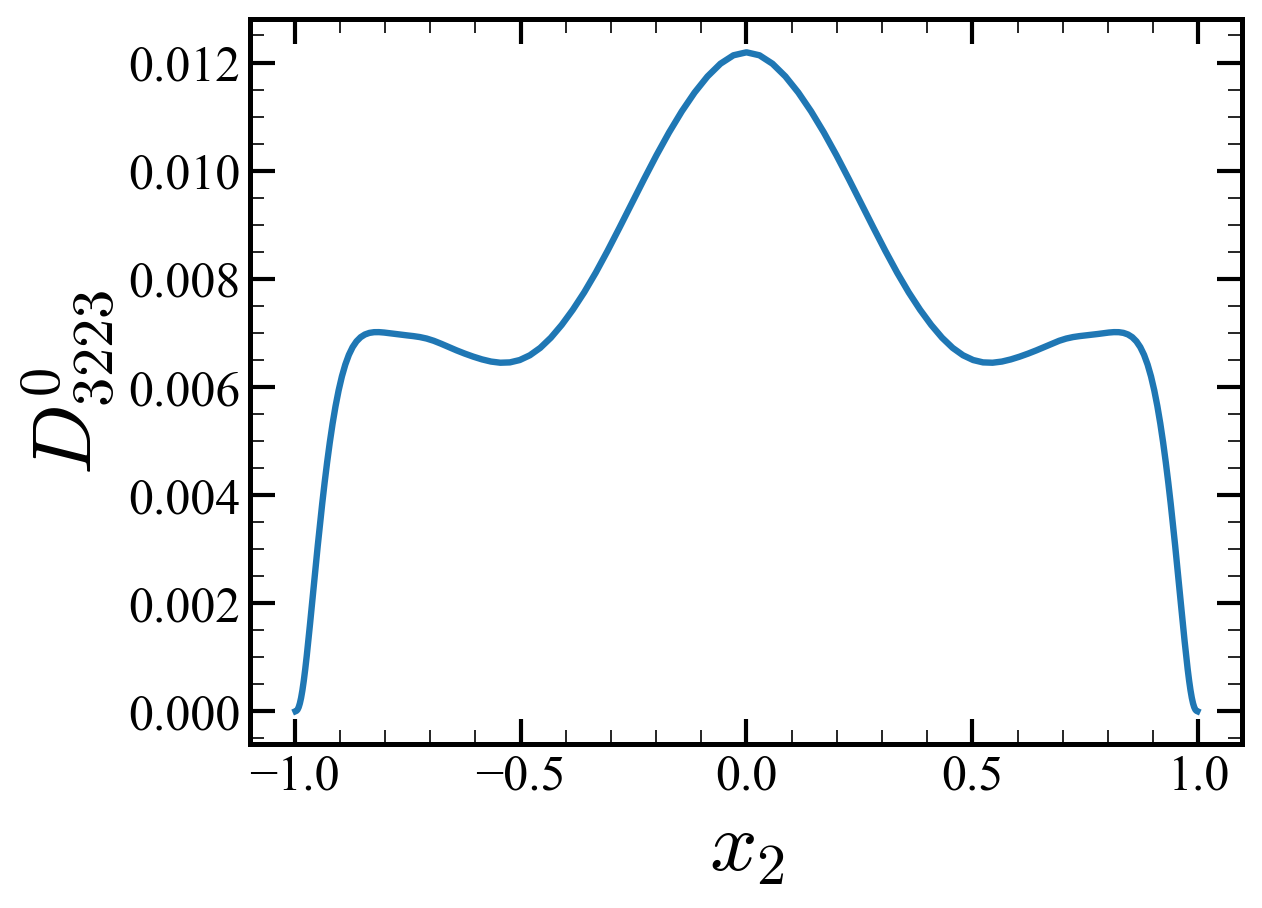
(d) $D_{3223}$

Figure 21: Distribution of nonzero $D^{0}_{ij23}$.

(a) $D_{1331}$

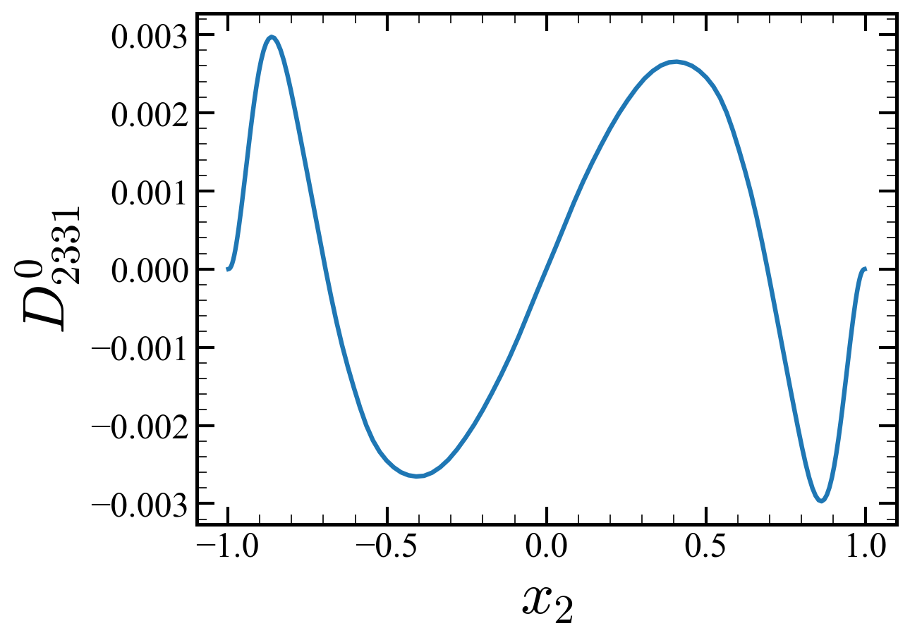
(b) $D_{2331}$

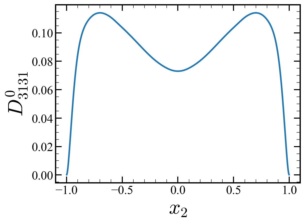
(c) $D_{3131}$

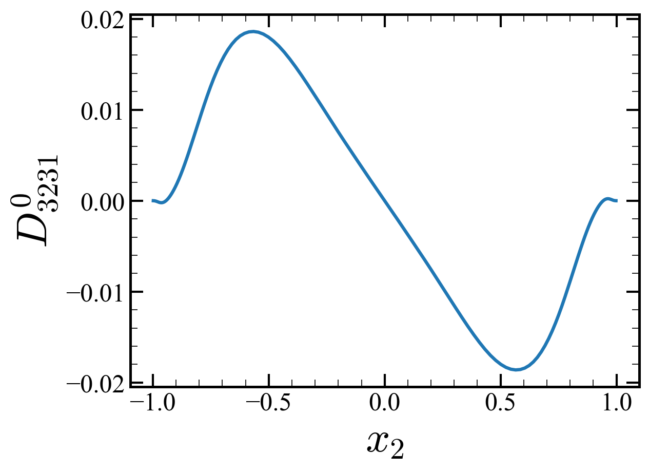
(d) $D_{3231}$

Figure 22: Distribution of nonzero $D^{0}_{ij31}$.

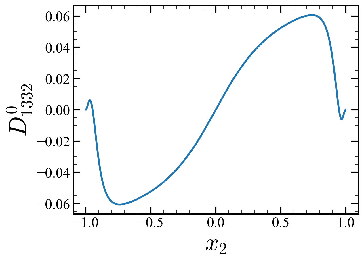
(a) $D_{1332}$

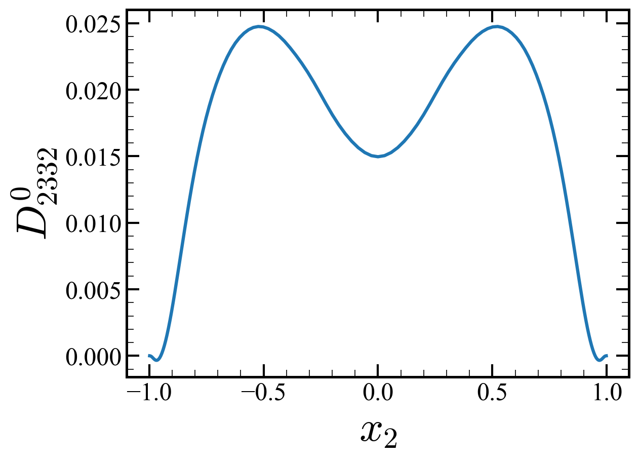
(b) $D_{2332}$

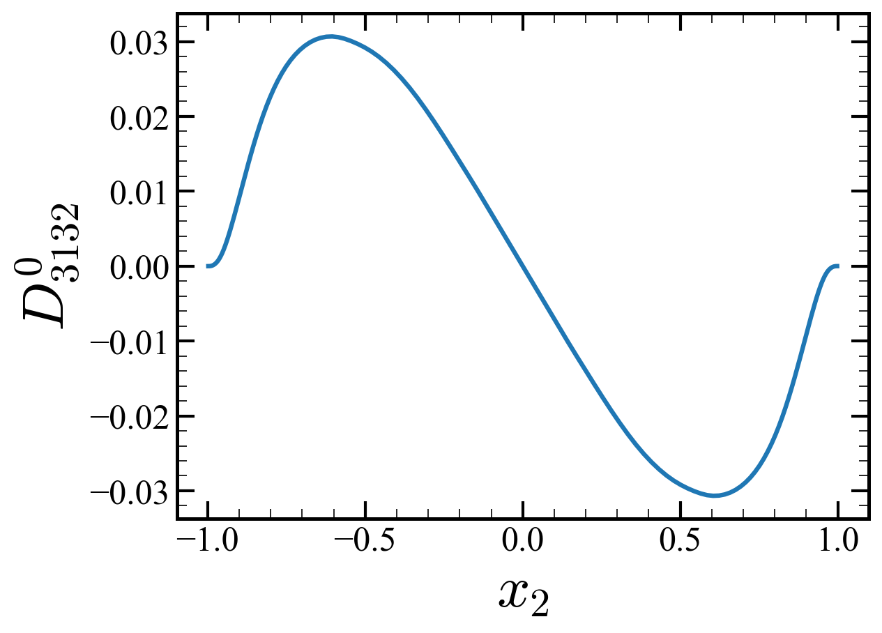
(c) $D_{3132}$

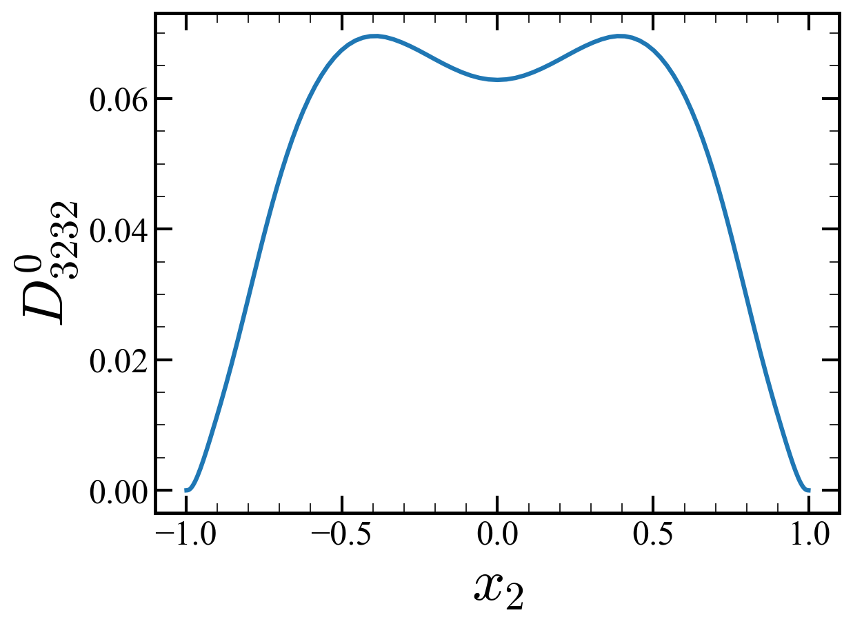
(d) $D_{3232}$

Figure 23: Distribution of nonzero $D^{0}_{ij32}$.

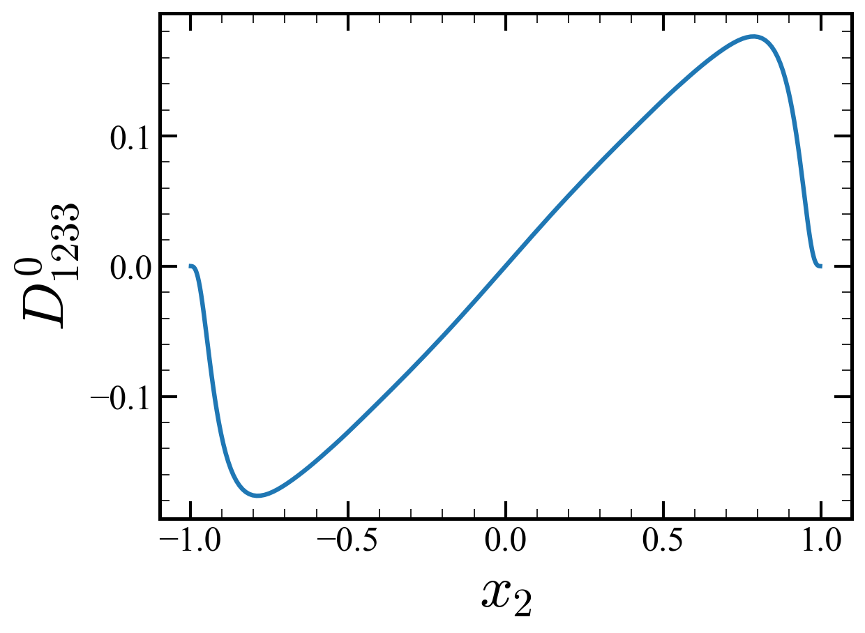
(a) $D_{1233}$

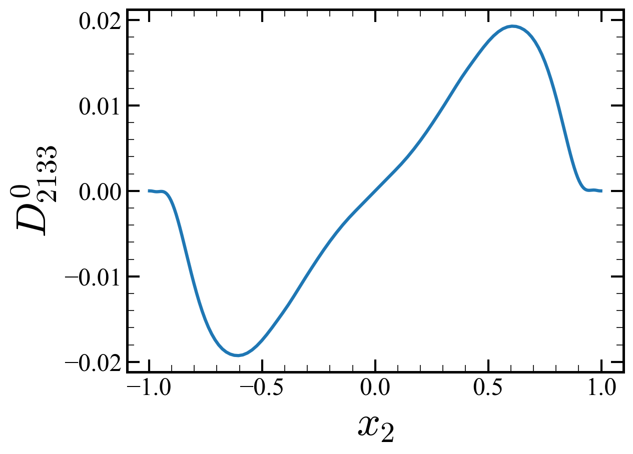
(b) $D_{2133}$

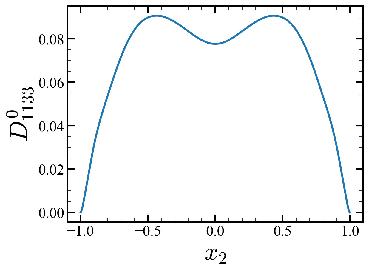
(c) $D_{1133}$

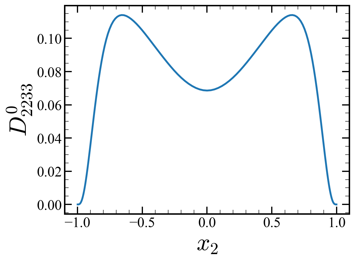
(d) $D_{2233}$

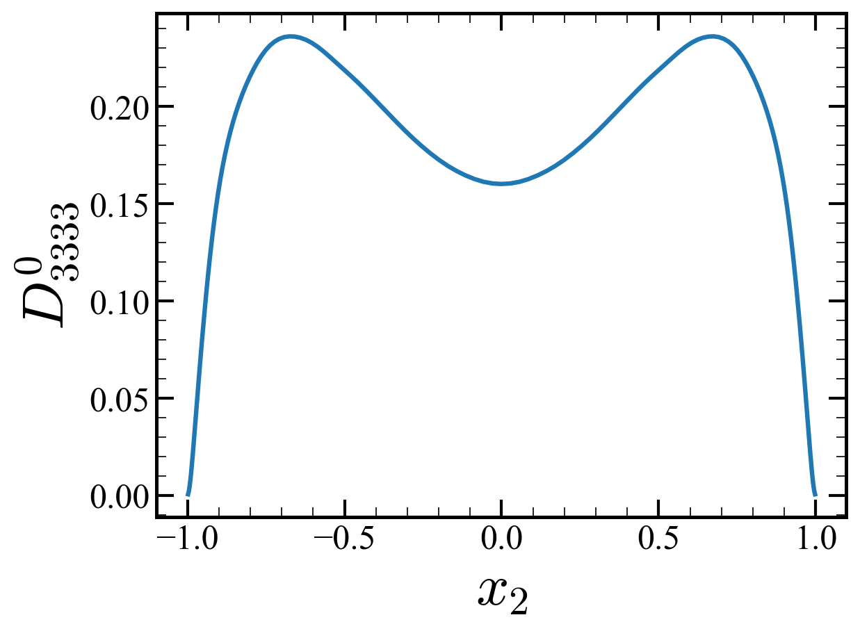
(e) $D_{3333}$

Figure 24: Distribution of nonzero $D^{0}_{ij33}$.

This appendix provides the entire nonzero values of the leading-order eddy viscosity tensor $D^{0}_{ijkl}$ (Figure 16-24). This corresponds to the eddy viscosity tensor in Equation 12. The values not shown converge to zero.

Appendix D Scaling analysis for 2D spatially developing boundary layer

To determine which components of the eddy viscosity tensor are critical to the RANS of the two-dimensional spatially developing boundary layer, we conduct the following scaling analysis. The flow system with the streamwise length scale $l$ and the wall-normal length scale $d$ is considered where $l\gg d$. Based on the correlation by White & Majdalani (2006), a typical ratio for $\mathrm{Re}_{x}\sim O(10^{6})$ is $d/l\sim 0.02$. Using the leading-order eddy viscosity tensor model, Equation 12, the Reynolds stress term includes a summation of the eddy viscosity tensor terms. For instance, $\overline{u_{2}^{\prime}u_{1}^{\prime}}$ is represented as follows:

$$-\overline{u_{2}^{\prime}u_{1}^{\prime}}=D_{2111}\frac{\partial U_{1}}{\partial x_{1}}+D_{2112}\frac{\partial U_{2}}{\partial x_{1}}+D_{2121}\frac{\partial U_{1}}{\partial x_{2}}+D_{2122}\frac{\partial U_{2}}{\partial x_{2}}$$ (22)

One needs to consider not only the magnitude of the eddy viscosity tensor element but also the estimated scales of each term in this equation. To evaluate the length scales for the velocity, we set $U_{1}\sim 1$, and the continuity enforces $U_{2}\sim d/l$. Ignoring $D_{21kl}$ coefficients, the length scales of the four terms on the right-hand side are $1/l$, $d/{l^{2}}$, $1/d$, and $1/l$. Since $l\gg d$, $D_{2121}$ plays the major role for this Reynolds stress. The next two are the terms that multiply $D_{2111}$ and $D_{2122}$. However, MFM reveals that $D_{2111}$ is one order of magnitude larger than $D_{2122}$. Hence, $D_{2111}$ is the next important eddy viscosity tensor for this Reynolds stress. Likewise, we conducted scaling analysis for all other Reynolds stresses. The analysis informs that $D_{1111}$, $D_{1121}$, $D_{2121}$, and $D_{2221}$ are among the most significant eddy viscosity tensor elements for the case of slowly developing semi-parallel wall-bounded flows.

Appendix E MFM for $D_{ij21}$ measurement

To compute the eddy viscosity kernel $D_{ij21}\left(x_{2},y_{2}\right)$, we use brute force MFM method using delta function forcing of the velocity gradient at each location. We start from the full kernel eddy viscosity representation in Equation 8. We macroscopically force the mean velocity gradient by ${\partial V_{l}}/{\partial x_{k}}=\delta\left(y_{2}-y_{2}^{*}\right)\delta_{k2}\delta_{l1}$, where $\delta(x)$ represents Dirac delta function, $\delta_{ij}$ represents Kronecker delta in index notation, and $y_{2}^{*}$ is the probing location of the eddy viscosity. With such forcing, Equation 8 becomes the following:

$$-\overline{u_{i}^{\prime}v_{j}^{\prime}}(x_{2}) =\int D_{ijkl}\left({x_{2}},{y_{2}}\right)\left.\frac{\partial V_{l}}{\partial x_{k}}\right|_{{y_{2}}}\mathrm{d}y_{2}$$

$$=\int D_{ijkl}\left({x_{2}},{y_{2}}\right)\delta\left(y_{2}-y_{2}^{*}\right)\delta_{k2}\delta_{l1}\mathrm{d}y_{2}$$

$$=D_{ij21}\left(x_{2},y_{2}=y_{2}^{*}\right)$$

Forcing that would maintain the mean streamwise velocity as a Dirac delta function at $y_{2}=y_{2}^{*}$ reveals the eddy viscosity kernel $D_{ij21}\left(x_{2},y_{2}=y_{2}^{*}\right)$. By setting $y_{2}^{*}$ for all possible locations, we can obtain the eddy viscosity kernel $D_{ij21}$. In numerical implementation of this strategy, instead of dealing with Dirac delta functions, we selected $V_{1}$ to be a step function with respect to the $y_{2}$ direction. In discrete space, the MFM is conducted at each discrete point of $y_{2}^{*}$ in wall-normal direction with a corresponding heaviside function where the discontinuous point lies at that point. In order to compute the entire kernel $D_{ij21}$, one need to conduct many MFM simulations. More specifically, the number of simulations has to be the number of degree of freedom of the Reynolds-averaged space, i.e. the number of mesh points in the wall-normal direction. For instance, since our RANS space has 144 cell centers, we need 146 MFM simulations, including two for the boundary values.

References

- Batchelor (1949) Batchelor, G. 1949 Diffusion in a field of homogeneous turbulence. i. eulerian analysis. Australian Journal of Chemistry 2 (4), 437–450.
- Bose et al. (2010) Bose, S. T., Moin, P. & You, D. 2010 Grid-independent large-eddy simulation using explicit filtering. Physics of Fluids 22 (10).
- Boussinesq (1877) Boussinesq, J. 1877 Essai sur la théorie des eaux courantes. Impr. nationale.
- Cécora et al. (2015) Cécora, R.-D., Radespiel, R., Eisfeld, B. & Probst, A. 2015 Differential reynolds-stress modeling for aeronautics. AIAA Journal 53 (3), 739–755.
- Champagne et al. (1970) Champagne, F., Harris, V. & Corrsin, S. 1970 Experiments on nearly homogeneous turbulent shear flow. Journal of Fluid Mechanics 41 (1), 81–139.
- Chien (1982) Chien, K.-Y. 1982 Predictions of channel and boundary-layer flows with a low-reynolds-number turbulence model. AIAA journal 20 (1), 33–38.
- Cimarelli et al. (2019) Cimarelli, A., Leonforte, A., De Angelis, E., Crivellini, A. & Angeli, D. 2019 On negative turbulence production phenomena in the shear layer of separating and reattaching flows. Physics Letters A 383 (10), 1019–1026.
- Coleman et al. (1996) Coleman, G. N., Kim, J. & Le, A.-T. 1996 A numerical study of three-dimensional wall-bounded flows. International journal of heat and fluid flow 17 (3), 333–342.
- Du Vachat (1977) Du Vachat, R. 1977 Realizability inequalities in turbulent flows. Physics of Fluids 20 (4), 551–556.
- Durbin (1993) Durbin, P. 1993 A reynolds stress model for near-wall turbulence. Journal of Fluid Mechanics 249, 465–498.
- Eitel-Amor et al. (2015) Eitel-Amor, G., Örlü, R., Schlatter, P. & Flores, O. 2015 Hairpin vortices in turbulent boundary layers. Physics of Fluids 27 (2).
- Gerolymos et al. (2012) Gerolymos, G., Lo, C., Vallet, I. & Younis, B. 2012 Term-by-term analysis of near-wall second-moment closures. AIAA journal 50 (12), 2848–2864.
- Hamba (2005) Hamba, F. 2005 Nonlocal analysis of the reynolds stress in turbulent shear flow. Physics of Fluids 17 (11).
- Hamba (2013) Hamba, F. 2013 Exact transport equation for local eddy viscosity in turbulent shear flow. Physics of Fluids 25 (8).
- Hanjalić & Launder (1972) Hanjalić, K. & Launder, B. E. 1972 A reynolds stress model of turbulence and its application to thin shear flows. Journal of Fluid Mechanics 52 (4), 609–638.
- Harris et al. (1977) Harris, V., Graham, J. & Corrsin, S. 1977 Further experiments in nearly homogeneous turbulent shear flow. Journal of Fluid Mechanics 81 (4), 657–687.
- Hinze (1959) Hinze, J. 1959 Turbulence: An introduction to its mechanism and theory. McGraw-Hill Book Company, Inc p. 22.
- Kim & Moin (1985) Kim, J. & Moin, P. 1985 Application of a fractional-step method to incompressible navier-stokes equations. Journal of Computational Physics 59 (2), 308–323.
- Kraichnan (1987) Kraichnan, R. H. 1987 Eddy viscosity and diffusivity: exact formulas and approximations. Complex Systems 1 (4-6), 805–820.
- Launder et al. (1975) Launder, B. E., Reece, G. J. & Rodi, W. 1975 Progress in the development of a reynolds-stress turbulence closure. Journal of Fluid Mechanics 68 (3), 537–566.
- Liu et al. (2021) Liu, J., Williams, H. & Mani, A. 2021 A systematic approach for obtaining and modeling a nonlocal eddy diffusivity. arXiv preprint arXiv:2111.03914 .
- Mani & Park (2021) Mani, A. & Park, D. 2021 Macroscopic forcing method: A tool for turbulence modeling and analysis of closures. Physical Review Fluids 6 (5), 054607.
- Mani et al. (2013) Mani, M., Babcock, D., Winkler, C. & Spalart, P. 2013 Predictions of a supersonic turbulent flow in a square duct. In 51st AIAA Aerospace Sciences Meeting Including the New Horizons Forum and Aerospace Exposition, p. 860.
- Menter (1994) Menter, F. R. 1994 Two-equation eddy-viscosity turbulence models for engineering applications. AIAA Journal 32 (8), 1598–1605.
- Milani (2020) Milani, P. M. 2020 Machine learning approaches to model turbulent mixing in film cooling flows. PhD thesis.
- Moin & Kim (1982) Moin, P. & Kim, J. 1982 Numerical investigation of turbulent channel flow. Journal of Fluid Mechanics 118, 341–377.
- Morinishi et al. (1998) Morinishi, Y., Lund, T. S., Vasilyev, O. V. & Moin, P. 1998 Fully conservative higher order finite difference schemes for incompressible flow. Journal of Computational Physics 143 (1), 90–124.
- Pope (2001) Pope, S. B. 2001 Turbulent flows.
- Rogallo (1981) Rogallo, R. S. 1981 Numerical experiments in homogeneous turbulence 81315.
- Rogers et al. (1989) Rogers, M. M., Mansour, N. N. & Reynolds, W. C. 1989 An algebraic model for the turbulent flux of a passive scalar. Journal of Fluid Mechanics 203, 77–101.
- Rogers & Moin (1987) Rogers, M. M. & Moin, P. 1987 The structure of the vorticity field in homogeneous turbulent flows. Journal of Fluid Mechanics 176, 33–66.
- Rumsey et al. (2020) Rumsey, C., Carlson, J.-R., Pulliam, T. & Spalart, P. 2020 Improvements to the quadratic constitutive relation based on nasa juncture flow data. AIAA Journal 58 (10), 4374–4384.
- Schumann (1977) Schumann, U. 1977 Realizability of reynolds-stress turbulence models. Physics of Fluids 20 (5), 721–725.
- Seo et al. (2015) Seo, J., García-Mayoral, R. & Mani, A. 2015 Pressure fluctuations and interfacial robustness in turbulent flows over superhydrophobic surfaces. Journal of Fluid Mechanics 783, 448–473.
- Shirian & Mani (2022) Shirian, Y. & Mani, A. 2022 Eddy diffusivity operator in homogeneous isotropic turbulence. Physical Review Fluids 7 (5), L052601.
- Spalart & Allmaras (1994) Spalart, P. & Allmaras, S. 1994 A one-equation turbulence model for aerodynamic flows. La Recherche Aérospatiale (1), 5–21.
- Spalart (2000) Spalart, P. R. 2000 Strategies for turbulence modelling and simulations. International Journal of Heat and Fluid Flow 21 (3), 252–263.
- Speziale et al. (1994) Speziale, C. G., Abid, R. & Durbin, P. A. 1994 On the realizability of reynolds stress turbulence closures. Journal of Scientific Computing 9, 369–403.
- Speziale et al. (1991) Speziale, C. G., Sarkar, S. & Gatski, T. B. 1991 Modelling the pressure–strain correlation of turbulence: an invariant dynamical systems approach. Journal of Fluid Mechanics 227, 245–272.
- Stanišić & Groves (1965) Stanišić, M. M. & Groves, R. N. 1965 On the eddy viscosity of incompressible turbulent flow. Zeitschrift für angewandte Mathematik und Physik ZAMP 16 (5), 709–712.
- Van Kampen (1992) Van Kampen, N. G. 1992 Stochastic processes in physics and chemistry, , vol. 1. Elsevier.
- Warhaft (1980) Warhaft, Z. 1980 An experimental study of the effect of uniform strain on thermal fluctuations in grid-generated turbulence. Journal of Fluid Mechanics 99 (3), 545–573.
- White & Majdalani (2006) White, F. M. & Majdalani, J. 2006 Viscous fluid flow, , vol. 3. McGraw-Hill New York.
- Wilcox (2008) Wilcox, D. C. 2008 Formulation of the kw turbulence model revisited. AIAA journal 46 (11), 2823–2838.
- Wilcox et al. (1998) Wilcox, D. C. & others 1998 Turbulence modeling for CFD, , vol. 2. DCW industries La Canada, CA.