The Most Metal-poor Stars in the Magellanic Clouds are $r$-process Enhanced

Abstract

The chemical abundances of a galaxy’s metal-poor stellar population can be used to investigate the earliest stages of its formation and chemical evolution. The Magellanic Clouds are the most massive of the Milky Way’s satellite galaxies and are thought to have evolved in isolation until their recent accretion by the Milky Way. Unlike the Milky Way’s less massive satellites, little is know about the Magellanic Clouds’ metal-poor stars. We have used the mid-infrared metal-poor star selection of Schlaufman & Casey (2014) and archival data to target nine LMC and four SMC giants for high-resolution Magellan/MIKE spectroscopy. These nine LMC giants with $-2.4\lesssim[\text{Fe/H}]\lesssim-1.5$ and four SMC giants with $-2.6\lesssim[\text{Fe/H}]\lesssim-2.0$ are the most metal-poor stars in the Magellanic Clouds yet subject to a comprehensive abundance analysis. While we find that at constant metallicity these stars are similar to Milky Way stars in their $\alpha$, light, and iron-peak elemental abundances, both the LMC and SMC are enhanced relative to the Milky Way in the $r$-process element europium. These abundance offsets are highly significant, equivalent to$3.9\sigma$ for the LMC, $2.7\sigma$ for the SMC, and $5.0\sigma$ for the complete Magellanic Cloud sample. We propose that the $r$-process enhancement of the Magellanic Clouds’ metal-poor stellar population is a result of the Magellanic Clouds’ isolated chemical evolution and long history of accretion from the cosmic web combined with $r$-process nucleosynthesis on a timescale longer than the core-collapse supernova timescale but shorter than or comparable to the thermonuclear (i.e., Type Ia) supernova timescale.

1 Introduction

A common goal of Local Group galactic archaeology is the use of the elemental abundances of a galaxy’s metal-poor stars to constrain its formation and early chemical evolution (e.g., Beers & Christlieb, 2005; Tolstoy et al., 2009; Frebel & Norris, 2015; Simon, 2019). The formation and early chemical evolution of massive spiral galaxies like the Milky Way and M31 with $M_{\text{tot}}\sim 10^{12}~{}M_{\odot}$ (e.g., Wang et al., 2020; Kafle et al., 2018) resulted from complex interactions between inflows, star formation, stellar evolution, nucleosynthesis, and outflows (e.g., Kobayashi et al., 2006, 2020). In the metallicity range $-3\lesssim[\text{Fe/H}]\lesssim-1$, stars in both the Milky Way and M31 have supersolar abundances relative to iron of titanium and the $\alpha$ elements magnesium, silicon, and calcium (e.g., McWilliam et al., 1995a, b; Escala et al., 2019, 2020a, 2020b; Gilbert et al., 2020). The supersolar $[\alpha/\text{Fe}]$ abundance ratios observed in these stars are thought to result from nucleosynthesis in core-collapse supernovae that start enriching a galaxy’s interstellar medium just a few Myr after the onset of star formation (e.g, Woosley & Weaver, 1995; Heger & Woosley, 2010; Sukhbold et al., 2016). The eventual prolific nucleosynthesis of iron-peak elements in thermonuclear (i.e., Type Ia) supernovae starting a few tens to 100 Myr after the onset of star formation causes the $[\alpha/\text{Fe}]$ abundance ratio to approach solar as $[\text{Fe/H}]$ approaches zero (e.g., Maoz et al., 2014). The $[\text{Fe/H}]$ value at which $[\alpha/\text{Fe}]$ begins to decline (sometimes called the “knee”) therefore corresponds to a point in time a few tens to 100 Myr after the onset of star formation in a stellar population (e.g., Tinsley, 1979). The implication is that both the Milky Way and M31 transitioned from forming stars with $[\text{Fe/H}]\sim-3$ to forming stars with $[\text{Fe/H}]\sim-1$ in less than about 100 Myr. The Milky Way and M31’s high masses and star formation rates necessary to drive chemical evolution from $[\text{Fe/H}]\sim-3$ to $[\text{Fe/H}]\sim-1$ in less than 100 Myr suggest that even rare classes of supernovae should contribute to their chemical evolution.

1.1 Metal-poor Star Formation in Classical and Ultra-faint Dwarf Spheriodal Satellites

The formation and chemical evolution of the Milky Way’s satellite classical and ultra-faint dwarf spheroidal (dSph) galaxies with masses enclosed inside their half-light radii $M_{1/2}$ in the range $10^{5}~{}M_{\odot}\lesssim M_{1/2}\lesssim 10^{8}~{}M_{\odot}$ appear to have been simpler. The Milky Way’s classical dSph galaxies with $10^{7}~{}M_{\odot}\lesssim M_{1/2}\lesssim 10^{8}~{}M_{\odot}$ have extended star formation histories, broad metallicity distributions, and no discernible downturns in $[\alpha/\text{Fe}]$ with increasing $[\text{Fe/H}]$ in the range $-3\lesssim[\text{Fe/H}]\lesssim-1$ (e.g., Tolstoy et al., 2009; Kirby et al., 2011a, b). While simple chemical evolution models are unable to explain all of their observed properties, significant inflows of unenriched gas are usually necessary. Moreover, the importance of unenriched gas inflow relative to gas outflows appears to increase with galaxy luminosity.

Like the Milky Way’s more massive classical dSph galaxies, its ultra-faint dSph galaxies with $10^{5}~{}M_{\odot}\lesssim M_{1/2}\lesssim 10^{7}~{}M_{\odot}$ have extended star formation histories and broad metallicity distributions (e.g., Brown et al., 2012, 2014; Vargas et al., 2013; Weisz et al., 2014). In contrast to their more massive counterparts, the Milky Way’s ultra-faint dSph galaxies stopped forming stars after only a few Gyr. When considered as a population, stars in the Milky Way’s ultra-faint dSph galaxies show a decline in $[\alpha/\text{Fe}]$ with increasing $[\text{Fe/H}]$ in the range $-3\lesssim[\text{Fe/H}]\lesssim-1$ as expected if star formation persisted for more than about 100 Myr and thermonuclear supernovae had an opportunity to contribute to their chemical evolution (e.g., Vargas et al., 2013). Chemical evolution models for ultra-faint dSph galaxies have suggested that they were an order of magnitude less efficient than classical dSph galaxies at turning their cosmological complement of baryons into stars (e.g., Vincenzo et al., 2014). When combined with their low masses, the low star formation efficiencies realized in ultra-faint dSph galaxies indicate that the probability of a rare class of supernova occurring in a single ultra-faint dSph galaxy is small (e.g., Ji et al., 2016a, b).

The formation of metal-poor stars with $[\text{Fe/H}]\lesssim-2$ will persist while a galaxy’s star formation rate is small compared to the inflow rate of unenriched gas from the cosmic web. Alternatively, a galaxy will cease forming metal-poor stars when its star formation rate is large relative to the inflow rate of unenriched gas from the cosmic web. The interplay between star formation and the accretion of unenriched gas is therefore the key determinant of the duration of metal-poor star formation. The available data described above suggests that the chemical evolution of the Milky Way and M31 advanced rapidly through the range $-3\lesssim[\text{Fe/H}]\lesssim-1$. In contrast, the chemical evolution of the Milky Way’s classical and ultra-faint dSph galaxies moved slowly through the range $-3\lesssim[\text{Fe/H}]\lesssim-1$. While the physical processes that halted the inflow of unenriched gas from the cosmic web and therefore ended the era of metal-poor star formation are not directly observable, it is possible to directly study the quenching of metal-rich star formation in nearby galaxies.

1.2 Quenching Metal-poor Star Formation

Galaxies can be roughly categorized using their morphologies and rest-frame optical colors into two classes: spiral or irregular galaxies that are part of a “blue cloud” and elliptical galaxies that are part of a “red sequence” (e.g., Strateva et al., 2001; Blanton et al., 2003; Baldry et al., 2004; Wuyts et al., 2011; van der Wel et al., 2014). While both morphologies and rest-frame optical colors are manifestations of galaxies’ star formation rates, the physical processes responsible for quenching star formation and therefore moving galaxies from the blue cloud to the red sequence are complex and uncertain. It has been shown that both galaxy mass and environment contribute to quenching star formation (e.g., Peng et al., 2010). The implication is that processes both intrinsic and extrinsic to individual galaxies play some role in heating and/or removing cold gas from halos and therefore quenching star formation.

Possible processes responsible for intrinsic quenching are stellar winds & supernovae explosions (e.g., Webster et al., 2014, 2015; Bland-Hawthorn et al., 2015), AGN feedback (e.g., Fabian, 2012), or the shock-heating of cold gas falling onto a galaxy from the cosmic web (e.g., Birnboim & Dekel, 2003; Kereš et al., 2005; Dekel & Birnboim, 2006). The first is expected to be important for lower-mass galaxies with shallower gravitational potentials, while the latter two are expected to be important for massive galaxies with deeper gravitational potentials. Extrinsic quenching of star formation is thought to result from the removal of a galaxy’s cold gas by the reionization of the universe (e.g., Bullock et al., 2000; Somerville, 2002; Benson et al., 2002a, b), ram-pressure stripping (e.g., Gunn & Gott, 1972), or the interdiction of its supply of cold gas in a process called “strangulation” (e.g., Larson et al., 1980; van den Bosch et al., 2008; Putman et al., 2021).

1.3 The Magellanic Clouds

The Magellanic Clouds occupy a mass range between the Milky Way’s lower-mass ultra-faint and classical dSph galaxies and the higher-mass Milky Way and M31. Before their interactions with the Milky Way, the Large and Small Magellanic Clouds had masses $M_{\text{tot}}\sim 10^{11}~{}M_{\odot}$ and $M_{\text{tot}}\sim 10^{10}~{}M_{\odot}$ respectively (e.g., van der Marel & Kallivayalil, 2014; Erkal et al., 2019; Bekki & Stanimirović, 2009; Di Teodoro et al., 2019). Unlike most of the Milky Way’s classical and ultra-faint dSph galaxies that have well-defined apocenters and therefore have been inside the Milky Way’s virial radius for a few orbital periods and thus several Gyr (e.g., Gaia Collaboration et al., 2018; Fritz et al., 2018; Simon, 2018), the orbits of the LMC and SMC support the idea that they only recently entered the Milky Way’s virial radius. This recent infall inference is especially robust if the Magellanic Clouds have been part of a bound pair for several Gyr (e.g., Besla et al., 2007, 2010; Kallivayalil et al., 2013).

The idea that the Magellanic Clouds evolved in isolation for most of their histories is supported by their inferred star formation and chemical evolution histories. Models of the Magellanic Clouds’ star formation histories suggest initial surges of star formation followed by relatively low levels of star formation until bursts a few Gyr in the past (e.g., Harris & Zaritsky, 2004, 2009). These bursts of star formation are plausibly associated with the Magellanic Clouds’ first interaction with the Milky Way. Masses in excess of $M_{\text{tot}}\sim 10^{10}~{}M_{\odot}$ combined with flat age–metallicity relations for both the LMC at $[\text{Fe/H}]\approx-1.2$ between 12 and 5 Gyr in the past and the SMC at $[\text{Fe/H}]\sim-1$ between 8 and 3 Gyr in the past require the accretion of significant amounts of unenriched gas. Nidever et al. (2020) have suggested that $[\alpha/\text{Fe}]$ begins to decline in the Magellanic Clouds at $[\text{Fe/H}]\lesssim-2.2$ as well, implying that the chemical evolution of both the LMC and SMC had advanced no further than $[\text{Fe/H}]\approx-2.2$ after about 100 Myr. While the chemical evolution of the SMC has not yet been studied in detail, models of the LMC’s chemical evolution confirm the importance of the accretion of low-metallicity gas (e.g., Bekki & Tsujimoto, 2012).

All of these data are consistent with a scenario in which the Magellanic Clouds spent the majority of their histories beyond the Milky Way’s virial radius. They were therefore able to accrete gas from the cosmic web because of their intermediate masses and relative isolation. They were then able to retain that gas against stellar and supernovae feedback because of their intermediate-depth potential wells (e.g., Jahn et al., 2019; Santos-Santos et al., 2020). Indeed, Geha et al. (2012) have shown that in the mass range of the Magellanic Clouds internal processes appear to be unable to quench star formation. At the same time, they were not massive enough to be significantly affected by AGN feedback or the shock-heating of infalling unenriched gas. The net result is that metal-poor star formation at rates high enough to realize even rare supernovae likely extended for a longer time in the Magellanic Clouds than in the Milky Way, M31, or most of their satellite dSph galaxies.

1.4 The Origin of $r$-process Elements

The Magellanic Clouds’ high rates (relative to the Milky Way’s dSph satellite galaxies) and extended durations of metal-poor star formation (relative to the Milky Way and M31) provide an opportunity to identify the astrophysical origin of the rapid neutron-capture process or $r$-process nucleosynthesis. While some small amount of $r$-process nucleosynthesis probably occurs in ordinary core-collapse supernovae (e.g., Ji et al., 2016b; Casey & Schlaufman, 2017), a rare class of explosive event is thought to be responsible for most $r$-process nucleosynthesis. Evidence for a rare-but-prolific astrophysical origin for $r$-process nucleosynthesis comes from sea floor ${}^{244}\text{Pu}$ (e.g., Wallner et al., 2015; Hotokezaka et al., 2015), early solar system ${}^{244}\text{Pu}$ & actinide abundances (Bartos & Marka, 2019), the $r$-process abundances of stars in ultra-faint dSph galaxies (e.g., Ji et al., 2016a), and models of galactic chemical evolution (e.g., Shen et al., 2015; van de Voort et al., 2015; Naiman et al., 2018; Macias & Ramirez-Ruiz, 2018). Two types of models have been suggested to explain the existence of $r$-process enriched metal-poor stars: (1) unusual core-collapse supernovae like collapsars or magnetorotationally driven supernovae (e.g., Pruet et al., 2004; Fryer et al., 2006; Winteler et al., 2012; Siegel et al., 2019) and (2) compact object mergers involving a neutron star (e.g., Lattimer & Schramm, 1974; Symbalisty & Schramm, 1982). While both classes of models produce $r$-process nucleosynthesis in rare events, in the unusual core-collapse supernova model $r$-process nucleosynthesis should be prompt on a timescale comparable to the core-collapse supernova timescale. On the other hand, in the neutron star merger model $r$-process nucleosynthesis events should occur only after some delay of uncertain duration from the onset of star formation.

One way to evaluate both the reality and duration of a delay in the onset of $r$-process nucleosynthesis would be to compare the relative occurrence of $r$-process enhanced stars in both the Milky Way and the Magellanic Clouds at $[\text{Fe/H}]\sim-2$ and $[\alpha/\text{Fe}]\approx 0.4$. Both galaxies are massive enough and experience sufficient metal-poor star formation for rare supernovae to occur. The key difference is that chemical evolution in the Milky Way moved through the range $-3\lesssim[\text{Fe/H}]\lesssim-1$ before thermonuclear supernovae could become significant contributors to its chemical evolution. In the same amount of time, chemical evolution in the Magellanic Clouds advanced no further than $[\text{Fe/H}]\approx-2.2$. If the occurrence of $r$-process enhanced metal-poor stars is the same in both the Milky Way and the Magellanic Clouds, then $r$-process nucleosynthesis occurs on a timescale comparable to the core-collapse supernova timescale. If $r$-process enhanced metal-poor stars are more common in the Magellanic Clouds, then $r$-process nucleosynthesis occurs with a delay between the core-collapse supernova and thermonuclear supernova delay timescales in the range of a few to 100 Myr.

In this paper, we isolate and then study the stellar parameters and detailed elemental abundances of the most metal-poor stars yet subject to comprehensive abundance analyses in both the Large and Small Magellanic Clouds. We describe in Section 2 our sample selection and high-resolution follow-up observations. We then infer stellar parameters from those spectra and all available photometric data in Section 3. We report each star’s detailed elemental abundances in Section 4. We review our results and their implications in Section 5. We conclude by summarizing our findings in Section 6.

2 Sample Selection and Observations

We selected our initial list of candidate metal-poor giants using a variant of the Schlaufman & Casey (2014) infrared metal-poor star selection on 2MASS near-infrared and Spitzer SAGE or AllWISE mid-infrared photometry (Skrutskie et al., 2006; Meixner et al., 2006; Wright et al., 2010; Mainzer et al., 2011). We required $|[3.6]-[4.5]|<0.04$ in Spitzer SAGE or $|W1-W2|<0.04$ in AllWISE. While we used a near-infrared color cut $0.45<J-H<0.60$ in Schlaufman & Casey (2014), we extended that color cut to $0.45<J-H<0.70$ in the Magellanic Clouds to include metal-poor giants closer to the tip of the red giant branch. The only Spitzer SAGE data quality cut we imposed was $\text{\texttt{closeflag}}=0$ to require all sources to have no detected sources within 3″of our candidates. Because we were confident that we could exclude LMC and SMC variable stars identified as such by the Optical Gravitational Lensing Experiment (OGLE), we did not use in our selection the AllWISE var_flg metadata. We also ignored AllWISE moon_lev metadata.

The procedure described above produced an initial candidate list that we then examined using SIMBAD. We found literature data for five of our candidates from Cole et al. (2005) (2MASS J05224088-6951471 and 2MASS J05242202-6945073), Carrera et al. (2008) (2MASS J05141665-6454310), Pompéia et al. (2008)/Van der Swaelmen et al. (2013) (2MASS J05133509-7109322) or Dobbie et al. (2014) (2MASS J00263959-7122102). We prioritized for high-resolution follow-up our candidates with low inferred metallicities from those sources. We also confirmed the metal-poor nature of four of our candidates (2MASS J00251849-7140074, 2MASS J00262394-7128549, 2MASS J00263959-7122102, and 2MASS J00273753-7125114) using data described in Mucciarelli (2014) collected with UT2 of the Very Large Telescope and its GIRAFFE instrument fed by the Fibre Large Array Multi Element Spectrograph (FLAMES; Pasquini et al., 2002) in a field centered on the ancient SMC globular cluster NGC 121. NGC 121 has heliocentric radial velocity $v_{r}=138\pm 4$ km s^-1, $[\text{Fe/H}]=-1.41\pm 0.04$, and distance $d=63.4\pm 0.8$ kpc (e.g., Da Costa & Hatzidimitriou, 1998; Johnson et al., 2004; Glatt et al., 2008). These four metal-poor giants have positions well beyond the cluster’s tidal radius, and as we will show have radial velocities, metallicities, and/or distances that rule out an association with NGC 121. We supplemented our mid-infrared selected candidates with an additional three candidates from Carrera et al. (2008) with low Ca II-inferred metallicities (2MASS J05121686-6517147, 2MASS J05143154-6505189, and 2MASS J05150380-6647003).

We subsequently found that these seven LMC and four SMC stars all have metallicities in the range $-2.6\lesssim[\text{Fe/H}]\lesssim-1.7$, leaving a significant metallicity gap between the most metal-rich LMC stars in our sample and the metal-poor LMC stars analyzed by Van der Swaelmen et al. (2013). To close that gap, we selected two LMC stars from the fourth phase of the Sloan Digital Sky Survey’s extension of the Apache Point Observatory Galactic Evolution Experiment to the southern sky (APOGEE-2; Blanton et al., 2017; Majewski et al., 2017; Zasowski et al., 2017; Wilson et al., 2019). These stars had SDSS Data Release 16 APOGEE Stellar Parameters and Chemical Abundances Pipeline (ASPCAP; García Pérez et al., 2016; Ahumada et al., 2020) inferred metallicities in the range $-1.7\lesssim[\text{Fe/H}]\lesssim-1.5$ (2MASS J05160009-6207287 and 2MASS J06411906-7016314). We plot the locations of these 13 stars on Digitized Sky Survey images of the LMC and SMC in Figure 1.

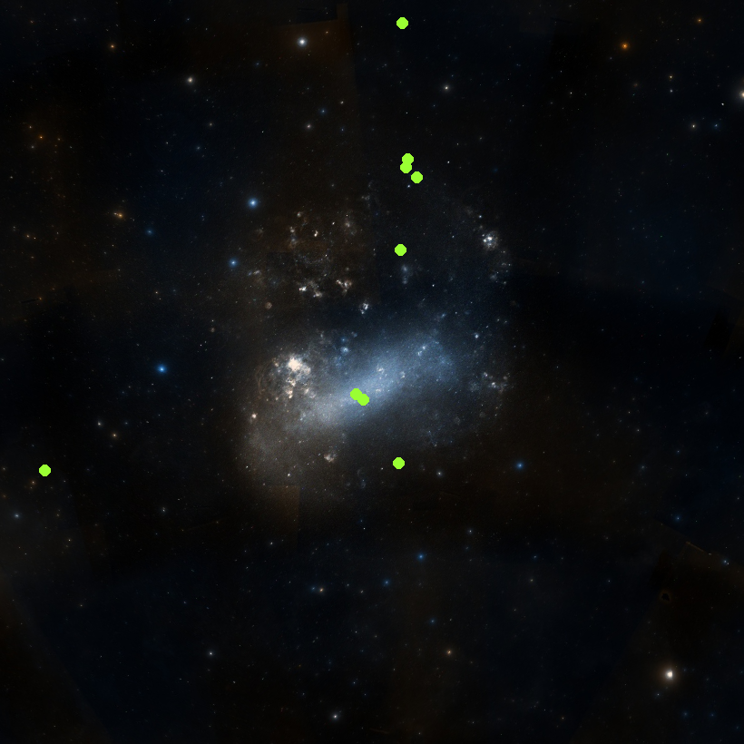
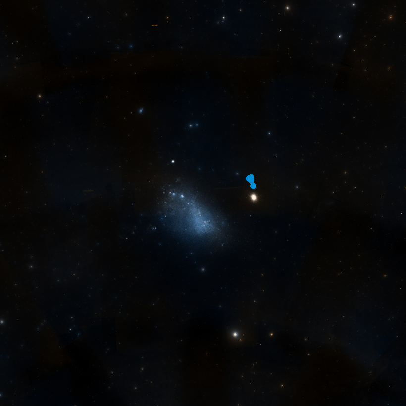
Figure 1: Digitized Sky Survey images of the Magellanic Clouds. Each image is approximately 15^∘ on a side with north at the top and east to the left. Left: Large Magellanic Cloud with the locations of the nine metal-poor giants we followed-up with high-resolution Magellan/MIKE spectroscopy superimposed as green points. Right: Small Magellanic Cloud with the locations of the four metal-poor giants we followed-up with high-resolution Magellan/MIKE spectroscopy superimposed as blue points.

We followed up these 13 stars with the Magellan Inamori Kyocera Echelle (MIKE) spectrograph on the Magellan Clay Telescope at Las Campanas Observatory (Bernstein et al., 2003; Shectman & Johns, 2003). We used either the 0$\farcs$7 or 1$\farcs$0 slits and the standard blue and red grating azimuths, yielding spectra between 335 nm and 950 nm with resolution $R\approx 40,\!000/28,\!000$ in the blue and $R\approx 31,\!000/22,\!000$ in the red for the 0$\farcs$7/1$\farcs$0 slits. We collected all calibration data (e.g., bias, quartz & “milky” flat field, and ThAr lamp frames) in the afternoon before each night of observations. We present a log of these observations in Table 1. We reduced the raw spectra and calibration frames using the CarPy software package (Kelson et al., 2000; Kelson, 2003; Kelson et al., 2014). We used iSpec (Blanco-Cuaresma et al., 2014; Blanco-Cuaresma, 2019) to calculate radial velocities and barycentric corrections and normalized individual orders using IRAF (Tody, 1986, 1993).

Table 1: Log of Magellan/MIKE Observations

2MASS	Galaxy	R.A.	Decl.	UT Date	Start	Slit	Exposure	$v_{r}$	S/N	S/N
Designation		(h:m:s)	(d:m:s)			Width	Time (s)	(km s-1)	$4500\ \rm{\AA}$	$6500\ \rm{\AA}$
J00251849-7140074	SMC	00:25:18.47	-71:40:07.50	2017 Jul 03	07:29:38	1$\farcs$0	03600	$100.5\pm 1.1$	$22$	$45$
J00262394-7128549	SMC	00:26:23.95	-71:28:54.94	2017 Jul 02	08:05:08	1$\farcs$0	14400	$133.7\pm 0.9$	$25$	$60$
J00263959-7122102	SMC	00:26:39.60	-71:22:10.26	2017 Jun 29	07:59:59	1$\farcs$0	03600	$151.3\pm 1.0$	$15$	$31$
J00273753-7125114	SMC	00:27:37.55	-71:25:11.56	2017 Jun 28	09:06:17	1$\farcs$0	03600	$149.4\pm 2.1$	$15$	$47$
J05121686-6517147	LMC	05:12:16.85	-65:17:14.76	2018 Jan 07	05:37:02	1$\farcs$0	03584	$336.2\pm 1.1$	$14$	$50$
J05133509-7109322	LMC	05:13:35.10	-71:09:32.18	2018 Jan 08	04:44:02	1$\farcs$0	05400	$186.9\pm 1.0$	$18$	$45$
J05141665-6454310	LMC	05:14:16.65	-64:54:31.30	2018 Jan 07	00:56:51	1$\farcs$0	19800	$298.9\pm 1.4$	$30$	$65$
J05143154-6505189	LMC	05:14:31.55	-65:05:19.02	2018 Jan 08	03:41:25	1$\farcs$0	03600	$304.3\pm 1.3$	$15$	$35$
J05150380-6647003	LMC	05:15:03.79	-66:47:00.28	2018 Jan 07	04:03:27	1$\farcs$0	05400	$356.8\pm 1.5$	$20$	$60$
J05160009-6207287	LMC	05:16:00.09	-62:07:28.70	2020 Oct 21	07:24:32	1$\farcs$0	06235	$266.0\pm 1.1$	$25$	$60$
J05224088-6951471	LMC	05:22:40.89	-69:51:47.08	2016 Jan 20	01:23:29	0$\farcs$7	17410	$265.3\pm 3.5$	$30$	$75$
J05242202-6945073	LMC	05:24:22.03	-69:45:07.22	2016 Jan 18	01:16:45	0$\farcs$7	25200	$309.0\pm 1.3$	$15$	$50$
J06411906-7016314	LMC	06:41:19.05	-70:16:31.42	2020 Oct 21	04:59:20	1$\farcs$0	07200	$320.3\pm 1.1$	$25$	$76$

3 Stellar Properties

We use both the classical excitation/ionization balance approach and isochrones to infer photospheric stellar parameters for the 13 stars listed in Table 1. Isochrones are especially useful for effective temperature $T_{\text{eff}}$ inferences in this case, as high-quality multiwavelength photometry from the ultraviolet to the mid infrared is available for both the LMC and SMC. Similarly, the known distances of the Magellanic Clouds make the calculation of surface gravity $\log{g}$ via isochrones straightforward. With both $T_{\text{eff}}$ and $\log{g}$ available via isochrones, the equivalent widths of iron lines can be used to self-consistently determine metallicity $[\text{Fe/H}]$ and microturbulence $\xi$.

We follow the algorithm outlined in Reggiani et al. (2020). Using atomic absorption line data from Ji et al. (2020) based on the linemake code (Sneden et al., 2009, 2016) maintained by Vinicius Placco and Ian Roederer, we first measure the equivalent widths of Fe II atomic absorption lines by fitting Gaussian profiles with the splot task in IRAF to our continuum-normalized spectra. We use only Fe II lines with equivalent widths smaller than 150 mÅ in our photospheric stellar parameter inferences to avoid the possibly important effects of departures from local thermodynamic equilibrium (LTE) on Fe I-based inferences. Whenever necessary, we use the deblend task to disentangle absorption lines from adjacent spectral features. We report our input atomic data, measured equivalent widths, and inferred abundances in Table 2.

To evaluate the relative importance of departures from LTE on Fe I- and Fe II-based metallicity inferences, we used the grid of corrections to abundances derived under the assumptions of LTE for departures from LTE (i.e., non-LTE corrections) from Amarsi et al. (2016) for stars with $\log{g}=1.5$. For all of our stars, the non-LTE corrections to our inferred Fe II-based metallicities were less than 0.1 dex and therefore smaller than the overall metallicity uncertainties we adopted. On the other hand, corrections for individual Fe I lines can be as large as 0.3 dex. We therefore argue that the metallicity inference approach we followed based on Fe II lines is likely to be more accurate and precise than one based on Fe I lines.

Table 2: Atomic Data, Equivalent-width Measurements, and Individual-line Abundance Inferences

2MASS	Wavelength	Species	Excitation Potential	log($gf$)	EW	$\log_{\epsilon}(\rm{X})$
Designation	(Å)		(eV)		(mÅ)
J05121686-6517147	$5682.633$	Na I	$2.102$	$-0.706$	$15.50$	$4.166$
J05133509-7109322	$5682.633$	Na I	$2.102$	$-0.706$	$10.00$	$4.090$
J05133509-7109322	$5688.203$	Na I	$2.104$	$-0.406$	$25.20$	$4.250$
J05133509-7109322	$5895.924$	Na I	$0.000$	$-0.194$	$247.30$	$4.287$
J05141665-6454310	$5682.633$	Na I	$2.102$	$-0.706$	$10.10$	$4.240$
J05141665-6454310	$5688.203$	Na I	$2.104$	$-0.406$	$11.00$	$3.982$
J05143154-6505189	$5682.633$	Na I	$2.102$	$-0.706$	$114.60$	$5.534$
J05143154-6505189	$5688.203$	Na I	$2.104$	$-0.406$	$101.80$	$5.081$
J05150380-6647003	$5682.633$	Na I	$2.102$	$-0.706$	$143.40$	$5.597$

Note. — This table is published in its entirety in the machine-readable format. A portion is shown here for guidance regarding its form and content.

We use 1D plane-parallel $\alpha$-enhanced ATLAS9 model atmospheres (Castelli & Kurucz, 2004), the 2019 version of the MOOG radiative transfer code (Sneden, 1973), and the q² MOOG wrapper (Ramírez et al., 2014) to derive with the classical excitation/ionization balance approach an initial set of photospheric stellar parameters $T_{\text{eff}}$, $\log{g}$, $[\text{Fe/H}]$, and $\xi$. Since photospheric stellar parameters inferred via the classical excitation/ionization balance approach differ from those derived using photometry and distance information (e.g., Korn et al., 2003; Mucciarelli & Bonifacio, 2020), we then use the isochrones package (Morton, 2015) in an iterative process to self-consistently infer photospheric and fundamental stellar parameters for each star using as input:

1. photospheric stellar parameters from the classical excitation/ionization balance approach (on the first iteration) or the reduced equivalent width balance approach (on all subsequent iterations);

2. $g$, $r$, $i$, and $z$ magnitudes and associated uncertainties from Data Release (DR) 2 of the SkyMapper Southern Sky Survey (Onken et al., 2019);

3. $J$, $H$, and $K_{\text{s}}$ magnitudes and associated uncertainties from the 2MASS Point Source Catalog (Skrutskie et al., 2006);

4. $W1$ and $W2$ magnitudes and associated uncertainties from the Wide-field Infrared Survey Explorer (WISE) AllWISE Source Catalog (Wright et al., 2010; Mainzer et al., 2011);

5. reddening inferences from Skowron et al. (2021);

6. distances inferred via the surface brightness–color relation for eclipsing binaries in the LMC (Pietrzyński et al., 2019) and SMC (Graczyk et al., 2014). For the SMC, we account for a possibly significant line-of-sight depth inferred by Scowcroft et al. (2016) using the mid-infrared period–absolute magnitude relation for Cepheids (i.e., the Leavitt Law).

We use isochrones to fit the MESA Isochrones and Stellar Tracks (MIST; Dotter, 2016; Choi et al., 2016; Paxton et al., 2011, 2013, 2015, 2018, 2019) library to these data using MultiNest (Feroz & Hobson, 2008; Feroz et al., 2009, 2019). We restrict the MIST library to stellar ages $\tau$ in the range 8.0 Gyr $\leq\tau\leq$ 13.721 Gyr and distances $d$ to the 3-$\sigma$ ranges including both statistical and systematic uncertainties for the LMC and SMC from Pietrzyński et al. (2019) and Graczyk et al. (2014) respectively accounting for the possibly significant line-of-sight depth for the SMC advocated by Scowcroft et al. (2016). We also restrict our analysis to extinctions $A_{V}$ in the ranges proposed by Skowron et al. (2021) at the location of each candidate. While the metal-poor stars in our sample generally have supersolar $\alpha$-element abundances, the current version of the MIST isochrones were calculated using solar-scaled abundances. While this potential inconsistency can affect fundamental stellar parameter inferences like mass and age, the uncertainties due to this effect are usually smaller than the uncertainties resulting from other sources (e.g., Grunblatt et al., 2021).

For the first isochrones calculation, we use in the likelihood the initial set of photospheric stellar parameters inferred from the classical excitation/ionization balance analysis of each spectrum along with the photometric, extinction, and distance information described above. We then use isochrones to calculate a new set of photospheric and fundamental stellar parameters that is both self-consistent and physically consistent with stellar evolution. We next impose the $T_{\text{eff}}$ and $\log{g}$ inferred in this way on an iteration of the reduced equivalent width balance approach to derive $[\text{Fe/H}]$ and $\xi$ values consistent with our measured Fe II equivalent widths and our isochrones inferred $T_{\text{eff}}$ & $\log{g}$. We then execute another isochrones calculation, this time using this updated set of photospheric stellar parameters in the likelihood. We iterate this process until the metallicities inferred from both the isochrones analysis and the reduced equivalent width balance approach are consistent within their uncertainties (typically a few iterations). For our final photospheric stellar parameters, we adopt $T_{\text{eff}}$ and $\log{g}$ from the final isochrones iteration. We infer $A_{V}\approx 1.6$ mag for the two stars coincident with the bar of the LMC 2MASS J05224088-6951471 and 2MASS J05242202-6945073, possibly suggesting that they are on the far side of the LMC.

We prefer stellar parameters inferred using both isochrones and spectroscopy to stellar parameters derived from spectroscopy alone. Isochrone analyses can make use of constraints from multiwavelength photometry as well as distance and extinction information impossible to leverage with the classic spectroscopic method. All of these data are available for the stars in our sample. Unlike $T_{\text{eff}}$ and $\log{g}$ values derived from spectroscopy alone, $T_{\text{eff}}$ and $\log{g}$ values deduced from isochrone analyses are guaranteed to be self-consistent and in principle realizable during stellar evolution (to the degree of accuracy achievable in by the stellar models). It has long been known that photospheric stellar parameters inferred for metal-poor giants using the classical approach differ from those derived using photometry and parallax information (e.g., Korn et al., 2003; Frebel et al., 2013; Mucciarelli & Bonifacio, 2020). Since LTE is almost always assumed in the calculation of the model atmospheres used to interpret equivalent width measurements, these differences are often attributed to the violation of the assumptions of LTE in the photospheres of metal-poor giants.

We derive the uncertainties in our adopted $[\text{Fe/H}]$ and $\xi$ values due to the uncertainties in our adopted $T_{\text{eff}}$ and $\log{g}$ values using a Monte Carlo simulation. We randomly sample self-consistent pairs of $T_{\text{eff}}$ and $\log{g}$ from our isochrones posteriors and calculate the values of $[\text{Fe/H}]$ and $\xi$ that produce the best reduced equivalent width balance given our Fe II equivalent width measurements. We save the result of each iteration and find that the contributions of $T_{\text{eff}}$ and $\log{g}$ uncertainties to our final $[\text{Fe/H}]$ and $\xi$ uncertainties are small: about 0.01 dex for both the LMC and SMC. We derive our adopted metallicities and uncertainties using a final reduced equivalent width balance calculation imposing the adopted $T_{\text{eff}}$ and $\log{g}$ values described above. The result of this calculation agrees well with the result of the Monte Carlo simulation. We report our adopted photospheric stellar parameters both by themselves in Table 3 and together with all of our derived stellar parameters in the comprehensive Table 4.

We define the line-by-line dispersion of our inferred iron abundances as the standard deviation of the Fe II abundances inferred from individual Fe II lines. The uncertainties in our metallicity inferences are dominated by this line-by-line dispersion. We provide in Tables 3 and 4 our adopted Fe II-based metallicities with uncertainties derived by adding in quadrature the relatively large uncertainties from our line-by-line abundance dispersions and the relatively small uncertainties that can be attributed to $T_{\text{eff}}$ and $\log{g}$ uncertainties. We also present in Table 4 a detailed view of our adopted photospheric and fundamental stellar parameters for all 13 stars in our LMC and SMC samples. All of the uncertainties quoted in Table 4 include random uncertainties only. That this, they are uncertainties derived under the unlikely assumption that the MIST isochrone grid we use in our analyses perfectly reproduces all stellar properties.

Table 3: Adopted Photospheric Stellar Parameters

2MASS	$T_{\text{eff}}$	$\log{g}$	$[\text{Fe/H}]$	$\xi$
Designation	(K)			(km s-1)
J00251849-7140074	$4372^{+5}_{-3}$	$0.65\pm 0.01$	$-2.33\pm 0.30$	$2.71\pm 0.50$
J00262394-7128549	$4388^{+8}_{-6}$	$0.87\pm 0.01$	$-2.02\pm 0.32$	$2.51\pm 0.80$
J00263959-7122102	$4481^{+2}_{-1}$	$0.73\pm 0.01$	$-2.60\pm 0.39$	$3.01\pm 0.45$
J00273753-7125114	$4326\pm 10$	$0.61\pm 0.01$	$-2.27\pm 0.26$	$3.83\pm 0.95$
J05121686-6517147	$4247\pm 1$	$0.55\pm 0.01$	$-2.32\pm 0.36$	$2.91\pm 0.50$
J05133509-7109322	$4520^{+26}_{-18}$	$1.06\pm 0.02$	$-2.15\pm 0.38$	$2.55\pm 0.75$
J05141665-6454310	$4761^{+18}_{-15}$	$1.43\pm 0.02$	$-2.42\pm 0.23$	$2.45\pm 0.62$
J05143154-6505189	$4361^{+2}_{-1}$	$1.06\pm 0.01$	$-1.65\pm 0.35$	$2.74\pm 0.83$
J05150380-6647003	$4139^{+14}_{-13}$	$0.64\pm 0.02$	$-1.83\pm 0.46$	$3.31\pm 0.91$
J05160009-6207287	$4151\pm 17$	$0.60\pm 0.02$	$-1.62\pm 0.24$	$3.25\pm 0.54$
J05224088-6951471	$4619^{+45}_{-23}$	$1.24\pm 0.03$	$-2.14\pm 0.32$	$3.16\pm 0.45$
J05242202-6945073	$4903^{+31}_{-49}$	$1.61\pm 0.03$	$-1.99\pm 0.47$	$2.38\pm 0.78$
J06411906-7016314	$4093^{+8}_{-7}$	$0.53\pm 0.01$	$-1.54\pm 0.14$	$3.28\pm 0.47$

Note. — We give our adopted photospheric stellar parameters both by themselves here and in our comprehensive table of stellar parameters in Table 4.

To roughly quantify the magnitude of the possible photospheric stellar parameter systematic uncertainties resulting from our analysis, we compared our photospheric stellar parameters with those inferred by APOGEE’s ASPCAP for the two stars 2MASS J05160009-6207287 and 2MASS J06411906-7016314 in our sample selected from SDSS DR16 (Ahumada et al., 2020). Our photospheric stellar parameters are consistent with those produced by ASPCAP, as the differences in $T_{\text{eff}}$, $\log{g}$, and $[\text{Fe/H}]$ are 15 K, 0.1 dex, and 0.01 dex, fully consistent within the ASPCAP reported uncertainties ($\pm 100$ K, $\pm 0.1$ dex, and $\pm 0.03$ dex). The excellent agreement between these two analyses suggests that any systematic uncertainties in our photospheric stellar parameters resulting from our analysis procedure are small.

4 Elemental Abundances

To infer the elemental abundances of several $\alpha$, light odd-$Z$, iron-peak, and neutron-capture elements, we first measure the equivalent widths of atomic absorption lines of Na I, Mg I, Si I, Ca I, Sc II, Ti I, Ti II, Cr I, Mn I, Co I, Ni I, Y II, Ba II, La II, Ce II, Nd II, Sm II, and Gd II in our continuum-normalized spectra by fitting Gaussian profiles with the splot task in IRAF. We use the deblend task to disentangle absorption lines from adjacent spectral features whenever necessary. We measure an equivalent width for every absorption line in our line list that could be recognized, taking into consideration the quality of a spectrum in the vicinity of a line and the availability of alternative transitions of the same species. If possible we avoid lines bluer than 4500 Å, as the signal-to-noise ratios (S/N) in our spectra blueward of 4500 Å are poor. Blueward of 5000 Å in MIKE’s blue arm we were able to measure equivalent widths of lines with equivalent widths greater than 10 mÅ. Redward of 5000 Å in MIKE’s red arm, we were able to measure equivalent widths of lines with equivalent widths greater than 5 mÅ. These limiting S/N ratios applied even to our lower S/N stars. In a few cases we measured lines with smaller EWs for species without other available lines. Whenever possible, we avoid saturated lines like Mg I $b$ as well. We consider hyperfine splitting in our abundance inferences for Mn I, Co I, and Y II. We account for isotopic splitting in barium using data from McWilliam (1998) for the three Ba II lines at $5853$, $6141$, and $6496$ Å that we use for our barium abundance inferences. We use the 1D plane-parallel $\alpha$-enhanced ATLAS9 model atmospheres and the 2019 version of MOOG to infer elemental abundances based on each equivalent width measurement. We use spectral synthesis to infer the abundance of Eu II, mostly from its 6645 Å line. Although this line is not usually strong, it is clearly measurable in 10 of the 13 giants in our sample. For the most europium-poor star in our sample 2MASS J05141665-6454310, we used the Eu II line at 4129 Å for our abundance inference.

We report our input atomic data, measured equivalent widths, and the abundances and associated uncertainties we derive in Table 2. We present in Table 5 our adopted mean elemental abundances and associated uncertainties defined as the quadrature sum of the line-by-line abundance dispersions and the uncertainties that result from our photospheric stellar parameter uncertainties. We indicate typical uncertainties in each panel of Figures 2 to 4. Our iterative use of both isochrones and the classical excitation/ionization balance approach to stellar parameter inference produced very precise stellar parameters, and that precision is reflected in the abundance uncertainties we report in Table 5.

As we described in Section 3, we have not accounted for the possibility of systematic uncertainties in our stellar parameter inferences. To quantify the effect of possible systematic uncertainties in our stellar parameter inferences on our abundance inferences, we recalculated our abundances assuming $T_{\text{eff}}$ and $\log{g}$ uncertainties $\Delta T_{\text{eff}}=100$ K and $\Delta\log{g}=0.1$ dex. However, the effect of these inflated stellar parameter uncertainties is small because our abundance uncertainties are dominated by our metallicity uncertainties.

To present a more complete view of the Magellanic Clouds’ metal-poor stellar populations, we also plot in Figures 2 to 4 the abundances of stars in LMC inner disk/bar fields (Pompéia et al., 2008; Van der Swaelmen et al., 2013) as well as the abundances of stars in both the LMC and SMC observed by SDSS-IV/APOGEE-2 made available as part of SDSS DR 16 (e.g., Nidever et al., 2020). For the latter sample, to focus on LMC and SMC members we use the heliocentric radial velocity and proper motion cuts proposed by Nidever et al. (2020) using the APOGEE spectra themselves and Gaia DR2 astrometry (Gaia Collaboration et al., 2016, 2018; Salgado et al., 2017; Arenou et al., 2018; Lindegren et al., 2018; Luri et al., 2018). We do not segregate the SDSS DR16 Magellanic Clouds sample into individual LMC/SMC samples, as Nidever et al. (2020) suggested that both galaxies have similarly delayed chemical evolution histories (especially at metallicities below $[\text{Fe/H}]\sim-2$).

4.1 $\alpha$ Elements

Magnesium, silicon, calcium, and titanium are often referred to as $\alpha$ elements. While magnesium and calcium are indeed synthesized by the fusion of existing nuclei and $\alpha$ particles, silicon is formed during both hydrostatic and explosive oxygen burning. Likewise, titanium is a product of both explosive oxygen and silicon burning. Silicon and titanium are still usually included as $\alpha$ elements though, because the chemical evolution of $[\text{Si/Fe}]$ and $[\text{Ti/Fe}]$ as functions of $[\text{Fe/H}]$ are similar to that of magnesium and calcium (e.g., Nomoto et al., 2006; Clayton, 2007; Wongwathanarat et al., 2017).

We plot in Figure 2 our inferred LTE $[\alpha/\text{Fe}]$ abundances as a function of $[\text{Fe/H}]$. We find that our inferred magnesium, calcium, and titanium abundances are consistent with the $\alpha$-enhanced abundances observed in metal-poor Milky Way stars. This is true both for our LMC and SMC samples. As we argue below, among the $\alpha$ elements we studied our magnesium abundance inferences are likely to be least effected by departures from the assumptions of LTE. In the Fe II-based metallicity range spanned by our Magellanic Clouds sample $-2.6\lesssim[\text{Fe/H}]\lesssim-1.5$, the 16th, 50th, and 84th percentiles of our $[\text{Mg/Fe}]$ distribution are $[\text{Mg/Fe}]$ = 0.10, 0.37, and 0.53. For the 113 Milky Way halo stars from Roederer et al. (2014) in the same Fe II-based metallicity range, the 16th, 50th, and 84th percentiles of the $[\text{Mg/Fe}]$ distribution are $[\text{Mg/Fe}]$ = 0.10, 0.26, and 0.41. In other words, the 1-$\sigma$ ranges of the two distributions are consistent. While our sample size is too small to apply the two-sided Kolmogorov-Smirnov test often used to assess whether or not there is reason to believe that two samples were produced by the same parent distribution, we nevertheless performed the calculation and found a $p$-value = 0.895. This result gives us no reason to believe that the Magellanic Clouds $[\text{Mg/Fe}]$ distribution is distinct from that of the Milky Way in the same metallicity range. Applying these same steps to calcium and titanium produce the same result and give us no reason to believe that their distributions are distinct from that of the Milky Way in the same metallicity range. The high abundances of magnesium and calcium we infer are also in agreement with the increase in $[\alpha/\text{Fe}]$ with decreasing $[\text{Fe/H}]$ observed in the Magellanic Clouds comparison sample at higher metallicities.

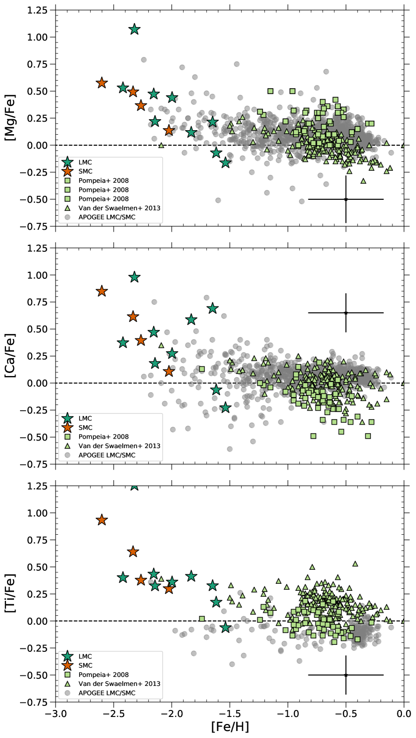
Figure 2: Abundances of titanium and the $\alpha$ elements magnesium and calcium relative to iron. We plot as dark green stars our nine LMC giants and as orange stars our four SMC giants. We plot as light green squares LMC inner disk giants from Pompéia et al. (2008) and as light green triangles LMC bar giants from Van der Swaelmen et al. (2013). We plot as gray circles LMC and SMC giants observed by SDSS-IV/APOGEE-2 that are part of SDSS DR16 (e.g., Nidever et al., 2020). In the bottom-left titanium panel, for the SDSS DR16 comparison sample we plot as points average Ti I and Ti II values only for stars with both Ti I and Ti II inferences. The point with error bars in a corner of each panel corresponds to the averaged uncertainty of our complete 13 star sample. Like stars in the Milky Way and M31, we find that in the range $-2.6\lesssim[\text{Fe/H}]\lesssim-2.0$ LMC and SMC giants both have supersolar $[\alpha/\text{Fe}]$ abundance ratios indicative of formation in an environment in which thermonuclear supernovae had not yet contributed significantly to chemical evolution.

For the two stars in common between our sample and SDSS2 DR16, we compared our $\alpha$-element abundances with those produced by ASPCAP with no bad data or warning flags. For $[\text{Mg/Fe}]$ and $[\text{Ca/Fe}]$, both sets of abundances are consistent within the uncertainties. For $[\text{Si/Fe}]$, our abundances are higher than the ASPCAP abundances.

Our inferred magnesium and calcium abundances are unlikely to be significantly affected by departures from the assumptions of LTE. Non-LTE corrections for LTE magnesium abundances from the INSPECT project based on the results of Osorio & Barklem (2016) are about $-0.03$ dex for the magnesium lines we used and the photospheric stellar parameters of the stars in our sample These corrections are too small to affect any of our conclusions based on magnesium abundances. Non-LTE corrections for LTE silicon abundances $[\text{Si/Fe}]\lesssim 0.8$ based on the Amarsi & Asplund (2017) correction grid are about $-0.02$ dex. For stars with abundances $[\text{Si/Fe}]\gtrsim 0.8$ dex, non-LTE corrections can be as large as $-0.2$ dex. Correcting for departures from LTE would therefore decrease the dispersion in $[\text{Si/Fe}]$ for our sample. Non-LTE corrections for LTE calcium abundances based on the Amarsi et al. (2020) correction grid are about $-0.1$ for metal-poor giants. Non-LTE corrections for titanium can be as large as $+0.2$ dex (e.g., Bergemann, 2011), but grids of corrections for titanium are not currently available. Overall, we argue that magnesium is the $\alpha$ element in our sample least effected by possible departures the assumptions of LTE.

4.2 Light Odd-$Z$ and Iron-peak Elements

While sodium is mostly produced in core-collapse supernovae, sodium yields are dependent on metallicity and consequently its chemical evolution is not as easily interpreted as the chemical evolution of the $\alpha$ elements. Both the exact nucleosynthetic origin and chemical evolution of scandium and potassium are likewise hard to identify and interpret (e.g., Clayton, 2007). We plot in the top panels of Figure 3 our measured $[\text{Na/Fe}]$ and $[\text{Sc/Fe}]$ abundances as a function of $[\text{Fe/H}]$. The dispersions in our inferred $[\text{Na/Fe}]$ abundances are considerably higher than the $\alpha$ element dispersion depicted in Figure 2. This is a common occurrence in studies of metal-poor stars and is also observed at higher metallicities in the Pompéia et al. (2008), Van der Swaelmen et al. (2013), and SDSS DR16 comparison samples. Our scandium abundance inferences have a dispersion comparable to the $\alpha$ element dispersion depicted in Figure 2. For the two stars in common between our sample and SDSS DR16, we compared our light odd-$Z$ abundances with those produced by ASPCAP with no bad data or warning flags. Both sets of abundances are consistent within the uncertainties for $[\text{K/Fe}]$, while for $[\text{Na/Fe}]$ the ASPCAP abundances are slightly larger than our abundances.

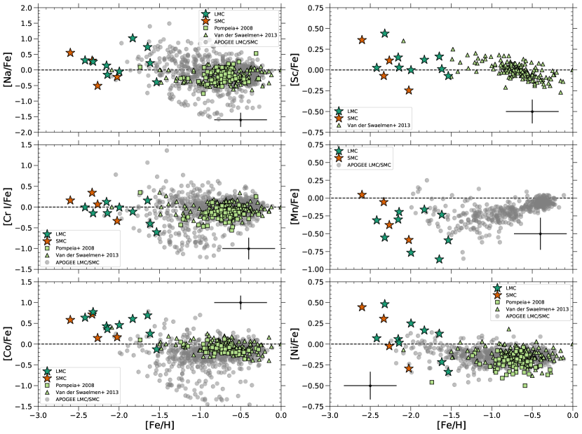
Figure 3: Abundances of light odd-$Z$ elements sodium and scandium plus iron-peak elements chromium, manganese, cobalt, and nickel. We plot as dark green stars our nine LMC giants and as orange stars our four SMC giants. We plot as light green squares LMC inner disk giants from Pompéia et al. (2008) and as light green triangles LMC bar giants from Van der Swaelmen et al. (2013). We plot as gray circles LMC and SMC giants observed by SDSS-IV/APOGEE-2 that are part of SDSS DR16 (e.g., Nidever et al., 2020). The point with error bars in a corner of each panel corresponds to the mean uncertainty of our complete 13 star sample. Aside from elevated cobalt abundances that can be attributed to enrichment from hypernovae, the light odd-$Z$ and iron-peak abundances we infer are as expected for metal-poor giants in the Milky Way and its dSph galaxies.

While sodium and potassium abundance inferences can be strongly affected by departures from LTE, scandium abundances from Sc II lines are not strongly affected by departures from LTE (e.g., Zhao et al., 2016). Because our comparison samples did not correct for departures from LTE or derive potassium abundances, we plot in Figure 3 LTE sodium abundances and do not plot our potassium abundances. In Table 5 we report our sodium and potassium abundances inferred both under the assumptions of LTE and corrected for the departures from LTE. We sourced sodium abundance corrections based on Lind et al. (2011) through the INSPECT project. We obtained potassium abundance corrections via a linear interpolation of the Reggiani et al. (2019) grid of corrections for abundances inferred from the equivalent width of the K I line at 7698 Å.

Iron-peak elements are primarily synthesized in thermonuclear supernovae. The chemical evolution of chromium and nickel trace the evolution of iron, so the nucleosynthetic origins of these elements are thought to be similar. We plot in the bottom panels of Figure 3 our inferred $[\text{Cr/Fe}]$, $[\text{Mn/Fe}]$, $[\text{Co/Fe}]$, and $[\text{Ni/Fe}]$ abundances as a function of $[\text{Fe/H}]$. In metal-poor Milky Way stars, both $[\text{Cr/Fe}]$ and $[\text{Ni/Fe}]$ are often observed in solar abundance ratios. In dSph galaxies though, significantly non-solar $[\text{Cr/Fe}]$ and $[\text{Ni/Fe}]$ are sometimes found (e.g., Ji et al., 2016b). While there is some evidence for supersolar $[\text{Ni/Fe}]$ abundances and significant $[\text{Mn/Fe}]$ scatter in our metal-poor Magellanic Cloud giants, the possible offsets are small relative to our abundance uncertainties. The cobalt abundances of the metal-poor giants in our Magellanic Clouds sample are considerably higher than those of the comparison samples. This is not surprising, as it is known that there is a sharp increase in cobalt abundances with decreasing metallicity (e.g., Cayrel et al., 2004; Reggiani et al., 2017, 2020). Because cobalt nucleosynthesis is dependent on core-collapse supernovae explosion energy, the abundance increase with decreasing metallicity could be due to enrichment by hypernovae (e.g. Clayton, 2007; Kobayashi et al., 2006, 2020). However, this commonly observed feature is still not reproduced by many recent chemical evolution models (e.g., Prantzos et al., 2018; Kobayashi et al., 2020). Zinc abundance inferences for these stars might help isolate the origin of this enhancement. For the two stars in common between our sample and SDSS DR16, we compared our iron-peak abundances with those produced by ASPCAP with no bad data or warning flags. For $[\text{Cr/Fe}]$ and $[\text{Ni/Fe}]$, both sets of abundances are consistent within the uncertainties.

Our inferred iron-peak abundances are unlikely to be significantly affected by departures from the assumptions of LTE. While chromium abundances can be strongly affected by departures from the assumptions of LTE with non-LTE corrections as large as +0.5 dex for metal-poor giants (e.g., Bergemann & Cescutti, 2010), our chromium abundances are consistent with our comparison samples. Non-LTE manganese corrections for metal-poor giants are about +0.2 dex (e.g., Amarsi et al., 2020), comparable to our inferred manganese uncertainties.

4.3 Neutron-capture Elements

Elements with atomic numbers beyond zinc are mostly produced by neutron-capture processes either “slow” or “rapid” relative to $\beta$ decay timescales. The relative contributions of these $s$- and $r$-processes to the nucleosynthesis of each neutron-capture element are functions of metallicity. Some elements like yttrium and barium are commonly used as tracers of the $s$-process, while europium is the most easily observed element thought to be produced exclusively in the $r$-process (e.g., Cescutti et al., 2006; Jacobson & Friel, 2013; Ji et al., 2016a).

We plot in Figure 4 our inferred neutron-capture element abundances as a function of $[\text{Fe/H}]$. The abundances of the $s$-process elements yttrium and barium inferred from Y II and Ba II lines are normal. $[\text{Y/Fe}]$ abundances clustered near the solar value are commonly observed in metal-poor Milky Way giants. Likewise, subsolar $[\text{Ba/Fe}]$ abundances are not uncommon and are frequently observed in metal-poor Milky Way stars in both the halo and bulge (e.g., Reggiani et al., 2017, 2020; Prantzos et al., 2018; Kobayashi et al., 2020).

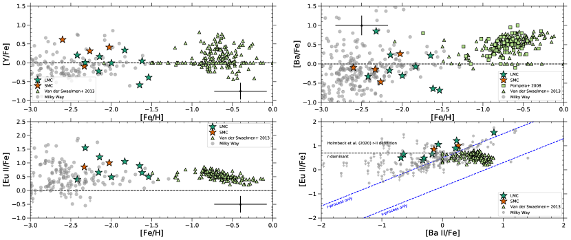
Figure 4: Abundances of neutron-capture elements yttrium, barium, and europium. We plot as dark green stars our nine LMC giants and as blue stars our four SMC giants. We plot as light green squares LMC inner disk giants from Pompéia et al. (2008) and as light green triangles LMC bar giants from Van der Swaelmen et al. (2013). We plot as gray circles metal-poor Milky Way giants from Barklem et al. (2005) and Jacobson et al. (2015) selected for high-resolution follow-up observations without regard to their $r$-process abundances. The point with error bars in a corner of each panel corresponds to the mean uncertainty of our complete 13 star sample. In the metallicity range $-2.6\lesssim[\text{Fe/H}]\lesssim-1.5$, relative to the Milky Way the $[\text{Eu/Fe}]$ abundances of the giants stars in our Magellanic Clouds sample are uniformly high with an increased occurrence of r-II stars with $[\text{Eu/Fe}]\geq 1.0$ and $[\text{Eu/Ba}]\geq 0$. The stars consistently have $[\text{Eu/Ba}]$ abundances indicative of $r$-process nucleosynthesis.

Our inferred abundances of the $r$-process element europium in metal-poor Magellanic Cloud giants are remarkable. Most extraordinary are the $[\text{Eu/Fe}]\approx 1.5$ abundances observed in the stars 2MASS J05121686-6517147 and 2MASS J05224088-6951471. In Figure 5 we show europium lines at 6645 Å to illustrate their large equivalent widths and therefore the large abundances of europium in our sample. The occurrence of so-called r-II stars is very high in our sample of metal-poor Magellanic Cloud giants. Indeed, three of our nine metal-poor LMC giants are significantly enhanced in europium according to the classical definition of r-II stars (i.e., $[\text{Eu/Fe}]\geq 1.0$ and $[\text{Eu/Ba}]\geq 0$) from Beers & Christlieb (2005). If instead we adopt the new empirical r-II classification (i.e., $[\text{Eu/Fe}]\geq 0.7$) proposed by Holmbeck et al. (2020), then six out of our nine metal-poor LMC giants are r-II stars (with two more at $[\text{Eu/Fe}]=0.65$ and and $[\text{Eu/Fe}]=0.50$ very close to the defined limit). Regardless of which classification we adopt, all nine of our LMC giants are considered r-I stars (i.e., $[\text{Eu/Fe}]\geq 0.3$) and therefore $r$-process enhanced. While we were only able to infer europium abundances for two of our four metal-poor SMC giants, one is an r-II star according to Beers & Christlieb (2005) while both are r-II stars according to Holmbeck et al. (2020). While we see elevated $[\text{Eu/Fe}]$ abundances in the metallicity range $-2.6\lesssim[\text{Fe/H}]\lesssim-1.8$, at higher metallicities $[\text{Eu/Fe}]$ levels off close to the values observed in the Milky Way at similar metallicities (e.g., Van der Swaelmen et al., 2013; Kobayashi et al., 2020).

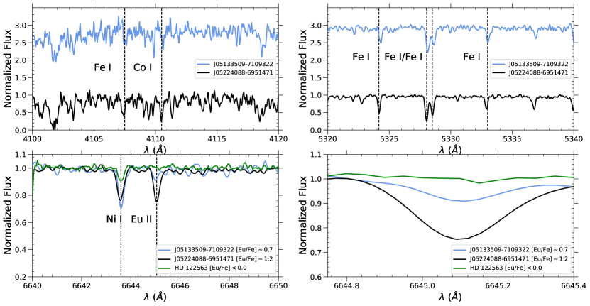
Figure 5: Spectra for two LMC giants in our sample 2MASS J05133509-7109322 ($[\text{Eu/Fe}]\approx 0.6$) and 2MASS J05224088-6951471 ($[\text{Eu/Fe}]\approx 1.5$) plus the well-studied metal-poor giant HD 122563 ($[\text{Eu/Fe}]\lesssim 0$). All three stars have similar similar photospheric stellar parameters, and 2MASS J05133509-7109322 & 2MASS J05224088-6951471 span our S/N range. Top left: spectra in the blue in the wavelength range 4100 Å $\leq\lambda\leq$ 4120 Å. Top right: spectra in the green in the wavelength range 5320 Å $\leq\lambda\leq$ 5340 Å. Bottom left: spectra in the red in the wavelength range 6640 Å $\leq\lambda\leq$ 6650 Å in the vicinity of the Eu II line at 6645 Å. Bottom right: close-up view of the Eu II line at 6645 Å.

Among the neutron-capture abundances we inferred, grids of non-LTE corrections are only readily available for barium. Non-LTE barium corrections for metal-poor giants are about $-0.1$ dex (e.g., Amarsi et al., 2020).

5 Discussion

In both the Large and Small Magellanic Clouds, in the metallicity interval $-2.6\lesssim[\text{Fe/H}]\lesssim-2.0$ we observe high average values of $[\text{Eu/Fe}]$, increased occurrences of $r$-process enhanced stars relative to the Milky Way, and $\alpha$ element enhancements. To quantify the significance of these first two observations, we compare our results with the distribution of Milky Way halo $[\text{Eu/Fe}]$ abundances observed by Barklem et al. (2005) and Jacobson et al. (2015) in the same range of metallicity. Since our sample was selected independently of $[\text{Eu/Fe}]$, it should provide an unbiased view of the Magellanic Clouds’ $[\text{Eu/Fe}]$ distribution in the metallicity range $-2.6\lesssim[\text{Fe/H}]\lesssim-1.5$. Likewise, the stars observed by Barklem et al. (2005) and Jacobson et al. (2015) were selected without regard to their $[\text{Eu/Fe}]$ abundances, so the union of the Barklem et al. (2005) and Jacobson et al. (2015) catalogs provides an unbiased view of the distribution of $[\text{Eu/Fe}]$ in Milky Way halo stars in the metallicity range $-2.6\lesssim[\text{Fe/H}]\lesssim-1.5$. Because all of the stars in our Magellanic Clouds sample have $[\text{Eu/Ba}]\geq 0$ as expected from $r$-process nucleosynthesis, we first remove all stars from the Barklem et al. (2005) and Jacobson et al. (2015) catalogs with $[\text{Eu/Ba}]<0$. From here, we refer to this sample as our control sample.

For each of the nine stars in our LMC sample, we calculate the probability $p_{i}$ that a randomly selected star from the control sample with $|[\text{Fe/H}]_{\text{LMC}}-[\text{Fe/H}]_{\text{control}}|<\sigma_{[\text{Fe/H}]}$ has $[\text{Eu/Fe}]_{\text{control}}\geq[\text{Eu/Fe}]_{\text{LMC}}$. We then use these individual probabilities to calculate the probability $9!\prod_{i=1}^{9}p_{i}$ that a nine-star sample from the control sample has a more extreme $[\text{Eu/Fe}]$ distribution than what we observe in the LMC. We find that random sampling from the control $[\text{Eu/Fe}]$ distribution has only a 1 in 20600 chance of producing the extreme $[\text{Eu/Fe}]$ we observe in the LMC, equivalent to a 3.90-$\sigma$ offset. A similar calculation for the two SMC stars for which were able to infer $[\text{Eu/Fe}]$ indicates that random sampling from the control $[\text{Eu/Fe}]$ distribution has only a 1 in 279 chance of producing the extreme $[\text{Eu/Fe}]$ distribution we observe in the SMC, equivalent to a 2.69-$\sigma$ offset. Overall, we find that random sampling from the control $[\text{Eu/Fe}]$ distribution has only a 1 in $2.88\times 10^{6}$ chance of producing the extreme $[\text{Eu/Fe}]$ distribution we observe in the metal-poor Magellanic Clouds sample, equivalent to a 4.96-$\sigma$ offset.

All 11 metal-poor Magellanic Cloud giants for which we could infer a europium abundance would be classified as r-I or r-II stars according to the criteria proposed by Beers & Christlieb (2005). We find that three of nine metal-poor LMC giants would be classified as r-II stars according to Beers & Christlieb (2005); six would be classified as r-II stars according to Holmbeck et al. (2020). Both metal-poor SMC giants for which we could infer europium abundances would be considered r-II stars according to Holmbeck et al. (2020); only one would be considered an r-II star according to Beers & Christlieb (2005). If we model the occurrence of $r$-process enhanced stars with a binomial distribution and use an uninformative Beta(1,1) prior in a Bayesian analysis, then the posterior on occurrence will have a Beta distribution as well. We thereby find in the metallicity range $-2.6\lesssim[\text{Fe/H}]\lesssim-1.5$ r-I occurrence rates in the LMC, SMC, and complete Magellanic Cloud samples to be $93^{+5}_{-10}$%, $79^{+15}_{-25}$%, and $94^{+4}_{-9}$%. According to the Beers & Christlieb (2005) definition, we find in the same metallicity range r-II occurrence rates in the LMC, SMC, and complete Magellanic Cloud samples to be $36^{+15}_{-14}$%, $50^{+25}_{-25}$%, and $38^{+14}_{-13}$%. According to the Holmbeck et al. (2020) definition, we find in the same metallicity range r-II occurrences in the LMC, SMC, and complete Magellanic Cloud samples to be $64^{+14}_{-15}$%, $79^{+15}_{-25}$%, and $70^{+12}_{-14}$%.

The occurrence rates of $r$-process enhanced stars we observe in the Magellanic Clouds are significantly higher than in the halo of the Milky Way or most ultra-faint dSph galaxies. Barklem et al. (2005) found that 14%/3% of metal-poor Milky Way halo stars are classified as r-I/r-II according to the Beers & Christlieb (2005) definitions. More recent estimates by the $r$-process Alliance have found similar occurrences (e.g., Hansen et al., 2018; Sakari et al., 2018). We note that while Ezzeddine et al. (2020) report somewhat higher rates of $r$-process enhancement, even their possibly biased input sample still produces significantly lower occurrences of both r-I and r-II stars than what we observe in the Magellanic Clouds. The ultra-faint dSph galaxies Reticulum II and Tucana III are the only environments in which similar occurrences of $r$-process enhanced stars have been found (e.g., Ji et al., 2016a, b; Roederer et al., 2016; Hansen et al., 2017; Marshall et al., 2019).

In addition to their enhancements in $[\text{Eu/Fe}]$, in the metallicity range $-2.6\lesssim[\text{Fe/H}]\lesssim-2.0$ all of our metal-poor giants in the LMC and SMC giants are also enhanced in the $\alpha$ elements. These elevated $[\alpha/\text{Fe}]$ abundances are indicative of formation by a time at which thermonuclear supernovae had not yet started contributing significantly to the Magellanic Clouds’ stellar populations’ chemical evolution (e.g., Tinsley, 1979). The implication is that the metal-poor LMC and SMC giants in our sample formed after the Magellanic Clouds’ first core-collapse supernovae but before thermonuclear supernovae could contribute significantly to the Magellanic Clouds’ chemical evolution. The copious iron-peak nucleosynthesis produced in thermonuclear supernovae causes $[\alpha/\text{Fe}]$ to decline, and the metallicity at which $[\alpha/\text{Fe}]$ transitions from a high and constant value to a linearly decreasing function of metallicity is often called the “knee” in the $[\text{Fe/H}]$—$[\alpha/\text{Fe}]$ plane.

While the scenario outlined above is likely too simplistic and the metallicity at which $[\alpha/\text{Fe}]$ declines depends on stellar and supernovae feedback, outflows, and inflows, $[\alpha/\text{Fe}]$ tends to begin its decline at higher metallicities in more massive galaxies (e.g., Suda et al., 2017; Nidever et al., 2020). The Magellanic Clouds appear to be an outlier in this regard, as it has been argued that in the Magellanic Clouds $[\alpha/\text{Fe}]$ begins its decline below $[\text{Fe/H}]\approx-2.2$ (Nidever et al., 2020). These upper limits are below the metallicities at which $[\alpha/\text{Fe}]$ begins to decline in less massive galaxies like Sagittarius, Fornax, and Sculptor, though we acknowledge that the $\alpha$-abundance plateaus in these galaxies are are not as clearly defined as in the Milky Way (e.g. Kirby et al., 2011b). Indeed, if the Magellanic Clouds followed the trends with mass observed in Sagittarius, Fornax, and Sculptor then $[\alpha/\text{Fe}]$ should start to decline in the Magellanic Clouds at $[\text{Fe/H}]\approx-1.2$ (e.g., Nidever et al., 2020).

Our stars extend to lower metallicities than most of the Magellanic Cloud stars studied by Nidever et al. (2020), and we therefore attempted to locate the metallicity at which $[\alpha/\text{Fe}]$ begins to decline in the Magellanic Clouds. To algorithmically search for the knee in the Magellanic Clouds’ $[\text{Fe/H}]$—$[\alpha/\text{Fe}]$ distribution, we use the segmented (Muggeo, 2003) package in R (R Core Team, 2020) to fit a segmented piece-wise linear model to the $[\text{Fe/H}]$ and $[\text{Mg/Fe}]$ values presented in Figure 2. For our point estimates, the best fit piece-wise linear model features a declining $[\text{Mg/Fe}]$ trend in the $[\text{Fe/H}]$—$[\text{Mg/Fe}]$ plane, even at $[\text{Fe/H}]\approx-2.6$. We were unable to identify a plateau at constant $[\text{Mg/Fe}]$ at low metallicity using the combination of our observations and SDSS DR16 data, so it is difficult to interpret this result according to the Tinsley (1979) paradigm. We also used a Monte Carlo simulation to investigate the impact of our $[\text{Fe/H}]$ and $[\text{Mg/Fe}]$ uncertainties on our inferences about the knee. On each iteration of our Monte Carlo simulation, we sampled values of $[\text{Fe/H}]$ and $[\text{Mg/Fe}]$ from normal distributions assuming the uncertainties given in Table 5. We then fit a segmented piece-wise linear model to the $[\text{Fe/H}]$ and $[\text{Mg/Fe}]$ values produced in each iteration and saved the result. While our $[\text{Fe/H}]$ and $[\text{Mg/Fe}]$ uncertainties limit our ability to precisely infer segment slopes and end points, we never observed a plateau at constant $[\text{Mg/Fe}]$ at low metallicity. We plot the results of these calculations in Figure 6.

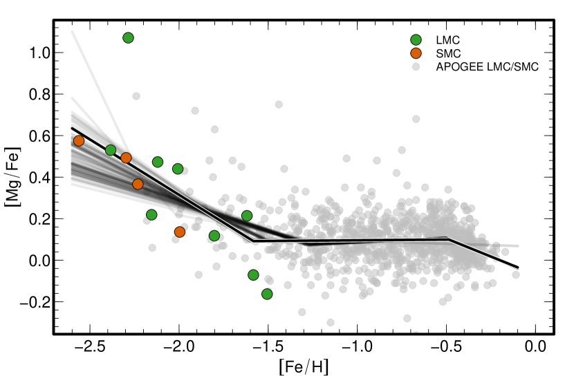
Figure 6: Evolution of $[\text{Mg/Fe}]$ with $[\text{Fe/H}]$ in the Magellanic Clouds. We plot as dark green circles our nine LMC giants and as blue circles our four SMC giants. We plot as gray circles LMC and SMC giants observed by SDSS-IV/APOGEE-2 that are part of SDSS DR16 (e.g., Nidever et al., 2020). The opaque black line is the best-fit three-segment linear model for our point estimates of $[\text{Fe/H}]$ and $[\text{Mg/Fe}]$. The transparent lines are the best-fit three-segment linear models for each Monte Carlo iteration accounting for the uncertainties in our $[\text{Fe/H}]$ and $[\text{Mg/Fe}]$ inferences. For our point estimates, the fitting procedure identified changes in slope at $[\text{Fe/H}]\approx-1.6$ and $[\text{Fe/H}]\approx-0.49$. The results of the Monte Carlo simulation are consistent with this inference. The locations and slopes of the best-fit segments make it difficult to interpret the relationship between $[\text{Fe/H}]$ and $[\text{Mg/Fe}]$ in the Magellanic Clouds in the classical Tinsley (1979) picture. We are therefore unable to claim a detection of the knee in Magellanic Clouds’ $[\text{Fe/H}]$—$[\text{Mg/Fe}]$ plane based on these data.

We now propose a scenario that explains the ubiquitous $r$-process enhancement of the Magellanic Clouds’ $\alpha$-enhanced metal-poor stars and accommodates what is known about the Magellanic Clouds’ other properties. In accord with our estimates of their ages, the $\alpha$ and $r$-process enhanced metal-poor giants we observe in both the LMC and SMC formed in each galaxy’s initial burst of metal-poor star formation more than 10 Gyr in the past (e.g., Harris & Zaritsky, 2004, 2009). Relative to the onset of this initial burst of star formation, they must have formed after a few Myr but before a few tens to 100 Myr to explain our observation of their $[\alpha/\text{Fe}]\approx 0.4$. While the Milky Way was able to produce stars with $[\text{Fe/H}]\approx-1.0$ and $[\alpha/\text{Fe}]\approx 0.4$, the chemical evolution of the Magellanic Clouds moved more slowly such that even stars with $[\text{Fe/H}]\lesssim-2$ show a decline in $[\alpha/\text{Fe}]$ with increasing $[\text{Fe/H}]$ (e.g., Figure 6 and Nidever et al., 2020).

We propose two reasons for this apparently slow chemical evolution. The first was the Magellanic Clouds’ ongoing accretion of unenriched gas from the cosmic web, extending the duration of their metal-poor star formation as the supply of unenriched gas was sufficient to keep $[\text{Fe/H}]\lesssim-2$. Unlike most of the Milky Way’s satellite galaxy population, the Magellanic Clouds’ long history of evolution in isolation protected them from ram-pressure stripping and strangulation, consequently ensuring a consistent supply of unenriched gas from the cosmic web. The second reason for the Magellanic Clouds’ extended era of metal-poor star formation was that they could not be quenched by either stellar and supernova feedback (because of their relatively high masses compared to the classical and ultra-faint dwarf galaxies) or AGN feedback (because of their low masses compared to the Milky Way and M31).

The Magellanic Clouds’ extended durations of metal-poor star formation combined with their high star formation rates (relative to the Milky Way’s classical and ultra-faint dSph galaxies) ensured that even nucleosynthesis that occurs in uncommon astrophysical events would contribute to their chemical evolution. In particular, the ubiquitous $r$-process enhancement of the Magellanic Clouds’ $\alpha$-enhanced stars we observe was the result of (1) rare nucleosynthetic events that (2) have characteristic timescale longer than the core-collapse supernova timescale but shorter than or comparable to the thermonuclear supernova timescale. The former fact is necessary to accommodate the rarity of $r$-process enhanced ultra-faint dSph galaxies, while the latter fact is necessary to accommodate the relative rarity of $r$-process enhanced stars in the halo of the Milky Way. Because rare classes of core-collapse supernovae like collapsars or magnetorotationally driven supernovae would occur quickly, our observations favor compact object mergers involving a neutron star as the origin of the $r$-process elements observed in $r$-process enhanced stars at low metallicities in the Milky Way, the Magellanic Clouds, and Reticulum II.

We argue that our observation of the Magellanic Clouds’ $[\alpha/\text{Fe}]$ and $[\text{Eu/Fe}]$ distributions in the metallicity interval $-2.6\lesssim[\text{Fe/H}]\lesssim-2.0$ favors the nucleosynthesis of $r$-process elements with a delay between a few Myr and a few tens to 100 Myr after the onset of star formation. In accord with our results for the Magellanic Clouds, Matsuno et al. (2021) used simple chemical evolution models to suggest that the progenitor Gaia-Enceladus supports the idea of delayed $r$-process enrichment with a timescale shorter than the characteristic thermonuclear supernovae delay time. Likewise, our upper limit on the delay time is in agreement with the conclusions of Skúladóttir & Salvadori (2020). Based on the relationship between the $r$-process abundances and the star formation histories of classical dSph galaxies and the Milky Way’s solar neighborhood, those authors proposed the existence of two different $r$-process sources: a quick source that occurs less than 100 Myr after the onset of star formation and a delayed source that occurs more than 4 Gyr after the onset of star formation. In contrast with their results, as we plot in Figure 7 the $[\text{Eu/Mg}]$ ratios of the Magellanic Clouds are constant at supersolar values throughout the entire metallicity range we examined. We argue that this trend is consistent with a constant ratio of the nucleosynthesis of magnesium in core-collapse supernovae and europium in compact object mergers involving a neutron star at times in excess of 100 Myr after the onset of star formation. Although the Magellanic Clouds’ $[\text{Eu/Mg}]$ abundances are flat, we show in Figure 7 that there is a clear declining trend in $[\text{Eu/Ba}]$ abundances with increasing metallicity that we attribute to the increasing importance with metallicity of $s$-process barium produced in low-mass asymptotic giant branch (AGB) stars.

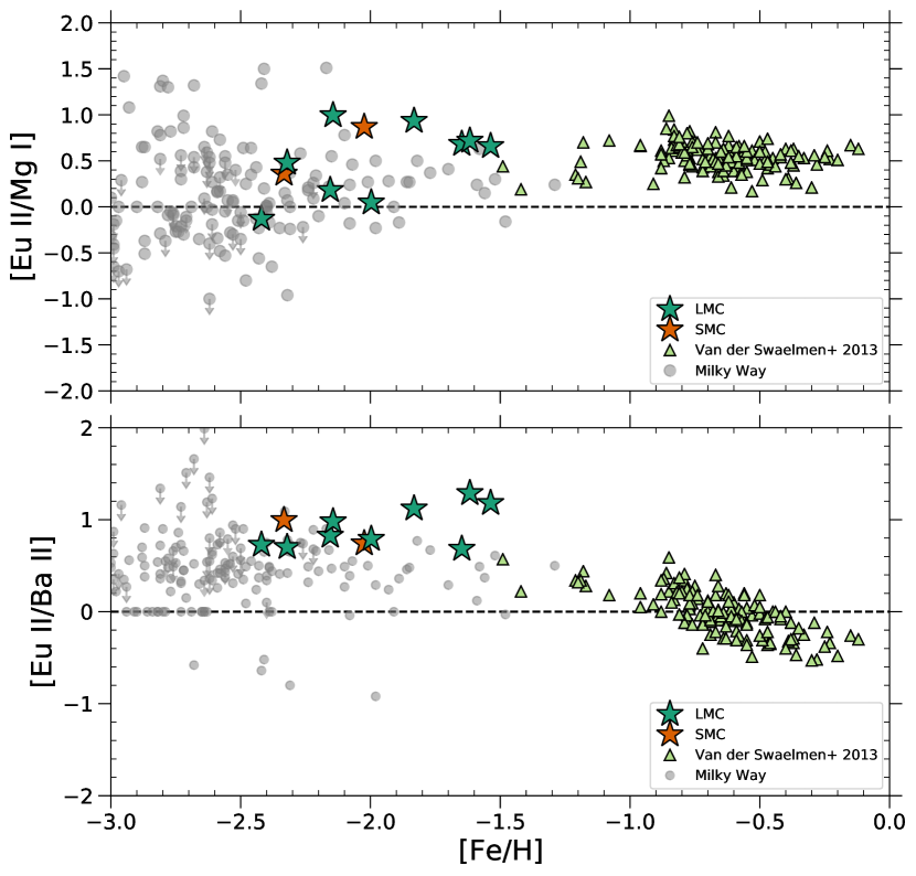
Figure 7: Magellanic Cloud $[\text{Eu/Mg}]$ and $[\text{Eu/Ba}]$ abundances as a function of metallicity. We plot as dark green stars our nine LMC giants and as orange stars our two SMC giants for which we were able to infer europium abundances. We plot as light green triangles LMC bar giants from Van der Swaelmen et al. (2013). We plot as gray circles metal-poor Milky Way giants from Barklem et al. (2005) and Jacobson et al. (2015) selected for high-resolution follow-up observations without regard to their $r$-process abundances. We find that $[\text{Eu/Mg}]$ is has no dependence on metallicity in the range $-2.6\lesssim[\text{Fe/H}]\lesssim 0$ in the Magellanic Clouds. On the other hand, $[\text{Eu/Ba}]$ declines with metallicity. The first trend is consistent with a constant ratio of the nucleosynthesis of magnesium in core-collapse supernovae and europium in compact object mergers involving a neutron star at times in excess of 100 Myr after the onset of star formation. The second trend is consistent with a constant contribution of $r$-process barium from compact object mergers involving a neutron star combined with increasing contributions with time (and therefore metallicity) of $s$-process barium from low-mass AGB stars.

We predict that future observations of galaxies that resemble the Magellanic Clouds in two key properties will also display metal-poor stellar populations with ubiquitous $r$-process enhancement. The first key property is evolution substantially in isolation that allows a galaxy to accrete unenriched gas from the cosmic web and avoid ram-pressure stripping/strangulation inside the virial radius of a more massive halo. The second key property is an intermediate mass that is high enough to be robust against stellar and supernovae feedback but low enough not to be significantly affected by AGN feedback or accretion shocks.

6 Conclusion

We observed with high-resolution Magellan/MIKE spectroscopy nine LMC and four SMC stars selected using the mid-infrared metal-poor star selection of Schlaufman & Casey (2014) and archival data. These stars are the most metal-poor Magellanic Cloud stars yet subject to a comprehensive abundance analysis. We find that in the interval $-2.6\lesssim[\text{Fe/H}]\lesssim-1.5$ these stars are similar to Milky Way halo stars in their $\alpha$, light odd-$Z$, iron-peak, and $s$-process neutron-capture element abundances, including their enhancement in $\alpha$ elements magnesium, calcium, and titanium. We discover that both the Large and Small Magellanic Clouds are ubiquitously enhanced in the $r$-process element europium relative to the Milky Way’s halo. The probabilities that the large $[\text{Eu/Fe}]$ abundances we observe in the LMC, the SMC, and our complete Magellanic Clouds sample could be explained by random sampling from an $[\text{Eu/Fe}]$ distribution like the Milky Way’s are less than 1 in 20600, 1 in 279, and 1 in $2.88\times 10^{6}$. These probabilities would be equivalent to 3.90, 2.69, and 4.96 $\sigma$ in a Gaussian distribution. Even though we studied the Magellanic Clouds’ $[\alpha/\text{Fe}]$—$[\text{Fe/H}]$ distribution to unprecedentedly low metallicities, we could not to identify a plateau in the $[\alpha/\text{Fe}]$—$[\text{Fe/H}]$ distribution and therefore were unable to identify the $[\text{Fe/H}]$ value at which $[\alpha/\text{Fe}]$ begins to decrease (i.e., the “knee”).

We argue the ubiquitous $\alpha$ and europium enhancements observed in the Magellanic Clouds are a product of their isolated chemical evolution and long history of accretion from the cosmic web that extended the era of metal-poor star formation for a much longer time in the Magellanic Clouds than in the Milky Way or M31. This extended duration of star formation allowed time for $r$-process nucleosynthesis in events that began to occur somewhere between the core-collapse supernova timescale (a few Myr after the onset of star formation) and the thermonuclear supernova timescale (a few tens to 100 Myr after the onset of star formation). These events that produced the europium enhancements we observe in the Magellanic Clouds must have been rare, otherwise $r$-process enhanced stars would be ubiquitous in the Milky Way’s ultra-faint dSphs. Compact object mergers involving a neutron star are the best candidate for a rare event that produces $r$-process nucleosynthesis on a timescale longer than the core-collapse supernova timescale. Our observations provide strong support for compact object mergers involving a neutron star occurring after core-collapse supernova but before thermonuclear supernova as the site of the $r$-process nucleosynthesis responsible for the ubiquitous europium enhancement we observe in the Magellanic Clouds in the interval $-2.6\lesssim[\text{Fe/H}]\lesssim-1.5$. We predict that metal-poor stars in intermediate-mass galaxies that evolved substantially in isolation will also be enhanced in $r$-process elements.

Table 4: Stellar Properties and Adopted Parameters

Property	J00251849-7140074	J00262394-7128549	J00263959-7122102	J00273753-7125114		Units
	SMC	SMC	SMC	SMC
Photometric Properties
SkyMapper $g$	$16.575\pm 0.036$	$17.604\pm 0.016$	$16.801\pm 0.025$	$16.987\pm 0.028$		AB mag
SkyMapper $r$	$15.917\pm 0.020$	$16.980\pm 0.014$	$16.172\pm 0.013$	$16.107\pm 0.013$		AB mag
SkyMapper $i$	$15.356\pm 0.003$	$16.403\pm 0.017$	$15.576\pm 0.040$	$15.475\pm 0.004$		AB mag
SkyMapper $z$	$15.171\pm 0.009$	$16.232\pm 0.017$	$15.407\pm 0.009$	$15.208\pm 0.003$		AB mag
2MASS $J$	$13.938\pm 0.026$	$15.076\pm 0.045$	$14.236\pm 0.030$	$14.038\pm 0.029$		Vega mag
2MASS $H$	$13.327\pm 0.035$	$14.519\pm 0.060$	$13.580\pm 0.026$	$13.351\pm 0.030$		Vega mag
2MASS $K_{\text{s}}$	$13.119\pm 0.037$	$14.295\pm 0.078$	$13.462\pm 0.051$	$13.242\pm 0.040$		Vega mag
WISE $W1$	$13.106\pm 0.024$	$14.247\pm 0.026$	$13.423\pm 0.024$	$13.092\pm 0.024$		Vega mag
WISE $W2$	$13.104\pm 0.026$	$14.268\pm 0.038$	$13.451\pm 0.028$	$13.064\pm 0.025$		Vega mag
Stellar Properties
Luminosity $L_{\ast}$	$1507^{+12}_{-22}$	$954^{+10}_{-15}$	$1387\pm 10$	$1577\pm 10$		L⊙
Radius $R_{\ast}$	$68\pm 1$	$53\pm 1$	$61\pm 1$	$71\pm 1$		R⊙
Distance $d_{\text{iso}}$	$55.0^{+0.2}_{-0.4}$	$72.1^{+0.3}_{-0.5}$	$59.6^{+0.2}_{-0.2}$	$58.3^{+0.1}_{-0.1}$		kpc
Mass $M_{\odot}$	$0.77\pm 0.01$	$0.76\pm 0.01$	$0.78\pm 0.01$	$0.76\pm 0.01$		M⊙
Age $\tau$	$13.2^{+0.2}_{-0.4}$	$13.0^{+0.3}_{-0.6}$	$13.4\pm 0.1$	$13.4\pm 0.1$		Gyr
Extinction $A_{V}$	$0.086^{+0.002}_{-0.003}$	$0.086^{+0.001}_{-0.002}$	$0.094^{+0.001}_{-0.002}$	$0.099\pm 0.001$		mag
Effective temperature $T_{\text{eff}}$	$4372^{+5}_{-3}$	$4388^{+8}_{-6}$	$4481^{+2}_{-1}$	$4326\pm 10$		K
Surface gravity $\log{g}$	$0.65\pm 0.01$	$0.87\pm 0.01$	$0.73\pm 0.01$	$0.61\pm 0.01$		cm s-2
Metallicity $[\text{Fe/H}]$	$-2.33\pm 0.30$	$-2.02\pm 0.32$	$-2.60\pm 0.39$	$-2.27\pm 0.26$
Microturbulence $\xi$	$2.71\pm 0.50$	$2.51\pm 0.80$	$3.01\pm 0.45$	$3.83\pm 0.95$		km s-1
Property	J05121686-6517147	J05133509-7109322	J05141665-6454310	J05143154-6505189	J05150380-6647003	Units
	LMC	LMC	LMC	LMC	LMC
Photometric Properties
SkyMapper $g$	$17.329\pm 0.266$	$17.367\pm 0.043$	$17.556\pm 0.021$	$17.533\pm 0.017$	$17.138\pm 0.014$	AB mag
SkyMapper $r$	$16.019\pm 0.099$	$16.682\pm 0.005$	$17.056\pm 0.007$	$16.789\pm 0.009$	$16.247\pm 0.009$	AB mag
SkyMapper $i$	$15.265\pm 0.063$	$16.178\pm 0.090$	$16.721\pm 0.043$	$16.262\pm 0.012$	$15.635\pm 0.007$	AB mag
SkyMapper $z$	$15.017\pm 0.038$	$16.009\pm 0.016$	$16.577\pm 0.017$	$16.064\pm 0.005$	$15.417\pm 0.012$	AB mag
2MASS $J$	$13.584\pm 0.030$	$14.704\pm 0.037$	$15.363\pm 0.064$	$14.847\pm 0.040$	$14.063\pm 0.030$	Vega mag
2MASS $H$	$12.751\pm 0.027$	$13.976\pm 0.051$	$14.871\pm 0.083$	$14.070\pm 0.040$	$13.233\pm 0.025$	Vega mag
2MASS $K_{\text{s}}$	$12.584\pm 0.032$	$13.896\pm 0.057$	$14.780\pm 0.125$	$14.060\pm 0.068$	$12.977\pm 0.031$	Vega mag
WISE $W1$	$12.689\pm 0.023$	$13.817\pm 0.025$	$14.691\pm 0.026$	$13.870\pm 0.024$	$\cdots$	Vega mag
WISE $W2$	$12.535\pm 0.023$	$13.915\pm 0.028$	$14.707\pm 0.034$	$14.019\pm 0.028$	$\cdots$	Vega mag
Stellar Properties
Luminosity $L_{\ast}$	$1681\pm 10$	$707^{+36}_{-24}$	$378^{+14}_{-17}$	$596\pm 10$	$1221^{+73}_{-39}$	L⊙
Radius $R_{\ast}$	$75\pm 1$	$43\pm 1$	$28\pm 1$	$42\pm 1$	$69\pm 1$	R⊙
Distance $d_{\text{iso}}$	$48.0\pm 0.1$	$49.1^{+1.3}_{-0.8}$	$50.0^{+0.9}_{-1.2}$	$51.2\pm 0.1$	$49.0^{+1.5}_{-0.8}$	kpc
Mass $M_{\odot}$	$0.75\pm 0.01$	$0.81^{+0.02}_{-0.03}$	$0.82^{+0.03}_{-0.02}$	$0.77\pm 0.01$	$0.74\pm 0.02$	M⊙
Age $\tau$	$13.3^{+0.1}_{-0.3}$	$11.3^{+1.3}_{-0.9}$	$11.9^{+1.1}_{-1.2}$	$13.4^{+0.1}_{-0.2}$	$12.3\pm 0.9$	Gyr
Extinction $A_{V}$	$0.171^{+0.004}_{-0.007}$	$0.460^{+0.024}_{-0.011}$	$0.155^{+0.007}_{-0.008}$	$0.165^{+0.001}_{-0.002}$	$0.446^{+0.012}_{-0.006}$	mag
Effective temperature $T_{\text{eff}}$	$4247\pm 1$	$4520^{+26}_{-18}$	$4761^{+18}_{-15}$	$4361^{+2}_{-1}$	$4139^{+14}_{-13}$	K
Surface gravity $\log{g}$	$0.55\pm 0.01$	$1.06\pm 0.02$	$1.43\pm 0.02$	$1.06\pm 0.01$	$0.64\pm 0.02$	cm s-2
Metallicity $[\text{Fe/H}]$	$-2.32\pm 0.36$	$-2.15\pm 0.38$	$-2.42\pm 0.23$	$-1.65\pm 0.35$	$-1.83\pm 0.46$
Microturbulence $\xi$	$2.91\pm 0.50$	$2.55\pm 0.75$	$2.45\pm 0.62$	$2.74\pm 0.83$	$3.31\pm 0.91$	km s-1
Property	J05160009-6207287	J05224088-6951471	J05242202-6945073	J06411906-7016314		Units
	LMC	LMC	LMC	LMC
Photometric Properties
SkyMapper $g$	$16.542\pm 0.008$	$17.440\pm 0.017$	$17.791\pm 0.129$	$16.776\pm 0.023$		AB mag
SkyMapper $r$	$15.770\pm 0.008$	$16.783\pm 0.029$	$17.237\pm 0.009$	$15.944\pm 0.006$		AB mag
SkyMapper $i$	$15.228\pm 0.006$	$16.418\pm 0.016$	$16.945\pm 0.011$	$15.320\pm 0.007$		AB mag
SkyMapper $z$	$14.987\pm 0.007$	$16.303\pm 0.036$	$17.020\pm 0.091$	$15.050\pm 0.004$		AB mag
2MASS $J$	$13.777\pm 0.028$	$15.026\pm 0.052$	$15.711\pm 0.080$	$13.789\pm 0.029$		Vega mag
2MASS $H$	$13.026\pm 0.024$	$14.340\pm 0.061$	$15.043\pm 0.083$	$13.015\pm 0.026$		Vega mag
2MASS $K_{\text{s}}$	$12.928\pm 0.026$	$14.368\pm 0.093$	$15.075\pm 0.158$	$12.834\pm 0.035$		Vega mag
WISE $W1$	$12.825\pm 0.023$	$14.109\pm 0.058$	$\cdots$	$12.775\pm 0.023$		Vega mag
WISE $W2$	$12.835\pm 0.022$	$14.529\pm 0.059$	$\cdots$	$12.817\pm 0.023$		Vega mag
Stellar Properties
Luminosity $L_{\ast}$	$1455^{+55}_{-54}$	$517\pm 22$	$279^{+14}_{-13}$	$1555^{+18}_{-31}$		L⊙
Radius $R_{\ast}$	$73\pm 1$	$35\pm 1$	$23\pm 1$	$78\pm 1$		R⊙
Distance $d_{\text{iso}}$	$49.6\pm 1.0$	$49.7^{+1.1}_{-1.2}$	$49.4^{+1.2}_{-1.0}$	$50.8^{+0.3}_{-0.5}$		kpc
Mass $M_{\odot}$	$0.78^{+0.03}_{-0.02}$	$0.80^{+0.03}_{-0.02}$	$0.83\pm 0.03$	$0.76^{+0.02}_{-0.01}$		M⊙
Age $\tau$	$11.6^{+1.2}_{-1.1}$	$11.9^{+1.1}_{-1.3}$	$11.5^{+1.3}_{-1.1}$	$12.8^{+0.5}_{-0.8}$		Gyr
Extinction $A_{V}$	$0.063^{+0.023}_{-0.028}$	$0.271^{+0.058}_{-0.039}$	$0.038^{+0.048}_{-0.026}$	$0.220^{+0.004}_{-0.006}$		mag
Effective temperature $T_{\text{eff}}$	$4151\pm 17$	$4619^{+45}_{-23}$	$4903^{+31}_{-49}$	$4093^{+8}_{-7}$		K
Surface gravity $\log{g}$	$0.60\pm 0.02$	$1.24\pm 0.03$	$1.61\pm 0.03$	$0.53\pm 0.01$		cm s-2
Metallicity $[\text{Fe/H}]$	$-1.62\pm 0.24$	$-2.14\pm 0.32$	$-1.99\pm 0.47$	$-1.54\pm 0.14$
Microturbulence $\xi$	$3.25\pm 0.54$	$3.16\pm 0.45$	$2.38\pm 0.78$	$3.28\pm 0.47$		km s-1

Table 5: Mean Elemental Abundances

Species	n	log($\epsilon_{X}$)	[X/Fe]	$\sigma_{[\text{X/Fe}]}$	n	log($\epsilon_{X}$)	[X/Fe]	$\sigma_{[\text{X/Fe}]}$	n	log($\epsilon_{X}$)	[X/Fe]	$\sigma_{[\text{X/Fe}]}$	n	log($\epsilon_{X}$)	[X/Fe]	$\sigma_{[\text{X/Fe}]}$	n	log($\epsilon_{X}$)	[X/Fe]	$\sigma_{[\text{X/Fe}]}$
	J00251849-7140074				J00262394-7128549				J00263959-7122102				J00273753-7125114				J05121686-6517147
	SMC				SMC				SMC				SMC				LMC
Na I	$2$	$4.187$	$0.300$	$0.264$	$3$	$3.974$	$-0.222$	$0.210$	$2$	$4.168$	$0.550$	$0.264$	$2$	$3.447$	$-0.508$	$0.254$	$1$	$4.166$	$0.267$	$0.100$
Na INLTE	$2$	$4.072$	$0.166$	$\cdots$	$3$	$3.877$	$-0.339$	$\cdots$	$2$	$3.916$	$0.278$	$\cdots$	$2$	$3.329$	$-0.646$	$\cdots$	$1$	$4.123$	$0.204$	$\cdots$
Mg I	$2$	$5.710$	$0.493$	$0.287$	$2$	$5.662$	$0.136$	$0.211$	$1$	$5.523$	$0.575$	$0.123$	$2$	$5.651$	$0.366$	$0.090$	$2$	$6.300$	$1.071$	$0.236$
Si I	$3$	$5.864$	$0.687$	$0.174$	$4$	$6.027$	$0.541$	$0.023$	$4$	$6.204$	$1.296$	$0.090$	$2$	$5.757$	$0.512$	$0.029$	$2$	$5.835$	$0.646$	$0.216$
K I	$1$	$3.569$	$0.832$	$0.192$	$1$	$3.237$	$0.191$	$0.151$	$1$	$3.679$	$1.211$	$0.174$	$1$	$3.224$	$0.419$	$0.099$	$1$	$4.793$	$2.044$	$0.356$
K INLTE	$1$	$2.854$	$0.157$	$\cdots$	$1$	$2.932$	$-0.074$	$\cdots$	$1$	$2.938$	$0.510$	$\cdots$	$1$	$2.711$	$-0.054$	$\cdots$	$1$	$3.580$	$0.871$	$\cdots$
Ca I	$14$	$4.581$	$0.614$	$0.132$	$9$	$4.383$	$0.107$	$0.150$	$8$	$4.547$	$0.849$	$0.096$	$12$	$4.429$	$0.394$	$0.083$	$11$	$4.958$	$0.979$	$0.298$
Sc II	$5$	$0.736$	$-0.071$	$0.079$	$4$	$0.870$	$-0.246$	$0.138$	$4$	$0.899$	$0.361$	$0.069$	$4$	$0.989$	$0.114$	$0.072$	$3$	$1.257$	$0.438$	$0.225$
Ti I	$13$	$3.265$	$0.628$	$0.164$	$9$	$3.199$	$0.253$	$0.165$	$10$	$3.363$	$0.995$	$0.176$	$12$	$3.184$	$0.479$	$0.115$	$48$	$4.364$	$1.715$	$0.371$
Ti II	$5$	$3.307$	$0.670$	$0.125$	$6$	$3.313$	$0.367$	$0.203$	$5$	$3.178$	$0.810$	$0.169$	$6$	$2.878$	$0.173$	$0.106$	$38$	$3.322$	$0.673$	$0.176$
Cr I	$6$	$3.632$	$0.345$	$0.289$	$5$	$3.262$	$-0.334$	$0.241$	$2$	$3.178$	$0.160$	$0.141$	$5$	$3.419$	$0.064$	$0.228$	$4$	$3.150$	$-0.149$	$0.363$
Mn I	$2$	$3.032$	$-0.055$	$0.143$	$4$	$2.809$	$-0.587$	$0.212$	$3$	$2.865$	$0.047$	$0.144$	$3$	$2.778$	$-0.377$	$0.129$	$2$	$2.546$	$-0.553$	$0.710$
Fe I	$31$	$5.294$	$\cdots$	$\cdots$	$26$	$5.222$	$\cdots$	$\cdots$	$27$	$5.190$	$\cdots$	$\cdots$	$23$	$4.998$	$\cdots$	$\cdots$	$28$	$5.478$	$\cdots$	$\cdots$
Fe II	$24$	$5.163$	$\cdots$	$\cdots$	$20$	$5.464$	$\cdots$	$\cdots$	$14$	$4.898$	$\cdots$	$\cdots$	$12$	$5.229$	$\cdots$	$\cdots$	$18$	$5.175$	$\cdots$	$\cdots$
Co I	$3$	$3.321$	$0.714$	$0.214$	$2$	$3.081$	$0.165$	$0.214$	$2$	$2.920$	$0.582$	$0.162$	$1$	$2.822$	$0.147$	$0.041$	$5$	$3.391$	$0.772$	$0.201$
Ni I	$14$	$4.172$	$0.305$	$0.144$	$7$	$3.882$	$-0.294$	$0.117$	$9$	$4.043$	$0.445$	$0.119$	$7$	$3.911$	$-0.024$	$0.134$	$7$	$4.360$	$0.481$	$0.261$
Cu I	$1$	$2.073$	$0.226$	$0.144$	$\cdots$	$\cdots$	$\cdots$	$\cdots$	$\cdots$	$\cdots$	$\cdots$	$\cdots$	$1$	$1.785$	$-0.130$	$0.068$	$1$	$3.255$	$1.396$	$0.413$
Zn I	$\cdots$	$\cdots$	$\cdots$	$\cdots$	$\cdots$	$\cdots$	$\cdots$	$\cdots$	$\cdots$	$\cdots$	$\cdots$	$\cdots$	$\cdots$	$\cdots$	$\cdots$	$\cdots$	$1$	$2.772$	$0.533$	$0.121$
Y II	$2$	$-0.215$	$-0.092$	$0.205$	$3$	$0.599$	$0.413$	$0.404$	$3$	$0.221$	$0.613$	$0.182$	$3$	$0.257$	$0.312$	$0.377$	$2$	$-0.105$	$0.006$	$0.123$
Ba II	$3$	$-0.205$	$-0.142$	$0.264$	$2$	$0.508$	$0.262$	$0.292$	$3$	$-0.428$	$-0.096$	$0.201$	$3$	$-0.461$	$-0.466$	$0.161$	$3$	$0.798$	$0.849$	$0.292$
La II	$\cdots$	$\cdots$	$\cdots$	$\cdots$	$\cdots$	$\cdots$	$\cdots$	$\cdots$	$\cdots$	$\cdots$	$\cdots$	$\cdots$	$\cdots$	$\cdots$	$\cdots$	$\cdots$	$3$	$0.153$	$1.364$	$0.278$
Ce II	$2$	$-0.664$	$0.089$	$0.062$	$3$	$1.305$	$1.749$	$1.619$	$2$	$-0.355$	$0.667$	$0.280$	$2$	$-0.545$	$0.140$	$0.282$	$3$	$-0.118$	$0.623$	$0.588$
Nd II	$2$	$-1.009$	$-0.096$	$0.188$	$5$	$-0.166$	$0.438$	$0.196$	$3$	$-0.602$	$0.580$	$0.198$	$\cdots$	$\cdots$	$\cdots$	$\cdots$	$5$	$0.370$	$1.271$	$0.434$
Sm II	$1$	$-0.865$	$0.518$	$0.056$	$2$	$-0.409$	$0.665$	$0.275$	$\cdots$	$\cdots$	$\cdots$	$\cdots$	$\cdots$	$\cdots$	$\cdots$	$\cdots$	$1$	$-0.900$	$0.471$	$0.043$
Gd II	$1$	$0.005$	$1.258$	$0.133$	$2$	$-0.132$	$0.812$	$0.266$	$1$	$-0.382$	$1.140$	$0.045$	$\cdots$	$\cdots$	$\cdots$	$\cdots$	$2$	$-0.579$	$0.662$	$0.122$
Eu II	$1$	$-0.960$	$0.853$	$0.300$	$1$	$-0.500$	$1.004$	$0.300$	$\cdots$	$\cdots$	$\cdots$	$\cdots$	$\cdots$	$\cdots$	$\cdots$	$\cdots$	$1$	$-0.250$	$1.551$	$0.300$
	J05133509-7109322				J05141665-6454310				J05143154-6505189				J05150380-6647003				J05160009-6207287
	LMC				LMC				LMC				LMC				LMC
Na I	$3$	$4.209$	$0.144$	$0.167$	$2$	$4.111$	$0.311$	$0.141$	$2$	$5.308$	$0.736$	$0.276$	$2$	$5.406$	$1.018$	$0.272$	$2$	$4.826$	$0.223$	$0.122$
Na INLTE	$3$	$4.100$	$0.015$	$\cdots$	$2$	$4.053$	$0.234$	$\cdots$	$2$	$5.159$	$0.567$	$\cdots$	$2$	$5.237$	$0.830$	$\cdots$	$2$	$4.755$	$0.133$	$\cdots$
Mg I	$4$	$5.868$	$0.473$	$0.230$	$6$	$5.660$	$0.530$	$0.136$	$3$	$6.116$	$0.214$	$0.419$	$1$	$5.836$	$0.118$	$0.229$	$6$	$5.862$	$-0.071$	$0.302$
Si I	$4$	$6.187$	$0.832$	$0.081$	$4$	$5.993$	$0.903$	$0.092$	$4$	$6.834$	$0.972$	$0.100$	$5$	$6.361$	$0.683$	$0.079$	$7$	$6.575$	$0.682$	$0.094$
K I	$1$	$3.338$	$0.423$	$0.200$	$1$	$5.854$	$3.204$	$0.194$	$1$	$4.358$	$0.936$	$0.325$	$1$	$3.886$	$0.648$	$0.300$	$1$	$3.482$	$0.029$	$0.205$
K INLTE	$1$	$3.010$	$0.135$	$\cdots$	$1$	$3.850$	$1.240$	$\cdots$	$1$	$3.960$	$0.578$	$\cdots$	$1$	$2.979$	$-0.219$	$\cdots$	$1$	$2.578$	$-0.835$	$\cdots$
Ca I	$16$	$4.615$	$0.470$	$0.204$	$17$	$4.253$	$0.373$	$0.136$	$7$	$5.342$	$0.690$	$0.321$	$6$	$5.054$	$0.586$	$0.258$	$17$	$4.620$	$-0.063$	$0.223$
Sc II	$5$	$1.136$	$0.151$	$0.127$	$3$	$0.746$	$0.026$	$0.141$	$5$	$1.654$	$0.162$	$0.210$	$5$	$1.431$	$0.123$	$0.213$	$5$	$1.534$	$0.011$	$0.177$
Ti I	$43$	$3.253$	$0.438$	$0.228$	$35$	$3.031$	$0.481$	$0.139$	$24$	$3.729$	$0.407$	$0.269$	$19$	$3.709$	$0.571$	$0.271$	$35$	$3.433$	$0.080$	$0.183$
Ti II	$35$	$3.243$	$0.428$	$0.167$	$44$	$2.887$	$0.337$	$0.120$	$23$	$3.563$	$0.241$	$0.186$	$26$	$3.435$	$0.297$	$0.146$	$35$	$3.619$	$0.266$	$0.184$
Cr I	$13$	$3.589$	$0.124$	$0.279$	$10$	$3.193$	$-0.007$	$0.151$	$5$	$4.129$	$0.157$	$0.399$	$3$	$3.677$	$-0.111$	$0.359$	$15$	$3.602$	$-0.401$	$0.309$
Mn I	$5$	$2.965$	$-0.300$	$0.244$	$5$	$2.689$	$-0.311$	$0.157$	$3$	$2.912$	$-0.860$	$0.461$	$3$	$3.428$	$-0.160$	$0.239$	$6$	$3.570$	$-0.233$	$0.116$
Fe I	$79$	$5.222$	$\cdots$	$\cdots$	$88$	$5.094$	$\cdots$	$\cdots$	$36$	$5.398$	$\cdots$	$\cdots$	$29$	$5.466$	$\cdots$	$\cdots$	$37$	$5.354$	$\cdots$	$\cdots$
Fe II	$28$	$5.340$	$\cdots$	$\cdots$	$26$	$5.076$	$\cdots$	$\cdots$	$24$	$5.841$	$\cdots$	$\cdots$	$23$	$5.658$	$\cdots$	$\cdots$	$26$	$5.877$	$\cdots$	$\cdots$
Co I	$5$	$3.216$	$0.431$	$0.223$	$4$	$3.157$	$0.637$	$0.342$	$5$	$3.985$	$0.693$	$0.128$	$4$	$3.715$	$0.607$	$0.190$	$6$	$3.574$	$0.251$	$0.049$
Ni I	$16$	$4.105$	$0.060$	$0.177$	$6$	$3.851$	$0.071$	$0.173$	$12$	$4.678$	$0.126$	$0.240$	$19$	$4.533$	$0.165$	$0.164$	$22$	$4.367$	$-0.216$	$0.151$
Cu I	$1$	$2.348$	$0.323$	$0.247$	$\cdots$	$\cdots$	$\cdots$	$\cdots$	$1$	$1.819$	$-0.713$	$0.154$	$1$	$4.115$	$1.767$	$0.421$	$1$	$1.906$	$-0.657$	$0.141$
Zn I	$2$	$2.591$	$0.186$	$0.064$	$2$	$2.498$	$0.358$	$0.144$	$2$	$3.022$	$0.110$	$0.161$	$2$	$3.030$	$0.302$	$0.140$	$2$	$2.982$	$0.039$	$0.276$
Y II	$4$	$-0.168$	$-0.223$	$0.135$	$5$	$-0.010$	$0.200$	$0.287$	$3$	$-0.026$	$-0.588$	$0.135$	$4$	$0.713$	$0.335$	$0.367$	$3$	$0.640$	$0.047$	$0.208$
Ba II	$3$	$-0.055$	$-0.170$	$0.342$	$3$	$-0.477$	$-0.327$	$0.170$	$3$	$0.837$	$0.215$	$0.323$	$3$	$0.369$	$-0.069$	$0.297$	$3$	$0.012$	$-0.641$	$0.258$
La II	$2$	$-1.020$	$0.025$	$0.252$	$3$	$-0.532$	$0.778$	$0.141$	$3$	$0.059$	$0.597$	$0.314$	$3$	$-0.121$	$0.601$	$0.248$	$2$	$-0.290$	$0.217$	$0.202$
Ce II	$5$	$-0.602$	$-0.027$	$0.287$	$2$	$-0.706$	$0.134$	$0.308$	$4$	$0.148$	$0.216$	$0.258$	$3$	$-0.392$	$-0.140$	$0.352$	$2$	$0.053$	$0.090$	$0.133$
Nd II	$6$	$-0.491$	$0.244$	$0.133$	$5$	$-0.828$	$0.172$	$0.138$	$5$	$0.077$	$0.305$	$0.198$	$6$	$0.079$	$0.491$	$0.322$	$3$	$0.014$	$0.211$	$0.138$
Sm II	$1$	$-0.449$	$0.756$	$0.090$	$1$	$-1.124$	$0.346$	$0.062$	$1$	$0.316$	$1.014$	$0.204$	$1$	$-0.076$	$0.806$	$0.112$	$2$	$-0.135$	$0.532$	$0.277$
Gd II	$2$	$-0.562$	$0.513$	$0.157$	$3$	$-0.363$	$0.977$	$0.249$	$2$	$-0.043$	$0.525$	$0.162$	$1$	$-0.040$	$0.712$	$0.087$	$2$	$0.451$	$0.988$	$0.277$
Eu II	$1$	$-0.980$	$0.655$	$0.150$	$2$	$-1.500$	$0.400$	$0.300$	$1$	$-0.230$	$0.898$	$0.300$	$1$	$-0.260$	$1.052$	$0.150$	$1$	$-0.450$	$0.647$	$0.200$
	J05224088-6951471				J05242202-6945073				J06411906-7016314
	LMC				LMC				LMC
Na I	$2$	$3.922$	$-0.154$	$0.317$	$2$	$4.172$	$-0.051$	$0.406$	$2$	$4.290$	$-0.393$	$0.151$
Na INLTE	$2$	$3.383$	$-0.670$	$\cdots$	$2$	$3.664$	$-0.560$	$\cdots$	$2$	$4.275$	$-0.428$	$\cdots$
Mg I	$6$	$5.625$	$0.219$	$0.164$	$4$	$5.993$	$0.440$	$0.185$	$4$	$5.850$	$-0.163$	$0.244$
Si I	$4$	$5.748$	$0.382$	$0.080$	$6$	$5.902$	$0.389$	$0.088$	$6$	$6.153$	$0.180$	$0.114$
K I	$1$	$2.638$	$-0.430$	$0.123$	$1$	$5.660$	$1.257$	$0.221$	$1$	$3.325$	$-0.208$	$0.165$
K INLTE	$1$	$2.490$	$-0.236$	$\cdots$	$1$	$4.330$	$0.776$	$\cdots$	$1$	$3.111$	$-0.382$	$\cdots$
Ca I	$19$	$4.337$	$0.181$	$0.129$	$19$	$4.576$	$0.273$	$0.135$	$19$	$4.535$	$-0.228$	$0.180$
Sc II	$5$	$1.025$	$0.029$	$0.124$	$5$	$1.142$	$-0.001$	$0.121$	$5$	$1.531$	$-0.072$	$0.168$
Ti I	$38$	$3.251$	$0.425$	$0.176$	$27$	$3.531$	$0.558$	$0.159$	$36$	$3.160$	$-0.273$	$0.140$
Ti II	$33$	$3.035$	$0.209$	$0.105$	$33$	$3.171$	$0.198$	$0.149$	$42$	$3.552$	$0.119$	$0.181$
Cr I	$14$	$3.331$	$-0.145$	$0.183$	$11$	$3.614$	$-0.009$	$0.187$	$14$	$3.477$	$-0.606$	$0.250$
Mn I	$5$	$3.082$	$-0.194$	$0.184$	$4$	$2.657$	$-0.766$	$0.130$	$5$	$3.291$	$-0.592$	$0.051$
Fe I	$81$	$5.119$	$\cdots$	$\cdots$	$78$	$5.430$	$\cdots$	$\cdots$	$34$	$5.451$	$\cdots$	$\cdots$
Fe II	$26$	$5.306$	$\cdots$	$\cdots$	$26$	$5.453$	$\cdots$	$\cdots$	$25$	$5.954$	$\cdots$	$\cdots$
Co I	$3$	$3.158$	$0.362$	$0.195$	$3$	$3.401$	$0.458$	$0.147$	$5$	$3.278$	$-0.125$	$0.070$
Ni I	$15$	$4.073$	$0.017$	$0.160$	$11$	$4.452$	$0.249$	$0.203$	$22$	$4.329$	$-0.334$	$0.123$
Cu I	$\cdots$	$\cdots$	$\cdots$	$\cdots$	$\cdots$	$\cdots$	$\cdots$	$\cdots$	$1$	$1.975$	$-0.668$	$0.138$
Zn I	$2$	$2.569$	$0.153$	$0.143$	$2$	$2.730$	$0.167$	$0.131$	$2$	$2.671$	$-0.352$	$0.094$
Y II	$5$	$0.229$	$0.163$	$0.117$	$2$	$0.207$	$-0.006$	$0.177$	$3$	$0.285$	$-0.388$	$0.122$
Ba II	$3$	$0.359$	$0.233$	$0.251$	$3$	$-0.031$	$-0.304$	$0.220$	$3$	$0.049$	$-0.684$	$0.236$
La II	$3$	$0.113$	$1.147$	$0.100$	$3$	$-0.412$	$0.475$	$0.216$	$2$	$-0.478$	$-0.051$	$0.216$
Ce II	$5$	$-0.106$	$0.458$	$0.227$	$2$	$0.433$	$0.850$	$0.256$	$2$	$0.084$	$0.041$	$0.143$
Nd II	$6$	$0.419$	$1.143$	$0.246$	$5$	$-0.052$	$0.525$	$0.147$	$3$	$0.198$	$0.315$	$0.135$
Sm II	$2$	$0.055$	$1.249$	$0.162$	$2$	$-0.421$	$0.626$	$0.125$	$2$	$-0.394$	$0.193$	$0.099$
Gd II	$3$	$0.394$	$1.458$	$0.202$	$1$	$-0.106$	$0.811$	$0.093$	$1$	$0.044$	$0.501$	$0.094$
Eu II	$1$	$-0.410$	$1.214$	$0.150$	$1$	$-0.990$	$0.487$	$0.300$	$1$	$-0.520$	$0.497$	$0.200$

References

- Ahumada et al. (2020) Ahumada, R., Prieto, C. A., Almeida, A., et al. 2020, ApJS, 249, 3, doi: 10.3847/1538-4365/ab929e
- Amarsi & Asplund (2017) Amarsi, A. M., & Asplund, M. 2017, MNRAS, 464, 264, doi: 10.1093/mnras/stw2445
- Amarsi et al. (2016) Amarsi, A. M., Lind, K., Asplund, M., Barklem, P. S., & Collet, R. 2016, MNRAS, 463, 1518, doi: 10.1093/mnras/stw2077
- Amarsi et al. (2020) Amarsi, A. M., Lind, K., Osorio, Y., et al. 2020, A&A, 642, A62, doi: 10.1051/0004-6361/202038650
- Arenou et al. (2018) Arenou, F., Luri, X., Babusiaux, C., et al. 2018, A&A, 616, A17, doi: 10.1051/0004-6361/201833234
- Astropy Collaboration et al. (2013) Astropy Collaboration, Robitaille, T. P., Tollerud, E. J., et al. 2013, A&A, 558, A33, doi: 10.1051/0004-6361/201322068
- Astropy Collaboration et al. (2018) Astropy Collaboration, Price-Whelan, A. M., Sipőcz, B. M., et al. 2018, AJ, 156, 123, doi: 10.3847/1538-3881/aabc4f
- Baldry et al. (2004) Baldry, I. K., Glazebrook, K., Brinkmann, J., et al. 2004, ApJ, 600, 681, doi: 10.1086/380092
- Barklem et al. (2005) Barklem, P. S., Christlieb, N., Beers, T. C., et al. 2005, A&A, 439, 129, doi: 10.1051/0004-6361:20052967
- Bartos & Marka (2019) Bartos, I., & Marka, S. 2019, Nature, 569, 85, doi: 10.1038/s41586-019-1113-7
- Beers & Christlieb (2005) Beers, T. C., & Christlieb, N. 2005, ARA&A, 43, 531, doi: 10.1146/annurev.astro.42.053102.134057
- Bekki & Stanimirović (2009) Bekki, K., & Stanimirović, S. 2009, MNRAS, 395, 342, doi: 10.1111/j.1365-2966.2009.14514.x
- Bekki & Tsujimoto (2012) Bekki, K., & Tsujimoto, T. 2012, ApJ, 761, 180, doi: 10.1088/0004-637X/761/2/180
- Benson et al. (2002a) Benson, A. J., Frenk, C. S., Lacey, C. G., Baugh, C. M., & Cole, S. 2002a, MNRAS, 333, 177, doi: 10.1046/j.1365-8711.2002.05388.x
- Benson et al. (2002b) Benson, A. J., Lacey, C. G., Baugh, C. M., Cole, S., & Frenk, C. S. 2002b, MNRAS, 333, 156, doi: 10.1046/j.1365-8711.2002.05387.x
- Bergemann (2011) Bergemann, M. 2011, MNRAS, 413, 2184, doi: 10.1111/j.1365-2966.2011.18295.x
- Bergemann & Cescutti (2010) Bergemann, M., & Cescutti, G. 2010, A&A, 522, A9, doi: 10.1051/0004-6361/201014250
- Bernstein et al. (2003) Bernstein, R., Shectman, S. A., Gunnels, S. M., Mochnacki, S., & Athey, A. E. 2003, in Society of Photo-Optical Instrumentation Engineers (SPIE) Conference Series, Vol. 4841, Proc. SPIE, ed. M. Iye & A. F. M. Moorwood, 1694–1704, doi: 10.1117/12.461502
- Besla et al. (2007) Besla, G., Kallivayalil, N., Hernquist, L., et al. 2007, ApJ, 668, 949, doi: 10.1086/521385
- Besla et al. (2010) —. 2010, ApJ, 721, L97, doi: 10.1088/2041-8205/721/2/L97
- Birnboim & Dekel (2003) Birnboim, Y., & Dekel, A. 2003, MNRAS, 345, 349, doi: 10.1046/j.1365-8711.2003.06955.x
- Blanco-Cuaresma (2019) Blanco-Cuaresma, S. 2019, MNRAS, 486, 2075, doi: 10.1093/mnras/stz549
- Blanco-Cuaresma et al. (2014) Blanco-Cuaresma, S., Soubiran, C., Heiter, U., & Jofré, P. 2014, A&A, 569, A111, doi: 10.1051/0004-6361/201423945
- Bland-Hawthorn et al. (2015) Bland-Hawthorn, J., Sutherland, R., & Webster, D. 2015, ApJ, 807, 154, doi: 10.1088/0004-637X/807/2/154
- Blanton et al. (2003) Blanton, M. R., Hogg, D. W., Bahcall, N. A., et al. 2003, ApJ, 594, 186, doi: 10.1086/375528
- Blanton et al. (2017) Blanton, M. R., Bershady, M. A., Abolfathi, B., et al. 2017, AJ, 154, 28, doi: 10.3847/1538-3881/aa7567
- Boch & Fernique (2014) Boch, T., & Fernique, P. 2014, in Astronomical Society of the Pacific Conference Series, Vol. 485, Astronomical Data Analysis Software and Systems XXIII, ed. N. Manset & P. Forshay, 277
- Bonnarel et al. (2000) Bonnarel, F., Fernique, P., Bienaymé, O., et al. 2000, A&AS, 143, 33, doi: 10.1051/aas:2000331
- Brown et al. (2012) Brown, T. M., Tumlinson, J., Geha, M., et al. 2012, ApJ, 753, L21, doi: 10.1088/2041-8205/753/1/L21
- Brown et al. (2014) —. 2014, ApJ, 796, 91, doi: 10.1088/0004-637X/796/2/91
- Bullock et al. (2000) Bullock, J. S., Kravtsov, A. V., & Weinberg, D. H. 2000, ApJ, 539, 517, doi: 10.1086/309279
- Carrera et al. (2008) Carrera, R., Gallart, C., Hardy, E., Aparicio, A., & Zinn, R. 2008, AJ, 135, 836, doi: 10.1088/0004-6256/135/3/836
- Casey & Schlaufman (2017) Casey, A. R., & Schlaufman, K. C. 2017, ApJ, 850, 179, doi: 10.3847/1538-4357/aa9079
- Castelli & Kurucz (2004) Castelli, F., & Kurucz, R. L. 2004, arXiv Astrophysics e-prints
- Cayrel et al. (2004) Cayrel, R., Depagne, E., Spite, M., et al. 2004, A&A, 416, 1117, doi: 10.1051/0004-6361:20034074
- Cescutti et al. (2006) Cescutti, G., François, P., Matteucci, F., Cayrel, R., & Spite, M. 2006, A&A, 448, 557, doi: 10.1051/0004-6361:20053622
- Choi et al. (2016) Choi, J., Dotter, A., Conroy, C., et al. 2016, ApJ, 823, 102, doi: 10.3847/0004-637X/823/2/102
- Clayton (2007) Clayton, D. 2007, Handbook of Isotopes in the Cosmos
- Cole et al. (2005) Cole, A. A., Tolstoy, E., Gallagher, John S., I., & Smecker-Hane, T. A. 2005, AJ, 129, 1465, doi: 10.1086/428007
- Da Costa & Hatzidimitriou (1998) Da Costa, G. S., & Hatzidimitriou, D. 1998, AJ, 115, 1934, doi: 10.1086/300340
- Dekel & Birnboim (2006) Dekel, A., & Birnboim, Y. 2006, MNRAS, 368, 2, doi: 10.1111/j.1365-2966.2006.10145.x
- Di Teodoro et al. (2019) Di Teodoro, E. M., McClure-Griffiths, N. M., Jameson, K. E., et al. 2019, MNRAS, 483, 392, doi: 10.1093/mnras/sty3095
- Dobbie et al. (2014) Dobbie, P. D., Cole, A. A., Subramaniam, A., & Keller, S. 2014, MNRAS, 442, 1680, doi: 10.1093/mnras/stu926
- Dotter (2016) Dotter, A. 2016, ApJS, 222, 8, doi: 10.3847/0067-0049/222/1/8
- Erkal et al. (2019) Erkal, D., Belokurov, V., Laporte, C. F. P., et al. 2019, MNRAS, 487, 2685, doi: 10.1093/mnras/stz1371
- Escala et al. (2020a) Escala, I., Gilbert, K. M., Kirby, E. N., et al. 2020a, ApJ, 889, 177, doi: 10.3847/1538-4357/ab6659
- Escala et al. (2019) Escala, I., Kirby, E. N., Gilbert, K. M., Cunningham, E. C., & Wojno, J. 2019, ApJ, 878, 42, doi: 10.3847/1538-4357/ab1eac
- Escala et al. (2020b) Escala, I., Kirby, E. N., Gilbert, K. M., et al. 2020b, ApJ, 902, 51, doi: 10.3847/1538-4357/abb474
- Ezzeddine et al. (2020) Ezzeddine, R., Rasmussen, K., Frebel, A., et al. 2020, ApJ, 898, 150, doi: 10.3847/1538-4357/ab9d1a
- Fabian (2012) Fabian, A. C. 2012, ARA&A, 50, 455, doi: 10.1146/annurev-astro-081811-125521
- Feroz & Hobson (2008) Feroz, F., & Hobson, M. P. 2008, MNRAS, 384, 449, doi: 10.1111/j.1365-2966.2007.12353.x
- Feroz et al. (2009) Feroz, F., Hobson, M. P., & Bridges, M. 2009, MNRAS, 398, 1601, doi: 10.1111/j.1365-2966.2009.14548.x
- Feroz et al. (2019) Feroz, F., Hobson, M. P., Cameron, E., & Pettitt, A. N. 2019, The Open Journal of Astrophysics, 2, 10, doi: 10.21105/astro.1306.2144
- Frebel et al. (2013) Frebel, A., Casey, A. R., Jacobson, H. R., & Yu, Q. 2013, ApJ, 769, 57, doi: 10.1088/0004-637X/769/1/57
- Frebel & Norris (2015) Frebel, A., & Norris, J. E. 2015, ARA&A, 53, 631, doi: 10.1146/annurev-astro-082214-122423
- Fritz et al. (2018) Fritz, T. K., Battaglia, G., Pawlowski, M. S., et al. 2018, A&A, 619, A103, doi: 10.1051/0004-6361/201833343
- Fryer et al. (2006) Fryer, C. L., Herwig, F., Hungerford, A., & Timmes, F. X. 2006, ApJ, 646, L131, doi: 10.1086/507071
- Gaia Collaboration et al. (2016) Gaia Collaboration, Prusti, T., de Bruijne, J. H. J., et al. 2016, A&A, 595, A1, doi: 10.1051/0004-6361/201629272
- Gaia Collaboration et al. (2018) Gaia Collaboration, Helmi, A., van Leeuwen, F., et al. 2018, A&A, 616, A12, doi: 10.1051/0004-6361/201832698
- García Pérez et al. (2016) García Pérez, A. E., Allende Prieto, C., Holtzman, J. A., et al. 2016, AJ, 151, 144, doi: 10.3847/0004-6256/151/6/144
- Geha et al. (2012) Geha, M., Blanton, M. R., Yan, R., & Tinker, J. L. 2012, ApJ, 757, 85, doi: 10.1088/0004-637X/757/1/85
- Gilbert et al. (2020) Gilbert, K. M., Wojno, J., Kirby, E. N., et al. 2020, AJ, 160, 41, doi: 10.3847/1538-3881/ab9602
- Glatt et al. (2008) Glatt, K., Gallagher, John S., I., Grebel, E. K., et al. 2008, AJ, 135, 1106, doi: 10.1088/0004-6256/135/4/1106
- Graczyk et al. (2014) Graczyk, D., Pietrzyński, G., Thompson, I. B., et al. 2014, ApJ, 780, 59, doi: 10.1088/0004-637X/780/1/59
- Grunblatt et al. (2021) Grunblatt, S. K., Zinn, J. C., Price-Whelan, A. M., et al. 2021, arXiv e-prints, arXiv:2105.10505. https://arxiv.org/abs/2105.10505
- Gunn & Gott (1972) Gunn, J. E., & Gott, J. Richard, I. 1972, ApJ, 176, 1, doi: 10.1086/151605
- Hansen et al. (2017) Hansen, T. T., Simon, J. D., Marshall, J. L., et al. 2017, ApJ, 838, 44, doi: 10.3847/1538-4357/aa634a
- Hansen et al. (2018) Hansen, T. T., Holmbeck, E. M., Beers, T. C., et al. 2018, ApJ, 858, 92, doi: 10.3847/1538-4357/aabacc
- Harris & Zaritsky (2004) Harris, J., & Zaritsky, D. 2004, AJ, 127, 1531, doi: 10.1086/381953
- Harris & Zaritsky (2009) —. 2009, AJ, 138, 1243, doi: 10.1088/0004-6256/138/5/1243
- Heger & Woosley (2010) Heger, A., & Woosley, S. E. 2010, ApJ, 724, 341, doi: 10.1088/0004-637X/724/1/341
- Holmbeck et al. (2020) Holmbeck, E. M., Hansen, T. T., Beers, T. C., et al. 2020, ApJS, 249, 30, doi: 10.3847/1538-4365/ab9c19
- Hotokezaka et al. (2015) Hotokezaka, K., Piran, T., & Paul, M. 2015, Nature Physics, 11, 1042, doi: 10.1038/nphys3574
- Jacobson & Friel (2013) Jacobson, H. R., & Friel, E. D. 2013, AJ, 145, 107, doi: 10.1088/0004-6256/145/4/107
- Jacobson et al. (2015) Jacobson, H. R., Keller, S., Frebel, A., et al. 2015, ApJ, 807, 171, doi: 10.1088/0004-637X/807/2/171
- Jahn et al. (2019) Jahn, E. D., Sales, L. V., Wetzel, A., et al. 2019, MNRAS, 489, 5348, doi: 10.1093/mnras/stz2457
- Ji et al. (2016a) Ji, A. P., Frebel, A., Chiti, A., & Simon, J. D. 2016a, Nature, 531, 610, doi: 10.1038/nature17425
- Ji et al. (2016b) Ji, A. P., Frebel, A., Simon, J. D., & Chiti, A. 2016b, ApJ, 830, 93, doi: 10.3847/0004-637X/830/2/93
- Ji et al. (2020) Ji, A. P., Li, T. S., Hansen, T. T., et al. 2020, AJ, 160, 181, doi: 10.3847/1538-3881/abacb6
- Johnson et al. (2004) Johnson, J. A., Bolte, M., Hesser, J. E., Ivans, I. I., & Stetson, P. B. 2004, in Origin and Evolution of the Elements, ed. A. McWilliam & M. Rauch, 29
- Kafle et al. (2018) Kafle, P. R., Sharma, S., Lewis, G. F., Robotham, A. S. G., & Driver, S. P. 2018, MNRAS, 475, 4043, doi: 10.1093/mnras/sty082
- Kallivayalil et al. (2013) Kallivayalil, N., van der Marel, R. P., Besla, G., Anderson, J., & Alcock, C. 2013, ApJ, 764, 161, doi: 10.1088/0004-637X/764/2/161
- Kelson (2003) Kelson, D. D. 2003, PASP, 115, 688, doi: 10.1086/375502
- Kelson et al. (2000) Kelson, D. D., Illingworth, G. D., van Dokkum, P. G., & Franx, M. 2000, ApJ, 531, 159, doi: 10.1086/308445
- Kelson et al. (2014) Kelson, D. D., Williams, R. J., Dressler, A., et al. 2014, ApJ, 783, 110, doi: 10.1088/0004-637X/783/2/110
- Kereš et al. (2005) Kereš, D., Katz, N., Weinberg, D. H., & Davé, R. 2005, MNRAS, 363, 2, doi: 10.1111/j.1365-2966.2005.09451.x
- Kirby et al. (2011a) Kirby, E. N., Cohen, J. G., Smith, G. H., et al. 2011a, ApJ, 727, 79, doi: 10.1088/0004-637X/727/2/79
- Kirby et al. (2011b) Kirby, E. N., Lanfranchi, G. A., Simon, J. D., Cohen, J. G., & Guhathakurta, P. 2011b, ApJ, 727, 78, doi: 10.1088/0004-637X/727/2/78
- Kobayashi et al. (2020) Kobayashi, C., Karakas, A. I., & Lugaro, M. 2020, ApJ, 900, 179, doi: 10.3847/1538-4357/abae65
- Kobayashi et al. (2006) Kobayashi, C., Umeda, H., Nomoto, K., Tominaga, N., & Ohkubo, T. 2006, ApJ, 653, 1145, doi: 10.1086/508914
- Korn et al. (2003) Korn, A. J., Shi, J., & Gehren, T. 2003, A&A, 407, 691, doi: 10.1051/0004-6361:20030907
- Larson et al. (1980) Larson, R. B., Tinsley, B. M., & Caldwell, C. N. 1980, ApJ, 237, 692, doi: 10.1086/157917
- Lattimer & Schramm (1974) Lattimer, J. M., & Schramm, D. N. 1974, ApJ, 192, L145, doi: 10.1086/181612
- Lind et al. (2011) Lind, K., Asplund, M., Barklem, P. S., & Belyaev, A. K. 2011, A&A, 528, A103, doi: 10.1051/0004-6361/201016095
- Lindegren et al. (2018) Lindegren, L., Hernández, J., Bombrun, A., et al. 2018, A&A, 616, A2, doi: 10.1051/0004-6361/201832727
- Luri et al. (2018) Luri, X., Brown, A. G. A., Sarro, L. M., et al. 2018, A&A, 616, A9, doi: 10.1051/0004-6361/201832964
- Macias & Ramirez-Ruiz (2018) Macias, P., & Ramirez-Ruiz, E. 2018, ApJ, 860, 89, doi: 10.3847/1538-4357/aac3e0
- Mainzer et al. (2011) Mainzer, A., Grav, T., Bauer, J., et al. 2011, ApJ, 743, 156, doi: 10.1088/0004-637X/743/2/156
- Majewski et al. (2017) Majewski, S. R., Schiavon, R. P., Frinchaboy, P. M., et al. 2017, AJ, 154, 94, doi: 10.3847/1538-3881/aa784d
- Maoz et al. (2014) Maoz, D., Mannucci, F., & Nelemans, G. 2014, ARA&A, 52, 107, doi: 10.1146/annurev-astro-082812-141031
- Marshall et al. (2019) Marshall, J. L., Hansen, T., Simon, J. D., et al. 2019, ApJ, 882, 177, doi: 10.3847/1538-4357/ab3653
- Mashonkina & Belyaev (2019) Mashonkina, L. I., & Belyaev, A. K. 2019, Astronomy Letters, 45, 341, doi: 10.1134/S1063773719060033
- Matsuno et al. (2021) Matsuno, T., Hirai, Y., Tarumi, Y., et al. 2021, arXiv e-prints, arXiv:2101.07791. https://arxiv.org/abs/2101.07791
- McWilliam (1998) McWilliam, A. 1998, AJ, 115, 1640, doi: 10.1086/300289
- McWilliam et al. (1995a) McWilliam, A., Preston, G. W., Sneden, C., & Searle, L. 1995a, AJ, 109, 2757, doi: 10.1086/117486
- McWilliam et al. (1995b) McWilliam, A., Preston, G. W., Sneden, C., & Shectman, S. 1995b, AJ, 109, 2736, doi: 10.1086/117485
- Meixner et al. (2006) Meixner, M., Gordon, K. D., Indebetouw, R., et al. 2006, AJ, 132, 2268, doi: 10.1086/508185
- Morton (2015) Morton, T. D. 2015, isochrones: Stellar model grid package. http://ascl.net/1503.010
- Mucciarelli (2014) Mucciarelli, A. 2014, Astronomische Nachrichten, 335, 79, doi: 10.1002/asna.201312006
- Mucciarelli & Bonifacio (2020) Mucciarelli, A., & Bonifacio, P. 2020, arXiv e-prints, arXiv:2003.07390. https://arxiv.org/abs/2003.07390
- Muggeo (2003) Muggeo, V. M. R. 2003, Statistics in Medicine, 22, 3055, doi: 10.1002/sim.1545
- Naiman et al. (2018) Naiman, J. P., Pillepich, A., Springel, V., et al. 2018, MNRAS, 477, 1206, doi: 10.1093/mnras/sty618
- Nidever et al. (2020) Nidever, D. L., Hasselquist, S., Hayes, C. R., et al. 2020, ApJ, 895, 88, doi: 10.3847/1538-4357/ab7305
- Nomoto et al. (2006) Nomoto, K., Tominaga, N., Umeda, H., Kobayashi, C., & Maeda, K. 2006, Nucl. Phys. A, 777, 424, doi: 10.1016/j.nuclphysa.2006.05.008
- Ochsenbein et al. (2000) Ochsenbein, F., Bauer, P., & Marcout, J. 2000, A&AS, 143, 23, doi: 10.1051/aas:2000169
- Onken et al. (2019) Onken, C. A., Wolf, C., Bessell, M. S., et al. 2019, PASA, 36, e033, doi: 10.1017/pasa.2019.27
- Osorio & Barklem (2016) Osorio, Y., & Barklem, P. S. 2016, A&A, 586, A120, doi: 10.1051/0004-6361/201526958
- Pasquini et al. (2002) Pasquini, L., Avila, G., Blecha, A., et al. 2002, The Messenger, 110, 1
- Pawlak et al. (2016) Pawlak, M., Soszyński, I., Udalski, A., et al. 2016, Acta Astron., 66, 421. https://arxiv.org/abs/1612.06394
- Paxton et al. (2011) Paxton, B., Bildsten, L., Dotter, A., et al. 2011, ApJS, 192, 3, doi: 10.1088/0067-0049/192/1/3
- Paxton et al. (2013) Paxton, B., Cantiello, M., Arras, P., et al. 2013, ApJS, 208, 4, doi: 10.1088/0067-0049/208/1/4
- Paxton et al. (2015) Paxton, B., Marchant, P., Schwab, J., et al. 2015, ApJS, 220, 15, doi: 10.1088/0067-0049/220/1/15
- Paxton et al. (2018) Paxton, B., Schwab, J., Bauer, E. B., et al. 2018, ApJS, 234, 34, doi: 10.3847/1538-4365/aaa5a8
- Paxton et al. (2019) Paxton, B., Smolec, R., Schwab, J., et al. 2019, ApJS, 243, 10, doi: 10.3847/1538-4365/ab2241
- Peng et al. (2010) Peng, Y.-j., Lilly, S. J., Kovač, K., et al. 2010, ApJ, 721, 193, doi: 10.1088/0004-637X/721/1/193
- Pietrzyński et al. (2019) Pietrzyński, G., Graczyk, D., Gallenne, A., et al. 2019, Nature, 567, 200, doi: 10.1038/s41586-019-0999-4
- Pompéia et al. (2008) Pompéia, L., Hill, V., Spite, M., et al. 2008, A&A, 480, 379, doi: 10.1051/0004-6361:20064854
- Prantzos et al. (2018) Prantzos, N., Abia, C., Limongi, M., Chieffi, A., & Cristallo, S. 2018, MNRAS, 476, 3432, doi: 10.1093/mnras/sty316
- Pruet et al. (2004) Pruet, J., Thompson, T. A., & Hoffman, R. D. 2004, ApJ, 606, 1006, doi: 10.1086/382036
- Putman et al. (2021) Putman, M. E., Zheng, Y., Price-Whelan, A. M., et al. 2021, arXiv e-prints, arXiv:2101.07809. https://arxiv.org/abs/2101.07809
- R Core Team (2020) R Core Team. 2020, R: A Language and Environment for Statistical Computing, R Foundation for Statistical Computing, Vienna, Austria. https://www.R-project.org/
- Ramírez et al. (2014) Ramírez, I., Meléndez, J., Bean, J., et al. 2014, A&A, 572, A48, doi: 10.1051/0004-6361/201424244
- Reggiani et al. (2017) Reggiani, H., Meléndez, J., Kobayashi, C., Karakas, A., & Placco, V. 2017, A&A, 608, A46, doi: 10.1051/0004-6361/201730750
- Reggiani et al. (2020) Reggiani, H., Schlaufman, K. C., Casey, A. R., & Ji, A. P. 2020, AJ, 160, 173, doi: 10.3847/1538-3881/aba948
- Reggiani et al. (2019) Reggiani, H., Amarsi, A. M., Lind, K., et al. 2019, A&A, 627, A177, doi: 10.1051/0004-6361/201935156
- Roederer et al. (2014) Roederer, I. U., Preston, G. W., Thompson, I. B., et al. 2014, AJ, 147, 136, doi: 10.1088/0004-6256/147/6/136
- Roederer et al. (2016) Roederer, I. U., Mateo, M., Bailey, John I., I., et al. 2016, AJ, 151, 82, doi: 10.3847/0004-6256/151/3/82
- Sakari et al. (2018) Sakari, C. M., Placco, V. M., Farrell, E. M., et al. 2018, ApJ, 868, 110, doi: 10.3847/1538-4357/aae9df
- Salgado et al. (2017) Salgado, J., González-Núñez, J., Gutiérrez-Sánchez, R., et al. 2017, Astronomy and Computing, 21, 22, doi: 10.1016/j.ascom.2017.08.002
- Santos-Santos et al. (2020) Santos-Santos, I. M. E., Fattahi, A., Sales, L. V., & Navarro, J. F. 2020, arXiv e-prints, arXiv:2011.13500. https://arxiv.org/abs/2011.13500
- Schlaufman & Casey (2014) Schlaufman, K. C., & Casey, A. R. 2014, ApJ, 797, 13, doi: 10.1088/0004-637X/797/1/13
- Scowcroft et al. (2016) Scowcroft, V., Freedman, W. L., Madore, B. F., et al. 2016, ApJ, 816, 49, doi: 10.3847/0004-637X/816/2/49
- Shectman & Johns (2003) Shectman, S. A., & Johns, M. 2003, in Society of Photo-Optical Instrumentation Engineers (SPIE) Conference Series, Vol. 4837, Proc. SPIE, ed. J. M. Oschmann & L. M. Stepp, 910–918, doi: 10.1117/12.457909
- Shen et al. (2015) Shen, S., Cooke, R. J., Ramirez-Ruiz, E., et al. 2015, ApJ, 807, 115, doi: 10.1088/0004-637X/807/2/115
- Siegel et al. (2019) Siegel, D. M., Barnes, J., & Metzger, B. D. 2019, Nature, 569, 241, doi: 10.1038/s41586-019-1136-0
- Simon (2018) Simon, J. D. 2018, ApJ, 863, 89, doi: 10.3847/1538-4357/aacdfb
- Simon (2019) —. 2019, ARA&A, 57, 375, doi: 10.1146/annurev-astro-091918-104453
- Skowron et al. (2021) Skowron, D. M., Skowron, J., Udalski, A., et al. 2021, ApJS, 252, 23, doi: 10.3847/1538-4365/abcb81
- Skrutskie et al. (2006) Skrutskie, M. F., Cutri, R. M., Stiening, R., et al. 2006, AJ, 131, 1163, doi: 10.1086/498708
- Skúladóttir & Salvadori (2020) Skúladóttir, Á., & Salvadori, S. 2020, A&A, 634, L2, doi: 10.1051/0004-6361/201937293
- Sneden et al. (2009) Sneden, C., Lawler, J. E., Cowan, J. J., Ivans, I. I., & Den Hartog, E. A. 2009, ApJS, 182, 80, doi: 10.1088/0067-0049/182/1/80
- Sneden et al. (2016) Sneden, C., Lawler, J. E., den Hartog, E. A., & Wood, M. E. 2016, IAU Focus Meeting, 29A, 287, doi: 10.1017/S1743921316003069
- Sneden (1973) Sneden, C. A. 1973, PhD thesis, THE UNIVERSITY OF TEXAS AT AUSTIN.
- Somerville (2002) Somerville, R. S. 2002, ApJ, 572, L23, doi: 10.1086/341444
- Soszyński et al. (2015) Soszyński, I., Udalski, A., Szymański, M. K., et al. 2015, Acta Astron., 65, 297. https://arxiv.org/abs/1601.01318
- Soszyński et al. (2016) —. 2016, Acta Astron., 66, 131. https://arxiv.org/abs/1606.02727
- Soszyński et al. (2017) —. 2017, Acta Astron., 67, 103, doi: 10.32023/0001-5237/67.2.1
- Soszyński et al. (2018) —. 2018, Acta Astron., 68, 89, doi: 10.32023/0001-5237/68.2.1
- Strateva et al. (2001) Strateva, I., Ivezić, Ž., Knapp, G. R., et al. 2001, AJ, 122, 1861, doi: 10.1086/323301
- Suda et al. (2017) Suda, T., Hidaka, J., Aoki, W., et al. 2017, PASJ, 69, 76, doi: 10.1093/pasj/psx059
- Sukhbold et al. (2016) Sukhbold, T., Ertl, T., Woosley, S. E., Brown, J. M., & Janka, H. T. 2016, ApJ, 821, 38, doi: 10.3847/0004-637X/821/1/38
- Symbalisty & Schramm (1982) Symbalisty, E., & Schramm, D. N. 1982, Astrophys. Lett., 22, 143
- Tinsley (1979) Tinsley, B. M. 1979, ApJ, 229, 1046, doi: 10.1086/157039
- Tody (1986) Tody, D. 1986, Society of Photo-Optical Instrumentation Engineers (SPIE) Conference Series, Vol. 627, The IRAF Data Reduction and Analysis System, ed. D. L. Crawford, 733, doi: 10.1117/12.968154
- Tody (1993) —. 1993, Astronomical Society of the Pacific Conference Series, Vol. 52, IRAF in the Nineties, ed. R. J. Hanisch, R. J. V. Brissenden, & J. Barnes, 173
- Tolstoy et al. (2009) Tolstoy, E., Hill, V., & Tosi, M. 2009, ARA&A, 47, 371, doi: 10.1146/annurev-astro-082708-101650
- Udalski et al. (2008) Udalski, A., Szymanski, M. K., Soszynski, I., & Poleski, R. 2008, Acta Astron., 58, 69. https://arxiv.org/abs/0807.3884
- Udalski et al. (2015) Udalski, A., Szymański, M. K., & Szymański, G. 2015, Acta Astron., 65, 1. https://arxiv.org/abs/1504.05966
- van de Voort et al. (2015) van de Voort, F., Quataert, E., Hopkins, P. F., Kereš, D., & Faucher-Giguère, C.-A. 2015, MNRAS, 447, 140, doi: 10.1093/mnras/stu2404
- van den Bosch et al. (2008) van den Bosch, F. C., Aquino, D., Yang, X., et al. 2008, MNRAS, 387, 79, doi: 10.1111/j.1365-2966.2008.13230.x
- van der Marel & Kallivayalil (2014) van der Marel, R. P., & Kallivayalil, N. 2014, ApJ, 781, 121, doi: 10.1088/0004-637X/781/2/121
- Van der Swaelmen et al. (2013) Van der Swaelmen, M., Hill, V., Primas, F., & Cole, A. A. 2013, A&A, 560, A44, doi: 10.1051/0004-6361/201321109
- van der Walt et al. (2011) van der Walt, S., Colbert, S. C., & Varoquaux, G. 2011, Computing in Science and Engineering, 13, 22, doi: 10.1109/MCSE.2011.37
- van der Wel et al. (2014) van der Wel, A., Franx, M., van Dokkum, P. G., et al. 2014, ApJ, 788, 28, doi: 10.1088/0004-637X/788/1/28
- Vargas et al. (2013) Vargas, L. C., Geha, M., Kirby, E. N., & Simon, J. D. 2013, ApJ, 767, 134, doi: 10.1088/0004-637X/767/2/134
- Vincenzo et al. (2014) Vincenzo, F., Matteucci, F., Vattakunnel, S., & Lanfranchi, G. A. 2014, MNRAS, 441, 2815, doi: 10.1093/mnras/stu710
- Virtanen et al. (2020) Virtanen, P., Gommers, R., Oliphant, T. E., et al. 2020, Nature Methods, 17, 261, doi: https://doi.org/10.1038/s41592-019-0686-2
- Wallner et al. (2015) Wallner, A., Faestermann, T., Feige, J., et al. 2015, Nature Communications, 6, 5956, doi: 10.1038/ncomms6956
- Wang et al. (2020) Wang, W., Han, J., Cautun, M., Li, Z., & Ishigaki, M. N. 2020, Science China Physics, Mechanics, and Astronomy, 63, 109801, doi: 10.1007/s11433-019-1541-6
- Webster et al. (2015) Webster, D., Bland-Hawthorn, J., & Sutherland, R. 2015, ApJ, 799, L21, doi: 10.1088/2041-8205/799/2/L21
- Webster et al. (2014) Webster, D., Sutherland, R., & Bland-Hawthorn, J. 2014, ApJ, 796, 11, doi: 10.1088/0004-637X/796/1/11
- Weisz et al. (2014) Weisz, D. R., Dolphin, A. E., Skillman, E. D., et al. 2014, ApJ, 789, 147, doi: 10.1088/0004-637X/789/2/147
- Wenger et al. (2000) Wenger, M., Ochsenbein, F., Egret, D., et al. 2000, A&AS, 143, 9, doi: 10.1051/aas:2000332
- Wes McKinney (2010) Wes McKinney. 2010, in Proceedings of the 9th Python in Science Conference, ed. Stéfan van der Walt & Jarrod Millman, 56 – 61, doi: 10.25080/Majora-92bf1922-00a
- Wilson et al. (2019) Wilson, J. C., Hearty, F. R., Skrutskie, M. F., et al. 2019, PASP, 131, 055001, doi: 10.1088/1538-3873/ab0075
- Winteler et al. (2012) Winteler, C., Käppeli, R., Perego, A., et al. 2012, ApJ, 750, L22, doi: 10.1088/2041-8205/750/1/L22
- Wojno et al. (2020) Wojno, J., Gilbert, K. M., Kirby, E. N., et al. 2020, ApJ, 895, 78, doi: 10.3847/1538-4357/ab8ccb
- Wongwathanarat et al. (2017) Wongwathanarat, A., Janka, H.-T., Müller, E., Pllumbi, E., & Wanajo, S. 2017, ApJ, 842, 13, doi: 10.3847/1538-4357/aa72de
- Woosley & Weaver (1995) Woosley, S. E., & Weaver, T. A. 1995, ApJS, 101, 181, doi: 10.1086/192237
- Wright et al. (2010) Wright, E. L., Eisenhardt, P. R. M., Mainzer, A. K., et al. 2010, AJ, 140, 1868, doi: 10.1088/0004-6256/140/6/1868
- Wuyts et al. (2011) Wuyts, S., Förster Schreiber, N. M., van der Wel, A., et al. 2011, ApJ, 742, 96, doi: 10.1088/0004-637X/742/2/96
- Zasowski et al. (2017) Zasowski, G., Cohen, R. E., Chojnowski, S. D., et al. 2017, AJ, 154, 198, doi: 10.3847/1538-3881/aa8df9
- Zhao et al. (2016) Zhao, G., Mashonkina, L., Yan, H. L., et al. 2016, ApJ, 833, 225, doi: 10.3847/1538-4357/833/2/225