Parametrically driven-dissipative three-level Dicke model

Abstract

We investigate the three-level Dicke model, which describes a fundamental class of light-matter systems. We determine the phase diagram in the presence of dissipation, which we assume to derive from photon loss. Utilizing both analytical and numerical methods we characterize the incommensurate time crystalline, light-induced, and light-enhanced superradiant states in the phase diagram for the parametrically driven system. As a primary application, we demonstrate that a shaken atom-cavity system is naturally approximated via a parametrically driven-dissipative three-level Dicke model.

I Introduction

The Dicke model is a paradigmatic model capturing the physics of a fundamental class of light-matter systems Dicke (1954). The standard two-level Dicke model describes the interaction between $N$ two-level systems and a quantised single-mode light field. The dissipative or open standard Dicke model was first realized using an atom-cavity set-up allowing for an approximate description, in which the intra-cavity light field is adiabatically eliminated Baumann et al. (2010). Later, it was also implemented in the recoil-resolved regime, which requires independent dynamical descriptions of the cavity and the matter field Klinder et al. (2015). Meanwhile, extensions of the two-level Dicke models Hayn et al. (2011); Bastidas et al. (2012); Chitra and Zilberberg (2015); Zhiqiang et al. (2017); Soriente et al. (2018); Chiacchio and Nunnenkamp (2019); Buča and Jaksch (2019); Stitely et al. (2020) and variations of the transversely pumped atom-cavity systems Habibian et al. (2013); Kollath et al. (2016); Mivehvar et al. (2017); Vaidya et al. (2018); Landini et al. (2018); Dogra et al. (2019); Bentsen et al. (2019); Jäger et al. (2020) have been studied.

An important class of quantum optical phenomena derive from three-level systems interacting with light. These phenomena include electromagnetically induced transparency (EIT) Boller et al. (1991); Fleischhauer et al. (2005) and lasing without inversion (LWI) Scully et al. (1989); Mompart and Corbalán (2000), as well as methods such as stimulated Raman adiabatic passage (StiRAP) Gaubatz et al. (1990); Vitanov et al. (2017). They are based primarily on three-level systems in a $\lambda$ or a V configuration. These three-level system configurations occur naturally in numerous physical systems, which is the origin of the universality of the phenomena that derive from them. In the context of the Dicke model, its generalisation to three-level atoms interacting with a multimode photonic field has been proposed in Ref. Sung and Bowden (1979). A similar three-level model has been used to demonstrate subradiance Crubellier et al. (1985); Crubellier and Pavolini (1986); Cola et al. (2009); Wolf et al. (2018).

In this work, we study a system of three-level atoms coupled to a photonic mode modelled by a three-level Dicke mode, in which the three-level system forms a V configuration as depicted in Fig. 1(a). The three-level system can be described using pseudospin operators following the algebra of the SU(3) group. Our representation maps onto the standard SU(3) basis, the Gell-Mann matrices Georgi (2018), spanning the Lie algebra in the defining representation of the SU(3) group. The Gell-Mann matrices are commonly used in particle physics to explain colour charges Marciano and Pagels (1978); Griffiths (2008). We obtain the equilibrium phase diagram of the three-level Dicke model in the presence of dissipation due to photon loss. Moreover, we show that periodic driving of the light-matter interaction strength may lead to the emergence of new nonequilibrium phases, such as an incommensurate time crystal (ITC), light-induced superradiance (LISR) and light-enhanced superradiance (LESR).

Here, we present a comprehensive discussion of a parametrically driven three-level Dicke model. We discuss its dynamical phase diagram including the incommensurate crystalline phase, predicted by us in Ref. Cosme et al. (2019) and experimentally implemented in Ref. joi . We show that this phase is a characteristic signature of the driven three-level Dicke model. We give a detailed account on how this model can be approximately implemented by a light-driven atom-cavity system.

This work is organized as follows. In Sec. II, we introduce the three-level Dicke model and discuss its phase diagram. We explore the dynamical phase diagram of the driven three-level Dicke model in Sect. III. The mapping of a shaken atom cavity system onto the periodically driven three-level Dicke model is presented in Sec. IV. In Sec. V, we conclude this paper.

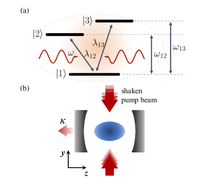
Figure 1: (a) Three-level system coupled to a single light mode. (b) Schematic diagram of the shaken atom-cavity system. The cavity photon loss rate is $\kappa$. This atom-cavity configuration can emulate the driven-dissipative three-level Dicke model.

II Three-level Dicke Model

We are interested in the properties of the three-level Dicke model for a system of $N$ three-level atoms interacting with a quantised light mode, as schematically shown in Fig. 1(a). Each atom has three energy states $|1\rangle$, $|2\rangle$, and $|3\rangle$. We define the three-level Dicke model by the Hamiltonian,

$$H/\hbar =\omega\hat{a}^{\dagger}\hat{a}+\omega_{\mathrm{12}}\hat{J}^{12}_{z}+\omega_{\mathrm{13}}\hat{J}^{\mathrm{13}}_{z}$$ (1)

$$+\frac{2}{\sqrt{N}}\left(\hat{a}^{\dagger}+\hat{a}\right)\left(\lambda_{12}\hat{J}^{\mathrm{12}}_{x}+\lambda_{13}\hat{J}^{\mathrm{13}}_{x}\right),$$

where $\omega$ is the photon frequency, $\omega_{nm}$ is the detuning between states $|m\rangle$ and $|n\rangle$, and $\lambda_{nm}$ is the light-matter interaction strength associated with the photon-mediated coupling between states $|n\rangle$ and $|m\rangle$. The bosonic operators $\hat{a}$ and $\hat{a}^{\dagger}$ annihilate and create a photon in the quantised light mode, respectively. There are three classes of pseudospin operators $\hat{J}^{12}_{\mu}$, $\hat{J}^{13}_{\mu}$, and $\hat{J}^{23}_{\nu}$ with $\mu\in\{z,\pm\}$ and $\nu\in\{\pm\}$, corresponding to the transitions $|1\rangle\leftrightarrow|2\rangle$, $|1\rangle\leftrightarrow|3\rangle$, and $|2\rangle\leftrightarrow|3\rangle$, respectively. These operators obey the commutation relation of the SU(3) algebra (see Appendix A). The $x$- and $y$-components of the pseudospins are defined as $\hat{J}^{\mathrm{\ell}}_{x}=(\hat{J}^{\mathrm{\ell}}_{+}+\hat{J}^{\mathrm{\ell}}_{-})/2$ and $\hat{J}^{\mathrm{\ell}}_{y}=(\hat{J}^{\mathrm{\ell}}_{+}-\hat{J}^{\mathrm{\ell}}_{-})/2i$, respectively with $\ell\in\{12,13,23\}$.

Note that, in principle, there is a light-matter coupling term proportional to $\hat{J}^{\mathrm{23}}_{x}$ in Eq. (1) Sung and Bowden (1979). However, this term is neglected here since we are only interested in the case when $\omega_{12}\approx\omega_{13}$. This leads to a negligibly small $\lambda_{23}$ since the light-matter coupling strength is proportional to the energy difference between the relevant states Sakurai and Napolitano (2017); Baksic et al. (2013). Moreover, we could also use the Gell-Mann matrices as the representation of the SU(3) group in our system. To retain a form of the Hamiltonian reminiscent of the standard two-level Dicke model, which is often written using a representation of the SU(2) group, we instead use the pseudospin operators as described above. Nevertheless, the Gell-Mann matrices can be obtained from appropriate superpositions of the pseudospin operators (see Appendix A).

The Hamiltonian in Eq. (1) is, superficially, similar to the two-component Dicke model Landini et al. (2018); Chiacchio and Nunnenkamp (2019); Buča and Jaksch (2019); Dogra et al. (2019) (see also Appendix B for a brief discussion). However, we emphasise that unlike in the two-component Dicke model, which describes two types of two-level systems coupled through the light field, the pseudospin operators introduced in Eq. (1) obey the SU(3) algebra resulting from the use of three-level systems. This fundamentally changes the dynamics of the parametrically driven system out of equilibrium since new terms corresponding to additional spin operators are now present in the equations of motion.

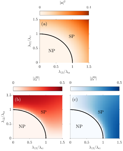
Figure 2: Long-time average of the mean-field dynamics of the (a) cavity mode occupation $|a|^{2}$, (b) $|j^{12}_{x}|^{2}$, and (c) $|j^{13}_{x}|^{2}$ for $\omega=\omega_{12}=\omega_{13}=\kappa$. The black curve denotes the critical line separating the normal and superradiant phases in the thermodynamic limit.

II.1 Holstein-Primakoff transformation

To obtain analytical predictions of the phase boundaries, we employ a Holstein-Primakoff (HP) approximation in the thermodynamic limit, i.e. $N\rightarrow\infty$. This leads to the following Hamiltonian

$$H/\hbar =\omega\hat{a}^{\dagger}\hat{a}+\omega_{12}\hat{a}^{\dagger}_{12}\hat{a}_{12}+\omega_{13}\hat{a}^{\dagger}_{13}\hat{a}_{13}$$ (2)

$$+\left(\hat{a}^{\dagger}+\hat{a}\right)\left[\lambda_{12}(\hat{a}^{\dagger}_{12}+\hat{a}_{12})+\lambda_{13}(\hat{a}^{\dagger}_{13}+\hat{a}_{13})\right]~{}.$$

We obtain an elliptic equation for the critical light-matter coupling from the stability matrix (see Appendix C for details)

$$\frac{\left(\kappa^{2}+\omega^{2}\right)}{4\omega}=\left(\frac{\lambda^{2}_{12}}{\omega_{12}}+\frac{\lambda^{2}_{13}}{\omega_{13}}\right).$$ (3)

In the standard open Dicke model, $\lambda_{13}=0$, the critical light-matter coupling, $\lambda_{\mathrm{cr}}=\sqrt{(\kappa^{2}+\omega^{2})\left(\omega_{12}/\omega\right)}/2$, is recovered Dimer et al. (2007). To illustrate the resulting phases, we consider the case $\omega=\omega_{12}=\omega_{13}$. Then, the critical line in Eq. (3) defines a circle in the parameter space spanned by $\lambda_{12}$ and $\lambda_{13}$, as seen in Fig. 2. For combinations of light-matter coupling strengths $\{\lambda_{12},\lambda_{13}\}$ within the area enclosed by Eq. (3), the stable phase corresponds to a normal phase (NP), while those outside the area will lead to an instability towards the formation of a superradiant phase (SP).

II.2 Phase diagram

Next, we employ a mean-field approximation $\langle\hat{a}\hat{J}^{\ell}_{\mu}\rangle\approx\langle\hat{a}\rangle\langle\hat{J}^{\ell}_{\mu}\rangle$ starting from Eq. (1) to obtain the dynamics of the system in a semiclassical approximation (see Appendix D for details). This approximation becomes exact in the thermodynamic limit $N\rightarrow\infty$ in or near the steady state. Furthermore, we introduce the rescaled $c$-numbers $a\equiv\langle\hat{a}\rangle/\sqrt{N}$ and $j^{\ell}_{\mu}\equiv\langle\hat{J}^{\ell}_{\mu}\rangle/N$. The resulting mean-field equations of motion that we simulate are shown in Appendix E. We further note that the SU(3) group inherits two Casimir charges, a quadratic $C_{1}$ and a cubic $C_{2}$. In contrast to this, the group SU(2) has only one quadratic Casimir charge, namely the total spin $J^{2}=(J_{x})^{2}+(J_{y})^{2}+(J_{z})^{2}$. The expressions for the charges are shown in Appendix A. We track these quantities when solving the equations of motion to ensure convergence of our numerical results. In our simulations, we initialise in the normal phase $j^{\ell}_{\mu}=0$, except for $j^{12}_{z}=j^{13}_{z}=-1/2$. This amounts to all the atoms initially occupying the lowest energy state $|1\rangle$. We initialise the cavity field as $a=10^{-2}$.

An observable of interest is the occupation of the photonic mode $|a|^{2}$ as this differentiates the normal $(|a|^{2}\rightarrow 0$ for $N\rightarrow\infty$ ) and superradiant ($|a|^{2}>0$) phases. Moreover, we are interested in the magnitude of the $x$-component of the collective spin operators corresponding to the transition $|1\rangle\leftrightarrow|2\rangle$ and $|1\rangle\leftrightarrow|3\rangle$, which are $|j^{12}_{x}|$ and $|j^{13}_{x}|$, respectively. In Fig. 2, we present the long-time average of $|a|^{2}$, $|j^{12}_{x}|$ and $|j^{13}_{x}|$, calculated from numerically solving the equations of motion. Similar to the standard two-level Dicke model Kirton et al. (2019), the photonic mode occupation or the $x$-component of the pseudospin operators can be regarded as order parameters, as they are zero in the NP and are nonzero in the SP. Furthermore, we demonstrate in Fig. 2 that the onset of superradiance according to our mean-field dynamics agrees with the analytical critical line defined by Eq. (3). In the superradiant phase, $|j^{12}_{x}|>|j^{13}_{x}|$ for $\lambda_{12}>\lambda_{13}$ and $|j^{12}_{x}|<|j^{13}_{x}|$ for $\lambda_{12}<\lambda_{13}$, as inferred from Figs. 2(b) and 2(c).

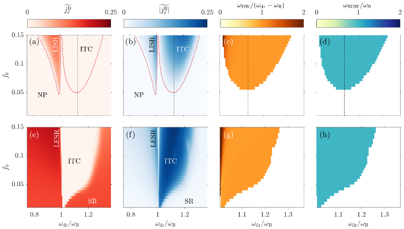
Figure 3: Dynamical phase diagram for (a)-(d) $\lambda=0.98\lambda_{\mathrm{cr}}$ and (e)-(f) $\lambda=1.02\lambda_{\mathrm{cr}}$. Time-averaged (a), (e) $\widetilde{j^{\mathrm{D}}_{x}}$ and (b), (f) $\widetilde{|j^{\mathrm{B}}_{x}|}$ taken over 100 driving cycles, $\tau=100T$, for varying modulation parameters. The dominant or peak frequency in the power spectrum of (c), (g) $j^{\mathrm{D}}_{x}$ and (d),(h) $j^{\mathrm{B}}_{x}$ for $\omega_{\mathrm{dr}}>\omega_{\mathrm{B}}$. The dotted lines in (a) and (b) denote the instability boundary according to the oscillator model. In (c), (d), (g), and (h), we are only showing the response frequencies $\omega_{\mathrm{DW}}$ and $\omega_{\mathrm{BDW}}$ for parameter sets, which yield $\widetilde{|j^{\mathrm{B}}_{x}|}>0.01$ and $\widetilde{j^{\mathrm{D}}_{x}}<0$. Note that we are rescaling the response frequencies in (c) and (g) to $\omega_{\mathrm{DW}}/(\omega_{\mathrm{dr}}-\omega_{\mathrm{B}})$ and it is rescaled in (d) and (h) to $\omega_{\mathrm{BDW}}/\omega_{\mathrm{B}}$. The vertical dashed line in (a)-(d) corresponds to the sum frequency $\omega_{\mathrm{sum}}=\omega_{\mathrm{LP}}+\omega_{\mathrm{B}}$.

III Parametrically Driven Open three-level Dicke model

We now explore the parametrically driven three-level Dicke model by the Hamiltonian

$$H/\hbar =\omega\hat{a}^{\dagger}\hat{a}+\omega_{\mathrm{D}}\hat{J}^{\mathrm{D}}_{z}+\omega_{\mathrm{B}}\hat{J}^{\mathrm{B}}_{z}+2\phi(t)(\omega_{\mathrm{B}}-\omega_{\mathrm{D}})\hat{J}^{\mathrm{DB}}_{x}$$ (4)

$$+\frac{2\lambda}{\sqrt{N}}\left(\hat{a}^{\dagger}+\hat{a}\right)\left(\hat{J}^{\mathrm{D}}_{x}-\phi(t)\hat{J}^{\mathrm{B}}_{x}\right).$$

This particular choice of the Hamiltonian is motivated by its connection to the shaken atom-cavity system, which we will demonstrate and explore in more detail later. Comparing with the undriven case in Eq. (1), it can be seen that $\omega_{12}=\omega_{\mathrm{D}}$, $\omega_{13}=\omega_{\mathrm{B}}$, $\hat{J}^{12}_{\mu}=\hat{J}^{\mathrm{D}}_{\mu}$, $\hat{J}^{13}_{\mu}=\hat{J}^{\mathrm{B}}_{\mu}$, $\lambda_{12}=\lambda$. We define $\phi(t)=f_{0}\sin(\omega_{\mathrm{dr}}t)$, which then means that $\lambda_{13}=-f_{0}\sin(\omega_{\mathrm{dr}}t)\lambda$. This labelling is motivated by the association of the pseudospins with the density wave states in the atom-cavity setup discussed later in Sec. IV. For now, we simply note that the photonic mode corresponds to a single cavity mode while the operators $\hat{J}^{\mathrm{D}}_{\mu}$ and $\hat{J}^{\mathrm{B}}_{\mu}$ are associated with the density wave (DW) and bond-density wave (BDW) states in the shaken atom-cavity system, respectively Cosme et al. (2019). A small term proportional to $\hat{J}^{\mathrm{23}}_{x}\equiv\hat{J}^{\mathrm{DB}}_{x}$ is included in Eq. (4) since this will appear later when we show how the atom-cavity system can be mapped onto the specific form of the parametrically driven three-level Dicke model Eq. (4).

III.1 Holstein-Primakoff transformation

In Sect. II.1, we have applied the HP transformation to the undriven system described by Eq. (2). We now extend this analysis to include the driving term. Applying the transformation and identifying $\hat{d}\equiv\hat{a}_{\mathrm{12}}$ and $\hat{b}\equiv\hat{a}_{\mathrm{13}}$, we obtain a HP Hamiltonian shown in Eq. (F20) of Appendix F. In particular, we are interested in $d\equiv\langle\hat{d}\rangle$ and $b\equiv\langle\hat{b}\rangle$.

We recall that for a quantum harmonic oscillator $\hat{f}^{\dagger}=\sqrt{\omega_{F}/\hbar}(x_{F}-(i/\omega_{F})p_{F})$ and $\hat{f}=\sqrt{\omega_{F}/\hbar}(x_{F}+(i/\omega_{F})p_{F})$. Then, we can express the corresponding HP Hamiltonian in momentum-position representation as

$$H =\frac{\omega^{2}}{2}\hat{x}^{2}+\frac{\hat{p}^{2}}{2}+\frac{\omega_{\mathrm{D}}^{2}}{2}\hat{x}^{2}_{\mathrm{D}}+\frac{\hat{p}_{\mathrm{D}}^{2}}{2}+\frac{\omega_{\mathrm{B}}^{2}}{2}\hat{x}^{2}_{\mathrm{B}}+\frac{\hat{p}_{\mathrm{B}}^{2}}{2}$$ (5)

$$+2\lambda\sqrt{\omega\omega_{\mathrm{D}}}\hat{x}\hat{x}_{\mathrm{D}}-2\phi(t)\lambda\sqrt{\omega\omega_{\mathrm{B}}}\hat{x}\hat{x}_{\mathrm{B}}$$

$$+\phi(t)(\omega_{\mathrm{B}}-\omega_{\mathrm{D}})\sqrt{\omega_{\mathrm{D}}\omega_{\mathrm{B}}}\left(\hat{x}_{\mathrm{D}}\hat{x}_{\mathrm{B}}+\frac{\hat{p}_{\mathrm{D}}\hat{p}_{\mathrm{B}}}{\omega_{\mathrm{D}}\omega_{\mathrm{B}}}\right).$$

This has the form a Hamiltonian for three coupled oscillators: (i) cavity oscillator, (ii) DW oscillator, and (iii) BDW oscillator with frequencies $\omega$, $\omega_{\mathrm{D}}$, and $\omega_{\mathrm{B}}$, respectively. Here, the two coupling constants connecting the BDW oscillator to the cavity and DW oscillators are periodically switched on and off or parametrically driven. Interestingly, due to the shaking of the pump, the momenta of the DW and BDW oscillators are also periodically coupled as seen from the last term in Eq. (5). However, we find that this does not alter the qualitative features of the dynamics, as shown in Fig. 8 in the Appendix E.

We initialise the system in the normal state corresponding to having $d=0$ and $b=0$, which amounts to the absence of bosons in the excited states $|2\rangle$ and $|3\rangle$, respectively. Note that a small non-zero occupation of the photonic mode $\langle\hat{a}\rangle\equiv a=10^{-2}$ is necessary to push the system out of the normal phase when it becomes an unstable state Chiacchio and Nunnenkamp (2019). The dynamics is obtained according to Eq. (F21) for varying driving strength $f_{0}$ and driving frequency $\omega_{\mathrm{dr}}$. A parametric resonance in a linear system corresponding to a bilinear Hamiltonian, such as the simplified toy model Eq. (F20), manifests itself as an oscillatory solution with exponentially diverging amplitude. The dotted curves in Figs. 3(a)-(d) denote the points in the $(\omega_{\mathrm{dr}},f_{0})$-space, where $(b+b^{*})$ exceeds unity within the first 100 driving cycles, signalling a diverging solution (see also Fig. 5). They indicate the regions where the normal phase is unstable towards a different collective phase.

We identify two resonances responsible for the driving-induced destabilisation of the normal phase: (i) resonance at the BDW oscillator frequency $\omega_{\mathrm{B}}$ and (ii) a sum resonance involving $\omega_{\mathrm{B}}$ and the lower polariton frequency $\omega_{\mathrm{LP}}$ of the atomic modes dressed by the cavity mode forming the lower polariton state Mivehvar et al. (2021). Note that we derive the expression for $\omega_{\mathrm{LP}}$ within the HP approach and we describe our method for obtaining the lower polariton frequency by exploiting a parametric resonance in Appendix G. The resonance frequencies are identified as the driving frequencies with the lowest modulation strength needed to induce an exponential instability. For $\omega_{\mathrm{dr}}<\omega_{\mathrm{B}}$, the resonance frequency is close to $\omega_{\mathrm{B}}$. For $\omega_{\mathrm{dr}}>\omega_{\mathrm{B}}$, the sum resonance at $\omega_{\mathrm{sum}}=\omega_{\mathrm{B}}+\omega_{\mathrm{LP}}$ is the main mechanism, as highlighted by the vertical dashed line in Figs. 3(a)-(d) (see also Fig. 5).

III.2 Dynamical phase diagrams

To further understand the resonant collective phases, we obtain the dynamics of the system. Within the mean-field approximation, we simulate the semiclassical equations of motion shown in Appendix E. Similar to the HP theory in the previous subsection, we initialise the system in the normal phase with small non-zero occupation of the photonic mode $a=10^{-2}$, We further choose $j^{\ell}_{\mu}=0$, except for $j^{\mathrm{D}}_{z}=j^{\mathrm{B}}_{z}=-1/2$. In addition to the photonic mode occupation $|a|^{2}$, we are also interested in the $x$-component of the pseudospins $j^{\mathrm{D}}_{x}$ and $j^{\mathrm{B}}_{x}$. Time is in units of the modulation period $T=2\pi/\omega_{\mathrm{dr}}$. The parameters for the simulation are shown in Appendix H.

In Fig. 4, we present exemplary dynamics for resonant modulation specifcially for $\omega_{\mathrm{dr}}=1.05\,\omega_{\mathrm{B}}$. We choose the light-matter coupling strengths close to the phase boundary between the normal and superradiant phases, specifically $\lambda=0.98\,\lambda_{\mathrm{cr}}$ and $\lambda=1.02\,\lambda_{\mathrm{cr}}$, respectively. In the absence of driving, $f_{0}=0$, we reproduce the prediction of a normal phase NP and superradiant phase SP from the standard two-level Dicke model. Periodic driving closed to but blue-detuned from $\omega_{\mathrm{B}}$ leads to similar long-time behaviour for $\lambda<\lambda_{\mathrm{cr}}$ and $\lambda>\lambda_{\mathrm{cr}}$. That is, the spin components related to the order parameters in the atom-cavity system, $j^{\mathrm{D}}_{x}$ and $j^{\mathrm{B}}_{x}$, periodically changes their sign concomitant to pulses of light being emitted. The slow subharmonic oscillations in $j^{\mathrm{D}}_{x}$, as exemplified in Fig. 4(b), reflects the temporal periodicity of the entire light-matter system. Note that, $j^{\mathrm{B}}_{x}$ rapidly switches sign, as shown in Figs. 4(c) and 4(f).

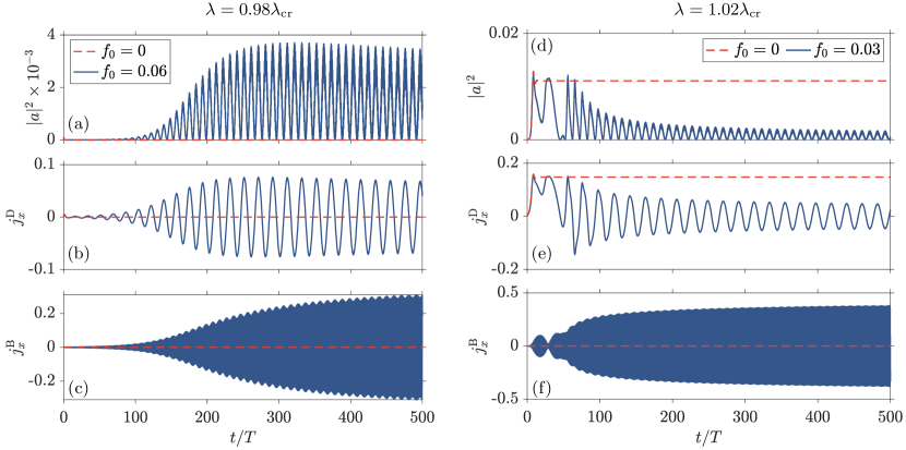
Figure 4: Comparison between unmodulated and resonantly modulated dynamics for light-matter coupling strengths close to the NP-SR phase of the unmodulated system, (a)-(c) $\lambda=0.98\lambda_{\mathrm{cr}}$ and (d)-(f) $\lambda=1.02\lambda_{\mathrm{cr}}$. The relevant observables are the (a),(d) cavity mode occupation $|a|^{2}$, and the order parameters (b),(e) $j^{\mathrm{D}}_{x}$ and (c),(f) $j^{\mathrm{B}}_{x}$. The modulation frequency is fixed at $\omega_{\mathrm{dr}}=1.05\omega_{\mathrm{B}}$.

We quantify the dynamical regimes in the system using the response frequencies $\omega_{\mathrm{DW}}$ and $\omega_{\mathrm{BDW}}$, which we define as the frequency at which $j^{\mathrm{D}}_{x}$ and $j^{\mathrm{B}}_{x}$ has a maximum in the power spectrum. Considering blue-detuned driving with respect to the BDW oscillator frequency $\omega_{\mathrm{dr}}>\omega_{\mathrm{B}}$, we find that the DBDW phase is characterised by fast oscillations of $j^{\mathrm{B}}_{x}$ at $\omega_{\mathrm{BDW}}=\omega_{\mathrm{B}}$ and slow oscillations of $j^{\mathrm{D}}_{x}$ at $\omega_{\mathrm{DW}}=\omega_{\mathrm{dr}}-\omega_{\mathrm{B}}$. These observations are valid for both $\lambda<\lambda_{\mathrm{cr}}$ and $\lambda>\lambda_{\mathrm{cr}}$, as demonstrated in Figs. 3(c), 3(d), 3(g), and 3(h), where the relations $\omega_{\mathrm{DW}}/(\omega_{\mathrm{dr}}-\omega_{\mathrm{B}})=1$ and $\omega_{\mathrm{BDW}}/\omega_{\mathrm{B}}=1$ are satisfied over a wide range modulation parameters. In general, the system’s response frequency $\omega_{\mathrm{DW}}$ is subharmonic and incommensurate with respect to the driving frequency $\omega_{\mathrm{dr}}$, underpinning the classification of the DBDW phase as an ITC. Thus, we show that the emergence of the ITC phase is one of the signatures of the parametrically driven three-level Dicke model. In contrast, the system has a harmonic response, meaning that $|a|^{2}$ and $j^{\mathrm{D}}_{x}$ have the same response frequency $\omega_{\mathrm{DW}}=2\omega_{\mathrm{dr}}$ Cosme et al. (2019), for combinations of driving parameters outside the dark areas in Figs. 3(c), 3(d), 3(g), and 3(h), including red-detuned driving $\omega_{\mathrm{dr}}<\omega_{\mathrm{B}}$.

In the ITC phase for $\omega_{\mathrm{dr}}>\omega_{\mathrm{B}}$, the oscillations of $j^{\mathrm{D}}_{x}$ and $j^{\mathrm{B}}_{x}$ around zero translate to vanishing time-averaged values,

$$\widetilde{j^{\mathrm{\ell}}_{x}}=\frac{1}{\tau}\int_{0}^{\tau}j^{\mathrm{\ell}}_{x}\,dt.$$ (6)

This property is visible in the light area in Fig. 3(e). Note, however, that even though $\widetilde{j^{\mathrm{D}}_{x}}=0$, the time-averaged cavity mode occupation $\widetilde{|a|^{2}}$ does not necessarily vanish, especially when ${j^{\mathrm{D}}_{x}}$ has nonzero oscillation amplitude, as shown in Figs. 3(a) and 5(a). The normal phase has ${j^{\mathrm{D}}_{x}}=0$ for all times and as such, $\widetilde{|j^{\mathrm{D}}_{x}|}$ also vanishes, albeit trivially, similar to the ITC phase. Therefore, to distinguish between the normal phase and the ITC phase, we calculate $\widetilde{|j^{\mathrm{B}}_{x}|}$, a quantity that vanishes for the normal phase and is nonzero for the ITC phase. In Figs. 3(b) and 3(f), it can be seen that the BDW states are resonantly excited not only for the ITC phase in $\omega_{\mathrm{dr}}>\omega_{\mathrm{B}}$ but also for red-detuned driving $\omega_{\mathrm{dr}}<\omega_{\mathrm{B}}$. We emphasise that the dynamical response for $\omega_{\mathrm{dr}}<\omega_{\mathrm{B}}$ remains harmonic, making this phase distinct from the ITC, normal, and superradiant phases.

We now focus on red-detuned driving $\omega_{\mathrm{dr}}<\omega_{\mathrm{B}}$ to illustrate the effects of resonantly exciting the BDW states in this case. For $\lambda<\lambda_{\mathrm{cr}}$, the normal phase, expected to be dominant in the absence of driving, is suppressed, which then gives rise to a superradiant phase enabled by the excitation of the BDW states. We call this resonant phase for $\lambda<\lambda_{\mathrm{cr}}$ and $\omega_{\mathrm{dr}}<\omega_{\mathrm{B}}$ the light-induced superradiant (LISR) phase. In this phase, the long-time average of the cavity mode occupation $|a|^{2}$ and $j^{\mathrm{D}}_{x}$ are both nonzero, similar to the superradiant phase, as seen from the resonance lobe in Figs. 3(a) and 5(a) for $\omega_{\mathrm{dr}}<\omega_{\mathrm{B}}$. However, the occupation of BDW states, demonstrated in Fig. 3(b), distinguishes the LISR phase from the usual SR phase in the undriven case. An analogous effect for $\lambda>\lambda_{\mathrm{cr}}$ is the enhancement of the superradiant phase, the stationary phase in the absence of driving. This light-enhanced superradiant (LESR) phase is identified by an increase in $|a|^{2}$ and $j^{\mathrm{D}}_{x}$, accompanied by large amplitude oscillations of $j^{\mathrm{B}}_{x}$, as shown in Figs. 5(b), 3(e), and 3(f). In addition to the ITC phase, the presence of LISR and LESR phases, depending on $\lambda$, is another signature of the driven-dissipative three-level Dicke model.

IV Emulation using a Shaken Atom-Cavity system

We now show that the parametrically driven open three-level Dicke model can be emulated by a shaken atom-cavity system. To this end, we first describe the many-body Hamiltonian of the shaken atom-cavity. Then, we present the approximation needed to obtain Eq. (4) from the atom-cavity Hamitlonian.

IV.1 Shaken atom-cavity Hamiltonian

We consider a minimal model for describing the dynamics along the pump and cavity directions of an atom-cavity system schematically depicted in Fig. 1(b). The corresponding many-body Hamiltonian is given by Cosme et al. (2019)

$$\hat{H} /\hbar=-\delta_{\mathrm{C}}\hat{a}^{\dagger}\hat{a}+\int dydz\hat{\Psi}^{\dagger}(y,z)\biggl{[}-\frac{\hbar}{2m}\nabla^{2}$$ (7)

$$-\omega_{\mathrm{rec}}\epsilon_{\mathrm{p}}\cos^{2}(ky+\phi(t))+U_{0}\hat{a}^{\dagger}\hat{a}\cos^{2}(kz)$$

$$-\sqrt{\omega_{\mathrm{rec}}|U_{0}|\epsilon_{\mathrm{p}}}\cos(ky+\phi(t))\cos(kz)(a^{\dagger}+a)\biggr{]}\hat{\Psi}(y,z),$$

where $\hat{a}$ ($\hat{a}^{\dagger}$) annihilates (creates) a photon in the single-mode cavity and $\hat{\Psi}(y,z)$ is the bosonic field operator for the atoms with mass $m$. The pump-cavity detuning is $\delta_{\mathrm{C}}$. The frequency shift per atom is taken to be red-shifted $U_{0}<0$. The pump intensity $\epsilon_{\mathrm{p}}$ is measured in units of the recoil energy $E_{\mathrm{rec}}=\hbar^{2}k^{2}/2m$, where the wavevector is $k=2\pi/\lambda_{\mathrm{p}}$. Note that in Eq. (7), we neglect the effects of short-range collisional interaction. The pump lattice is periodically shaken by introducing a time-dependent phase in the pump mode

$$\phi(t)=f_{0}\sin(\omega_{\mathrm{dr}}t),$$ (8)

where $f_{0}$ is the unitless modulation strength and $\omega_{\mathrm{dr}}$ is the modulation frequency. The characteristic timescale is thus set by the driving period $T=2\pi/\omega_{\mathrm{dr}}$.

The dynamics of the atom-cavity system follows from the Heisenberg-Langevin equations Ritsch et al. (2013); Mivehvar et al. (2021),

$$\frac{\partial}{\partial t}\hat{\Psi} =\frac{i}{\hbar}[\hat{H},\hat{\Psi}]$$ (9)

$$\frac{\partial}{\partial t}\hat{a} =\frac{i}{\hbar}[\hat{H},\hat{a}]-\kappa\hat{a}+\xi$$ (10)

where $\kappa$ is the cavity dissipation rate and the associated fluctuations are captured by the noise term $\xi$ satisfying $\langle\xi^{*}(t)\xi(t^{\prime})\rangle=\kappa\delta(t-t^{\prime})$. In the mean-field limit of large particle number $N$, quantum fluctuations are neglected and the bosonic operators can be approximated as $c$-numbers. The dynamics can then be obtained by numerically solving the resulting coupled differential equations corresponding to the equations of motion of the system. This approach and its extension beyond a mean-field approximation have been successfully used to predict and observe various dynamical phases in the transversely pumped atom-cavity system from a driving-induced renormalisation of the phase boundary to time crystals Cosme et al. (2018); Georges et al. (2018); Cosme et al. (2019); Keßler et al. (2019, 2020, 2021); Georges et al. (2021).

IV.2 Low-momenta approximation

The atom-cavity system can be mapped onto the Dicke model using a low-momenta approximation. To this end, we assume that the majority of the atoms only occupy the five-lowest momentum modes, namely the zero-momentum mode, $|k_{y},k_{z}\rangle=|0,0\rangle$, and the states associated with the self-organised chequerboard phase, $|\pm k,\pm k\rangle$. These momentum modes are coupled by the scattering of photons between the pump and cavity fields. This low-momenta approximation is valid close to the phase boundary between the homogeneous BEC phase and the self-organised DW phase.

Resonant shaking has been shown to lead to the emergence of an incommensurate time crystal, where atoms localise at positions between the antinodes of the pump lattice Cosme et al. (2019); joi . That is, in addition to the spatial mode $\cos(ky)\cos(kz)$ in the DW phase, the atoms are driven into additional states, namely the BDW states, as the atomic distribution acquires an overlap with the spatial mode $\sin(ky)\cos(kz)$. Note that this mode is made available by the periodic shaking of the pump lattice since it explicitly breaks the spatial symmetry along the pump axis. Owing to how the system periodically switches between superpositions of DW and BDW states, we call this dynamical phase as the dynamical BDW (DBDW) phase. Since the DBDW phase has been previously identified as an incommensurate time crystal (ITC), we will use the term DBDW and ITC phase interchangeably.

The atomic field operator is expanded to include the relevant spatial modes

$$\hat{\Psi}(y,z)=\hat{c}_{1}+2~{}\hat{c}_{2}\cos(ky)\cos(kz)+2~{}\hat{c}_{3}\sin(ky)\cos(kz),$$ (11)

where the $c_{i}$ are bosonic annihilation and creation operator. We use this expansion in the many-body Hamiltonian Eq. (7). Evaluating the integrals within one unit cell and for weak driving $f_{0}\ll 1$, we obtain a Hamiltonian in a reduced subspace

$$H/\hbar=-\delta_{\mathrm{C}}\hat{a}^{\dagger}\hat{a}+2\omega_{\mathrm{rec}}(\hat{c}^{\dagger}_{2}\hat{c}_{2}+\hat{c}^{\dagger}_{3}\hat{c}_{3})+\frac{U_{0}}{2}\hat{a}^{\dagger}\hat{a}\biggl{[}\hat{c}^{\dagger}_{1}\hat{c}_{1}$$ (12)

$$+\frac{3}{2}(\hat{c}^{\dagger}_{2}\hat{c}_{2}+\hat{c}^{\dagger}_{3}\hat{c}_{3})\biggr{]}-\frac{\omega_{\mathrm{rec}}\epsilon_{\mathrm{p}}}{4}\biggl{[}2(\hat{c}^{\dagger}_{1}\hat{c}_{1}+\hat{c}^{\dagger}_{2}\hat{c}_{2}+\hat{c}^{\dagger}_{3}\hat{c}_{3})$$

$$+(\hat{c}^{\dagger}_{2}\hat{c}_{2}-\hat{c}^{\dagger}_{3}\hat{c}_{3})-2\phi(t)(\hat{c}^{\dagger}_{2}\hat{c}_{3}+\hat{c}^{\dagger}_{3}\hat{c}_{2})\biggr{]}-\frac{\sqrt{\omega_{\mathrm{rec}}|U_{0}|\epsilon_{\mathrm{p}}}}{2}$$

$$\qquad\times(\hat{a}^{\dagger}+\hat{a})\biggl{[}(\hat{c}^{\dagger}_{1}\hat{c}_{2}+\hat{c}^{\dagger}_{2}\hat{c}_{1})-\phi(t)(\hat{c}^{\dagger}_{1}\hat{c}_{3}+\hat{c}^{\dagger}_{3}\hat{c}_{1})\biggr{]}.$$

IV.3 Schwinger boson representation

We transform the bosonic operators in Eq. (12) into collective pseudospin operators through the Schwinger boson representation. The additional spatial mode $\sin(ky)\cos(kz)$ is described by the operator ${c}_{3}$, so the atomic motion is represented as a three-level system. We introduce the pseudospin operators obeying SU(3) algebra via

$$N =\hat{c}^{\dagger}_{1}\hat{c}_{1}+\hat{c}^{\dagger}_{2}\hat{c}_{2}+\hat{c}^{\dagger}_{3}\hat{c}_{3}$$ (13)

$$\hat{J}^{\mathrm{D}}_{+} =\hat{c}^{\dagger}_{2}\hat{c}_{1},\quad\hat{J}^{\mathrm{D}}_{-}=\hat{c}^{\dagger}_{1}\hat{c}_{2},\quad\hat{J}^{\mathrm{D}}_{z}=\frac{1}{2}\left(\hat{c}^{\dagger}_{2}\hat{c}_{2}-\hat{c}^{\dagger}_{3}\hat{c}_{3}-\hat{c}^{\dagger}_{1}\hat{c}_{1}\right),$$

$$\hat{J}^{\mathrm{B}}_{+} =\hat{c}^{\dagger}_{3}\hat{c}_{1},\quad\hat{J}^{\mathrm{B}}_{-}=\hat{c}^{\dagger}_{1}\hat{c}_{3},\quad\hat{J}^{\mathrm{B}}_{z}=\frac{1}{2}\left(\hat{c}^{\dagger}_{3}\hat{c}_{3}-\hat{c}^{\dagger}_{2}\hat{c}_{2}-\hat{c}^{\dagger}_{1}\hat{c}_{1}\right),$$

$$\hat{J}^{\mathrm{DB}}_{+} =\hat{c}^{\dagger}_{2}\hat{c}_{3},\quad\hat{J}^{\mathrm{DB}}_{-}=\hat{c}^{\dagger}_{3}\hat{c}_{2}.$$

This representation suggests that the operators $\hat{J}^{\mathrm{D}}_{\mu}$ are associated with the DW state while $\hat{J}^{\mathrm{B}}_{\mu}$ are related to the BDW state. Applying the commutation relations for the bosonic operators $[\hat{c}_{m},\hat{c}^{\dagger}_{n}]=\delta_{mn}$, we recover the same commutation relations for the pseudospin operators presented in Eq. (A). That is, we identify $\hat{J}^{\mathrm{D}}_{\mu}\equiv\hat{J}^{\mathrm{12}}_{\mu}$, $\hat{J}^{\mathrm{B}}_{\mu}\equiv\hat{J}^{\mathrm{13}}_{\mu}$, and $\hat{J}^{\mathrm{DB}}_{\mu}\equiv\hat{J}^{\mathrm{23}}_{\mu}$.

Substituting the Schwinger boson representation in Eq. (13) into Eq. (12) yields the driven-dissipative three-level Dicke model Eq. (4). Within the shaken-atom cavity platform, the effective cavity field frequency is $\omega=(3U_{0}N)/4-\delta_{\mathrm{C}}=U_{0}N/4-\delta_{\mathrm{eff}}$, the effective pump-cavity detuning is $\delta_{\mathrm{eff}}$, and the light-matter coupling strength is $\lambda/\sqrt{N}=-\sqrt{\omega_{\mathrm{rec}}\epsilon_{\mathrm{p}}|U_{0}|}/{2}$. The pump intensity $\epsilon_{\mathrm{p}}$ shifts the frequencies of the pair of two-level transitions, $\omega_{\mathrm{D}}=2\omega_{\mathrm{rec}}(1-\epsilon_{\mathrm{p}}/8)$ and $\omega_{\mathrm{B}}=2\omega_{\mathrm{rec}}(1+\epsilon_{\mathrm{p}}/8)$. We can infer from Eq. (4) that weak periodic shaking effectively leads to a parametric driving of the light-matter coupling between the cavity and the spin associated to the BDW state. With these correspondences, we find that indeed the shaken atom-cavity system can be approximated by the driven three-level Dicke model presented in Eq. (4) and discussed in Sect. III. Moreover, we can identify the order parameters of the self-organised density wave states, namely the DW order parameter $\Theta_{\mathrm{DW}}=\langle\cos(ky)\cos(kz)\rangle=j^{\mathrm{D}}_{x}$ and the BDW order parameter $\Theta_{\mathrm{BDW}}=\langle\sin(ky)\cos(kz)\rangle=j^{\mathrm{B}}_{x}$.

IV.4 Comparison with the full atom-cavity model

We compare the dynamics of the cavity mode occupation and the DW order parameter for the full atom-cavity model Eq. (7) and the effective three-level model according to Eq. (E17). The parameters for the simulation are shown in Appendix H. For results based on the full atom-cavity model Eq. (7), we numerically determine $\epsilon_{\mathrm{cr}}$ from the onset of intracavity photon number Cosme et al. (2019). Moreover, the BDW oscillator frequency $\omega_{\mathrm{B}}$ for the full atom-cavity model is extracted from the oscillation frequency of the BDW order parameter $\Theta_{\mathrm{BDW}}$ Cosme et al. (2019). We show in Fig. 5 the time-averaged occupation of the cavity mode $|a|^{2}$,

$$\widetilde{|a|^{2}}=\frac{1}{\tau}\int_{0}^{\tau}|a|^{2}\,dt,$$ (14)

for $\tau=100T$, as a function of modulation strength $f_{0}$ and modulation frequency $\omega_{\mathrm{dr}}$.

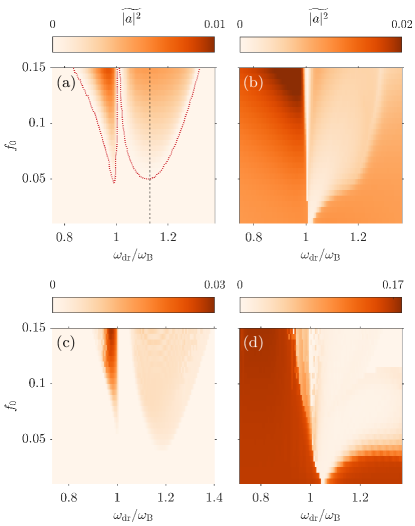
Figure 5: Time-averaged cavity mode occupation $|a|^{2}$ taken over 100 driving cycles, $\tau=100T$, according to (a),(b) the three-level Dicke model and (c),(d) the full atom-cavity model. For the three-level model, the light-matter coupling strengths are (a) $\lambda=0.98\lambda_{\mathrm{cr}}$ and (b) $\lambda=1.02\lambda_{\mathrm{cr}}$. The broken lines denote the instability boundary from the oscillator model. The vertical dashed line in (a) corresponds to the sum frequency $\omega_{\mathrm{sum}}=\omega_{\mathrm{LP}}+\omega_{\mathrm{B}}$ involving the lower polariton frequency $\omega_{\mathrm{LP}}$. $\omega_{\mathrm{LP}}$ has the value $\omega_{\mathrm{LP}}/2\pi\approx 1.06~{}\mathrm{kHz}$ for this example. For the full atom-cavity model, the pump strengths are (c) $\epsilon_{\mathrm{p}}=0.96\epsilon_{\mathrm{cr}}$ and (d) $\epsilon_{\mathrm{p}}=1.04\epsilon_{\mathrm{cr}}$, which corresponds to the $\lambda=0.98\lambda_{\mathrm{cr}}$ and $\lambda=1.02\lambda_{\mathrm{cr}}$, respectively.

For $\lambda<\lambda_{\mathrm{cr}}$, we obtain a qualitatively similar dynamical phase diagrams for the three-level Dicke model and the full atom-cavity model, as depicted in Figs. 5(a) and 5(c). Therefore, in this regime, the approximation of Eq. (7) via Eq. (4) is applicable. That is, the parametrically driven open three-level Dicke Hamiltonian is realized approximately by the shaken atom-cavity system. Moreover, the instability region from the oscillator model in the thermodynamic limit Eq. (F20) matches the onset of the cavity mode occupation in Fig. 5(a).

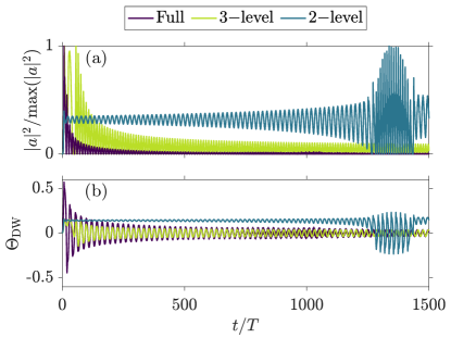
Figure 6: Comparison of the dynamics between the full atom-cavity model (in purple (black)), three-level (in green (light gray)), and coupled two-level Dicke model (in blue (dark gray)) for the (a) cavity mode occupation and (b) DW order parameter. For the Dicke models, the light-matter coupling strength is $\lambda=1.02\lambda_{\mathrm{cr}}$. This corresponds to a pump strength of $\epsilon_{\mathrm{p}}/\epsilon_{\mathrm{cr}}=1.04$ in the full-atom cavity model. The driving parameters are fixed to $f_{0}=0.03$ and $\omega_{\mathrm{dr}}=1.05\omega_{\mathrm{B}}$.

For $\lambda>\lambda_{\mathrm{cr}}$, the dark areas in Figs. 5(b) and 5(d) signify that the system has entered the DW or SR phase indicated by a nonvanishing cavity mode occupation, as expected for weak and off-resonant driving. However, the DW phase is suppressed for driving frequencies blue-detuned from $\omega_{\mathrm{B}}$ as indicated by the relative decrease in the cavity photon number in the light areas in Figs. 5(b) and 5(d). Crucially, the correspondence between Eqs. (7) and (4) breaks down for driving frequencies far-detuned from $\omega_{\mathrm{B}}$ as inferred from the parameter region $\omega_{\mathrm{dr}}>\omega_{\mathrm{B}}$ in Figs. 5(b) and 5(d). This can be attributed to the occupation of higher momentum modes, specifically $|\pm 2k,0\rangle$, in the full atom-cavity system Cosme et al. (2019), which is not captured in the low-momentum expansion Eq. (11) utilised in the mapping. Nevertheless, we still find good agreement on the qualitative features for driving frequencies near $\omega_{\mathrm{B}}$.

We also consider the dynamics according to a coupled two-level Dicke model for the same set of parameters (see Appendix B for details). In Fig. 6, we present the dynamics for $\lambda>\lambda_{\mathrm{cr}}$ with a driving frequency blue-detuned with respect to $\omega_{\mathrm{B}}$. The results of the coupled two-level systems clearly do not capture the dynamics of the full atom-cavity system. On the other hand, the three-level Dicke model and the full atom-cavity model predict the same dynamical response, which is a subharmonic motion exhibited as a pulsating photon number (see Fig. 6(a)) and a periodic switching of the sign of the DW order parameter (see Fig. 6(b)). This further supports our claim that the mapping between the three-level Dicke model and the full-atom cavity system is applicable to $\lambda>\lambda_{\mathrm{cr}}$ for as long as the driving frequency is close to $\omega_{\mathrm{B}}$. Note, however, that the coupled two-level systems model and the three-level model agree with each other for off-resonant driving when $j^{\mathrm{B}}_{x}\approx 0$, as demonstrated in Appendix B.

V Conclusions

In this work, we have investigated a three-level Dicke model, and derived its equilibrium phase diagram, which features a normal phase and a superradiant phase. We advanced the model to a driven-dissipative system, by including a dissipation mechanism via photon loss and a periodic driving process. For this system,we developed the dynamical phase diagram, which shows the phases for varying driving parameters, utilizing analytical and numerical methods. As a central result we have characterized the regime of an incommensurate time crystalline state in the phase diagram. Furthermore, we obtained light-enhanced and light-induced superradiant states, in which the equilibrium superradiant state is dynamically stabilized. As a physical system that can be naturally approximated via the three-level Dicke model, we have identified a periodically shaken atom-cavity system. While the non-shaken atom-cavity system can be approximated via the standard two-level Dicke model, the shaking induces the atoms to populate additional states that are modeled via a third state in the three-level Dicke model. We note that the LISR and LESR phases display similarities with light-induced Fausti et al. (2011) and light-enhanced superconductivity Hu et al. (2014), for which mechanisms have been proposed that involve the excitation of auxiliary modes, such as phonons Mankowsky et al. (2014); Denny et al. (2015); Okamoto et al. (2016) and Higgs bosons Homann et al. (2021), by means of optical pumping. Photoexcitation of the Higgs mode in cuprate superconductors has also been predicted to lead to an incommensurate time crystal Homann et al. (2020). In this work, the BDW state plays the role of such an auxiliary mode, as its excitation (or equivalently, the $|1\rangle\rightarrow|3\rangle$ in Fig. 1(a)) can be used to dynamically control the system to induce or enhance superradiance, or to enter a genuine dynamical order, namely the incommensurate time crystalline phase. We therefore expand the dynamical control of phases in atom-cavity systems to include light-induced and light-enhanced superradiance, in addition to the previously observed light-enhanced BEC or normal phase Cosme et al. (2018); Georges et al. (2018).

Note: During submission of this work, a subsequent example of the driven three-level Dicke model was presented in Lin et al. (2021).

Appendix A The SU(3) algebra, Gell-Mann matrices and the Casimir charges

$$[\hat{J}^{12}_{z},\hat{J}^{12}_{\pm}] =\pm\hat{J}^{12}_{\pm},\quad[\hat{J}^{12}_{-},\hat{J}^{12}_{+}]=2\hat{J}^{12}_{z}+\hat{J}^{13}_{z}+\frac{N}{2},$$

$$[\hat{J}^{13}_{z},\hat{J}^{13}_{\pm}] =\pm\hat{J}^{13}_{\pm},\quad[\hat{J}^{13}_{-},\hat{J}^{13}_{+}]=2\hat{J}^{13}_{z}+\hat{J}^{12}_{z}+\frac{N}{2},$$

$$[\hat{J}^{12}_{\pm},\hat{J}^{13}_{\mp}] =\pm\hat{J}^{23}_{\pm},\quad[\hat{J}^{23}_{+},\hat{J}^{23}_{-}]=\hat{J}^{12}_{z}-\hat{J}^{13}_{z},$$

$$[\hat{J}^{12}_{z},\hat{J}^{23}_{\pm}] =\pm\hat{J}^{23}_{\pm},\quad[\hat{J}^{13}_{z},\hat{J}^{23}_{\pm}]=\mp\hat{J}^{23}_{\pm},$$

$$[\hat{J}^{12}_{\pm},\hat{J}^{23}_{\mp}] =\mp\hat{J}^{13}_{\pm},\qquad[\hat{J}^{13}_{\pm},\hat{J}^{23}_{\pm}]=\mp\hat{J}^{12}_{\pm}.$$ (A1)

The remaining commutators not listed above vanish. Our choice of pseudospin operators for the SU(3) algebra can be mapped onto the Gell-Mann matrices Georgi (2018) via

$$F_{1}\equiv J^{12}_{x}=\frac{1}{2}\lambda_{1},$$

$$F_{2}\equiv J^{12}_{y}=\frac{1}{2}\lambda_{2},$$

$$F_{3}\equiv J^{12}_{z}+\frac{1}{2}J^{13}_{z}+N/4=\frac{1}{2}\lambda_{3},$$

$$F_{4}\equiv J^{23}_{x}=\frac{1}{2}\lambda_{4},$$

$$F_{5}\equiv J^{23}_{y}=\frac{1}{2}\lambda_{5},$$

$$F_{6}\equiv J^{13}_{x}=\frac{1}{2}\lambda_{6},$$

$$F_{7}\equiv-J^{13}_{y}=\frac{1}{2}\lambda_{7},$$

$$F_{8}\equiv-\frac{\sqrt{3}}{2}(J^{13}_{z}+N/6)=\frac{1}{2}\lambda_{8}.$$ (A2)

A.1 Casimir charges

The group SU(3) enjoys two Casimirs, which can be written in matrix form using the Gell-Mann basis as

$$C_{1} =\sum^{8}_{i=1}F_{i}F_{i}$$ (A3)

$$C_{2} =\sum^{8}_{j,k,l=1}d_{jkl}F_{j}F_{k}F_{l}$$ (A4)

with

$$d_{jkl}=\frac{1}{4}\mathrm{Tr}\left(\{\lambda_{j},\lambda_{k}\}\lambda_{l}\right).$$ (A5)

In our chosen basis, they take the form of

$$\langle C_{1}\rangle/N =\frac{1}{12}+\left(j^{12}_{x}\right)^{2}+\left(j^{12}_{y}\right)^{2}+\left(j^{12}_{z}\right)^{2}+\left(j^{13}_{x}\right)^{2}+\left(j^{13}_{y}\right)^{2}+\left(j^{13}_{z}\right)^{2}+\left(j^{23}_{x}\right)^{2}+\left(j^{23}_{y}\right)^{2}+\frac{1}{2}\left(j^{12}_{z}+j^{13}_{z}+2j^{12}_{z}j^{13}_{z}\right)$$ (A6)

$$\langle C_{2}\rangle/N^{3/2} =\frac{1}{72}\left\{-18\left(j^{12}_{y}\right)^{2}+216j^{23}_{y}(j^{12}_{y}j^{13}_{x}-j^{12}_{x}j^{13}_{y})+216j^{23}_{x}(j^{12}_{x}j^{13}_{x}+j^{12}_{y}j^{13}_{y})\right.$$

$$\left.-(1+6j^{12}_{z})\left[1+3j^{12}_{z}+18\left(j^{13}_{x}\right)^{2}+18\left(j^{13}_{y}\right)^{2}\right]-9j^{13}_{z}+36\left(j^{23}_{x}\right)^{2}(1+3j^{12}_{z}+3j^{13}_{z})\right.$$

$$\left.+36\left(j^{23}_{y}\right)^{2}(1+3j^{12}_{z}+3j^{13}_{z})-18\left[\left(j^{12}_{x}\right)^{2}(1+6j^{13}_{z})+j^{13}_{z}\left(6\left(j^{12}_{y}\right)^{2}+j^{13}_{z}+2j^{12}_{z}(2+3j^{12}_{z}+3j^{13}_{z})\right)\right]\right\}~{}.$$

Appendix B Two-Component Dicke Model

A modified version of the two-component Dicke model Chiacchio and Nunnenkamp (2019); Buča and Jaksch (2019), which can be realised in a spinor BEC coupled to an optical cavity Landini et al. (2018); Dogra et al. (2019), is given by

$$H/\hbar =\omega\hat{a}^{\dagger}\hat{a}+\omega_{\mathrm{1}}\hat{J}^{1}_{z}+\omega_{\mathrm{2}}\hat{J}^{\mathrm{2}}_{z}$$ (B7)

$$+\frac{2}{\sqrt{N}}\left(\hat{a}^{\dagger}+\hat{a}\right)\left(\lambda_{1}\hat{J}^{\mathrm{1}}_{x}+\lambda_{2}\hat{J}^{\mathrm{2}}_{x}\right).$$

Note that this has the same form as the three-level Hamiltonian in Eq. (1) except that here, the pseudospin operators fulfil to the SU(2) group algebra with the commutation relations,

$$[\hat{J}^{\ell}_{z},\hat{J}^{\ell}_{\pm}]=\pm\hat{J}^{\ell}_{\pm},\quad[\hat{J}^{\ell}_{-},\hat{J}^{\ell}_{+}]=2\hat{J}^{\ell}_{z},$$ (B8)

where $\ell\in\{1,2\}$. Applying the same mean-field approximation as in Sec. II.2, we obtain the following equations of motion consistent with those in Refs. Landini et al. (2018); Chiacchio and Nunnenkamp (2019); Buča and Jaksch (2019); Dogra et al. (2019),

$$\frac{da}{dt} =-(i\omega+\kappa)a-i2\sum^{2}_{\ell=1}\lambda_{\ell}j^{\ell}_{x}$$ (B9)

$$\frac{dj^{\ell}_{x}}{dt} =-\omega_{\mathrm{\ell}}j^{\ell}_{y}$$

$$\frac{dj^{\ell}_{y}}{dt} =\omega_{\mathrm{\ell}}j^{\ell}_{x}-2\lambda_{\ell}(a+a^{*})j^{\ell}_{z}$$

$$\frac{dj^{\ell}_{z}}{dt} =2\lambda_{\ell}(a+a^{*})j^{\ell}_{y}.$$

To obtain the relevant curves in Fig. 6, we propagate the above set of coupled equations with $\omega_{1}=\omega_{\mathrm{D}}$, $\omega_{2}=\omega_{\mathrm{B}}$, $\lambda_{1}=\lambda$, and $\lambda_{2}=-\lambda f_{0}\sin(\omega_{\mathrm{dr}}t)$. The exact values of these parameters are the same as those described in the main text. We present in Fig. 7 a comparison of the dynamics according to the two-component Dicke model and the three-level Dicke model for off-resonant driving.

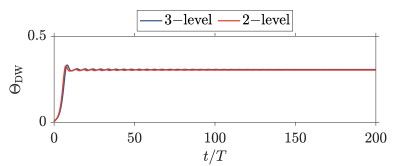
Figure 7: Dynamics of the density wave order parameter for $\omega_{\mathrm{dr}}=0.8\omega_{\mathrm{B}}$ and $f_{0}=0.05$. The remaining parameters are the same as in Fig. 6.

Appendix C Critical light-matter coupling

Using the Hamiltonian in Eq. (2) and the Heisenberg equation in Eq. (D13), we obtain the equations of motion as

$$\frac{da}{dt} =-(i\omega-\kappa)a-i\lambda_{12}\left(a^{\dagger}_{12}+a_{12}\right)-i\lambda_{13}\left(a^{\dagger}_{13}+a_{13}\right)$$ (C10)

$$\frac{da_{12}}{dt} =-i\omega_{12}a_{12}-i\lambda_{12}\left(a^{*}+a\right)$$

$$\frac{da_{13}}{dt} =-i\omega_{13}a_{13}-i\lambda_{13}\left(a^{*}+a\right)$$

We can then construct the matrix $M$ as $\partial_{t}\vec{v}=M\vec{v}$ to obtain

$$M=\left(\begin{array}[]{cccccc}\kappa-i\omega&0&-i\lambda_{12}&-i\lambda_{12}&-i\lambda_{13}&-i\lambda_{13}\\ 0&\kappa+i\omega&i\lambda_{12}&i\lambda_{12}&i\lambda_{13}&i\lambda_{13}\\ -i\lambda_{12}&-i\lambda_{12}&-i\omega_{12}&0&0&0\\ i\lambda_{12}&i\lambda_{12}&0&i\omega_{12}&0&0\\ -i\lambda_{13}&-i\lambda_{13}&0&0&-i\omega_{13}&0\\ i\lambda_{13}&i\lambda_{13}&0&0&0&i\omega_{13}\\ \end{array}\right)~{}.$$ (C11)

A phase transition occurs if $M$ inherits a zero energy eigenstate Kirton et al. (2019). This means, to find the critical light-matter coupling $\lambda$, we need to calculate $\mathrm{det}(M)=0$, giving us

$$\frac{\left(\kappa^{2}+\omega^{2}\right)}{4\omega}=\left(\frac{\lambda^{2}_{12}}{\omega_{12}}+\frac{\lambda^{2}_{13}}{\omega_{13}}\right).$$ (C12)

Appendix D Heisenberg Equations of Motion

The dynamics of an observable $\hat{O}$ in the dissipative system considered here is governed by the Heisenberg equation

$$\frac{d\langle\hat{O}\rangle}{dt}=\biggl{\langle}\frac{i}{\hbar}[\hat{H},\hat{O}]+\kappa\left(2\hat{a}^{\dagger}\hat{O}\hat{a}-\{\hat{a}^{\dagger}\hat{a},\hat{O}\}\right)\biggr{\rangle}.$$ (D13)

Using the commutation relations Eq. (A), we get the following equations for the expectation values of relevant operators in the open three-level Dicke model Eq. (1)

$$\frac{d\langle a\rangle}{dt} =-(i\omega+\kappa)\langle a\rangle-i\frac{2}{\sqrt{N}}\biggl{(}\lambda_{12}\langle\hat{J}^{12}_{x}\rangle+\lambda_{13}\langle\hat{J}^{13}_{x}\rangle\biggr{)}$$ (D14)

$$\frac{d\langle\hat{J}^{12}_{x}\rangle}{dt} =-\omega_{12}\langle\hat{J}^{12}_{y}\rangle+\frac{\lambda_{13}}{\sqrt{N}}\langle(a^{\dagger}+a)\hat{J}^{y}_{23}\rangle$$

$$\frac{d\langle\hat{J}^{12}_{y}\rangle}{dt} =\omega_{12}\langle\hat{J}^{12}_{x}\rangle-\frac{\lambda_{12}}{\sqrt{N}}\left(2\langle(a^{\dagger}+a)\hat{J}^{12}_{z}\rangle+\langle(a^{\dagger}+a)\hat{J}^{13}_{z}\rangle+\langle(a^{\dagger}+a)N/2\rangle\right)-\frac{\lambda_{13}}{\sqrt{N}}\langle(a^{\dagger}+a)\hat{J}^{23}_{x}\rangle$$

$$\frac{d\langle\hat{J}^{12}_{z}\rangle}{dt} =\frac{2\lambda_{12}}{\sqrt{N}}\langle(a+a^{\dagger})\hat{J}^{12}_{y}\rangle$$

$$\frac{d\langle\hat{J}^{13}_{x}\rangle}{dt} =-\omega_{13}\langle\hat{J}^{13}_{y}\rangle-\frac{\lambda_{12}}{\sqrt{N}}\langle(a^{\dagger}+a)\hat{J}^{23}_{y}\rangle$$

$$\frac{d\langle\hat{J}^{13}_{y}\rangle}{dt} =\omega_{13}\langle\hat{J}^{13}_{x}\rangle-\frac{\lambda_{13}}{\sqrt{N}}\left(2\langle(a^{\dagger}+a)\hat{J}^{13}_{z}\rangle+\langle(a^{\dagger}+a)\hat{J}^{12}_{z}\rangle+\langle(a^{\dagger}+a)N/2\rangle\right)-\frac{\lambda_{12}}{\sqrt{N}}\langle(a^{\dagger}+a)\hat{J}^{23}_{x}\rangle$$

$$\frac{d\langle\hat{J}^{13}_{z}\rangle}{dt} =\frac{2\lambda_{13}}{\sqrt{N}}\langle(a+a^{\dagger})\hat{J}^{13}_{y}\rangle$$

$$\frac{d\langle\hat{J}^{23}_{x}\rangle}{dt} =(\omega_{13}-\omega_{12})\langle\hat{J}^{23}_{y}\rangle+\frac{\lambda_{12}}{\sqrt{N}}\langle(a^{\dagger}+a)\hat{J}^{13}_{y}\rangle+\frac{\lambda_{13}}{\sqrt{N}}\langle(a^{\dagger}+a)\hat{J}^{12}_{y}\rangle$$

$$\frac{d\langle\hat{J}^{23}_{y}\rangle}{dt} =(\omega_{12}-\omega_{13})\langle\hat{J}^{23}_{y}\rangle+\frac{\lambda_{12}}{\sqrt{N}}\langle(a^{\dagger}+a)\hat{J}^{13}_{x}\rangle-\frac{\lambda_{13}}{\sqrt{N}}\langle(a^{\dagger}+a)\hat{J}^{12}_{x}\rangle$$

On the other hand, the equations of motion for the parametrically driven open three-level Dicke model are

$$\frac{d\langle\hat{a}\rangle}{dt} =-(i\omega+\kappa)\langle\hat{a}\rangle-i\frac{2\lambda}{\sqrt{N}}\langle\hat{J}^{\mathrm{D}}_{x}\rangle+i\phi(t)\frac{2\lambda}{\sqrt{N}}\langle\hat{J}^{\mathrm{B}}_{x}\rangle$$ (D15)

$$\frac{d\langle\hat{J}^{\mathrm{D}}_{x}\rangle}{dt} =-\omega_{\mathrm{D}}\langle\hat{J}^{\mathrm{D}}_{y}\rangle-\phi(t)(\omega_{\mathrm{B}}-\omega_{\mathrm{D}})\langle\hat{J}^{\mathrm{B}}_{y}\rangle-\phi(t)\frac{\lambda}{\sqrt{N}}\langle(a^{\dagger}+a)\hat{J}^{\mathrm{DB}}_{y}\rangle$$

$$\frac{d\langle\hat{J}^{\mathrm{D}}_{y}\rangle}{dt} =\omega_{\mathrm{D}}\langle\hat{J}^{\mathrm{D}}_{x}\rangle-\frac{\lambda}{\sqrt{N}}\biggl{[}2\langle(a^{\dagger}+a)\hat{J}^{\mathrm{D}}_{z}\rangle+\langle(a^{\dagger}+a)\hat{J}^{\mathrm{B}}_{z}\rangle+\langle a^{\dagger}+a\rangle\frac{N}{2}\biggr{]}+\phi(t)(\omega_{\mathrm{B}}-\omega_{\mathrm{D}})\langle\hat{J}^{\mathrm{B}}_{x}\rangle+\phi(t)\frac{\lambda}{\sqrt{N}}\langle(a^{\dagger}+a)\hat{J}^{\mathrm{DB}}_{x}\rangle$$

$$\frac{d\langle\hat{J}^{\mathrm{D}}_{z}\rangle}{dt} =\frac{2\lambda}{\sqrt{N}}\langle(a+a^{\dagger})\hat{J}^{\mathrm{D}}_{y}\rangle+2(\omega_{\mathrm{B}}-\omega_{\mathrm{D}})\phi(t)\langle\hat{J}^{\mathrm{DB}}_{y}\rangle$$

$$\frac{d\langle\hat{J}^{\mathrm{B}}_{x}\rangle}{dt} =-\omega_{\mathrm{B}}\langle\hat{J}^{\mathrm{B}}_{y}\rangle-\phi(t)(\omega_{\mathrm{B}}-\omega_{\mathrm{D}})\langle\hat{J}^{\mathrm{D}}_{y}\rangle-\frac{\lambda}{\sqrt{N}}\langle(a^{\dagger}+a)\hat{J}^{\mathrm{DB}}_{y}\rangle$$

$$\frac{d\langle\hat{J}^{\mathrm{B}}_{y}\rangle}{dt} =\omega_{\mathrm{B}}\langle\hat{J}^{\mathrm{B}}_{x}\rangle+\phi(t)\frac{\lambda}{\sqrt{N}}\biggl{[}2\langle(a^{\dagger}+a)\hat{J}^{\mathrm{B}}_{z}\rangle+\langle(a^{\dagger}+a)\hat{J}^{\mathrm{D}}_{z}\rangle+\langle a^{\dagger}+a\rangle\frac{N}{2}\biggr{]}+\phi(t)(\omega_{\mathrm{B}}-\omega_{\mathrm{D}})\langle\hat{J}^{\mathrm{D}}_{x}\rangle-\frac{\lambda}{\sqrt{N}}\langle(a^{\dagger}+a)\hat{J}^{\mathrm{DB}}_{x}\rangle$$

$$\frac{d\langle\hat{J}^{\mathrm{B}}_{z}\rangle}{dt} =-\phi(t)(\omega_{\mathrm{B}}-\omega_{\mathrm{D}})\langle(a+a^{\dagger})\hat{J}^{\mathrm{B}}_{y}\rangle-\frac{4\lambda^{2}}{U_{0}N}\phi(t)\langle\hat{J}^{\mathrm{DB}}_{y}\rangle$$

$$\frac{d\langle\hat{J}^{\mathrm{DB}}_{x}\rangle}{dt} =(\omega_{\mathrm{B}}-\omega_{\mathrm{D}})\langle\hat{J}^{\mathrm{DB}}_{y}\rangle+\frac{\lambda}{\sqrt{N}}\langle(a^{\dagger}+a)\hat{J}^{\mathrm{B}}_{y}\rangle-\phi(t)\frac{\lambda}{\sqrt{N}}\langle(a^{\dagger}+a)\hat{J}^{\mathrm{D}}_{y}\rangle$$

$$\frac{d\langle\hat{J}^{\mathrm{DB}}_{y}\rangle}{dt} =(\omega_{\mathrm{D}}-\omega_{\mathrm{B}})\langle\hat{J}^{\mathrm{DB}}_{x}\rangle+\frac{\lambda}{\sqrt{N}}\langle(a^{\dagger}+a)\hat{J}^{\mathrm{B}}_{x}\rangle+\phi(t)\frac{\lambda}{\sqrt{N}}\langle(a^{\dagger}+a)\hat{J}^{\mathrm{D}}_{x}\rangle+2(\omega_{\mathrm{B}}-\omega_{\mathrm{D}})\phi(t)\langle\hat{J}^{\mathrm{B}}_{z}-\hat{J}^{\mathrm{D}}_{z}\rangle$$

Appendix E Mean-field equations of motion

The mean-field equations for the dissipative three-level Dicke model are given by

$$\frac{da}{dt} =-(i\omega+\kappa)a-i2\lambda_{12}j^{12}_{x}-i2\lambda_{13}j^{13}_{x}$$ (E16)

$$\frac{dj^{12}_{x}}{dt} =-\omega_{12}j^{12}_{y}+\lambda_{13}(a+a^{*})j^{y}_{23}$$

$$\frac{dj^{12}_{y}}{dt} =\omega_{12}j^{12}_{x}-\lambda_{12}(a+a^{*})\left(2j^{12}_{z}+j^{13}_{z}+1/2\right)$$

$$\qquad-\lambda_{13}(a+a^{*})j^{23}_{x}$$

$$\frac{dj^{12}_{z}}{dt} =2\lambda_{12}(a+a^{*})j^{12}_{y}$$

$$\frac{dj^{13}_{x}}{dt} =-\omega_{13}j^{13}_{y}-\lambda_{12}(a+a^{*})j^{23}_{y}$$

$$\frac{dj^{13}_{y}}{dt} =\omega_{13}j^{13}_{x}-\lambda_{13}(a+a^{*})\left(2j^{13}_{z}+j^{12}_{z}+1/2\right)$$

$$\qquad-\lambda_{12}(a+a^{*})j^{23}_{x}$$

$$\frac{dj^{13}_{z}}{dt} =2\lambda_{13}(a+a^{*})j^{13}_{y}$$

$$\frac{dj^{23}_{x}}{dt} =(\omega_{13}-\omega_{12})j^{23}_{y}+\lambda_{12}(a+a^{*})j^{13}_{y}+\lambda_{13}(a+a^{*})j^{12}_{y}$$

$$\frac{dj^{23}_{y}}{dt} =(\omega_{12}-\omega_{13})j^{23}_{y}+\lambda_{12}(a+a^{*})j^{13}_{x}-\lambda_{13}(a+a^{*})j^{12}_{x}$$

For the parametrically driven open three-level Dicke model, the equations of motion are given by

$$\frac{da}{dt} =-(i\omega+\kappa)a-i2\lambda j^{\mathrm{D}}_{x}+i\phi(t)2\lambda j^{\mathrm{B}}_{x}$$ (E17)

$$\frac{dj^{\mathrm{D}}_{x}}{dt} =-\omega_{\mathrm{D}}j^{\mathrm{D}}_{y}-\phi(t)(\omega_{\mathrm{B}}-\omega_{\mathrm{D}})j^{\mathrm{B}}_{y}-\phi(t)\lambda(a+a^{*})j^{\mathrm{DB}}_{y}$$

$$\frac{dj^{\mathrm{D}}_{y}}{dt} =\omega_{\mathrm{D}}j^{\mathrm{D}}_{x}-\lambda(a+a^{*})\biggl{(}2j^{\mathrm{D}}_{z}+j^{\mathrm{B}}_{z}+1/2\biggr{)}$$

$$\qquad+\phi(t)(\omega_{\mathrm{B}}-\omega_{\mathrm{D}})j^{\mathrm{B}}_{x}+\phi(t)\lambda(a+a^{*})j^{\mathrm{DB}}_{x}$$

$$\frac{dj^{\mathrm{D}}_{z}}{dt} =2\lambda(a+a^{*})j^{\mathrm{D}}_{y}+2(\omega_{\mathrm{B}}-\omega_{\mathrm{D}})\phi(t)j^{\mathrm{DB}}_{y}$$

$$\frac{dj^{\mathrm{B}}_{x}}{dt} =-\omega_{\mathrm{B}}j^{\mathrm{B}}_{y}-(\omega_{\mathrm{B}}-\omega_{\mathrm{D}})\phi(t)j^{\mathrm{D}}_{y}-\lambda(a+a^{*})j^{\mathrm{DB}}_{y}$$

$$\frac{dj^{\mathrm{B}}_{y}}{dt} =\omega_{\mathrm{B}}j^{\mathrm{B}}_{x}+\phi(t)\lambda(a+a^{*})\biggl{(}2j^{\mathrm{B}}_{z}+j^{\mathrm{D}}_{z}+1/2\biggr{)}$$

$$\qquad+\phi(t)(\omega_{\mathrm{B}}-\omega_{\mathrm{D}})j^{\mathrm{D}}_{x}-\lambda(a+a^{*})j^{\mathrm{DB}}_{x}$$

$$\frac{dj^{\mathrm{B}}_{z}}{dt} =-\phi(t)2\lambda(a+a^{*})j^{\mathrm{B}}_{y}-2(\omega_{\mathrm{B}}-\omega_{\mathrm{D}})\phi(t)j^{\mathrm{DB}}_{y}$$

$$\frac{dj^{\mathrm{DB}}_{x}}{dt} =(\omega_{\mathrm{B}}-\omega_{\mathrm{D}})j^{\mathrm{DB}}_{y}+\lambda(a+a^{*})j^{\mathrm{B}}_{y}-\phi(t)\lambda(a+a^{*})j^{\mathrm{D}}_{y}$$

$$\frac{dj^{\mathrm{DB}}_{y}}{dt} =(\omega_{\mathrm{D}}-\omega_{\mathrm{B}})j^{\mathrm{DB}}_{x}+\lambda(a+a^{*})j^{\mathrm{B}}_{x}+\phi(t)\lambda(a+a^{*})j^{\mathrm{D}}_{x}$$

$$\qquad+2(\omega_{\mathrm{B}}-\omega_{\mathrm{D}})\phi(t)(j^{\mathrm{B}}_{z}-j^{\mathrm{D}}_{z}).$$

In Fig. 8, we demonstrate that the existence of the dynamical phases is independent of the term in the Hamiltonian with $j^{\mathrm{DB}}_{x}$. That is, the momenta coupling inferred from Eq. (5) does not play a crucial role in the formation of the ITC, LESR, and LISR phases. This suggests that the emergence of these dynamical phases originates from the last term in Eq. (4). To confirm this, we set $\omega_{\mathrm{D}}=\omega_{\mathrm{B}}$ in Fig. 8. For comparison, we show in dotted lines the phase boundary obtained for $\omega_{\mathrm{D}}\neq\omega_{\mathrm{B}}$.

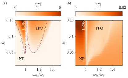
Figure 8: Time-averaged cavity mode occupation $|a|^{2}$ taken over 100 driving cycles, $\tau=100T$. We choose $\omega_{\mathrm{D}}=\omega_{\mathrm{B}}=\omega_{\mathrm{rec}}$ while the remaining parameters are the same as those in Figs. 5(a)-(b).

Appendix F Holstein-Primakoff Transformation

We present a Holstein-Primakoff approximation in the thermodynamic limit, i.e. $N\rightarrow\infty$ Emary and Brandes (2003); Bastidas et al. (2012). To capture the correct SU(3) algebra, we use an extended version of the Holstein-Primakoff representation given by Wagner (1975)

$$\hat{J}^{12}_{z} =\hat{a}^{\dagger}_{12}\hat{a}_{12}-N/2,\quad\hat{J}^{12}_{+}=\hat{a}^{\dagger}_{12}~{}\sqrt{N-\left(\hat{a}^{\dagger}_{12}\hat{a}_{12}+\hat{a}^{\dagger}_{13}\hat{a}_{13}\right)}$$ (F18)

$$\hat{J}^{12}_{-} =\sqrt{N-\left(\hat{a}^{\dagger}_{12}\hat{a}_{12}+\hat{a}^{\dagger}_{13}\hat{a}_{13}\right)}~{}\hat{a}_{12}$$

$$\hat{J}^{13}_{z} =\hat{a}^{\dagger}_{13}\hat{a}_{13}-N/2,\quad\hat{J}^{13}_{+}=\hat{a}^{\dagger}_{13}~{}\sqrt{N-\left(\hat{a}^{\dagger}_{12}\hat{a}_{12}+\hat{a}^{\dagger}_{13}\hat{a}_{13}\right)}$$

$$\hat{J}^{13}_{-} =\sqrt{N-\left(\hat{a}^{\dagger}_{12}\hat{a}_{12}+\hat{a}^{\dagger}_{13}\hat{a}_{13}\right)}~{}\hat{a}_{13}$$

$$\hat{J}^{23}_{+} =\hat{a}^{\dagger}_{12}\hat{a}_{13},\quad\hat{J}^{23}_{-}=\hat{a}^{\dagger}_{13}\hat{a}_{12}.$$

In the $N\to\infty$ limit, we can further approximate the pseudospin operators as

$$\hat{J}^{\mathrm{D}}_{z} =\hat{a}^{\dagger}_{12}\hat{a}_{12}-N/2,\quad\hat{J}^{\mathrm{D}}_{+}=\hat{a}^{\dagger}_{12}~{}\sqrt{N},\quad\hat{J}^{\mathrm{D}}_{-}=\sqrt{N}~{}\hat{a}_{12}$$ (F19)

$$\hat{J}^{\mathrm{B}}_{z} =\hat{a}^{\dagger}_{13}\hat{a}_{13}-N/2,\quad\hat{J}^{\mathrm{B}}_{+}=\hat{a}^{\dagger}_{13}~{}\sqrt{N},\quad\hat{J}^{\mathrm{B}}_{-}=\sqrt{N}~{}\hat{a}_{13}$$

$$\hat{J}^{\mathrm{DB}}_{+} =\hat{a}^{\dagger}_{12}\hat{a}_{13},\qquad\hat{J}^{\mathrm{DB}}_{-}=\hat{a}^{\dagger}_{13}\hat{a}_{12}.$$

In an analogue fashion for the driven three-level Dicke model we obtain the Hamiltonian with $a_{12}\rightarrow d$ and $a_{13}\rightarrow b$

$$H/\hbar =\omega\hat{a}^{\dagger}\hat{a}+\omega_{\mathrm{D}}\hat{d}^{\dagger}\hat{d}+\omega_{\mathrm{B}}\hat{b}^{\dagger}\hat{b}+\lambda\left(\hat{a}^{\dagger}+\hat{a}\right)$$ (F20)

$$\qquad\times\left[(\hat{d}^{\dagger}+\hat{d})-\phi(t)(\hat{b}^{\dagger}+\hat{b})\right]$$

$$\qquad+\phi(t)(\omega_{\mathrm{B}}-\omega_{\mathrm{D}})\left(\hat{d}^{\dagger}\hat{b}+\hat{b}^{\dagger}\hat{d}\right)~{}.$$

The mean-field equations of motion for Eq. (F20) are

$$\frac{\partial a}{\partial t} =-(i\omega-\kappa)a-i\lambda(d^{*}+d)+i\phi(t)\lambda({b}^{*}+{b})$$ (F21)

$$\frac{\partial d}{\partial t} =-i\omega_{\mathrm{D}}d-i\lambda(a^{*}+a)-i(\omega_{\mathrm{B}}-\omega_{\mathrm{D}})\phi(t)b.$$

$$\frac{\partial b}{\partial t} =-i\omega_{\mathrm{B}}b+i\phi(t)\lambda({a}^{*}+{a})-i(\omega_{\mathrm{B}}-\omega_{\mathrm{D}})\phi(t)d.$$

Appendix G Lower Polariton

Consider the standard closed Dicke model

$$\hat{H}/\hbar=\omega\hat{a}^{\dagger}\hat{a}+\omega_{0}\hat{J}_{z}+\frac{2\lambda}{\sqrt{N}}(\hat{a}^{\dagger}+\hat{a})(\hat{J}_{x}).$$ (G22)

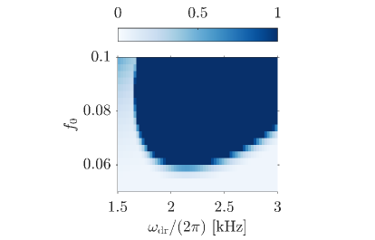
Figure 9: Maximum value of $(b+b^{*})$. The parameters are the same as those in Figs. 3(a)-(d).

In the thermodynamic limit, this can be diagonalised using the Holstein-Primakoff transformation, which leads to two polariton frequencies

$$\omega_{\mathrm{LP},\kappa=0}=\biggl{(}\frac{(\omega^{2}_{0}+\omega^{2})}{2}-\frac{1}{2}\sqrt{(\omega^{2}_{0}-\omega^{2})^{2}+16\lambda^{2}\omega\omega_{0}}\biggr{)}^{1/2}$$ (G23)

$$\omega_{\mathrm{UP},\kappa=0}=\biggl{(}\frac{(\omega^{2}_{0}+\omega^{2})}{2}+\frac{1}{2}\sqrt{(\omega^{2}_{0}-\omega^{2})^{2}+16\lambda^{2}\omega\omega_{0}}\biggr{)}^{1/2}.$$ (G24)

The lower polariton frequency, Eq. (G23), is the upper bound in the presence of dissipation. When $\kappa\neq 0$, the lower polariton frequency can be numerically determined by exploiting the parametric resonance when the light-matter coupling is periodically driven Bastidas et al. (2012); Chitra and Zilberberg (2015)

$$\lambda(t)=\lambda_{0}(1+f_{0}\sin(\omega_{dr}t)).$$ (G25)

In the limit $N\to\infty$, the Hamiltonian can be reduced to a coupled oscillator, whereby the coupling strength is periodic in time. This possesses a parametric resonance manifesting as a resonance lobe centred at the primary resonance, $\omega_{\mathrm{dr}}=2\omega_{\mathrm{LP}}$. Thus, we can determine $\omega_{\mathrm{LP}}$ by mapping the instability region for varying modulation parameters $f_{0}$ and $\omega_{\mathrm{dr}}$. To this end, we solve the corresponding equations of motion given by

$$i\frac{\partial a}{\partial t} =(\omega-i\kappa)a+\lambda(t)(b^{*}+b)$$ (G26)

$$i\frac{\partial b}{\partial t} =\omega_{0}b+\lambda(t)(a^{*}+a)$$

The unstable region indicating the parametric resonance is signalled by a diverging $(b+b^{*})$, as depicted in Fig. 9. We obtain a lower polariton frequency $\omega_{\mathrm{LP}}/2\pi\approx 1.06~{}\mathrm{kHz}$, which is the value used in the sum frequency condition denoted by the vertical line in Figs. 3(a)-(d).

Appendix H Parameters

We consider realistic parameters based on the experimental setup in Ref. joi . A BEC of $N=65\times 10^{3}$ ⁸⁷Rb atoms is coupled to a high-finesse optical cavity with a photon loss rate of $\kappa=~{}2\pi\times 3.6~{}\mathrm{kHz}$. This is very close to the recoil frequency, $\omega_{\mathrm{rec}}=2\pi\times 3.55~{}\mathrm{kHz}$, associated with the standing wave potential of the pump. The cavity light shift per atom is $U_{0}=-2\pi\times 0.36~{}\mathrm{Hz}$. The effective pump-cavity detuning is fixed to $\delta_{\mathrm{eff}}=-2\pi\times 18.5~{}\mathrm{kHz}$. We are interested in the two regimes $\lambda<\lambda_{\mathrm{cr}}$ and $\lambda>\lambda_{\mathrm{cr}}$, where $\lambda_{\mathrm{cr}}$ is the critical light-matter coupling strength needed to enter the DW phase in the absence of modulation, where $\lambda_{\mathrm{cr}}=\sqrt{(\kappa^{2}+\omega^{2})\left(\omega_{\mathrm{D}}/\omega\right)}/2$. By equating the expression for $\lambda_{\mathrm{cr}}$ and $\lambda$ in terms of the atom-cavity parameters for the two-level Dicke model, we find that the critical pump strength is given by $\epsilon_{\mathrm{cr}}={8(\omega^{2}+\kappa^{2})}/{\left(4N\omega|\Delta_{0}|+{(\omega^{2}+\kappa^{2})}\right)}$.

References

- Dicke (1954) R. H. Dicke, “Coherence in spontaneous radiation processes,” Phys. Rev. 93, 99–110 (1954).
- Baumann et al. (2010) K. Baumann, C. Guerlin, F. Brennecke, and T. Esslinger, “Dicke quantum phase transition with a superfluid gas in an optical cavity,” Nature 464, 1301–1306 (2010).
- Klinder et al. (2015) J. Klinder, H. Keßler, M. Wolke, L. Mathey, and A. Hemmerich, “Dynamical phase transition in the open Dicke model,” Proc. Natl. Acad. Sci. USA 112, 3290–3295 (2015).
- Hayn et al. (2011) M. Hayn, C. Emary, and T. Brandes, “Phase transitions and dark-state physics in two-color superradiance,” Phys. Rev. A 84, 053856 (2011).
- Bastidas et al. (2012) V. M. Bastidas, C. Emary, B. Regler, and T. Brandes, “Nonequilibrium quantum phase transitions in the dicke model,” Phys. Rev. Lett. 108, 043003 (2012).
- Chitra and Zilberberg (2015) R. Chitra and O. Zilberberg, “Dynamical many-body phases of the parametrically driven, dissipative Dicke model,” Phys. Rev. A 92, 023815 (2015).
- Zhiqiang et al. (2017) Z. Zhiqiang, C. H. Lee, R. Kumar, K. J. Arnold, S. J. Masson, A. S. Parkins, and M. D. Barrett, “Nonequilibrium phase transition in a spin-1 Dicke model,” Optica 4, 424 (2017).
- Soriente et al. (2018) M. Soriente, T. Donner, R. Chitra, and O. Zilberberg, “Dissipation-Induced Anomalous Multicritical Phenomena,” Phys. Rev. Lett. 120, 183603 (2018).
- Chiacchio and Nunnenkamp (2019) E. I. R. Chiacchio and A. Nunnenkamp, “Dissipation-induced instabilities of a spinor bose-einstein condensate inside an optical cavity,” Phys. Rev. Lett. 122, 193605 (2019).
- Buča and Jaksch (2019) B. Buča and D. Jaksch, “Dissipation induced nonstationarity in a quantum gas,” Phys. Rev. Lett. 123, 260401 (2019).
- Stitely et al. (2020) K. C. Stitely, S. J. Masson, A. Giraldo, B. Krauskopf, and S. Parkins, “Superradiant switching, quantum hysteresis, and oscillations in a generalized Dicke model,” Phys. Rev. A 102, 063702 (2020).
- Habibian et al. (2013) H. Habibian, A. Winter, S. Paganelli, H. Rieger, and G. Morigi, “Bose-Glass Phases of Ultracold Atoms due to Cavity Backaction,” Phys. Rev. Lett. 110, 075304 (2013).
- Kollath et al. (2016) C. Kollath, A. Sheikhan, S. Wolff, and F. Brennecke, “Ultracold Fermions in a Cavity-Induced Artificial Magnetic Field,” Phys. Rev. Lett. 116, 060401 (2016).
- Mivehvar et al. (2017) F. Mivehvar, F. Piazza, and H. Ritsch, “Disorder-Driven Density and Spin Self-Ordering of a Bose-Einstein Condensate in a Cavity,” Phys. Rev. Lett. 119, 063602 (2017).
- Vaidya et al. (2018) V. D. Vaidya, Y. Guo, R. M. Kroeze, K. E. Ballantine, A. J. Kollár, J. Keeling, and B. L. Lev, “Tunable-Range, Photon-Mediated Atomic Interactions in Multimode Cavity QED,” Physical Review X 8, 011002 (2018).
- Landini et al. (2018) M. Landini, N. Dogra, K. Kroeger, L. Hruby, T. Donner, and T. Esslinger, “Formation of a spin texture in a quantum gas coupled to a cavity,” Phys. Rev. Lett. 120, 223602 (2018).
- Dogra et al. (2019) N. Dogra, M. Landini, K. Kroeger, L. Hruby, T. Donner, and T. Esslinger, “Dissipation-induced structural instability and chiral dynamics in a quantum gas,” Science 366, 1496–1499 (2019).
- Bentsen et al. (2019) G. Bentsen, I.-D. Potirniche, V. B. Bulchandani, T. Scaffidi, X. Cao, X.-L. Qi, M. Schleier-Smith, and E. Altman, “Integrable and Chaotic Dynamics of Spins Coupled to an Optical Cavity,” Phys. Rev. X 9, 041011 (2019).
- Jäger et al. (2020) S. B. Jäger, M. J. Holland, and G. Morigi, “Superradiant optomechanical phases of cold atomic gases in optical resonators,” Phys. Rev. A 101, 023616 (2020).
- Boller et al. (1991) K.-J. Boller, A. Imamoğlu, and S. E. Harris, “Observation of electromagnetically induced transparency,” Phys. Rev. Lett. 66, 2593–2596 (1991).
- Fleischhauer et al. (2005) M. Fleischhauer, A. Imamoglu, and J. P. Marangos, “Electromagnetically induced transparency: Optics in coherent media,” Rev. Mod. Phys. 77, 633–673 (2005).
- Scully et al. (1989) M. O. Scully, S.-Y. Zhu, and A. Gavrielides, “Degenerate quantum-beat laser: Lasing without inversion and inversion without lasing,” Phys. Rev. Lett. 62, 2813–2816 (1989).
- Mompart and Corbalán (2000) J Mompart and R Corbalán, “Lasing without inversion,” J. Opt. B: Quantum Semiclass. Opt. 2, R7–R24 (2000).
- Gaubatz et al. (1990) U. Gaubatz, P. Rudecki, S. Schiemann, and K. Bergmann, “Population transfer between molecular vibrational levels by stimulated raman scattering with partially overlapping laser fields. a new concept and experimental results,” J. Chem. Phys 92, 5363–5376 (1990).
- Vitanov et al. (2017) N. V. Vitanov, A. A. Rangelov, B. W. Shore, and K. Bergmann, “Stimulated raman adiabatic passage in physics, chemistry, and beyond,” Rev. Mod. Phys. 89, 015006 (2017).
- Sung and Bowden (1979) C. C. Sung and C. M. Bowden, “Phase transition in the multimode two- and three-level Dicke model (Green’s function method),” J. Phys. A: Math. Gen. 12, 2273 (1979).
- Crubellier et al. (1985) A. Crubellier, S. Liberman, D. Pavolini, and P. Pillet, “Superradiance and subradiance. I. Interatomic interference and symmetry properties in three-level systems,” J. Phys. B: At. Mol. Phys. 18, 3811–3833 (1985).
- Crubellier and Pavolini (1986) A. Crubellier and D. Pavolini, “Superradiance and subradiance. II. Atomic systems with degenerate transitions,” J. Phys. B: At. Mol. Phys. 19, 2109–2138 (1986).
- Cola et al. (2009) M. M. Cola, D. Bigerni, and N. Piovella, “Recoil-induced subradiance in an ultracold atomic gas,” Phys. Rev. A 79, 053622 (2009).
- Wolf et al. (2018) P. Wolf, S. C. Schuster, D. Schmidt, S. Slama, and C. Zimmermann, “Observation of Subradiant Atomic Momentum States with Bose-Einstein Condensates in a Recoil Resolving Optical Ring Resonator,” Phys. Rev. Lett. 121, 173602 (2018).
- Georgi (2018) H. Georgi, Lie Algebras In Particle Physics: from Isospin To Unified Theories (CRC Press, 2018).
- Marciano and Pagels (1978) W. Marciano and H. Pagels, “Quantum chromodynamics,” Physics Reports 36, 137–276 (1978).
- Griffiths (2008) D. Griffiths, Introduction to elementary particles (2008).
- Cosme et al. (2019) J. G. Cosme, J. Skulte, and L. Mathey, “Time crystals in a shaken atom-cavity system,” Phys. Rev. A 100, 053615 (2019).
- (35) See P. Kongkhambut et al. for details.
- Sakurai and Napolitano (2017) J. J. Sakurai and Jim Napolitano, Modern Quantum Mechanics, 2nd ed. (Cambridge University Press, 2017).
- Baksic et al. (2013) A. Baksic, P. Nataf, and C. Ciuti, “Superradiant phase transitions with three-level systems,” Phys. Rev. A 87, 023813 (2013).
- Dimer et al. (2007) F. Dimer, B. Estienne, A. S. Parkins, and H. J. Carmichael, “Proposed realization of the dicke-model quantum phase transition in an optical cavity qed system,” Phys. Rev. A 75, 013804 (2007).
- Kirton et al. (2019) P. Kirton, M. M. Roses, J. Keeling, and E. G. Dalla Torre, “Introduction to the Dicke Model: From Equilibrium to Nonequilibrium, and Vice Versa,” Adv. Quantum Technol. 2, 1800043 (2019).
- Mivehvar et al. (2021) F. Mivehvar, F. Piazza, T. Donner, and H. Ritsch, “Cavity QED with Quantum Gases: New Paradigms in Many-Body Physics,” arXiv e-prints , arXiv:2102.04473 (2021), arXiv:2102.04473 .
- Ritsch et al. (2013) H. Ritsch, P. Domokos, F. Brennecke, and T. Esslinger, “Cold atoms in cavity-generated dynamical optical potentials,” Rev. Mod. Phys. 85, 553–601 (2013).
- Cosme et al. (2018) J. G. Cosme, C. Georges, A. Hemmerich, and L. Mathey, “Dynamical Control of Order in a Cavity-BEC System,” Phys. Rev. Lett. 121, 153001 (2018).
- Georges et al. (2018) C. Georges, J. G. Cosme, L. Mathey, and A. Hemmerich, “Light-Induced Coherence in an Atom-Cavity System,” Phys. Rev. Lett. 121, 220405 (2018).
- Keßler et al. (2019) H. Keßler, J. G. Cosme, M. Hemmerling, L. Mathey, and A. Hemmerich, “Emergent limit cycles and time crystal dynamics in an atom-cavity system,” Phys. Rev. A 99, 053605 (2019).
- Keßler et al. (2020) H. Keßler, J. G. Cosme, C. Georges, L. Mathey, and A. Hemmerich, “From a continuous to a discrete time crystal in a dissipative atom-cavity system,” New J. Phys. 22, 085002 (2020).
- Keßler et al. (2021) H. Keßler, P. Kongkhambut, C. Georges, L. Mathey, J. G. Cosme, and A. Hemmerich, “Observation of a Dissipative Time Crystal,” Phys. Rev. Lett. 127, 043602 (2021).
- Georges et al. (2021) C. Georges, J. G. Cosme, H. Keßler, L. Mathey, and A. Hemmerich, “Dynamical density wave order in an atom-cavity system,” New J. Phys. 23, 023003 (2021).
- Fausti et al. (2011) D. Fausti, R. I. Tobey, N. Dean, S. Kaiser, A. Dienst, M. C. Hoffmann, S. Pyon, T. Takayama, H. Takagi, and A. Cavalleri, “Light-Induced Superconductivity in a Stripe-Ordered Cuprate,” Science 331, 189 (2011).
- Hu et al. (2014) W. Hu, S. Kaiser, D. Nicoletti, C. R. Hunt, I. Gierz, M. C. Hoffmann, M. Le Tacon, T. Loew, B. Keimer, and A. Cavalleri, “Optically enhanced coherent transport in YBa2Cu3O6.5 by ultrafast redistribution of interlayer coupling,” Nat. Mater. 13, 705–711 (2014).
- Mankowsky et al. (2014) R. Mankowsky, A. Subedi, M. Först, S. O. Mariager, M. Chollet, H. T. Lemke, J. S. Robinson, J. M. Glownia, M. P. Minitti, A. Frano, M. Fechner, N. A. Spaldin, T. Loew, B. Keimer, A. Georges, and A. Cavalleri, “Nonlinear lattice dynamics as a basis for enhanced superconductivity in ,” Nature 516, 71–73 (2014).
- Denny et al. (2015) S. J. Denny, S. R. Clark, Y. Laplace, A. Cavalleri, and D. Jaksch, “Proposed parametric cooling of bilayer cuprate superconductors by terahertz excitation,” Phys. Rev. Lett. 114, 137001 (2015).
- Okamoto et al. (2016) J.-i. Okamoto, A. Cavalleri, and L. Mathey, “Theory of enhanced interlayer tunneling in optically driven high- superconductors,” Phys. Rev. Lett. 117, 227001 (2016).
- Homann et al. (2021) G. Homann, J. G. Cosme, J. Okamoto, and L. Mathey, “Higgs mode mediated enhancement of interlayer transport in high- cuprate superconductors,” Phys. Rev. B 103, 224503 (2021).
- Homann et al. (2020) G. Homann, J. G. Cosme, and L. Mathey, “Higgs time crystal in a high- superconductor,” Phys. Rev. Research 2, 043214 (2020).
- Lin et al. (2021) R. Lin, R. Rosa-Medina, F. Ferri, F. Finger, K. Kroeger, T. Donner, T. Esslinger, and R. Chitra, “Dissipation-engineered family of nearly dark states in many-body cavity-atom systems,” (2021), arXiv:2109.00422 [cond-mat.quant-gas] .
- Emary and Brandes (2003) C. Emary and T. Brandes, “Chaos and the quantum phase transition in the dicke model,” Phys. Rev. E 67, 066203 (2003).
- Wagner (1975) M. Wagner, “A nonlinear transformation of SU(3)-spin-operators to bosonic operators,” Physics Letters A 53, 1–2 (1975).