1 Introduction

The discovery of a Higgs boson with a mass of approximately $125\ \mathrm{GeV}$ at the LHC by both the ATLAS [1] and the CMS [2] collaborations is a milestone for the understanding of the laws of nature. So far, the experimental observation related to the discovered particle, denoted by $h_{125}$ in the following, agree with the interpretation of a fundamental scalar particle that behaves according to the prediction of the Standard Model (SM) [3, 4, 5]. As a result, any model has to incorporate a particle state that resembles a SM-like Higgs boson within the current experimental uncertainties. In contrast to the measurement of the Higgs-boson mass, the measurements of the couplings of $h_{125}$ are much less precise, with uncertainties at the level of about ten to twenty percent [4, 5]. This leaves room for interpretations of the discovered Higgs boson in models beyond the SM (BSM), in which the theoretical predictions of the properties of $h_{125}$ only agree with the SM interpretation at the level of the current experimental uncertainties. In such models, phenomena can be accommodated that cannot be explained in the SM, and the precise measurements of the properties of $h_{125}$ will be crucial in order to shed light on the question which of the proposed BSM scenarios could be realized in nature.

Another experimental milestone consists of various indications for the existence of dark matter (DM) through a conjoint of data gathered from, among others, rotation curves of spatial galaxies [6, 7], gravitational lensing [8], and the Bullet cluster merger [9]. The Planck collaboration [10], using the precise map of the cosmic microwave background (CMB), reports the most precise measurement of today’s DM relic abundance, ${(\Omega h^{2})_{\rm Planck}=(0.119\pm 0.003)}$. Hence, the DM sector constitutes about $26\%$ of the energy-matter content of the Universe. Even though there are many indirect indications for the existence of DM via gravitational effects, so far there has not been any direct discovery of a DM particle that could give rise to more information about the properties of DM. The elusive nature of DM has opened up an interesting landscape of BSM theories that can provide one or more DM candidates. One of the most studied scenarios in such SM extensions is the weakly-interacting particle (WIMP), a particle with weak couplings to the SM particles and a mass around the electroweak (EW) scale whose existence could potentially be probed also at present or future colliders. In view of the fact that the DM particle(s) might not be charged under the SM gauge groups, in which case they are also not coupled directly to the quarks and leptons, the possibility of coupling the DM to the SM only via the Higgs sector, often called Higgs portal [11, 12], is an interesting scenario. Many extended Higgs sectors provide a (pseudo)scalar DM candidate fitting the WIMP paradigm. However, they are stringently constrained by DM direct-detection experiments [13]. A possibility to evade the constraints from direct-detection experiments is given by the fact that the scattering cross sections between the DM and the nuclei can be momentum-suppressed. A particle that naturally has this feature is the so-called pseudo-Nambu-Goldstone boson (pNG) DM [14, 15, 16, 17, 18, 19, 20]. As a result, BSM models that predict the existence of a stable pNG in order to account for the DM relic abundance have recently gained a lot of attention [21, 22, 23, 24, 25, 26, 27, 28, 29, 30].

The most economic way to introduce pNG DM is to extend the SM by a complex singlet field $\phi_{S}$ and demanding that the Lagrangian respects a softly broken global U(1) symmetry under which the singlet field is charged [14]. The pNG DM is then given by the imaginary part of $\phi_{S}$, where the global U(1) symmetry prevents the particle from decaying, and the soft U(1)-breaking term gives rise to the mass of the pNG state. The SM has short-comings beyond the fact that it does not provide an explanation for the observation of DM, such that it is also compelling to investigate pNG DM in models with Higgs sectors that compared to the SM contain additional fields together with $\Phi_{S}$. One of such possibilities is that pNG DM can be incorporated into 2 Higgs doublet models (2HDM) (see Ref. [31] for a review), in which, in contrast to the pNG DM model with only one Higgs doublet [32], a first-order EW phase transition can be realized [29, 33]. Such a transition provides a departure from thermal equilibrium, required to explain the matter-antimatter asymmetry via the mechanism of EW baryogenesis [34, 35]. A cosmological first-order phase transition can also source the formation of a stochastic gravitational-wave background that could be observable at future space-based gravitational-wave interferometers, such as LISA [29]. Moreover, we emphasize that in the S2HDM the presence of the second Higgs doublet gives rise to two additional neutral and two charged scalars. For DM masses comparable to the masses of these additional states, new annihilation processes can become important for the prediction of the DM relic abundance. As a result, the predicted relic abundance for a certain DM mass can differ substantially between the S2HDM and the simpler model with only one Higgs doublet, and new parameter regions can become physically viable, where the corresponding parameter space of the model with only one Higgs double predicts a too large relic abundance [36].

In addition to the above mentioned phenomenological reasons to consider a model with a second Higgs doublet field, one should also note that supersymmetric extensions of the SM, in which the hierarchy problem can be addressed [37, 38, 39], require the existence of at least two Higgs doublet fields $\phi_{1,2}$ in order to account for the masses of all quarks and leptons. Also the most commonly studied solutions to the strong CP-problem incorporating the so-called QCD axion require the presence of two doublet fields [40]. Moreover, new axially coupled U(1) interactions, resulting in extra gauge bosons weakly coupled to standard model particles and which behaves very much as an axion-like particle, provide a possible bridge to a new dark sector and also demand an additional electroweak doublet [41]. Other models to solve the hierarchy problem rely on a unification of the gauge interactions and the fact that $h_{125}$ arises as a (composite) pNG, but where also additional (potentially stable) pNG can be present [42]. Such models could resemble at low energy a model with two Higgs doublets [43, 44, 45, 46].

In this paper we study a singlet extension of the 2HDM (S2HDM), where the real part of the singlet field $\phi_{S}$ gives rise to a third Higgs boson, and the imaginary part of $\phi_{S}$ gives rise to the pNG DM, as discussed above, while the terms of the scalar potential incorporating the doublet fields $\phi_{1,2}$ are identical to the 2HDM with softly broken $\mathbb{Z}_{2}$ symmetry. In total, the physical scalar particle spectrum consists of three CP-even Higgs bosons $h_{1,2,3}$ that are mixed with each other, two CP-odd states $A$ and $\chi$ that do not mix and where $\chi$ is the stable DM candidate, and finally the charged Higgs bosons $H^{\pm}$. We focus on the S2HDM with type II Yukawa structure and the parameter space that gives rise to the so called Higgs funnel scenario, i.e. resonant DM annihilation via $s$-channel diagrams mediated by the SM-like Higgs boson $h_{125}$. The possibility of relatively light pNG DM in a doublet extension of the SM suggest an interesting interplay of collider phenomenology and astrophysics that can be constrained by various experimental requirements coming from flavour physics, electroweak precision observables, searches for additional scalars and measurements of the properties of $h_{125}$. Additionally, there are experimental constraints related to the presence of the DM candidate. In particular, the limitation imposed by the fact that a too large relic abundance after thermal freeze-out would overclose the universe and indirect-detection limits coming from the observation of dwarf spheroidal galaxies (dSph) by the Fermi-LAT space telescope [47] play an important role. We also take into account several theoretical constraints that must be imposed in order to ensure the validity of the perturbative treatment of the theory and the stability of the EW vacuum. While the S2HDM was already studied in regards to the DM phenomenology and its cosmological history in Refs. [46, 36, 29], a careful treatment of the S2HDM taking into account the large number of constraints has not been carried out yet. In our analysis we will demonstrate that the combined consideration of the experimental and theoretical constraints is crucial in order to make reliable predictions for the phenomenology of the S2HDM.

In this context, we explore benchmark scenarios featuring pNG DM in the mass range ${40\ \mathrm{GeV}\leq m_{\chi}\leq 80\ \mathrm{GeV}}$. This region is particularly relevant from the experimental point of view, since it belongs to parameter space of the S2HDM where it is possible to accommodate a sizable fraction of the DM relic abundance, and, whenever this is the case, the presence of the DM candidate is currently, and even more so in the new future, probed by DM indirect detection experiments. As a result, important limitations on the parameter space of the S2HDM will arise. In this regard, it is interesting to note that the corresponding parameter space is also suitable to realize the excess of gamma rays from the galactic center observed by the Fermi Large Area Telescope (LAT) [48, 49]. It has been argued that these observations could be originated by DM annihilations in the galactic center [50, 51, 52, 53, 54, 55, 56] where a large concentration of DM is expected to reside [57, 58]. However, they are also consistent with an unresolved population of thousands of millisecond pulsars in the Galactic bulge [59, 60, 61]. At the same time, the Alpha Magnetic Spectrometer (AMS) [62], onboard the International Space Station, reported an excess over the expected flux of cosmic ray antiprotons consistent with DM annihilating into $b$-quark pairs with a similar range of DM masses [63, 64, 65, 66, 67, 68]. We will address the question whether the DM candidate of the S2HDM can account for the two cosmic-ray excesses, potentially in combination with a Higgs boson at roughly $96\ \mathrm{GeV}$ that could give rise to the so-called LEP excess in the $b\bar{b}$ final state and the CMS excess in the diphoton final state, which was already investigated in a singlet-extension of the SM featuring pNG DM in Ref. [25]. Therein, it was found that the CMS excess requires new charged particles in order to account for a sufficiently strong signal. In contrast, here we will follow the results of Ref. [69] obtained in the Next-to 2HDM (N2HDM) and in models with supersymmetry [70, 71, 72, 73, 74, 75]. It was shown that the presence of a second Higgs doublet in addition to a singlet scalar field allows for an explanation of both collider excesses without having to rely on new charged states that appear in the loops of the loop-induced coupling of the possible Higgs boson at $96\ \mathrm{GeV}$ in order to enhance its diphoton rate.

This paper is organised as follows. In Sect. 2, the model is presented. In Sect. 3, we describe the relevant experimental and theoretical constraints that we apply to its parameter space. In Sect. 4, we describe the genetic algorithm that was used to scan the parameter space and to determine the parameter points that pass the various theoretical and experimental requirements. In Sect. 4.1, we explore the Higgs funnel region after imposing the previously described constraints and disregarding the explanation of the excesses at LEP and CMS, whereas in Sect. 4.2 we additionally demand that the collider excesses are accommodated. Finally, we conclude in Sect. 5.

2 The S2HDM

The scalar sector of the S2HDM consists of two SU(2) doublets and a complex gauge singlet field, which can be expressed as

$$\phi_{1}=\begin{pmatrix}\phi_{1}^{+}\\ \left(\rho_{1}+\mathrm{i}\sigma_{1}\right)/\sqrt{2}\end{pmatrix}\ ,\quad\phi_{2}=\begin{pmatrix}\phi_{2}^{+}\\ \left(\rho_{2}+\mathrm{i}\sigma_{2}\right)/\sqrt{2}\end{pmatrix}\ ,\quad\phi_{S}=\left(\rho_{S}+\mathrm{i}\chi\right)/\sqrt{2}\ ,$$ (1)

where the pseudoscalar component $\chi$ gives rise to the DM candidate of the model. Assuming the absence of explicit CP violation, the scalar potential of the S2HDM is given by

$$V =\mu_{11}^{2}\left(\phi_{1}^{\dagger}\phi_{1}\right)+\mu_{22}^{2}\left(\phi_{2}^{\dagger}\phi_{2}\right)-\mu_{12}^{2}\left(\left(\phi_{1}^{\dagger}\phi_{2}\right)+\left(\phi_{2}^{\dagger}\phi_{1}\right)\right)+\frac{1}{2}\mu_{S}^{2}\left|\phi_{S}\right|^{2}-\frac{1}{4}\mu_{\chi}^{2}\left(\phi_{S}^{2}+\left(\phi_{S}^{*}\right)^{2}\right)$$

$$+\frac{1}{2}\lambda_{1}\left(\phi_{1}^{\dagger}\phi_{1}\right)^{2}+\frac{1}{2}\lambda_{2}\left(\phi_{2}^{\dagger}\phi_{2}\right)^{2}+\lambda_{3}\left(\phi_{1}^{\dagger}\phi_{1}\right)\left(\phi_{2}^{\dagger}\phi_{2}\right)+\lambda_{4}\left(\phi_{1}^{\dagger}\phi_{2}\right)\left(\phi_{2}^{\dagger}\phi_{1}\right)$$

$$+\frac{1}{2}\lambda_{5}\left(\left(\phi_{1}^{\dagger}\phi_{2}\right)^{2}+\left(\phi_{2}^{\dagger}\phi_{1}\right)^{2}\right)+\frac{1}{2}\lambda_{6}\left(|\phi_{S}|^{2}\right)^{2}+\lambda_{7}\left(\phi_{1}^{\dagger}\phi_{1}\right)|\phi_{S}|^{2}+\lambda_{8}\left(\phi_{2}^{\dagger}\phi_{2}\right)|\phi_{S}|^{2}\ .$$ (2)

Here the terms that exclusively involve the doublet fields are identical to the scalar potential of the 2HDM, where a $\mathbb{Z}_{2}$ symmetry defined by the transformations $\phi_{1}\to\phi_{1}$, $\phi_{2}\to-\phi_{2}$ and $\phi_{S}\to\phi_{S}$ is only softly broken by the terms proportional to $\mu_{12}$. After the generalization of the $\mathbb{Z}_{2}$ to the Yukawa sector, which is unchanged in the S2HDM compared to the 2HDM, the $\mathbb{Z}_{2}$ symmetry gives rise to the absence of flavour-changing neutral currents at tree level. Depending on the assigned charges of the fermions, this results in the usual four Yukawa types (see Ref. [31] for details). We will focus on the so-called type II, familiar from supersymmtric BSM scenarios, in which $\phi_{2}$ is only coupled to up-type quarks, and $\phi_{1}$ is only coupled to down-type quarks and the charged leptons. The remaining terms of the scalar potential $V$ involve the singlet field $\phi_{S}$ and respect a global U(1) symmetry, except for the term proportional to $\mu_{\chi}^{2}$. This term softly breaks the U(1) symmetry, thus providing a non-zero mass for the pNG DM.

Without loss of generality, the field configuration of the vacuum can be expressed as

$$\langle\phi_{1}\rangle=\begin{pmatrix}0\\ v_{1}/\sqrt{2}\end{pmatrix}\ ,\quad\langle\phi_{2}\rangle=\begin{pmatrix}v_{\mathrm{C}}/\sqrt{2}\\ \left(v_{2}+\mathrm{i}v_{\mathrm{CP}}\right)/\sqrt{2}\end{pmatrix}\ ,\quad\langle\phi_{S}\rangle=\left(v_{S}+\mathrm{i}v_{\mathrm{DM}}\right)/\sqrt{2}\ ,$$ (3)

where we made use of the fact that redundant degrees of freedom related to the gauge symmetries can be removed via the gauge transformations. We will focus on the case in which the EW symmetry is broken by non-zero values of $v_{1}$ and $v_{2}$, and an accidental $\mathbb{Z}_{2}$ symmetry, under which $\rho_{S}$ changes the sign, is broken by $v_{S}>0$. The charge-breaking vev $v_{\mathrm{C}}$, the CP-breaking vev $v_{\mathrm{CP}}$, and $v_{\mathrm{DM}}$ are considered to be vanishing, noting that a non-zero value of $v_{\rm DM}$ would give rise to decays of the DM candidate $\chi$. In our numerical analysis, we verify for each parameter point whether there exists a global minimum of the potential with $v_{1},v_{2},v_{S}>0$ and $v_{\mathrm{C}},v_{\mathrm{CP}},v_{\mathrm{DM}}=0$. Otherwise, we remove such a point, since it potentially features an EW vacuum that is short-lived compared to the age of the universe (see Sect. 3.1 for details). In order to make a connection to the SM and the 2HDM we define the parameters $v^{2}=v_{1}^{2}+v_{2}^{2}\sim(246\ \mathrm{GeV})^{2}$ and $\tan\beta=v_{2}/v_{1}$.

Assuming the EW vacuum configuration as described above, the CP-even fields $\rho_{1,2,S}$ mix, giving rise to the mass eigenstates $h_{1,2,3}$, where throughout this paper the mass hierarchy ${m_{h_{1}}<m_{h_{2}}<m_{h_{3}}}$ will be assumed. The mixing in the CP-even sector can be written in terms of an orthogonal transformation given by a matrix $R$, such that

$$\begin{pmatrix}h_{1}\\ h_{2}\\ h_{3}\end{pmatrix}=R\cdot\begin{pmatrix}\rho_{1}\\ \rho_{2}\\ \rho_{S}\end{pmatrix}\ ,\text{ with }R=\begin{pmatrix}c_{\alpha_{1}}c_{\alpha_{2}}&s_{\alpha_{1}}c_{\alpha_{2}}&s_{\alpha_{2}}\\ -(c_{\alpha_{1}}s_{\alpha_{2}}s_{\alpha_{3}}+s_{\alpha_{1}}c_{\alpha_{3}})&c_{\alpha_{1}}c_{\alpha_{3}}-s_{\alpha_{1}}s_{\alpha_{2}}s_{\alpha_{3}}&c_{\alpha_{2}}s_{\alpha_{3}}\\ -c_{\alpha_{1}}s_{\alpha_{2}}c_{\alpha_{3}}+s_{\alpha_{1}}s_{\alpha_{3}}&-(c_{\alpha_{1}}s_{\alpha_{3}}+s_{\alpha_{1}}s_{\alpha_{2}}c_{\alpha_{3}})&c_{\alpha_{2}}c_{\alpha_{3}}\end{pmatrix}~{},$$ (4)

where $-\pi/2\leq\alpha_{1},\alpha_{2},\alpha_{3}\leq\pi/2$ are the three mixing angles, and we use the short-hand notation $s_{x}=\sin x$, $c_{x}=\cos x$. The charged scalar sector remains unchanged compared to the 2HDM. It contains two physical charged Higgs bosons $H^{\pm}$ with mass $m_{H^{\pm}}$ and the charged Goldstone bosons related to the gauge symmetries. The pseudoscalar components $\sigma_{1}$, $\sigma_{2}$ and $\chi$ form a neutral Goldstone boson and two physical states $A$ and $\chi$ with masses $m_{A}$ and $m_{\chi}$, respectively. Here it is important to note that the remnant $\mathbb{Z}_{2}$ symmetry that is present when $v_{\rm DM}=0$, preventing the DM candidate $\chi$ from decaying, also forbids the mixing between $\chi$ and $A$. Hence, the pseudoscalar $A$ has effectively the same couplings to the fermions as the one of the 2HDM.

Given the definitions of the parameters as defined above, it is possible to replace most of the parameters of the scalar potential shown in Eq. (2) by more physically meaningful parameters. In our numerical analysis, we will sample the parameter space of the type II S2HDM in terms of the parameters

$$m_{h_{1,2,3}}\ ,\quad m_{A}\ ,\quad m_{H^{\pm}}\ ,\quad m_{\chi}\ ,\quad\alpha_{1,2,3}\ ,\quad\tan\beta\ ,\quad M=\sqrt{\mu_{12}^{2}/\left(s_{\beta}c_{\beta}\right)}\ ,\quad v_{S}\ .$$ (5)

The relations between the parameters shown in Eq. (5) and the Lagrangian parameters of the potential in Eq. (2) are given in App. A.

3 Constraints

In this section we briefly discuss the constraints on the parameter space of the S2HDM that we applied in our analyses. In each case, we also illustrate the impact of the constraint in order to give an impression on their relevance for our numerical discussion. Some of the constraints, such as the ones arising from demanding a stable EW vacuum, are similar to the corresponding constraints known from the Next-to 2HDM (N2HDM) [76]. However, there are also important differences which we will point out below.

Theoretical constraints

The parameters that appear in the scalar potential of the S2HDM are subject to important theoretical constraints. These constraints ensure the stability of the EW vacuum for a given parameter point, and they exclude parameter values which give rise to parameter points that could not be treated perturbatively.

Boundedness-from-below

We apply bounded-from-below (BfB) conditions on the tree-level scalar potential, which determine whether the potential is bounded from below along all field directions. Due to the fact that the quartic part of the potential $V$ is unchanged compared to the N2HDM, we can apply the same conditions that were found for the N2HDM [77, 76]. We exclude all parameter points from our analyses that do not feature a scalar potential that is BfB. It was shown in Ref. [78] that large loop corrections can transform a bounded tree-level 2HDM potential into an unbounded one, potentially destabilizing the EW vacuum. This effect is expected to be also present in the S2HDM, such that our tree-level analysis of the boundedness could permit potentially unphysical parameter points. However, the possibility of loop corrections changing the boundedness of the potential was shown to be present only in regions of the parameter space with splittings between $m_{A}$, $m_{H}$ and $m_{H^{\pm}}$ larger than $\sim 250\ \mathrm{GeV}$, where consequently large quartic couplings are present [78], which then give rise to the corrections. In our analysis, we demand an upper limit of $200\ \mathrm{GeV}$ on the splitting of the heavy Higgs-boson masses compared to the mass scale $M$ defined in Eq. (5) (see also the discussion below), such that we expect that the boundedness of the potential, and therefore the stability of the EW vacuum, are not to be severely affected by the loop corrections.

EW vacuum stability

In the next step, we demanded that the EW minimum as described in Sect. 2 is the global minimum of $V$, such that no vacuum decay into other unphysical minima is possible, and the stability of the EW vacuum is guaranteed. To test whether the EW minimum is the global one, we first determined all extrema of $V$ by solving the stationary conditions $\partial V/\partial(v_{1},v_{2},v_{\mathrm{C}},v_{\mathrm{CP}},v_{S},v_{\mathrm{DM}})$, where we used the code Hom4PS-2 [79] to solve the system of polynomial equations. For each extrema we calculated the value of $V$ in this point of field space. One can conclude that, if for any of the extrema the value of $V$ is smaller than for the field values of the EW vacuum, the EW minimum is not the global minimum of $V$. In this case, the EW vacuum is potentially short-lived compared to the age of the universe, such that the corresponding parameter point might be unphysical, and we rejected it from the analyses.

Perturbative unitarity

In order to verify whether a perturbative treatment of the model is valid for a given parameter point, we applied the so-called tree-level perturbative unitarity constraints. We derive these constraints by calculating the scalar $2\times 2$ scattering matrix in the high-energy limit, in which only the quartic contact interactions are relevant. The precise form of the conditions is given in App. B for completeness. They set upper limits on the absolute values of the parameters $\lambda_{i}$ and combinations thereof, such that they are particularly relevant when there are large mass splittings between the heavy doublet states $A$, $H^{\pm}$ and one of the scalars $h_{i}$. Due to the fact that compared to the N2HDM the only additional degree of freedom is the CP-odd component of the singlet field $\phi_{S}$, the perturbativity conditions are in most parts very similar to the N2HDM conditions [76]. However, an important difference is that an additional condition on the singlet self-coupling of the form $|\lambda_{6}|<8\pi$ appears. In addition, the constraints related to scattering amplitudes involving the singlet field components and the field components of the doublet fields (see Eq. (41)) are modified with respect to the N2HDM.

Energy scale dependence of the theoretical constraints

Both the perturbative unitarity constraints and the BfB conditions are in many analyses of the 2HDM or its extensions applied exclusively at a certain energy scale. However, it is known that the model parameters obtain an intrinsic energy scale dependence due to radiative corrections, which is governed by their evolution under the running group equations (RGE). It is therefore possible that even though at the initial scale, here assumed to be $\mu=v$ such that the input scale of the parameters corresponds to the EW scale, a parameter point passes the theoretical constraints, the point becomes unphysical at larger energy scales $\mu>v$. Due to the fact that the pertubativity conditions allow for values of $|\lambda_{i}|>1$, the energy range $v\leq\mu\leq\mu_{v}$ in which the theoretical constraints are fulfilled can be small, with values of $\mu_{v}$ even smaller than the energy scales that are probed at the LHC. In consequence, we apply the previously described theoretical constraints taking into account the energy-scale dependence of the parameters, utilizing the two-loop $\beta$-functions of the S2HDM and demanding that the theoretical constraints are respected up to a certain energy scale $\mu_{v}$. The $\beta$-functions for the S2HDM were obtained with the help of the public code SARAH [81, 82], solving the general expressions known in the literature [83, 84, 85]. We also calculated the $\beta$-functions with the code PyR@TE 3 [86] to be able to cross check the expressions and found exact agreement. We discarded a parameter point when the scale $\mu_{v}$ at which the scalar potential becomes unbounded or at which the perturbative unitarity constraints are violated is below $1\ \mathrm{TeV}$, which was also chosen as the upper limit on the Higgs-boson masses in the numerical discussion (see Sect. 4).

Experimental constraints

The S2HDM offers a rich phenomenology that can be probed experimentally by various means. The corresponding experimental (null)-results give rise to numerous constraints that have to be taken into account. We start by discussing the constraints related to the Higgs sector of the model. Subsequently, we describe the manner in which the constraints from measurements from DM experiments were taken into account.

Searches for additional scalars and properties of $h_{125}$

Regarding the Higgs phenomenology of the model, we used the public code HiggsBounds v.5.9.0 [87, 88, 89, 90, 91, 92] to test the parameter points against a large number of cross-sections limits from direct searches for Higgs bosons at LEP, the Tevatron and the LHC. For each Higgs boson, HiggsBounds selects the potentially most sensitive experimental search based on the expected limits. For the selected searches, the code then compares the predicted cross sections against the observed upper limits on the $95\%$ confidence level and excludes a parameter point whenever the theoretical prediction lies above the experimental limit for one of the Higgs bosons.

Regarding the discovered Higgs boson at $125\ \mathrm{GeV}$, we use the public code HiggsSignals v.2.6.1 [93, 94, 95, 96] to verify whether an S2HDM parameter point features a particle $h_{i}$ that resembles the properties of the discovered particle $h_{125}$ within the experimental uncertainties. HiggsSignals performs a $\chi^{2}$-analysis confronting the predicted signal rates against the experimentally measured signal rates. In our more general parameter scan discussed in Sect. 4.1, we applied as constraint that the resulting $\chi^{2}$ value (called $\chi^{2}_{125}$ in the following) fulfills $\chi^{2}_{125}\leq\chi^{2}_{\mathrm{SM},125}+5.99$, where $\chi^{2}_{\mathrm{SM},125}=84.41$ is the fit result assuming a SM Higgs boson at $125\ \mathrm{GeV}$, and where the allowed penalty of $5.99$ corresponds to a $95\%$ confidence interval for two-dimensional parameter distributions. In Sect. 4.2, in which we aim for accommodating the collider excesses observed at about $96\ \mathrm{GeV}$, we combine the value of $\chi^{2}_{125}$ obtained from HiggsSignals with a value $\chi^{2}_{96}$ that quantifies the fit to the excesses. The precise criterion applied will be given in Sect. 4.2.

HiggsBounds and HiggsSignals require as input effective coupling coefficients, which are defined as the couplings of the physical scalars normalized to the coupling of a SM Higgs boson of the same mass. With the help of these coupling coefficients, the codes compute the relevant cross sections for the scalars by rescaling the predictions for a hypothetical SM Higgs boson. In the S2HDM, the coupling coefficients can be expressed in terms of $\tan\beta$ and (for the states $h_{i}$) in terms of the mixing angles $\alpha_{i}$. The precise expressions are identical to the N2HDM expressions and can be found in Ref. [76]. Moreover, the user has to provide the branching ratios of the Higgs bosons. We calculated these in two steps. First, we used the public Fortran code N2HDECAY [97, 98, 99, 76, 100] implemented in the anyhdecay C++ library to calculate the decay widths of $h_{i}$, $A$ and $H^{\pm}$ for decays into SM particles and for cascade decays with one or two Higgs bosons in the final state. In a second step we calculated the decay widths for the invisible decay into a pair of $\chi$ as described below (see Eq. (6)). We finally divided each partial decay widths by the total widths to obtain the branching ratios for each possible decay mode.

In addition to the global constraints on the measured signal rates of $h_{125}$, the S2HDM can also be probed via possible decays of $h_{125}$ into a pair of DM particles $\chi$ with a mass of $m_{\chi}<125/2\ \mathrm{GeV}$. At leading order, the partial decay width of the invisible decay is given by

$$\Gamma_{\rm inv}\left(h_{i}\to\chi\chi\right)=\frac{1}{32\pi m_{h_{i}}}\sqrt{1-\frac{4m_{\chi}^{2}}{m_{h_{i}}^{2}}}\left(R_{i1}\lambda_{7}v_{1}+R_{i2}\lambda_{8}v_{2}+R_{i3}\lambda_{6}v_{S}\right)^{2}\ ,\;m_{h_{i}}>2m_{\chi}^{2}\ .$$ (6)

The most recent upper limit on the branching ratio of the invisible decay $\mathrm{BR}_{\rm inv}$ of $h_{125}$ has recently been reported by ATLAS and is given by $\mathrm{BR}_{\rm inv}<0.11$ at the $95\%$ confidence level [101]. We applied this limit as additional constraint complementary to the HiggsSignals analysis. However, as will be demonstrated in Sect. 4.1, in most cases parameter points with sizable values of the corresponding branching ratios $\mathrm{BR}_{\rm inv}$ are already excluded by the global constraints on the measured signal rates of $h_{125}$, since the additional decay mode $h_{125}\to\chi\chi$ suppresses the ordinary decays of $h_{125}$ into SM final states.

Electroweak precision observables

Further constraints originating from the presence of the BSM Higgs bosons that have to be taken into account are the ones related to EW precision observables (EWPO). Since the S2HDM extends the SM particle content exclusively by scalar states, one can to a very good approximation apply the formalism of the oblique parameters $S$, $T$ and $U$ [102, 103]. These parameters are theoretically defined by loop corrections to the gauge-boson self-energies, in which the BSM particles appear in the loops, giving rise to modifications of the values of the oblique parameters compared to the SM. In order to predict the oblique parameters, we applied the general expressions at the one-loop level from Refs. [104, 105] to the S2HDM. Experimentally, $S$, $T$ and $U$ are constrained via global fits to the EWPO, where we utilize here the results (including their uncertainties) found in Ref. [106]. In 2HDM-like extensions of the SM, the most sensitive parameter is the $T$ parameter, whereas the modifications of the $U$ parameter in practically all cases are orders of magnitude smaller than the experimental sensitivity, and we explicitly checked this to hold in the S2HDM. We therefore performed a two-dimensional $\chi^{2}$ test regarding $S$ and $T$, written as $\chi^{2}_{ST}$ in the following, and discarded parameter points for which the predicted values were not in agreement with the experimental fit result [106] at the $95\%$ confidence level. This gives rise to the requirement $\chi^{2}_{ST}\leq 5.99$. The $T$ parameter is sensitive to the breaking of the custodial symmetry. As a result, one finds strong exclusions when there is a sizable mass splitting between the states $A$, $H^{\pm}$ and (depending on the doublet-admixture) one of the heavy CP-even state $h_{2}$ or $h_{3}$.

Flavour-physics observables

Also the theoretical predictions for flavour-physics observables are modified compared to the SM via contributions from the additional Higgs bosons of the S2HDM. In particular, the presence of the charged Higgs bosons gives rise to robust constraints in the parameter plane of $\tan\beta$ and $m_{H^{\pm}}$. Since there are no public results for the theoretical predictions in singlet extensions of the 2HDM for some of the most relevant flavour observables, we simply applied hard cuts on the ranges of $\tan\beta$ and $m_{H^{\pm}}$ in our numerical analysis, where the cuts were determined by assuming that the exclusion regions known from the 2HDM are not severely modified by the presence of the additional field of the S2HDM, which we expect to be the case due to the singlet nature of this field. Consequently, working in the type II S2HDM, we set lower limits of $\tan\beta>1.5$ and of $m_{H^{\pm}}>600\ \mathrm{GeV}$ in order to not be in conflict with constraints from radiative and (semi-)leptonic $B$ meson decays and from their mixing frequencies [106].

Dark matter observables

We now turn to the experimental constraints that are related to the presence of the dark matter candidate $\chi$. The most important limitation arises from the fact that a too large relic abundance of $\chi$ after thermal freeze-out would overclose the universe. The currently most precise measurement of today’s DM relic abundance $\Omega h^{2}$ is given by surveying the cosmic microwave background by the Planck satellite, leading to a measurement of $(\Omega h^{2})_{\rm Planck}=(0.119\pm 0.003)$ [10]. We will use this value as an upper limit on the relic abundance of $\chi$ in our analysis, taking into consideration that in case the relic abundance of $\chi$ is smaller than $(\Omega h^{2})_{\rm Planck}$ there is room for additional (particle or astrophysical) contributions to the relic abundance. We focus the analysis on the Higgs funnel region with DM masses of $40\leq m_{\chi}\leq 80$, where there are good prospects to be able to explain most (or all) of the observed DM relic abundance via the thermal freeze-out of $\chi$ [14, 25, 23, 36, 29]. For the theoretical prediction of the relic abundance, we wrote an S2HDM modelfile for the Mathematica package FeynRules v.2 [109, 110, 111], which we utilized to obtain a CalcHEP [112] input for the public code MicrOMEGAs v.5 [113] written in C and Fortran. With this input, MicrOMEGAs is capable of calculating the relic abundance and the freeze-out temperature, where for the computation of the annihilation cross section all $2\times 2$ processes and also processes with off-shell vector bosons in the final state are taken into account.

As already pointed out in Sect. 1, one of the attractive features of the S2HDM is that due to the pNG nature of the DM particle the cross sections for the scattering of $\chi$ on nuclei vanish at leading order in the limit of vanishing momentum transfer [36], such that at this order direct-detection experiments are not sensitive to the presence of $\chi$. In addition, it was shown in models with a single Higgs doublet field and a complex singlet field that the loop contributions to the direct-detection cross sections are small, and the predicted direct-detection scattering cross sections remain far below the current (and near future) sensitivity of direct-detection experiments [21, 22, 28]. In the type II S2HDM the masses of the additional doublet particle states $H(=h_{2}\text{ or }h_{3})$, $A$ and $H^{\pm}$ are required to be substantially larger than the DM masses $m_{\chi}$ considered in our analysis (see discussion above), such that we can safely assume that the relevant loop corrections to the DM-nuclei scattering cross sections are captured by the pNG DM model with only one Higgs doublet. One should note also that for light DM an additional suppression of the scattering cross section given by the factor $(m_{\chi}/m_{h_{i}})^{4}$ is present, which reflects the pNG nature of $\chi$ and the fact that the loop corrections vanish in the limit $m_{\chi}\to 0$ [17]. Consequently, in our scenario the additional loop corrections arising from the presence of the second Higgs doublet are even smaller than the corrections known from the pNG DM model with one Higgs doublet, and thus there are no relevant constraints from direct-detection experiments that have to be taken into account in our analysis (see also discussions in Refs. [36, 29]).

On the other hand, constraints from DM indirect-detection experiments are important, in particular in the Higgs funnel region investigated here, in which $\chi$ mainly annihilates into $b$ quark pairs, typically via $h_{125}$ in the $s$-channel. The most stringent constraints on the annihilation cross sections of DM come from the observation of dwarf spheroidal galaxies (dSph) by the Fermi-LAT space telescope [47]. In order to account for these constraints, we used FeynRules to generate UFO [114] model files for the S2HDM, which were then used as input for the public code MadDM v.3 [115, 116]. MadDM is a plugin for MadGraph5_atMC v.3.1.1 [117] that can be used to compute the relevant velocity-averaged annihilation cross sections $\langle\sigma v_{\rm rel}\rangle_{b\bar{b}}$, and to subsequently compare the theoretical predictions to the upper limits on the velocity weighted cross section for DM particles annihilating into $b\bar{b}$ final states from the Fermi measurements of gamma rays from dSph at the 95 % CL. The Fermi-LAT collaboration utilizes a likelihood analysis to fit the spectral and spatial features of dSphs to obtain upper limits on the annihilation cross section as a function of the DM mass [47]. The analysis accounts for point-like sources from the latest LAT source catalog, models the galactic and isotropic diffuse emission, and incorporates uncertainties in the determination of astrophysical $J$-factors, which depend on both the DM density profile and the distance. The observed limits are sensitive to the determination method of the $J$-factors. In Ref. [47] an evaluation of the uncertainties arising from targets lacking measured $J$-factors was performed. Using only predicted J-factors for the whole sample weakened the observed limits by a factor of about 2 to 3, depending on the choice of $J$-factor uncertainty, with respect to the limits obtained by using both predicted and measured $J$-factors. Considering these uncertainties will be important for the discussion of the tension between the constraints coming from dSph and the gamma-ray excesses and anti-protons measured from the galactic center, as will be demonstrated in Sect. 4.1.

For the comparison between the predicted annihilation cross section and the Fermi bounds from dSph observations, we rescaled (when not explicitly said otherwise) the cross sections with a factor

$$\xi^{2}=\left(\frac{\Omega h^{2}}{(\Omega h^{2})_{\rm Planck}}\right)^{2}\ ,$$ (7)

in order to account for the suppression of today’s annihilation cross section of $\chi$ due to the smaller number density when the relic abundance of DM is not made up completely out of $\chi$. We also point out that the velocity-averaged annihilation cross sections can be considered here to be velocity-independent in the non-relativistic limit to a very good approximation, since in our scan range of $m_{\chi}$ they are dominantly generated via diagrams with $s$-channel exchange of either $h_{1}$ or $h_{2}$ [118]. Nevertheless, we calculated $\langle\sigma v_{\rm rel}\rangle$ with different relative velocities $v_{\rm rel}$ for the comparison against the Fermi-LAT dSph constraints, on the one hand, and for the comparison against the preferred regions regarding the gamma-ray and the anti-proton excesses, on the other hand. In both cases we used the default values of MadDM, which are $v_{\rm rel}=2\cdot 10^{-5}$ for the DM in dSph and $v_{\rm rel}=10^{-3}$ for DM in the center of the galaxy as relevant for the galactic center excess. In agreement with our expectation, the differences of the annihilation cross sections for the two values of $v_{\rm rel}$ stayed below a few percent and are not relevant for our discussion.

4 Numerical analysis

As was already discussed in Sect. 1, we divide our numerical analysis of the type II S2HDM into two parts. In the first part discussed in Sect. 4.1, we will demonstrate in a broad parameter scan how the Higgs funnel region with $40\ \mathrm{GeV}\leq m_{\chi}\leq 80\ \mathrm{GeV}$ is affected by the various theoretical and experimental constraints. Here the DM particle $\chi$ is the lightest BSM state, and $h_{125}=h_{1}$ is the lightest of the three CP-even Higgs bosons $h_{i}$. We will describe in detail the predictions for the DM relic density and its interplay with the Higgs sector of the model. In addition, we investigate whether the annihilation of $\chi$ in this scenario could give rise to the cosmic-rays anomalies from observations of the spectra of cosmic rays coming from the center of the galaxy. We emphasize at this point that due to the large mass gap between the DM mass $m_{\chi}$ studied here and the masses of the heavy scalar states $h_{3}$, $A$ and $H^{\pm}$ in the type II S2HDM, the predictions for the DM relic abundance and today’s DM annihilation cross section mainly depend on the couplings of $\chi$ to the SM-like Higgs boson and (when present) the light singlet-like Higgs boson. Accordingly, the properties of the DM sector will be similar compared to the predictions from the pNG DM model with only one Higgs doublet, because additional annihilation processes involving the heavier states (see also the discussion in Sect. 1) do not play a role. However, differences between both models can still arise due to the richer mixing patterns of the states $h_{i}$ in the S2HDM, where the mixing angles $\alpha_{1,2,3}$ enter the couplings of $h_{i}$ to $\chi$.

In the second part of our analysis, discussed in Sect. 4.2, we focus on the parameter space in which at the same time the collider excesses at about $96\ \mathrm{GeV}$ could be accommodated. Consequently, here the presence of a singlet-like Higgs boson $h_{96}=h_{1}$ with $m_{h_{1}}=96\ \mathrm{GeV}$ is enforced as an additional constraint on the parameter space. As a result, the SM-like Higgs boson $h_{125}$ is the second lightest Higgs boson $h_{2}$, and its mixing with $h_{96}$ is subject to the constraints from the LHC measurements of the signal rates of $h_{125}$. Going beyond the discussion of the collider phenomenology and the excesses at $96\ \mathrm{GeV}$, we will illustrate in detail how the presence of $h_{96}$ has also important consequences for the DM phenomenology in the Higgs funnel, in particular giving rise to a second $s$-channel contribution to the thermal freeze-out cross section and today’s annihilation cross section relevant for DM indirect-detection experiments.

In both parameter scan presented in the following, we sampled the multi-dimensional parameter space of the model utilizing a genetic algorithm. In contrast to random or uniform (grid)-scans of the model parameters, a genetic algorithm has the advantage that it focuses on the relevant parameter region by minimizing a so-called loss function, which has to be suitably defined in each case. The definition of the loss functions used in both parts of our analysis will be given in Sect. 4.1 and Sect. 4.2. Apart from the loss function, the properties of the genetic algorithm applied were in large parts identical in both scans. For the interested reader we briefly describe the main design choices here, where we made use of the public python package DEAP [119] to perform the algorithm.

The algorithm starts by generating an initial sample (also called population) of $50\,000$ parameter points. Each parameter point (also called individual) is defined by a list of 14 numbers (also called attributes or genes), where each number of this list defines a value of one of the model parameters within a given parameter range. The population is then subject to an evolution including the three steps: selection, mating and mutation. These three steps are performed in a loop for a total number of $N$ cycles (also called generations), such that each cycle gives rise to a new population of parameter points with (desirably) better fitnesses. The fitness of each individual is defined by the corresponding value of the loss function: the smaller the value of the loss function given the parameter values of an individual, the better is the fitness of the individual.

The first step of each cycle, i.e. selection, determines which of the individuals of the population are allowed to take part in the following two steps, i.e. mating and mutation. As a selection function we used the so-called tournament selection with size three. This function selects the individual with the best fitness from three randomly picked individuals of the population. In total $50\,000$ individuals are selected in this way (where each individual was allowed to be selected more than once) and these then proceed to the mating stage. Since the selection is based on the fitness values, individuals with better fitness have a higher chance of producing new individuals (called offspring).

For the mating process, we divided the selected individuals into two distinct groups, and then we performed a uniform crossover of pairs of individuals from each group. A uniform crossover creates two child individuals from each pair of parent individuals, where the child individuals are defined by swapping the attributes of the two parent individuals, in our case according to a probability of 0.2. Hence, the two parent individuals produce two offspring individuals which have on average $20\%$ of the attributes from one parent and $80\%$ of the attributes from the other parent. In addition, we included a so-called mating probability of 0.8, such that for $20\%$ of the pairs of parent individuals no mating was performed and the parent individuals were just kept in the population without changing their attributes.

Afterwards, the mutation stage is performed, which modifies some of the individuals of the offspring via a randomized function, potentially giving rise to new individuals with good fitness values that belong to so far unexplored parameter regions. As a mutation function we applied the so-called float uniform mutator function with a mutation probability of 0.2. This function multiplies the attributes of an individual with a random number between 0.8 and 1.2 according to a probability of 0.1. As a result, $20\%$ of the individuals of the offspring are mutated, and the mutations modify on average $10\%$ of the attributes of such individual.

At the end of each cycle, we replace the initial population with the offspring and enter a new cycle, until either an individual is found that corresponds to a value of the loss function below a certain threshold, or until the maximum number of cycles is reached. Since it is possible that the individual in the parent population with the best fitness would be lost when the population is replaced, we append this best-fit individual to the offspring population in order to ensure that it always survives the complete cycle. Finally, when the algorithm has completed, we save the parameter point with the best fitness. Accordingly, the above described algorithm is performed as many times as the number of desired parameter points in the final sample.

For the two scans discussed in Sect. 4, we compared the performance of the genetic algorithm to the one of a random scan over the free parameters using a flat prior. For a machine-independent estimate of the performances of both algorithms, we chose the number of evaluations of the loss function $L$ (see Eq. (9)) that is required until a parameter point featuring a value of $L$ below a certain threshold is found. We found for the first scan discussed in Sect. 4.1 that, on average, the genetic algorithm succeeds in finding a value of $L<90$ with roughly 60% to 70% fewer evaluations of $L$ compared to the random scan, such that the improvment is only moderate. For the second scan discussed in Sect. 4.2, in which $L$ receives an additional term, our computations indicate that the genetic algorithms outperforms the random scan drastically. Here we found that using the genetic algorithm the average number of evaluations of $L$ in order to find a parameter point with $L<150$ was approximately 35 times smaller than using a random scan. Since in this scan the parameter points with the desired features with regards to the collider excesses (see Sect. 4.2 for details) require values of $L$ that are even smaller than $L=150$, we conclude that the usage of the genetic algorithm was a vital piece of our numerical analysis. The reason for the fact that the genetic algorithm performs so much better in the second scan, whereas the improvement was only moderate in the first scan, can be attributed to the fact that the simultaneous minimization of the values of $\chi_{125}$ (see Sect. 3.2) and the value $\chi_{96}$ (defined in Sect. 4.2), which quantifies the fit to the collider excesses, requires additional relations between the mixing angles $\alpha_{i}$ and $\tan\beta$, which the genetic algorithm is able to find more quickly by successively adjusting the parameters of the points with the lowest values of $L$ that have been found in the previous generation.

pNG DM in the Higgs funnel region

In order to explore the Higgs funnel region, we scanned the parameter space of the S2HDM within the parameter ranges

$$1.5\leq\tan\beta\leq 10\ ,\quad m_{h_{1}}=125.09\ \mathrm{GeV}\ ,\quad 140\ \mathrm{GeV}\leq m_{h_{2,3}}\leq 1\ \mathrm{TeV}\ ,$$

$$40\ \mathrm{GeV}\leq m_{\chi}\leq 80\ \mathrm{GeV}\ ,\quad 40\ \mathrm{GeV}\leq v_{S}\leq 1\ \mathrm{TeV}\ ,\quad-\pi/2\leq\alpha_{1,2,3}\leq\pi/2\ ,$$

$$400\ \mathrm{GeV}\leq M\leq 1\ \mathrm{TeV}\ ,\quad 600\ \mathrm{GeV}\leq m_{H^{\pm}}\leq 1\ \mathrm{TeV}\ ,\quad m_{A}\leq 1\ \mathrm{TeV}\ ,$$

$$\Delta M_{\rm max}=\max\left(|m_{H}-M|,|m_{A}-M|,|m_{H^{\pm}}-M|\right)<200\ \mathrm{GeV}\ ,$$ (8)

where in the last line $m_{H}=m_{h_{2}}$ when $\Sigma_{h_{2}}<\Sigma_{h_{3}}$ or $m_{H}=m_{h_{3}}$ when $\Sigma_{h_{2}}>\Sigma_{h_{3}}$. Thus, this condition on $\Delta M_{\rm max}$ ensures that the masses of the heavy doublet-like states $A$, $H^{\pm}$ and $H=h_{2}$ or $=h_{3}$ are not further than $200\ \mathrm{GeV}$ away from the mass scale $M$. As explained in Sect. 3.1, and as will also be demonstrated in the following, this condition excludes parameter points that have a very small energy range $v\leq\mu\leq\mu_{v}$ in which the parameter points fulfill the theoretical constraints, with potentially $\mu_{v}\ll 1\ \mathrm{TeV}$. The lower limits of $\tan\beta\geq 1.5$ and $m_{H^{\pm}}\geq 600\ \mathrm{GeV}$ exclude parameter points that are potentially in conflict with constraints from flavour-phyiscs observables. The mass hierarchy of the CP-even Higgs bosons $h_{i}$ is fixed such that $h_{125}=h_{1}$ is the lightest one. Their mixing angles $\alpha_{i}$ are scanned over the theoretically possible range, where it should be noted that their values are strongly constrained by the measurements of the signal rates of $h_{125}$, as will also be demonstrated below. The vev of the singlet field $v_{S}$ is allowed to take on values up to $1\ \mathrm{TeV}$, which coincides with the upper value chosen for the masses of the heavier BSM states $H^{\pm}$, $A$ and $h_{2,3}$. If we would have allowed for larger values of $v_{S}$ and $M$, the heavy states could acquire also larger masses and decouple from the lighter states $h_{1}$ and $\chi$. However, we wanted to focus on the parameter space region in which the collider constraints from direct searches at the LHC play a role, such that we limited our scan to the case in which all particle states could be produced (and discovered) at the LHC.

The scan points that we will present were obtained in a two step procedure. In the first step we applied the genetic algorithm as described before in order to find parameter points that minimize the loss function

$$L=\chi^{2}_{125}+\max\left[0,(r_{\rm obs}^{\rm HB}-1)\cdot 100\right]+\left\{\begin{matrix}C\ ,\ \text{when $\chi^{2}_{ST}>5.99$ or theo.}\hskip 85.35826pt\\ \hskip 56.9055pt\text{constraint violated at }\mu=v\\ 0\ ,\ \text{otherwise}\hskip 167.87108pt\end{matrix}\right..$$ (9)

Here $\chi^{2}_{125}$ is the result of the HiggsSignals test, and $r_{\rm obs}^{\rm HB}$ is provided from the HiggsBounds test. $r_{\rm obs}^{\rm HB}$ is defined as the ratio of predicted cross section for the most sensitive channel divided by the experimentally observed upper limit (see Sect. 3.2 for details). As a result, parameter points featuring a value of $r_{\rm obs}^{\rm HB}>1$ should be rejected, and the second term in the loss function quantifies the penalty of this requirement. The factor 100 is included in order to enhance the importance of this exclusion in terms of the loss function compared to the values of $\chi^{2}_{125}$, thus making sure that all parameter points with low values of the loss function have $r_{\rm obs}^{\rm HB}<1$ and are consequently not excluded by direct searches. Finally, the third term is a huge constant $C$ that is added when a parameter point does not fulfill the theoretical constraints at the initial energy scale $\mu=v$, or when the constraints from the EWPO are not fulfilled. With this definition of the loss function, the genetic algorithm finds parameter points that pass the theoretical constraints, the constraints from the collider experiments and the EWPO.

In a second step, all the parameter points found with the genetic algorithm were subject to the remaining constraints: according to the discussion in Sect. 3.1, we applied the theoretical constraints for scales $\mu>v$ and verified whether they are fulfilled up to at least $\mu=1\ \mathrm{TeV}$. In addition, we verified that, regarding the SM-like Higgs boson, we have ${\Delta\chi^{2}_{125}=\chi^{2}_{125}-\chi^{2}_{\mathrm{SM},125}\leq}5.99$ and $\mathrm{BR}_{\rm inv}<0.11$, and, regarding the DM candidate, that the predicted relic abundance is is not larger than the Planck value, i.e. $\Omega h^{2}\leq(\Omega h^{2})_{\rm Planck}$. We also ensured that the constraints from the indirect-detection experiments from the observation of dSph are respected. The DM observables were not taken into account already in the definition of the loss function, because the computation of the relevant theoretical predictions were the most time-consuming part of the analysis, such that it was much more efficient to perform these computations only for the parameter points that otherwise passed all the other theoretical and experimental constraints.

As was already mentioned before, the main purpose of this analysis is to illustrate the combined impact of the various constraints on the model parameters. In particular, we will point out which of the constraints give rise to limitations on which subset of parameters, and whether the constraints cover similar or clearly distinct regions of the S2HDM parameters. In the following, we start the discussion with the theoretical constraints that were applied according to the discussion in Sect. 3.1. In the next step, we examine the impact of the collider constraints by taking into account both the constraints from direct searches and from the constraints on the properties of $h_{125}$ (see Sect. 3.2). Finally, we consider the physics related to the DM candidate $\chi$, and how its properties are interconnected to the Higgs sector.

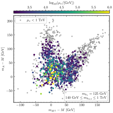
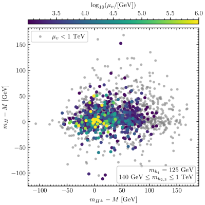
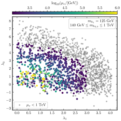
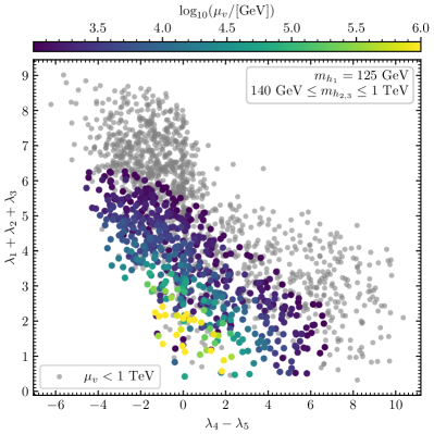
Figure 1: Top row: $m_{A}-M$ (left) and $m_{H}-M$ (right) in dependence of $m_{H^{\pm}}-M$, where $m_{H}=m_{h_{2}}$ or $m_{H}=m_{h_{2}}$ depending on whether $\Sigma_{h_{2}}<\Sigma_{h_{3}}$ or vice versa. Bottom row: $\lambda_{3}$ in dependence of $\lambda_{1}$ (left) and $\lambda_{1}+\lambda_{2}+\lambda_{3}$ in dependence of $\lambda_{4}-\lambda_{5}$ (right). The colour coding indicates the value of $\mu_{v}$. Also shown in grey are discarded parameter points with $\mu_{v}<1\ \mathrm{TeV}$.

In order to analyze the impact of the theoretical constraints, we show in Fig. 1 the parameter points with the colour coding indicating the energy scale $\mu_{v}$ until which the theoretical constraints are respected. We remind the reader that all parameter points fulfill the theoretical constraints at the initial scale $\mu=v$. All points for which $\mu_{v}<1\ \mathrm{TeV}$ are shown in grey. We performed the RGE running up to $\mu=100\ \mathrm{TeV}$, such that points that have $\mu_{v}=100\ \mathrm{TeV}$ (yellow points) are potentially valid up to much higher energy scales. In the upper left plot we show the parameter points in the plane $m_{H^{\pm}}-M$ and $m_{A}-M$. One can see that only points for which these differences are below roughly $50\ \mathrm{GeV}$ are valid at energy scales much beyond $1\ \mathrm{TeV}$. On the other hand, parameter points with values of $|m_{H^{\pm}}-M|\gtrsim 120\ \mathrm{GeV}$ and/or $|m_{A}-M|\gtrsim 150\ \mathrm{GeV}$ are always in contradiction with one of the theoretical constraints already at scales $\mu_{v}<1\ \mathrm{TeV}$. The same observation can be made in the upper right plot, in which $|m_{H}-M|$ is depicted on the vertical axis. Points that feature values of $\mu_{v}$ much larger than about $1\ \mathrm{TeV}$ are concentrated at values of $|m_{H}-M|\lesssim 50\ \mathrm{GeV}$, whereas points with larger values of $|m_{H}-M|$ are almost always only well behaved within a small range of energies.

We find that the relevant constraint that give rise to the low values of $\mu_{v}$ are in most cases the tree-level perturbative unitarity constraints. These constraints effectively provide upper limits on the absolute values of the quartic scalar couplings $\lambda_{i}$ and combinations thereof (see also App. B). It is therefore easy to understand why they are more severe in region of parameter space with relatively large splittings between the masses of the heavy BSM states and the mass scale $M$, since such splittings are induced by large absolute values of $\lambda_{1,2,3,4,5}$ (see also App. A). Moreover, for obvious reasons also the energy scale dependence of the quartic couplings is stronger when their absolute values are larger. As a result, points with large mass splittings, which potentially were already on the edge of being excluded via the tree-level perturbative unitarity constraints at the initial energy scale, quickly break one of these constraints once the RGE evolution is considered. This is also reflected in the plots in the lower row of Fig. 1, in which we show the points in the planes $\lambda_{1}$-$\lambda_{3}$ on the left and $(\lambda_{4}-\lambda_{5})$-$(\lambda_{1}+\lambda_{2}+\lambda_{3})$ on the right. In the left plot one can see that verifying the theoretical constraints exclusively at the initial scale $\mu=v$ gives rise to parameter points with values of $\lambda_{1}\lesssim 4$ and $-3\lesssim\lambda_{3}\lesssim 8$, whereas demanding that the constraints are respected within a range of energy of at least $v\leq\mu\leq 1\ \mathrm{TeV}$, the allowed ranges shrink to $\lambda_{1}\lesssim 3$ and $-2\lesssim\lambda_{3}\lesssim 5$. A similar observation can be made in the right plot, in which the allowed values change from $\lambda_{1}+\lambda_{2}+\lambda_{3}\lesssim 9$ and $-6\lesssim\lambda_{4}-\lambda_{5}\lesssim 10$ to $\lambda_{1}+\lambda_{2}+\lambda_{3}\lesssim 6$ and $-4\lesssim\lambda_{4}-\lambda_{5}\lesssim 7$ once the RGE running and the additional constraint $\mu_{v}>1\ \mathrm{TeV}$ is taken into account. Note that the limits on the values of the couplings that we found are much below the naive perturbativity criterion $|\lambda_{i}|<4\pi$, which is often applied in the analysis of extended Higgs sectors in order to exclude non-perturbative parameter regions.

Consequently, we conclude that regarding the collider phenomenology the main impact of our choice to demand the theoretical constraints to be respected at least until $\mu=1\ \mathrm{TeV}$ is that the masses of the heavy states are closely related to the overall mass scale $M$, which, however, does not significantly constrain the values of $\lambda_{6,7,8}$, since they do not depend directly on $M$ (see App. A). Thus, the only exception to the constraints on the mass splittings arises when there is a Higgs boson $h_{2}$ or $h_{3}$ with almost $100\%$ singlet component present, in which case its mass would be dominantly related to the value of $v_{S}$ instead of $M$, and the mass could differ substantially from $m_{A}$, $m_{H^{\pm}}$ and $m_{H}$, as will also be further discussed below. Thus, our approach of including the theoretical constraints drives the model predictions towards the decoupling limit of the S2HDM, where the masses of the heavy states $m_{A}$, $m_{H^{\pm}}$ and $m_{H}$ are approximately determined by the scale $M$ of the soft-breaking of the discrete $\mathbb{Z}_{2}$. Considering the theoretical constraints described above has in some aspects the same effect as applying the constraints from the EWPO, which are also sensitive to large mass splittings between the scalar states [106]. This fact on its own is not very surprising since also the EWPO observables arise from the radiative corrections. More interesting, however, is that while it is sufficient to have either $m_{H}\sim m_{H^{\pm}}$ or $m_{A}\sim m_{H^{\pm}}$ in order to be in agreement with the constraints from EWPO (at one-loop level), the inclusion of the RGE running and the requirement $\mu_{v}>1\ \mathrm{TeV}$ gives rise to the fact that both conditions should be approximately fulfilled, i.e. $m_{H}\sim m_{A}\sim m_{H^{\pm}}$.

The low values of $\mu_{v}$ that we found for values of $|\lambda_{i}|\gtrsim 1$ are relevant also for cosmological aspects of the S2HDM, where we stress again that one of the main motivations of the model is the possibility of accommodating a first-order EW phase transition. In order to achieve such a transition, it is required (just as in the 2HDM) to consider parameter space regions where large loop corrections to the scalar potential are present, since at tree level the scalar potential does not allow for an EW phase transition of first order. The required loop corrections have their origin in values of one or more ${|\lambda_{1,2,3,4,5}|>1}$ [33]. As a result, our analysis indicates that for a perturbative study of the parameter regions of the S2HDM relevant for possible first-order EW phase transitions, it is of crucial importance to take into account constraints in relation to the perturbative unitarity and the RGE running of the quartic couplings. On the other hand, if one restricts an analysis of the S2HDM to regions of the parameter space in which the couplings $\lambda_{i}$ have absolute values substantially below one, then the model can be valid to energy scales much beyond the TeV scale. In this case, however, the S2HDM cannot accommodate a first-order EW phase transition and its related phenomenology, and also the heavy BSM states are largely decoupled from the EW scale (as discussed above).

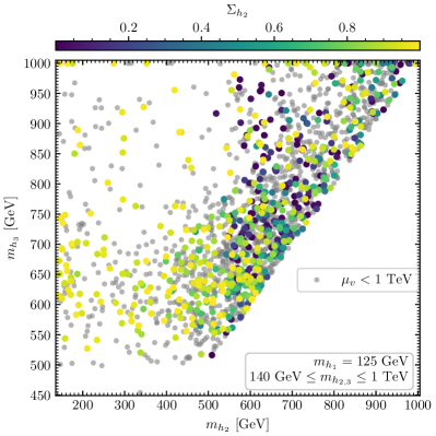
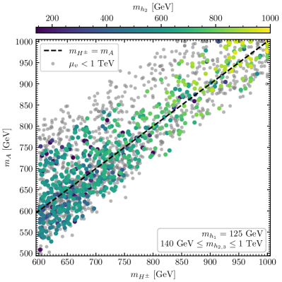
Figure 2: Spectrum of the heavy Higgs bosons $h_{2,3}$, $A$ and $H^{\pm}$ for the parameter points fulfilling the theoretical and experimental constraints. Left: $m_{h_{3}}$ in dependence of $m_{h_{2}}$, with the colours indicating $\Sigma_{h_{2}}$. Right: $m_{A}$ in dependence of $m_{H^{\pm}}$, with the colours indicating $m_{h_{2}}$. Also shown in grey are excluded parameter points with $\mu_{v}<1\ \mathrm{TeV}$. The dashed line indicates where $m_{H^{\pm}}=m_{A}$.

To shed more light on the spectrum of the Higgs bosons, we show in Fig. 2 the mass $m_{h_{3}}$ in dependence of $m_{h_{2}}$ on the left and $m_{A}$ in dependence on $m_{H^{\pm}}$ on the right. In the left plot one can see that it is possible that $h_{2}$ is substantially lighter than $h_{3}$ when it has a large singlet component of $\Sigma_{h_{2}}>90\%$, as indicated by the colours of the points. On the other hand, when $h_{2}$ and $h_{3}$ are sizably mixed, the masses of both states have to be relatively close to $M$ in order to comply with the theoretical constrains. The same observation can be made in the right plot regarding the masses of $A$ and $H^{\pm}$. Note here that all the points with $m_{A}-m_{H^{\pm}}\gtrsim 150\ \mathrm{GeV}$ are grey, indicating that they feature values of $\mu_{v}<1\ \mathrm{TeV}$. In this plot the colour coding indicates the values of $m_{h_{2}}$, and a correlation can be seen between the mass of $h_{2}$ and the masses of $A$ and $H^{\pm}$. The heavier the latter states, the larger also tend to be the values of $m_{h_{2}}$. Since by definition $m_{h_{2}}<m_{h_{3}}$, one can conclude that in most parameter points all six states $h_{2,3}$, $A$ and $H^{\pm}$ are relatively close in mass, with the only exception being a very singlet-like state $h_{2}$ with $m_{h_{2}}\ll M$, as mentioned earlier already. Hence, our analysis shows a trend towards the decoupling limit of the S2HDM, in which at low energies the model could become practically indistinguishable from the SM. In this case, the only possibility to observe a BSM effect would arise from the DM phenomenology or a possible invisible branching ratio of $h_{125}$ if the decay $h_{125}\to\chi\chi$ is kinematically allowed (see the discussion below). The presence of an invisible branching ratio of $h_{125}$ could also allow for a distinction between the S2HDM and the 2HDM, whereas the S2HDM in the decoupling limit could be practically indistinguishable from the pNG model with one Higgs doublet, in which case only a discovery of one of the additional particles of the S2HDM at a collider could shed light on the model realized in nature.

Going beyond the theoretical limitations, the spectrum of the Higgs bosons is also severely constrained by direct searches at colliders, where due to the fact that we focus here on the mass ordering with $h_{1}=h_{125}$ only the LHC results play a role in our discussion. Without going into the details of each of the relevant search channels, we list here the searches that were selected by HiggsBounds and which led to exclusions of parameter points in the scenario under investigation:

• ATLAS [122]: $gg\to A\to(h_{2})Z\to(b\bar{b})l^{+}l^{-}$ at $\sqrt{s}=13\ \mathrm{TeV}$

• ATLAS/CMS [123, 124]: $pp\to h_{2},h_{3}\to VV$ at $\sqrt{s}=13\ \mathrm{TeV}/7+8\ \mathrm{TeV}$

• ATLAS/CMS [125, 126]: $pp\to h_{2}\to ZZ$ at $\sqrt{s}=13\ \mathrm{TeV}$ and including width effects

• ATLAS [127]: $pp\to h_{2},h_{3},A\to\tau^{+}\tau^{-}$ at $\sqrt{s}=13\ \mathrm{TeV}$

• ATLAS [128]: $pp\to h_{2},h_{3}\to h_{1}h_{1}\to b\bar{b}b\bar{b}$ at $\sqrt{s}=13\ \mathrm{TeV}$

• CMS [129]: $gg\to A\to(h_{1})Z\to(b\bar{b})l^{+}l^{-}$ at $\sqrt{s}=13\ \mathrm{TeV}$ assuming $h_{1}=h_{125}$

• ATLAS [130]: $pp\to(H^{\pm})tb\to(tb)tb$ at $\sqrt{s}=13\ \mathrm{TeV}$

• ATLAS [131]: $pp\to h_{2},h_{3}\to h_{1}h_{1}$ at $\sqrt{s}=13\ \mathrm{TeV}$ assuming $h_{1}=h_{125}$

• CMS [132]: $gg\to h_{2},h_{3}\to t\bar{t}$ at $\sqrt{s}=13\ \mathrm{TeV}$ and including width effects

In general, the most promising searches at the lower end of the $\tan\beta$ range are the searches for the charged Higgs bosons or the searches for the neutral states $h_{2}$, $h_{3}$ and $A$ dominantly produced in the gluon fusion channel, where depending on their masses they then mostly decay into pairs of $t$ quarks, pairs of vector bosons or into a lighter Higgs boson and a $Z$ boson. For the upper end of the $\tan\beta$ range, the most promising channel is the resonant search for new Higgs bosons in the invariant mass spectrum of two $\tau$ leptons. Here it should be noted that the resulting exclusions in the S2HDM can be substantially different in comparison to the 2HDM, because $h_{3}$ and $A$ can have sizable branching ratios for the decays into final states containing a potentially much lighter singlet-like state $h_{2}$, in which case the branching ratios in regards to the decays of $h_{3}$ and $A$ into a pair of $\tau$-leptons are suppressed. As a result, for a fixed value of $\tan\beta$ both states can be lighter in the S2HDM compared to the 2HDM without being in conflict with the searches for heavy Higgs bosons decaying into two $\tau$ leptons [130]. Finally, for parameter points in the intermediate $\tan\beta$ range with $3\lesssim\tan\beta\lesssim 6$, the bosonic decays of the neutral states are most relevant, such that the searches with two vector bosons in the final state or Higgs cascade decays can probe parts of the parameter space of the S2HDM.

Complementary to the direct searches for the BSM particles, the Higgs sector of the S2HDM can also be probed indirectly via the properties of the Higgs boson $h_{1}=h_{125}$ resembling the Higgs boson that was discovered at the LHC. In order to illustrate the impact of such constraints, we show in the left plot of Fig. 3 the allowed parameter points, which all fulfill the criterion $\chi^{2}_{125}\leq\chi^{2}_{\mathrm{SM},125}+5.99$ (see Sect. 3.2 for details), with $\sin(\alpha-\beta)$ on the horizontal and $\tan\beta$ on the vertical axis. In the case in which one of the heavier states $h_{2}$ or $h_{3}$ has a singlet component of almost $100\%$, the S2HDM features an alignment limit similar to the 2HDM. In this limit the couplings of $h_{1}$ reduce to the ones of a SM Higgs boson, and the limit is determined by the condition $\sin(\alpha-\beta)=0$ (see also Ref. [76]). Consequently, departures from this condition are associated with deviations of the predictions for the signal rates of $h_{125}$ with respect to the SM. As can be seen in the left plot of Fig. 3, our analysis indicates that in order to be in agreement with the measured signal rates, one has to fulfill roughly $|\sin(\alpha-\beta)|\lesssim 0.1$. The largest departures from zero are found for the lower end of the $\tan\beta$ range, whereas for larger values of $\tan\beta$ the allowed range of $|\sin(\alpha-\beta)|$ shrinks substantially. The colour coding of the points indicates the singlet component of the SM-like Higgs boson $\Sigma_{h_{1}}$. Notably, we find that the current uncertainties of the signal-rate measurements still allow for a singlet-component of more than $14\%$.

Precise measurements of the properties of $h_{125}$, for instance correlated deviations from the SM prediction of the various different couplings coefficients of $h_{125}$ to the up- and down-type fermions $C_{h_{125}u\bar{u}}$ and $C_{h_{125}d\bar{d}}$ and the gauge bosons $C_{h_{125}VV}$, could help to distinguish the type II S2HDM from the usual 2HDM. Here the coupling coefficients $C_{h_{125}u\bar{u},d\bar{d},VV}$ are defined to be the couplings normalized to the ones of a SM Higgs boson. A sizable singlet-component of $h_{125}$, as found in parts of our parameter points, gives rise to a suppression of $C_{h_{125}VV}$. In the usual 2HDM, a deviation from $|C_{h_{125}VV}|\ =1$ is possible via departures from the alignment limit, and thus tightly constrained to values of $C_{h_{125}VV}^{2}\gtrsim 0.9$ [106]. Since we find parameter points with $\Sigma_{h_{125}}>0.1$, and since in the S2HDM one has $C_{h_{125}VV}^{2}\leq 1-\Sigma_{h_{125}}$, a possible future measurement indicating $C_{h_{125}VV}^{2}\lesssim 0.9$ at the (HL)-LHC would favor an S2HDM interpretation instead of the 2HDM. It is also interesting to compare the maximum values of $\Sigma_{h_{125}}\sim 14\%$ with the corresponding values found in the pNG DM model with only one Higgs doublet. In Ref. [23] it was shown that in this case the mixing of the SM-like Higgs boson with the singlet state is more constrained, and, except when the singlet scalar and the doublet scalar are degenerate in mass, only values of up to $10\%$ were found to be in agreement with the Higgs-boson measurements. As a result, and under the assumption that a deviation of the properties of $h_{125}$ w.r.t. the SM will be observed, one could potentially distinguish the S2HDM from the simpler model with only one Higgs doublet via the precise measurements of $C_{h_{125}VV}$, $C_{h_{125}u\bar{u}}$ and $C_{h_{125}d\bar{d}}$. Moreover, the model with one Higgs doublet predicts $C_{h_{125}u\bar{u}}=C_{h_{125}d\bar{d}}$, such that experimental indications for $C_{h_{125}u\bar{u}}\neq C_{h_{125}d\bar{d}}$ would clearly favour an S2HDM interpretation. Another obvious possibility to distinguish both models arises from the fact that the S2HDM can predict values of $|C_{h_{125}d\bar{d}}|,|C_{h_{125}u\bar{u}}|>1$ due to enhancements by factors of $1/c_{\beta}$ or $1/s_{\beta}$ (depending on the Yukawa type), while the pNG DM model with one Higgs doublet can only accommodate values equal or smaller than one.

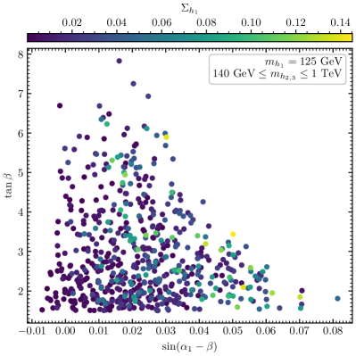
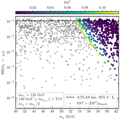
Figure 3: Left: $\tan\beta$ in dependence of $\sin(\alpha_{1}-\beta)$ for the parameter points that pass all the constraints discussed in Sect. 3. Right: Invisible branching ratio $\mathrm{BR}(h_{1}\to\chi\chi)$ in dependence of $m_{\chi}$ for the parameter points with $m_{\chi}<m_{h_{1}}/2$ that pass the constraints, not taking into account the experimental upper limit on $\mathrm{BR}(h_{1}\to\chi\chi)$ as reported by ATLAS [101]. The colour coding indicates $\Sigma_{h_{1}}$.

The mixing among the CP-even scalar fields in the S2HDM is identical to the one of the N2HDM, such that it is not surprising that we find similar effects on the allowed parameter ranges of $\alpha_{i}$ in the S2HDM. However, a crucial difference between both models is the presence of the additional particle $\chi$ in the S2HDM. Since we are focusing here on the Higgs funnel region of the model, it is possible that $m_{\chi}<125\ \mathrm{GeV}/2$, giving rise to an additional decay mode of $h_{125}$ into an invisible final state. To illustrate the impact of this additional decay on the allowed parameter regions, we show in the right plot of Fig. 3 the branching ratio for the invisible decay of $h_{125}$ in dependence of $m_{\chi}$ for the parameter points with $m_{\chi}<125\ \mathrm{GeV}/2$. Here we show also the parameter points that would be excluded by the observed upper limit on $\mathrm{BR}(h_{1}\to\chi\chi)$ [101] (indicated by the horizontal dashed line). In this way we can demonstrate the interplay between the global constraints from the HiggsSignals analysis and the direct limit on the invisible branching ratio. One can see that only a very small fraction of the otherwise allowed parameter points, which in particular have passed the constraint $\chi^{2}_{125}\leq\chi^{2}_{\mathrm{SM},125}+5.99$, lie above the ATLAS limit on the invisible branching ratio. Nevertheless, for some points we find values of $\mathrm{BR}(h_{1}\to\chi\chi)$ that are about $50\%$ larger than the upper limit in the whole range of $m_{\chi}$ in which allowed points were found.

The grey points in the right plot of Fig. 3 have to be discarded because they feature a too large thermal relic abundance of DM. For the allowed points the DM relic abundance is indicated by the colour coding of the points. One can see that we find a limit of $m_{\chi}\sim 53.8\ \mathrm{GeV}$ below which no allowed points were found. This limit arises from a combination of the upper limit on $\mathrm{BR}(h_{1}\to\chi\chi)$, on the one hand, and the constraint $\Omega h^{2}\leq(\Omega h^{2})_{\rm Planck}$, on the other hand. Parameter points with $m_{\chi}\lesssim 53.8\ \mathrm{GeV}$ feature either a $\chi$ that is weakly coupled to $h_{125}$, in which case $\mathrm{BR}_{\rm inv}$ can be in agreement with the ATLAS limit but the DM relic abundance is too large because the annihiliation process with $h_{125}$ in the $s$-channel is not efficient (see also discussion below), or $\chi$ is coupled more strongly to $h_{125}$, in which case the DM relic abundance can be below the upper limit but the invisible branching ratio of $h_{125}$ is unacceptably large. Note here that in the plot almost all parameter points with $m_{\chi}\lesssim 53.8\ \mathrm{GeV}$ belong to the first option, predicting too large values of $\Omega h^{2}$, while $\mathrm{BR}_{\rm inv}$ is below the experimental upper limit. On the other hand, there are only three parameter points with $m_{\chi}\lesssim 53.8\ \mathrm{GeV}$ belonging to the second option, featuring too large values of $\mathrm{BR}_{\rm inv}$ but with $\Omega h^{2}$ below the Planck limit. The reason for this lies in our procedure to generate the parameter points using the genetic algorithm. Parameter points with values of $\mathrm{BR}_{\rm inv}=\mathcal{O}(0.1)$ feature overall larger values of $\chi^{2}_{125}$ and constitute therefore only a very small part of the sample of parameter points, because the genetic algorithm tries to find parameter points that minimize $\chi^{2}_{125}$ (see the definition of the loss function defined in Eq. (9)).

The above discussed findings already indicate the strong interplay between the Higgs phenomenology and the DM sector of the S2HDM, in particular in the scenario discussed here that fundamentally relies on the Higgs funnel to predict a DM relic abundance in agreement with experiments. To shed more light on this interplay, we show in Fig. 4 the relic abundance as predicted according to the freeze-out mechanism in dependence of the DM mass $m_{\chi}$. One can see the strong suppression of $\Omega h^{2}$ for most parameter points at $m_{\chi}\sim 125/2\ \mathrm{GeV}$, where the DM annihilation cross sections with $h_{1}$ in the $s$-channel are resonantly enhanced. At this precise resonance region, there are nevertheless also a few parameter points featuring values of $\Omega h^{2}$ within an order of magnitude below the experimentally measured value $(\Omega h^{2})_{\rm Planck}=0.119$ (indicated by the grey dashed line in Fig. 4). For these parameter points the resonant enhancement of the annihilation cross sections is counteracted by strongly suppressed couplings of $\chi$ to $h_{125}$.

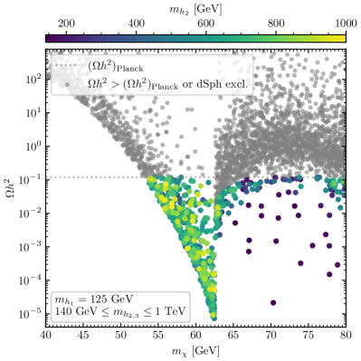
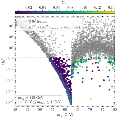
Figure 4: Relic abundance $\Omega h^{2}$ as predicted by thermal freeze-out in dependence of $m_{\chi}$. The colour coding indicates the values of $m_{h_{2}}$ (left) and the values of $\Sigma_{h_{2}}$ (right). Grey points are excluded by $\Omega h^{2}>(\Omega h^{2})_{\rm Planck}$ or Fermi dSph measurements.

For values of $m_{\chi}$ below $m_{h_{125}}/2$, there is a small band of values $53\ \mathrm{GeV}\lesssim m_{\chi}\lesssim m_{h_{125}}/2$ in which the measured value of the relic abundance can be accommodated, whereas for values below this range the predicted amount of DM density is always too large (grey points). As already mentioned before, the reason for this lies in the constraints on the properties of $h_{125}$. In order to predict an allowed value for $\Omega h^{2}$ when $m_{\chi}\lesssim 53\ \mathrm{GeV}$ it is required that the coupling of $\chi$ to $h_{125}$ is large. However, this inevitably results in values of the invisible branching ratio for the decay $h_{125}\to\chi\chi$ above the experimental upper limit. As a result, the lower limit on $m_{\chi}$ found here can be regarded as a robust bound under the assumption that $h_{125}$ corresponds to the lightest scalar $h_{1}$. One can compare also to the right plot of Fig. 4, where the colour coding indicates the values of the singlet component of the SM-like Higgs boson $h_{1}$. A clear distinction is visible between the points below and above the resonance at $m_{\chi}=125/2\ \mathrm{GeV}$. Points with $m_{\chi}$ below the resonance have substantially smaller values of $\Sigma_{h_{1}}$, whereas points with $m_{\chi}$ above the resonance allow for values of $\Sigma_{h_{1}}\gtrsim 0.1$. Moreover, only points for which $m_{\chi}$ is relatively close to the kinematic threshold of the decay $h_{1}\to\chi\chi$, i.e. $m_{\chi}\sim m_{h_{125}}/2$, feature sizable values of $\Sigma_{h_{1}}$ when $m_{\chi}<m_{h_{125}}/2$. The reason for this is that the couplings $\lambda_{7}$ and $\lambda_{8}$ that couple the singlet field to the doublet fields (see Eq. (2)) appear in the partial decay width for the invisible decay as shown in Eq. (6). In addition, these couplings are responsible for the possible singlet admixture of the state $h_{1}$. Accordingly, parameter points with sizable values of $\Sigma_{h_{1}}$ have sizable values of $\lambda_{7}$ and $\lambda_{8}$, which in turn can give rise to too large values of $\mathrm{BR}(h_{1}\to\chi\chi)$ whenever this decay is kinematically allowed. In Sect. 4.2 we will address the question whether the bound $m_{\chi}\gtrsim 53\ \mathrm{GeV}$ can be substantially modified in a scenario featuring a scalar $h_{1}$ with a mass smaller than $125\ \mathrm{GeV}$, and the second lightest scalar $h_{2}$ plays the role of the discovered Higgs boson. In this case $\chi$ has two possibilities to annihilate resonantly, either with $h_{1}$ or with $h_{2}$ in the $s$-channel, and the predictions for the relic abundance can be substantially modified.

For values of $m_{\chi}>125/2\ \mathrm{GeV}$ one can see that the prediction for $\Omega h^{2}$ rises quickly with increasing value of $m_{\chi}$, because the resonant enhancement of the annihilation cross section is lost. As a result, most parameter points predict a too large DM relic abundance. Taking into account the values of $m_{h_{2}}$ (indicated by the colour coding of the points in the left plot of Fig. 4), one can see that most parameter points with $m_{\chi}\gtrsim 65\ \mathrm{GeV}$ that are in agreement with the upper limit on $\Omega h^{2}$ feature a relatively light scalar $h_{2}$ with masses at the lower end of the scan range of $m_{h_{2}}$. As before, the reason for this is that when $h_{2}$ is not much heavier than twice the value of $m_{\chi}$, the second $s$-channel contribution to the annihilation cross section becomes relevant. This gives rise to a suppression of $\Omega h^{2}$ such that the prediction can be below the experimental limit even when $m_{\chi}$ is several GeV larger than $125/2\ \mathrm{GeV}$. Again, this hints to the fact that also in the mass range $m_{\chi}>125/2\ \mathrm{GeV}$ the prediction for $\Omega h^{2}$ could be substantially modified using the inverted mass hierarchy in which $h_{125}$ is not the lightest scalar, and we investigate this possibility assuming a Higgs boson $h_{1}$ at $96\ \mathrm{GeV}$ in Sect. 4.2.

In both plots in Fig. 4 the grey points are characterized by either being excluded due to $\Omega h^{2}>(\Omega h^{2})_{\rm Planck}$, as already mentioned before, or they are excluded due to the constraints from DM indirect-detection experiments. In most parts of the analyzed parameter space, the more constraining experimental limit results to be the upper limit on the predicted relic abundance, as indicated by the fact that most of the grey points lie above the horizontal dashed line indicating the Planck measurement. However, there is a small region with $62.5\ \mathrm{GeV}\lesssim m_{\chi}\lesssim 67\ \mathrm{GeV}$ in which we find grey points below the Planck limit. Consequently, in this mass range of $\chi$ the indirect-detection limits from the observation of dSph by the Fermi satellite are more constraining. Note that this is a region in which it appears to be relatively easy to accommodate a value of $\Omega h^{2}\sim(\Omega h^{2})_{\rm Planck}$ without being in tension with constraints on $h_{125}$, since it is just above the resonance of the annihilation cross section, and the decay $h_{125}\to\chi\chi$ is kinematically forbidden. The fact that these parameter points can be probed via indirect-detection experiments is therefore crucial. We remind the reader that the constraints derived from the Fermi measurements are subject to uncertainties, as was also discussed in Sect. 3.2, such that the respective limits might change slightly in the future and are currently possibly not as robust as the Planck limit on the relic abundance. Nevertheless, our results indicate that when the DM candidate of the S2HDM in this mass range is responsible for a large fraction of the measured relic abundance, the observation of dSph and the resulting constraints (or signals, more optimistically speaking) will be of great importance for studies in the context of pNG DM.

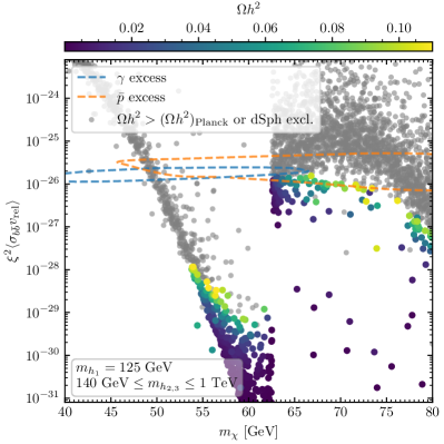
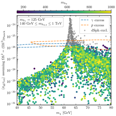
Figure 5: Today’s velocity averaged annihilation cross section of $\chi$ into pairs of $b$ quarks taking into account the number density as predicted by thermal freeze-out (left) and assuming $\Omega h^{2}=0.119$ (right). The colour coding indicates the predicted value of $\Omega h^{2}$ (left) and the value of $m_{h_{2}}$ (right). Also indicated are the regions in which the cosmic-rays excesses could be explained within the $2\sigma$ confidence level (blue and orange dashed lines) [66, 25]. Grey points are excluded by $\Omega h^{2}>(\Omega h^{2}_{\rm Planck})$ (left) or Fermi dSph measurements (left and right).

In this context it is interesting to note that recent indirect-detection experiments found anomalies in the cosmic ray spectra. The first so-called galactic center excess was found by the Fermi satellite, which measured an intensity of gamma-rays coming from the center of the galaxy significantly above the predictions of the standard model of cosmic rays generation and propagation with a peak in the spectrum around a few GeV [48, 49]. Another anomalous cosmic-ray spectra was measured by the Alpha Magnetic Spectrometer (AMS) [62], mounted on the international space station, which reported an excess over the expected flux of cosmic ray antiprotons (see Sect. 1 for details). While it is still under debate whether the excesses arise from unresolved astrophysical sources [59, 60, 61] or the treatment of systematic uncertainties [136, 137], or whether their origin could be the annihilation of DM, we will in the following assume that the latter is the case. In Ref. [66] it was shown that the excesses are compatible with a DM interpretation, where the DM candidate annihilates into pairs of $b$ quarks. For the $\gamma$ excess the allowed range of the mass of the DM candidate at the $2\sigma$ confidence level was found to be ${37\ \mathrm{GeV}\leq m_{\rm DM}\leq 67\ \mathrm{GeV}}$. For the $\bar{p}$ excess the allowed range was found to be ${46\ \mathrm{GeV}\leq m_{\rm DM}\leq 94\ \mathrm{GeV}}$, which partially agrees with the mass range preferred by the $\gamma$ excess. Consequently, it is an interesting question whether the S2HDM can explain both the excesses simultaneously, while being in agreement with all theoretical and experimental constraints.

In order to answer this question we show in Fig. 5 on the vertical axes $\langle\sigma_{b\bar{b}}v_{\rm rel}\rangle$, being the predicted velocity-averaged annihilation cross sections of $\chi$ into pairs of $b$ quarks, in dependence of the DM mass $m_{\chi}$ for the parameter points of our scan. The $2\sigma$ confidence level regions of these two parameters required to explain the $\gamma$ and the $\bar{p}$ excesses are indicated with the blue and orange dashed lines, respectively [66, 25]. We show the parameter points in the two plots of Fig. 5 under two different assumptions. In the left plot we assume that the usual thermal freeze-out scenario can be applied, such that we have to take into account the predicted values of the relic abundace for each parameter point. Hence, the values of $\langle\sigma_{b\bar{b}}v_{\rm rel}\rangle$ on the vertical axis are scaled by the factor $\xi^{2}$ as defined in Eq. (7). On the other hand, in the right plot we show the parameter points under the assumption that the relic abundance of DM is always accounted for by $\chi$, independently of the prediction from the thermal freeze-out. As a result, they demand a non-standard cosmological history giving rise to the experimentally measured relic abundance, which we will however not specify any further. In the plots the grey points correspond to parameter points that are excluded by a too large predicted relic abundance (left) or by constraints from dSph observations (left and right). In the right plot the dSph constraints are consequently applied also assuming $\Omega h^{2}=(\Omega h^{2})_{\rm Planck}$.

Assuming the usual thermal freeze-out scenario (left plot), one can see that the resonant structure of the distribution of the annihilation cross sections gives rise to two distinct regions of $m_{\chi}$ in which points inside the blue and the orange curves can be found. The first region at lower DM masses of $m_{\chi}\approx 50\ \mathrm{GeV}$ contains parameter points that predict values of $\xi^{2}\langle\sigma_{b\bar{b}}v_{\rm rel}\rangle$ as required for an explanation of the excesses, and where the values of $m_{\chi}$ lie roughly in the center of the values preferred by the $\gamma$ excesses and at the lower end of the range preferred by the $\bar{p}$ excess. However, these points are excluded because the predicted values of $\Omega h^{2}$ are about an order of magnitude larger than the experimentally measured value, as can also be seen in the left plot of Fig. 4. Accordingly, the parameter points in this region of $m_{\chi}$ are excluded and the cosmic-ray excesses cannot be realized there. The second region of DM masses in which points within both the blue and the orange curves are found is given by $63\ \mathrm{GeV}\lesssim m_{\chi}\lesssim 67\ \mathrm{GeV}$. However, as before, the corresponding points are shown in grey and are consequently excluded. Interestingly, here the responsible experimental constraint do not arise from the Planck measurement of the relic abundance, but from the Fermi-LAT observations of dSph, as was already discussed before. In fact, the predictions for $\Omega h^{2}$ in this range of $m_{\chi}$ are close or effectively identical to the Planck measurement. Hence, the points in this second region of DM masses possibly predict the correct DM relic abundance and could give rise to both the cosmic $\gamma$- and the $\bar{p}$-excesses, but they are in tension with the null-results from the observations of dSph. Here we remind the reader, as was discussed already in Sect. 3.2, that the Fermi-LAT dSph constraints are subject to uncertainties in regards to the astrophysical modelling of the spectral curves, and as a result might be slightly weaker as compared to applied here. Nevertheless, with future improvements of the dSph observations, for instance, due to the inclusion of more dSph and the increasing time periods of data taking, a firm exclusion (or confirmation if a DM signal will actually be found) of the parameter space region of the second DM mass range discussed here should be possible [143].

Under the assumption of a non-standard cosmological history that somehow gives rise to a relic abundance of $\chi$ in agreement with the Planck measurement (right plot), one can see that this time only one DM mass region with parameter points suitable for a realization of the excesses is present. Naturally, this region lies where the resonant enhancement of $\langle\sigma_{b\bar{b}}v_{\rm rel}\rangle$ is present, i.e. at $61\ \mathrm{GeV}\lesssim m_{\chi}\lesssim 67\ \mathrm{GeV}$, which consequently partially coincides with the second region of DM mass found in the left plot of Fig. 5. As before the points that lie within both the blue and the orange curves are in tension with the dSph observations from the Fermi satellite.

We end the discussion of the DM properties in this scan by noting that many of the above mentioned findings crucially depend on the assumed mass ordering of the CP-even Higgs bosons. In particular, the presence of a Higgs boson below $125\ \mathrm{GeV}$ can potentially impact the predictions for the relic abundance, as discussed in relation to Fig. 4. Moreover, the question whether the cosmic-ray excesses can be accommodated more easily when a second $s$-channel resonance for the annihilation cross section is available can be addressed. In Sect. 4.2 we will investigate these questions following the approach of Ref. [25], in which the presence of a Higgs boson at around $96\ \mathrm{GeV}$ was assumed in order to simultaneously explain also two collider excesses found at LEP in the $b\bar{b}$ final state and at the LHC in the diphoton final state.

pNG DM and a Higgs boson at $96\ \mathrm{GeV}$

In Ref. [25] it was used that the hypothetical particle state $h_{96}$ at $96\ \mathrm{GeV}$ can be coupled to new relatively light charged states that can give rise to additional contributions to the loop induced coupling of $h_{96}$ to photons in order to account for the diphoton excess found by CMS. In Ref. [69] it was shown that in the N2HDM the presence of the additional doublet Higgs field and the real singlet field are sufficient to accurately describe the collider excesses. Here, the diphoton rate was enhanced not via an enhancement of the coupling coefficient $|C_{h_{96}\gamma\gamma}|$, where the coupling coefficients $C_{h_{96}\dots}$ are defined as the coupplings normalized to the one of a SM Higgs boson of the same mass. Instead, the branching ratio for the diphoton decay of $h_{96}$ was enhanced via a suppression of the couplings of $h_{96}$ to $b$ quarks, which then also gives rise to a suppression of the total width of $h_{96}$. The required suppression of the coupling coefficient $|C_{h_{96}b\bar{b}}|$ (without suppressing $|C_{h_{96}t\bar{t}}|$ in order to maintain sizable couplings to photons via the $t$-quark loop) can also be realized in the S2HDM due to the possible mixing patterns in the CP-even sector and the presence of the three mixing angles $\alpha_{1,2,3}$ in total analogy to the N2HDM. In this regard, the only difference in the S2HDM compared to the N2HDM is the possible presence of the additional decay modes $h_{96}/h_{125}\to\chi\chi$, potentially giving rise to a small suppression of the decay modes $h_{96}\to\gamma\gamma$ relevant for the CMS excess and $h_{96}\to b\bar{b}$ relevant for the LEP excess, or to stronger constrains on the properties of $h_{125}$. In the following we will discuss a scan to illustrate the impact of the presence of $h_{96}$ on the phenomenology of the DM candidate $\chi$, and whether the collider excesses can be realized in combination with the cosmic-ray excesses.

Before going into the description of the parameter scan that we performed, we briefly introduce the relevant details of the collider excesses. At LEP searches for Higgs bosons were performed utilizing the $b\bar{b}$ final state [144], which can be exploited at a lepton collider in contrast to the LHC due to the much smaller SM background. Theoretically, the Higgs boson that is searched for is assumed to be produced via the Higgstrahlung pocess and subsequently decays into a pair of $b$ quarks. A local excess of about $2\sigma$ confidence level was observed at a mass of roughly $96\ \mathrm{GeV}$, where the mass resolution is rather poor due to the hadronic final state. In Ref. [70] it was shown that the excess is consistent with a signal interpretation corresponding to a signal strength of

$$\mu_{\rm LEP}^{\rm exp}=0.117\pm 0.057\ .$$ (10)

Low-mass Higgs-boson searches have also been performed at the LHC in various final states. CMS searched for light Higgs bosons in the diphoton final state utilizing the $8\ \mathrm{TeV}$ and parts of the $13\ \mathrm{TeV}$ datasets [145]. A local excess of roughly $3\sigma$ confidence level was observed at a mass of $96\ \mathrm{GeV}$, hence in agreement with the mass range compatible with the LEP excess. In this case the excess is consistent with a signal interpretation corresponding to a signal strength of

$$\mu_{\rm CMS}^{\rm exp}=0.6\pm 0.2\ .$$ (11)

In our scan, in which $h_{1}$ will play the role of the state $h_{96}$, we compare the theoretical predictions for the signal strengths to the experimental values given above. The predictions were calculated by

$$\mu_{\rm LEP}\approx\frac{C_{h_{96}VV}^{2}\cdot\mathrm{BR}\left(h_{96}\to b\bar{b}\right)}{\mathrm{BR}^{\rm SM}\left(H\to b\bar{b}\right)}\ ,\quad\mu_{\rm CMS}\approx\frac{C_{h_{96}t\bar{t}}^{2}\cdot\mathrm{BR}\left(h_{96}\to\gamma\gamma\right)}{\mathrm{BR}^{\rm SM}\left(H\to\gamma\gamma\right)}\ .$$ (12)

Hence, in both cases the cross section ratios that enter the definitions of the signal strengths are expressed to a very good approximation in terms of the effective coupling coefficients ${C_{h_{96}VV}=c_{\alpha_{2}}c_{\beta-\alpha_{1}}}$ and ${C_{h_{96}t\bar{t}}=s_{\alpha_{1}}c_{\alpha_{2}}/s_{\beta}}$, which, as mentioned already, are defined as the couplings of $h_{96}$ normalized to the respective couplings of a SM Higgs boson with the same mass. The values for the SM branching ratios in the denominator, again assuming a SM Higgs boson at $96\ \mathrm{GeV}$, can be found in the literature [146]. From the theoretical predicted values $\mu_{\rm LEP,CMS}$ and the experimentally determined values $\mu_{\rm LEP,CMS}^{\rm exp}$ and their uncertainties we construct a $\chi^{2}$ function

$$\chi^{2}_{96}=\frac{\left(\mu_{\rm LEP}-0.117\right)^{2}}{0.057^{2}}+\frac{\left(\mu_{\rm CMS}-0.6\right)^{2}}{0.2^{2}}\ ,$$ (13)

in order to quantify the goodness of the fits to the excesses. In this definition we assumed that there is no correlation between both measurements.

Technically, the details of the scan that we discuss here are very similar to the ones of the scan discussed in Sect. 4.1. The scan ranges were set as given in Eq. (8), except for the masses of the scalars, which were chosen to be

$$m_{h_{1}}=96\ \mathrm{GeV}\ ,\quad m_{h_{2}}=125.09\ \mathrm{GeV}\ ,\quad m_{h_{3}}=m_{H}\leq 1\ \mathrm{TeV}\ ,$$ (14)

such that $m_{h_{3}}=m_{H}$ is further constrained by the condition $\Delta M_{\rm max}<200\ \mathrm{GeV}$, as defined in Eq. (8) and substantially heavier than $h_{1}$ and $h_{2}$ due to the lower limit on $m_{H^{\pm}}$. We again followed the two-step procedure. In the first step, we used the genetic algorithm to obtain parameter points in agreement with the theoretical constraints and the experimental constraints from the Higgs phenomenology. To the loss function defined in Eq. (9) we added a term $10\chi^{2}_{96}$ in order to obtain parameter points that potentially feature both a good fit to the signal rates of the SM-like Higgs boson $h_{2}=h_{125}$ and to the signal rates $\mu_{\rm LEP}$ and $\mu_{\rm CMS}$. All parameter points obtained by the help of the genetic algorithm were subject to the constraint

$$\chi^{2}_{125}+\chi^{2}_{96}\leq\chi^{2}_{\mathrm{SM},125}+\chi^{2}_{\mathrm{SM},96}\ ,\quad\chi^{2}_{\mathrm{SM},125}=84.41\ ,\quad\chi^{2}_{\mathrm{SM},96}=13.99\ ,$$ (15)

where the value of $\chi^{2}_{\mathrm{SM},96}$ is obtained from Eq. (13) assuming zero values for both $\mu_{\rm LEP}$ and $\mu_{\rm CMS}$ as predicted by the SM, in which no particle is present at a mass of $96\ \mathrm{GeV}$. As a result, in comparison to the analysis discussed in Sect. 4.1 in which the requirement $\chi^{2}_{125}\leq\chi^{2}_{\mathrm{SM},125}$ was used, the requirement shown in Eq. (15) allows for larger values of $\chi^{2}_{125}$ as long as the S2HDM parameter point provides a good fit to the collider excesses, i.e. it features values of $\chi^{2}_{96}\ll\chi^{2}_{\mathrm{SM},96}$. Here it should be noted that even in the most extreme case with $\chi^{2}_{96}=0$ the allowed maximum value of $\chi^{2}_{125}$ still does not indicate severe modifications of the signal rates of $h_{125}$, taking into account that the HiggsSignals fit result applies a total amount of 107 observables, such that the reduced $\chi^{2}$ value remains substantially smaller than one even in this case. The second step is totally analogue to the scan discussed in Sect. 4.1. All parameter points that pass the constraint shown in Eq. (15) were confronted with the theoretical constraints including now the RGE evolution of the parameters. As before, we required the scalar potential to be well behaved up to energy scale of at least $\mu_{v}=1\ \mathrm{TeV}$, such that in particular the values of the quartic couplings $\lambda_{i}$ allow for a perturbative treatment at the range of energy at which there are also particle masses in our scan. Finally, the remaining experimental constraints regarding the DM phenomenology were applied.

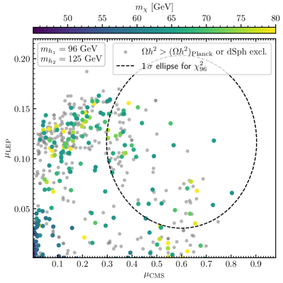
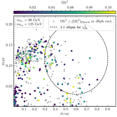
Figure 6: $\mu_{\rm LEP}$ in dependence of $\mu_{\rm CMS}$, with the colour coding indicating the values of $m_{\chi}$ (left) and $\Omega h^{2}$ (right). Grey points are excluded by $\Omega h^{2}>(\Omega h^{2})_{\rm Planck}$ or Fermi dSph measurements. The dashed ellipse indicates the experimentally preferred region of the collider excesses at the $1\sigma$ confidence level.

We show the resulting parameter points in Fig. 6, where we display the signal rate $\mu_{\rm LEP}$ in dependence of $\mu_{\rm CMS}$. We indicate with the colour coding of the points the value of the DM mass $m_{\chi}$ (left) and the DM relic abundance $\Omega h^{2}$ as predicted by the usual thermal freeze-out scenario (right). Also shown as grey points are parameter points that are excluded by a too large prediction of the relic abundance or by limits coming from observations of dSph. The ellipse in both plots indicates the region in agreement with the collider excesses at the $1\sigma$ confidence level, i.e. $\chi^{2}_{96}=2.3$. One can see that we find parameter points within the ellipses. Consequently, both excesses can be explained simultaneously while taking into account the constraints described in Sect. 3. In the left plot, we observe that parameter points with sizable values of $\mu_{\rm LEP}$ and $\mu_{\rm CMS}$ feature DM mass values close to or larger than $m_{h_{125}}/2$. On the other hand, parameter points with $m_{\chi}<m_{h_{125}}/2$ only predict substantially smaller signal strengths, and the collider excesses cannot be accounted for. The reason for this is, as was also discussed in Sect. 4.1, that in this case the decay $h_{125}\to\chi\chi$ is kinematically open. As a result, the possible mixing of the singlet field $h_{1}=h_{96}$ with the SM-like Higgs boson $h_{2}=h_{125}$ is much more constrained. However, a sizable mixing of $h_{96}$ and $h_{125}$ is necessary to obtain values of $\mu_{\rm LEP}$ and $\mu_{\rm CMS}$ of the order of the experimentally measured values. We therefore can conclude that a realization of the collider excesses demands DM masses of $m_{\chi}>m_{h_{125}}/2$. In the right plot of Fig. 6 we find that several of the parameter points that are able to explain both excesses also predict sizable values for the relic abundance, with some parameter points saturating the value measured by the Planck collaboration. Accordingly, we come to the conclusion that the S2HDM can accommodate the collider excesses at $96\ \mathrm{GeV}$ while at the same time accommodating a large fraction or all of the measured DM relic abundance.

In Fig. 7 the predicted relic abundance is shown in dependence of the DM mass. The values of the signal rates measured by LEP (left) and CMS (right) are also indicated by the colour coding of the points. We note a new prominent feature in the distribution of the parameter points with respect to Fig. 4. Due to the opening of a new resonant $s$-channel mediated by the $h_{96}$, parameter points featuring DM masses smaller than about $53\ \mathrm{GeV}$ can now be in agreement with the upper limit imposed by the observed DM relic abundance. Moreover, the presence of $h_{96}$ also gives rise to the fact that a large fraction of parameter points with $m_{\chi}>m_{h_{125}}/2$ lie below the Planck limit, whereas we found in Sect. 4.1 (compare to Fig. 4) that in this DM mass region most points predict $\Omega h^{2}>(\Omega h^{2})_{\rm Planck}$. Grey points that lay below the experimental upper limit are excluded by dSph observations. Here it is interesting to note that we find, in addition to the region around $m_{\chi}\sim 63\ \mathrm{GeV}$ already present in Fig. 4, a second region at $48\ \mathrm{GeV}\lesssim m_{\chi}\lesssim 58\ \mathrm{GeV}$ in which the dSph constraints discard points that would be in agreement with the Planck measurement of the DM relic abundance. In the left plot of Fig. 7 we find that for the points at the right side of the resonance the predicted values of $\mu_{\rm LEP}$ can be close to the measured central value $\mu_{\rm LEP}^{\rm exp}=0.117$ independently of the precise value of $m_{\chi}$. On the contrary, as can be seen in the right plot of Fig. 7, values of $\mu_{\rm CMS}\sim\mu_{\rm CMS}^{\rm exp}=0.6$ that are in agreement with the constraints are mostly found in the interval $62\ \mathrm{GeV}\lesssim m_{\chi}\lesssim 65\ \mathrm{GeV}$. For larger values of $m_{\chi}$ one can still find parameter points that fit the CMS excess at the level of $1\sigma$. However, they often predict too large values of $\Omega h^{2}>(\Omega h^{2})_{\rm Planck}$ and are therefore shown mostly as grey points. The reason for this is that, as discussed before, fitting the diphoton excess requires a suppression of the couplings of $h_{96}$ to $b$ quarks. However, this then yields also a suppression of the annihilation cross section via the process $\chi\chi\to h_{96}\to b\bar{b}$.

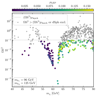
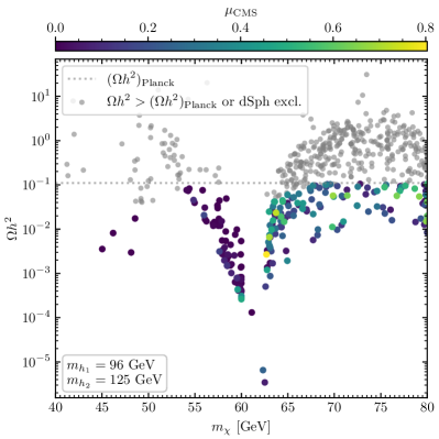
Figure 7: $\Omega h^{2}$ in dependence of $m_{\chi}$, with the colour coding indicating the values of $\mu_{\rm LEP}$ (left) and $\mu_{\rm CMS}$ (right). Grey points are excluded by $\Omega h^{2}>(\Omega h^{2})_{\rm Planck}$ or Fermi dSph measurements.

In order to discuss the gamma-ray and the antiproton excesses, we show in Fig. 8 today’s velocity-averaged annihilation cross section of $\chi$ into pairs of $b$ quarks taking into account the number density as predicted by thermal freeze-out (left) and assuming $\Omega h^{2}=0.12$ (right), as explained in Sect. 4.1. In comparison to Fig. 5, here we observe that there are more regions of $m_{\chi}$ in which points are found inside the preferred region to explain both cosmic-ray excesses simultaneously. These points remain in tension with present limits imposed by the observation of dSph. We remind the reader about the uncertainties in determining those limits (see Sect. 3.2 for more details). Regarding the agreement with the signal rate $\mu_{\rm CMS}$, only the parameter points situated towards the right end of the blue curve could simultaneously explain the two cosmic ray and the CMS excesses. These points are again in tension with indirect-detection limits from dSph observations. Regardless of whether the collider excesses are accommodated or not, we see that the presence of $h_{96}$ gives rise to more points at the lower end of $m_{\chi}$ that lie within the blue and the orange curves. Thus, the new light scalar state gives rise to new interesting regions of parameter space with $m_{\chi}<60\ \mathrm{GeV}$ in the context of the cosmic-ray anomalies. However, as was already mentioned, the collider excesses, which were the main motivation to investigate a scenario with $m_{h_{1}}=96\ \mathrm{GeV}$ in the first place, cannot be realized here.

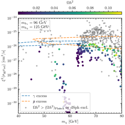
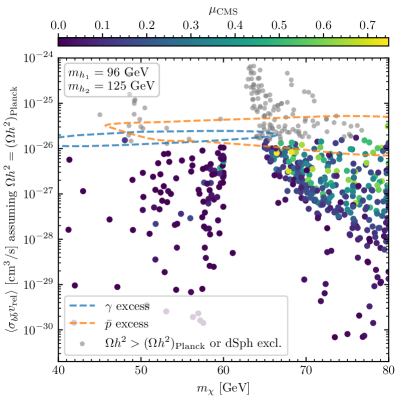
Figure 8: Today’s velocity averaged annihilation cross section of $\chi$ into pairs of $b$ quarks taking into account the number density as predicted by thermal freeze-out (left) and assuming $\Omega h^{2}=0.119$ (right). The colour coding indicates the predicted value of $\Omega h^{2}$ (left) and the value of $m_{h_{2}}$ (right). Also indicated are the regions in which the cosmic-rays excesses could be explained (blue and orange dashed lines) [54, 66]. Grey points are excluded by $\Omega h^{2}>(\Omega h^{2}_{\rm Planck})$ (left) or Fermi dSph measurements (left and right).

5 Conclusions

In this paper we analyzed a singlet-extended 2HDM, called S2HDM, which is a model with a rich Higgs phenomenology and that incorporates a pseudo-Nambu-Goldstone boson dark matter candidate. We focused on the parameter space of the S2HDM featuring DM masses in the Higgs funnel region, i.e. $40\ \mathrm{GeV}\leq m_{\chi}\leq 80\ \mathrm{GeV}$. One of the main purposes of this analysis was to illustrate the combined impact of various theoretical and experimental constraints on the model parameters, where in particular the strong interplay between the Higgs-sector phenomenology and the DM sector of the S2HDM was demonstrated. We required the scalar potential to be well-behaved up to energy scales of $1\ \mathrm{TeV}$, i.e. to be bounded-from-below, to feature a stable electroweak vacuum and to fulfill conditions derived from perturbative unitarity. We also ensured that the parameter points were in agreement with measurements of electroweak precision observables, flavour physics, properties of the discovered Higgs boson at $125\ \mathrm{GeV}$, searches for additional scalar states, and the DM observables. The model exploration of the multi-dimensional parameter space of the S2HDM was performed with the help of a genetic algorithm, by which, compared to random scans of the parameters, a significant improvement of the computing time required to find viable parameter points was achieved.

In our numerical analysis, we focused on two benchmark scenarios. Firstly, we performed a broad parameter scan assuming that the SM-like Higgs boson $h_{125}$ was the lightest of the three CP-even Higgs bosons, such that the predictions for the DM relic abundance assuming the usual thermal freeze-out mechanism are mainly determined by the resonant $s$-channel annihilation mediated by $h_{125}$. Secondly, we studied a scenario featuring a singlet-like CP-even state $h_{96}$ at $96\ \mathrm{GeV}$, where the presence of $h_{96}$ also gives rise to a second $s$-channel contribution to the thermal freeze-out cross section and today’s annihilation cross section relevant for DM indirect-detection experiments.

In the first scenario in which $h_{125}$ is assumed to be the lightest CP-even scalar, DM masses $62.5\ \mathrm{GeV}\lesssim m_{\chi}\lesssim 67\ \mathrm{GeV}$ were found to be able to explain the $\gamma$-ray and antiproton cosmic rays excesses, while simultaneously also predicting values of the DM relic abundance in agreement with the observations by the Planck collaboration. However, these parameter points are in tension with indirect-detection limits derived from observations of dwarf spheroidal galaxies, where it should be taken into account that these constraints are still subject to uncertainties with regards to the astrophysical modelling of the spectral curves. Concerning the Higgs phenomenology, we found that demanding that the theory can be treated perturbatively up to energy scales of at least $1\ \mathrm{TeV}$ has a strong impact on the Higgs spectra that can be realized. Namely, the mass splittings among the heavy scalar states $H^{\pm}$, $A$ and $h_{2,3}$ were found to be smaller than roughly $100\ \mathrm{GeV}$, driving the model towards the decoupling limit, with the only exception of a very singlet-like CP-even state $h_{i}$, which can be substantially lighter (or heavier) than the other BSM state without giving rise to issues with unperturbative effects at energy scales below $1\ \mathrm{TeV}$.

In the second scenario, we studied whether the S2HDM could offer an explanation for the collider excesses observed at about $96\ \mathrm{GeV}$ at LEP and CMS in the $b\bar{b}$ and the diphoton final state, respectively. Here we found that a singlet-like CP-even Higgs boson at $96\ \mathrm{GeV}$ can reproduce both collider excesses under the constraint that $m_{\chi}>m_{h_{125}}/2$ in order to allow for a sizable mixing between $h_{96}$ and $h_{125}$. Furthermore, it is possible to accommodate at the same time a large fraction or all of the measured DM relic abundance. Finally, we found that the simultaneous explanation of the cosmic-ray excesses and the collider excess at $96\ \mathrm{GeV}$ is in principle possible, but, as in the first scenario, the parameter points are also in tension with limits arising from observations of dwarf spheroidal galaxies.

To summarize, we demonstrated that the S2HDM is an attractive model that can accommodate a rich phenomenology and an interesting interplay between the DM sector and the Higgs sector. We also showed that it is crucial to take into account the various theoretical and experimental constraints on the model parameters. For future studies, we make our implementation of the model predictions and the application of the constraints available to the public in the form of a python package called s2hdmTools, which is briefly described in App. C.

Appendix A Parameter transformations

In the following we give the transformation formulae between the basis of the Lagrangian parameters and the physical basis chosen to scan the parameter space of the S2HDM defined in Eq. (5). The quartic couplings $\lambda_{i}$ can be written in terms of the physical basis as

$$\lambda_{1} =\frac{1}{v^{2}c_{\beta}^{2}}\left(-M^{2}s_{\beta}^{2}+\sum_{n=1}^{3}m_{h_{i}}^{2}R_{i1}^{2}\right)\ ,$$ (16)

$$\lambda_{2} =\frac{1}{v^{2}s_{\beta}^{2}}\left(-M^{2}c_{\beta}^{2}+\sum_{n=1}^{3}m_{h_{i}}^{2}R_{i2}^{2}\right)\ ,$$ (17)

$$\lambda_{3} =\frac{1}{v^{2}}\left(-M^{2}+\frac{1}{c_{\beta}s_{\beta}}\left(\sum_{n=1}^{3}m_{h_{i}}^{2}R_{i1}^{2}R_{i2}^{2}\right)+2m_{H^{\pm}}^{2}\right)\ ,$$ (18)

$$\lambda_{4} =\frac{1}{v^{2}}\left(M^{2}+m_{A}^{2}-2m_{H^{\pm}}^{2}\right)\ ,$$ (19)

$$\lambda_{5} =\frac{1}{v^{2}}\left(M^{2}-m_{A}^{2}\right)\ ,$$ (20)

$$\lambda_{6} =\frac{1}{v_{S}^{2}}\left(\sum_{n=1}^{3}m_{h_{i}}^{2}R_{i3}^{2}\right)\ ,$$ (21)

$$\lambda_{7} =\frac{1}{vv_{S}c_{\beta}}\left(\sum_{n=1}^{3}m_{h_{i}}^{2}R_{i1}R_{i3}\right)\ ,$$ (22)

$$\lambda_{8} =\frac{1}{vv_{S}s_{\beta}}\left(\sum_{n=1}^{3}m_{h_{i}}^{2}R_{i2}R_{i3}\right)\ ,$$ (23)

where the matrix elements $R_{ij}$ have been defined in terms of the mixing angles $\alpha_{1,2,3}$ in Eq. (4). With the previous transformations, one can also compute the mass parameters in the scalar potential using the tadpole equations as follows,

$$\mu_{11}^{2} =m_{12}^{2}\tan\beta-\frac{1}{2}\left(\lambda_{1}v^{2}c_{\beta}^{2}+(\lambda_{3}+\lambda_{4}+\lambda_{5})v^{2}s_{\beta}^{2}+\lambda_{7}v_{S}^{2}\right)\ ,$$ (24)

$$\mu_{22}^{2} =\frac{m_{12}^{2}}{\tan\beta}-\frac{1}{2}\left(\lambda_{2}v^{2}s_{\beta}^{2}+(\lambda_{3}+\lambda_{4}+\lambda_{5})v^{2}c_{\beta}^{2}+\lambda_{8}v_{S}^{2}\right)\ ,$$ (25)

$$\mu_{\chi}^{2} =m_{\chi}^{2}\ ,$$ (26)

$$\mu_{S}^{2} =m_{\chi}^{2}-\left(\lambda_{7}v^{2}c_{\beta}^{2}+\lambda_{8}v^{2}s_{\beta}^{2}+\lambda_{6}v_{S}^{2}\right)\ .$$ (27)

Appendix B Tree-level perturbative unitarity constraints

Here we list the tree-level perturbative unitarity conditions that were applied in our analysis in order to exclude parameter points which cannot be treated perturbatively:

$$\left|\lambda_{3}+\lambda_{4}\right| \leq 8\pi$$ (28)

$$\frac{1}{2}\left|\lambda_{1}+\lambda_{2}-\sqrt{\lambda_{1}^{2}-2\lambda_{2}\lambda_{1}+\lambda_{2}^{2}+4\lambda_{4}^{2}}\right| \leq 8\pi$$ (29)

$$\frac{1}{2}\left|\lambda_{1}+\lambda_{2}+\sqrt{\lambda_{1}^{2}-2\lambda_{2}\lambda_{1}+\lambda_{2}^{2}+4\lambda_{4}^{2}}\right| \leq 8\pi$$ (30)

$$\left|\lambda_{3}+2\lambda_{4}-3\lambda_{5}\right| \leq 8\pi$$ (31)

$$\left|\lambda_{3}-\lambda_{5}\right| \leq 8\pi$$ (32)

$$\left|\lambda_{3}+\lambda_{5}\right| \leq 8\pi$$ (33)

$$\left|\lambda_{3}+2\lambda_{4}+3\lambda_{5}\right| \leq 8\pi$$ (34)

$$\frac{1}{2}\left|\lambda_{1}+\lambda_{2}-\sqrt{\lambda_{1}^{2}-2\lambda_{2}\lambda_{1}+\lambda_{2}^{2}+4\lambda_{5}^{2}}\right| \leq 8\pi$$ (35)

$$\frac{1}{2}\left|\lambda_{1}+\lambda_{2}+\sqrt{\lambda_{1}^{2}-2\lambda_{2}\lambda_{1}+\lambda_{2}^{2}+4\lambda_{5}^{2}}\right| \leq 8\pi$$ (36)

$$\left|\lambda_{6}\right| \leq 8\pi$$ (37)

$$\left|\lambda_{7}\right| \leq 8\pi$$ (38)

$$\left|\lambda_{8}\right| \leq 8\pi$$ (39)

$$\left|\lambda_{3}-\lambda_{4}\right| \leq 8\pi$$ (40)

$$\frac{1}{2}\Bigg{|}\text{Roots}\Big{[}x^{3}+\left(-6\lambda_{1}-6\lambda_{2}-4\lambda_{6}\right)x^{2}+\big{(}-16\lambda_{3}^{2}-16\lambda_{4}\lambda_{3}-4\lambda_{4}^{2}- 8\lambda_{7}^{2}-8\lambda_{8}^{2}+$$

$$36\lambda_{1}\lambda_{2}+24\lambda_{1}\lambda_{6}+24\lambda_{2}\lambda_{6}\big{)}x+48\lambda_{2}\lambda_{7}^{2}+48\lambda_{1}\lambda_{8}^{2}+64\lambda_{3}^{2}\lambda_{6} +16\lambda_{4}^{2}\lambda_{6}-$$

$$144\lambda_{1}\lambda_{2}\lambda_{6}+64\lambda_{3}\lambda_{4}\lambda_{6}-64\lambda_{3}\lambda_{7}\lambda_{8}- 32\lambda_{4}\lambda_{7}\lambda_{8},x\Big{]}\Bigg{|}\leq 8\pi$$ (41)

Appendix C The python package s2hdmTools

In order to make the analysis of the S2HDM as performed here publicly available, we developed the python package s2hdmTools. The code can be downloaded at https://gitlab.com/thomas.biekoetter/s2hdmtools. The installation requires a python3 environment and compilers for Fortran, C and C++. In addition, a python2 installation is required for the external code MadDM. During the installation process, the following external codes are downloaded and installed:

• AnyHdecay [97, 98, 99, 76, 100]: Calculates partial decay widths of the Higgs bosons

• HiggsBounds [87, 88, 89, 90, 91, 92]: Tests against constraints from Higgs-boson searches at colliders

• HiggsSignals [93, 94, 95, 96]: Test against constraints from measurements of $h_{125}$

• Hom4PS2 [79]: Solver of system of polynomial equations

• MicrOmegas [113]: Calculation of relic abundance of dark matter

• MadGraph [117]: Monte-Carlo event generator

• MadDM [115, 116]: Test against constraints from indirect-detecion experiments for dark matter

The user interface of s2hdmTools is defined in the class ParamPoint and briefly summarized in the README. The most important features can be accessed via the following functions defined in ParamPoint:

• pt = ParamPoint(dc): Initializes a parameter point given a dictionary dc containing the values of the input parameters

• pt.check_theory_constraints(): Verifies whether the theoretical constraints are fulfilled, optionally up to an energy scale as provided by the user

• hbhs.check_point(pt): Applies the HiggsBounds- and HiggsSignals test

• pt.check_ewpo(): Checks against constraints from electroweak precision observables

• pt.check_darkmatter(): Computes dark matter observables and checks against constraints on the relic abundance and on today’s annihilation cross sections from dSph observations

More instructions regarding the installation and the usage of the package can be found in the documentation under the link:

https://www.desy.de/~biek/s2hdmtoolsdocu/site/

In addition, the application folder of the git repository contains some of the scripts that were used in order to produce the results discussed here.

References

- [1] ATLAS collaboration, Observation of a new particle in the search for the Standard Model Higgs boson with the ATLAS detector at the LHC, Phys. Lett. B 716 (2012) 1 [1207.7214].
- [2] CMS collaboration, Observation of a New Boson at a Mass of 125 GeV with the CMS Experiment at the LHC, Phys. Lett. B 716 (2012) 30 [1207.7235].
- [3] ATLAS, CMS collaboration, Measurements of the Higgs boson production and decay rates and constraints on its couplings from a combined ATLAS and CMS analysis of the LHC pp collision data at and 8 TeV, JHEP 08 (2016) 045 [1606.02266].
- [4] ATLAS collaboration, Combined measurements of Higgs boson production and decay using up to fb-1 of proton-proton collision data at 13 TeV collected with the ATLAS experiment, Phys. Rev. D 101 (2020) 012002 [1909.02845].
- [5] CMS collaboration, Combined measurements of Higgs boson couplings in proton–proton collisions at , Eur. Phys. J. C 79 (2019) 421 [1809.10733].
- [6] F. Zwicky, Die Rotverschiebung von extragalaktischen Nebeln, Helv. Phys. Acta 6 (1933) 110.
- [7] V.C. Rubin and W.K. Ford, Jr., Rotation of the Andromeda Nebula from a Spectroscopic Survey of Emission Regions, Astrophys. J. 159 (1970) 379.
- [8] R. Massey, T. Kitching and J. Richard, The dark matter of gravitational lensing, Rept. Prog. Phys. 73 (2010) 086901 [1001.1739].
- [9] D. Clowe, M. Bradac, A.H. Gonzalez, M. Markevitch, S.W. Randall, C. Jones et al., A direct empirical proof of the existence of dark matter, Astrophys. J. Lett. 648 (2006) L109 [astro-ph/0608407].
- [10] Planck collaboration, Planck 2018 results. VI. Cosmological parameters, Astron. Astrophys. 641 (2020) A6 [1807.06209].
- [11] B. Patt and F. Wilczek, Higgs-field portal into hidden sectors, hep-ph/0605188.
- [12] R. Barbieri, L.J. Hall and V.S. Rychkov, Improved naturalness with a heavy Higgs: An Alternative road to LHC physics, Phys. Rev. D 74 (2006) 015007 [hep-ph/0603188].
- [13] M. Schumann, Direct Detection of WIMP Dark Matter: Concepts and Status, J. Phys. G 46 (2019) 103003 [1903.03026].
- [14] V. Barger, P. Langacker, M. McCaskey, M. Ramsey-Musolf and G. Shaughnessy, Complex Singlet Extension of the Standard Model, Phys. Rev. D 79 (2009) 015018 [0811.0393].
- [15] V. Barger, M. McCaskey and G. Shaughnessy, Complex Scalar Dark Matter vis-\‘a-vis CoGeNT, DAMA/LIBRA and XENON100, Phys. Rev. D 82 (2010) 035019 [1005.3328].
- [16] D. Barducci, A. Bharucha, N. Desai, M. Frigerio, B. Fuks, A. Goudelis et al., Monojet searches for momentum-dependent dark matter interactions, JHEP 01 (2017) 078 [1609.07490].
- [17] C. Gross, O. Lebedev and T. Toma, Cancellation Mechanism for Dark-Matter–Nucleon Interaction, Phys. Rev. Lett. 119 (2017) 191801 [1708.02253].
- [18] R. Balkin, M. Ruhdorfer, E. Salvioni and A. Weiler, Dark matter shifts away from direct detection, JCAP 11 (2018) 050 [1809.09106].
- [19] K. Huitu, N. Koivunen, O. Lebedev, S. Mondal and T. Toma, Probing pseudo-Goldstone dark matter at the LHC, Phys. Rev. D 100 (2019) 015009 [1812.05952].
- [20] D. Karamitros, Pseudo Nambu-Goldstone Dark Matter: Examples of Vanishing Direct Detection Cross Section, Phys. Rev. D 99 (2019) 095036 [1901.09751].
- [21] D. Azevedo, M. Duch, B. Grzadkowski, D. Huang, M. Iglicki and R. Santos, One-loop contribution to dark-matter-nucleon scattering in the pseudo-scalar dark matter model, JHEP 01 (2019) 138 [1810.06105].
- [22] K. Ishiwata and T. Toma, Probing pseudo Nambu-Goldstone boson dark matter at loop level, JHEP 12 (2018) 089 [1810.08139].
- [23] C. Arina, A. Beniwal, C. Degrande, J. Heisig and A. Scaffidi, Global fit of pseudo-Nambu-Goldstone Dark Matter, JHEP 04 (2020) 015 [1912.04008].
- [24] C.-W. Chiang and B.-Q. Lu, First-order electroweak phase transition in a complex singlet model with symmetry, JHEP 07 (2020) 082 [1912.12634].
- [25] J.M. Cline and T. Toma, Pseudo-Goldstone dark matter confronts cosmic ray and collider anomalies, Phys. Rev. D 100 (2019) 035023 [1906.02175].
- [26] A. Ahmed, S. Najjari and C.B. Verhaaren, A Minimal Model for Neutral Naturalness and pseudo-Nambu-Goldstone Dark Matter, JHEP 06 (2020) 007 [2003.08947].
- [27] Y. Abe, Y. Hamada, T. Ohata, K. Suzuki and K. Yoshioka, TeV-scale Majorogenesis, JHEP 07 (2020) 105 [2004.00599].
- [28] S. Glaus, M. Mühlleitner, J. Müller, S. Patel, T. Römer and R. Santos, Electroweak Corrections in a Pseudo-Nambu Goldstone Dark Matter Model Revisited, JHEP 12 (2020) 034 [2008.12985].
- [29] Z. Zhang, C. Cai, X.-M. Jiang, Y.-L. Tang, Z.-H. Yu and H.-H. Zhang, Phase transition gravitational waves from pseudo-Nambu-Goldstone dark matter and two Higgs doublets, JHEP 05 (2021) 160 [2102.01588].
- [30] U. Haisch, G. Polesello and S. Schulte, Searching for pseudo Nambu-Goldstone boson dark matter production in association with top quarks, 2107.12389.
- [31] G.C. Branco, P.M. Ferreira, L. Lavoura, M.N. Rebelo, M. Sher and J.P. Silva, Theory and phenomenology of two-Higgs-doublet models, Phys. Rept. 516 (2012) 1 [1106.0034].
- [32] K. Kannike and M. Raidal, Phase Transitions and Gravitational Wave Tests of Pseudo-Goldstone Dark Matter in the Softly Broken U(1) Scalar Singlet Model, Phys. Rev. D 99 (2019) 115010 [1901.03333].
- [33] T. Biekötter, S. Heinemeyer, J.M. No, M.O. Olea and G. Weiglein, Fate of electroweak symmetry in the early Universe: Non-restoration and trapped vacua in the N2HDM, JCAP 06 (2021) 018 [2103.12707].
- [34] V.A. Kuzmin, V.A. Rubakov and M.E. Shaposhnikov, On the Anomalous Electroweak Baryon Number Nonconservation in the Early Universe, Phys. Lett. B 155 (1985) 36.
- [35] J.M. Cline and P.-A. Lemieux, Electroweak phase transition in two Higgs doublet models, Phys. Rev. D 55 (1997) 3873 [hep-ph/9609240].
- [36] X.-M. Jiang, C. Cai, Z.-H. Yu, Y.-P. Zeng and H.-H. Zhang, Pseudo-Nambu-Goldstone dark matter and two-Higgs-doublet models, Phys. Rev. D 100 (2019) 075011 [1907.09684].
- [37] M.J.G. Veltman, The Infrared - Ultraviolet Connection, Acta Phys. Polon. B 12 (1981) 437.
- [38] S. Dimopoulos and H. Georgi, Softly Broken Supersymmetry and SU(5), Nucl. Phys. B 193 (1981) 150.
- [39] E. Witten, Dynamical Breaking of Supersymmetry, Nucl. Phys. B 188 (1981) 513.
- [40] J.E. Kim, Light Pseudoscalars, Particle Physics and Cosmology, Phys. Rept. 150 (1987) 1.
- [41] P. Fayet, boson interpolating between a generalized dark photon or dark , an axial boson, and an axionlike particle, Phys. Rev. D 103 (2021) 035034 [2010.04673].
- [42] M. Frigerio, A. Pomarol, F. Riva and A. Urbano, Composite Scalar Dark Matter, JHEP 07 (2012) 015 [1204.2808].
- [43] J. Mrazek, A. Pomarol, R. Rattazzi, M. Redi, J. Serra and A. Wulzer, The Other Natural Two Higgs Doublet Model, Nucl. Phys. B 853 (2011) 1 [1105.5403].
- [44] S. De Curtis, S. Moretti, K. Yagyu and E. Yildirim, LHC Phenomenology of Composite 2-Higgs Doublet Models, Eur. Phys. J. C 77 (2017) 513 [1610.02687].
- [45] S. De Curtis, L. Delle Rose, S. Moretti and K. Yagyu, A Concrete Composite 2-Higgs Doublet Model, JHEP 12 (2018) 051 [1810.06465].
- [46] T. Vieu, A.P. Morais and R. Pasechnik, Electroweak phase transitions in multi-Higgs models: the case of Trinification-inspired THDSM, JCAP 07 (2018) 014 [1801.02670].
- [47] Fermi-LAT, DES collaboration, Searching for Dark Matter Annihilation in Recently Discovered Milky Way Satellites with Fermi-LAT, Astrophys. J. 834 (2017) 110 [1611.03184].
- [48] Fermi-LAT collaboration, The Fermi Galactic Center GeV Excess and Implications for Dark Matter, Astrophys. J. 840 (2017) 43 [1704.03910].
- [49] Fermi-LAT collaboration, Fermi-LAT Observations of High-Energy -Ray Emission Toward the Galactic Center, Astrophys. J. 819 (2016) 44 [1511.02938].
- [50] D. Hooper and L. Goodenough, Dark Matter Annihilation in The Galactic Center As Seen by the Fermi Gamma Ray Space Telescope, Phys. Lett. B 697 (2011) 412 [1010.2752].
- [51] D. Hooper and T. Linden, On The Origin Of The Gamma Rays From The Galactic Center, Phys. Rev. D 84 (2011) 123005 [1110.0006].
- [52] D. Hooper and T.R. Slatyer, Two Emission Mechanisms in the Fermi Bubbles: A Possible Signal of Annihilating Dark Matter, Phys. Dark Univ. 2 (2013) 118 [1302.6589].
- [53] T. Daylan, D.P. Finkbeiner, D. Hooper, T. Linden, S.K.N. Portillo, N.L. Rodd et al., The characterization of the gamma-ray signal from the central Milky Way: A case for annihilating dark matter, Phys. Dark Univ. 12 (2016) 1 [1402.6703].
- [54] F. Calore, I. Cholis and C. Weniger, Background Model Systematics for the Fermi GeV Excess, JCAP 03 (2015) 038 [1409.0042].
- [55] B. Zhou, Y.-F. Liang, X. Huang, X. Li, Y.-Z. Fan, L. Feng et al., GeV excess in the Milky Way: The role of diffuse galactic gamma-ray emission templates, Phys. Rev. D 91 (2015) 123010 [1406.6948].
- [56] K.N. Abazajian, N. Canac, S. Horiuchi and M. Kaplinghat, Astrophysical and Dark Matter Interpretations of Extended Gamma-Ray Emission from the Galactic Center, Phys. Rev. D 90 (2014) 023526 [1402.4090].
- [57] J.F. Navarro, C.S. Frenk and S.D.M. White, A Universal density profile from hierarchical clustering, Astrophys. J. 490 (1997) 493 [astro-ph/9611107].
- [58] M. Kaplinghat, R.E. Keeley, T. Linden and H.-B. Yu, Tying Dark Matter to Baryons with Self-interactions, Phys. Rev. Lett. 113 (2014) 021302 [1311.6524].
- [59] R. Bartels, S. Krishnamurthy and C. Weniger, Strong support for the millisecond pulsar origin of the Galactic center GeV excess, Phys. Rev. Lett. 116 (2016) 051102 [1506.05104].
- [60] S.K. Lee, M. Lisanti, B.R. Safdi, T.R. Slatyer and W. Xue, Evidence for Unresolved -Ray Point Sources in the Inner Galaxy, Phys. Rev. Lett. 116 (2016) 051103 [1506.05124].
- [61] F. Calore, M. Di Mauro, F. Donato, J.W.T. Hessels and C. Weniger, Radio detection prospects for a bulge population of millisecond pulsars as suggested by Fermi LAT observations of the inner Galaxy, Astrophys. J. 827 (2016) 143 [1512.06825].
- [62] AMS collaboration, Antiproton Flux, Antiproton-to-Proton Flux Ratio, and Properties of Elementary Particle Fluxes in Primary Cosmic Rays Measured with the Alpha Magnetic Spectrometer on the International Space Station, Phys. Rev. Lett. 117 (2016) 091103.
- [63] M. Cirelli, D. Gaggero, G. Giesen, M. Taoso and A. Urbano, Antiproton constraints on the GeV gamma-ray excess: a comprehensive analysis, JCAP 12 (2014) 045 [1407.2173].
- [64] A. Cuoco, M. Krämer and M. Korsmeier, Novel Dark Matter Constraints from Antiprotons in Light of AMS-02, Phys. Rev. Lett. 118 (2017) 191102 [1610.03071].
- [65] M.-Y. Cui, Q. Yuan, Y.-L.S. Tsai and Y.-Z. Fan, Possible dark matter annihilation signal in the AMS-02 antiproton data, Phys. Rev. Lett. 118 (2017) 191101 [1610.03840].
- [66] I. Cholis, T. Linden and D. Hooper, A Robust Excess in the Cosmic-Ray Antiproton Spectrum: Implications for Annihilating Dark Matter, Phys. Rev. D 99 (2019) 103026 [1903.02549].
- [67] S.-J. Lin, X.-J. Bi and P.-F. Yin, Investigating the dark matter signal in the cosmic ray antiproton flux with the machine learning method, Phys. Rev. D 100 (2019) 103014 [1903.09545].
- [68] M. Carena, J. Osborne, N.R. Shah and C.E.M. Wagner, Return of the WIMP: Missing energy signals and the Galactic Center excess, Phys. Rev. D 100 (2019) 055002 [1905.03768].
- [69] T. Biekötter, M. Chakraborti and S. Heinemeyer, A 96 GeV Higgs boson in the N2HDM, Eur. Phys. J. C 80 (2020) 2 [1903.11661].
- [70] J. Cao, X. Guo, Y. He, P. Wu and Y. Zhang, Diphoton signal of the light Higgs boson in natural NMSSM, Phys. Rev. D 95 (2017) 116001 [1612.08522].
- [71] T. Biekötter, S. Heinemeyer and C. Muñoz, Precise prediction for the Higgs-boson masses in the SSM, Eur. Phys. J. C 78 (2018) 504 [1712.07475].
- [72] F. Domingo, S. Heinemeyer, S. Paßehr and G. Weiglein, Decays of the neutral Higgs bosons into SM fermions and gauge bosons in the -violating NMSSM, Eur. Phys. J. C 78 (2018) 942 [1807.06322].
- [73] W.G. Hollik, S. Liebler, G. Moortgat-Pick, S. Paßehr and G. Weiglein, Phenomenology of the inflation-inspired NMSSM at the electroweak scale, Eur. Phys. J. C 79 (2019) 75 [1809.07371].
- [74] K. Choi, S.H. Im, K.S. Jeong and C.B. Park, Light Higgs bosons in the general NMSSM, Eur. Phys. J. C 79 (2019) 956 [1906.03389].
- [75] T. Biekötter, S. Heinemeyer and C. Muñoz, Precise prediction for the Higgs-Boson masses in the SSM with three right-handed neutrino superfields, Eur. Phys. J. C 79 (2019) 667 [1906.06173].
- [76] M. Muhlleitner, M.O.P. Sampaio, R. Santos and J. Wittbrodt, The N2HDM under Theoretical and Experimental Scrutiny, JHEP 03 (2017) 094 [1612.01309].
- [77] K.G. Klimenko, On Necessary and Sufficient Conditions for Some Higgs Potentials to Be Bounded From Below, Theor. Math. Phys. 62 (1985) 58.
- [78] F. Staub, Reopen parameter regions in Two-Higgs Doublet Models, Phys. Lett. B 776 (2018) 407 [1705.03677].
- [79] T.L. Lee, T.Y. Li and C.H. Tsai, HOM4PS-2.0: a software package for solving polynomial systems by the ployhedral homotopy continuation method, Computing 83 (2008) 109.
- [80] P.M. Ferreira, M. Mühlleitner, R. Santos, G. Weiglein and J. Wittbrodt, Vacuum Instabilities in the N2HDM, JHEP 09 (2019) 006 [1905.10234].
- [81] F. Staub, SARAH 4 : A tool for (not only SUSY) model builders, Comput. Phys. Commun. 185 (2014) 1773 [1309.7223].
- [82] I. Schienbein, F. Staub, T. Steudtner and K. Svirina, Revisiting RGEs for general gauge theories, Nucl. Phys. B 939 (2019) 1 [1809.06797].
- [83] M.E. Machacek and M.T. Vaughn, Two Loop Renormalization Group Equations in a General Quantum Field Theory. 2. Yukawa Couplings, Nucl. Phys. B 236 (1984) 221.
- [84] M.E. Machacek and M.T. Vaughn, Two Loop Renormalization Group Equations in a General Quantum Field Theory. 3. Scalar Quartic Couplings, Nucl. Phys. B 249 (1985) 70.
- [85] M.E. Machacek and M.T. Vaughn, Two Loop Renormalization Group Equations in a General Quantum Field Theory. 1. Wave Function Renormalization, Nucl. Phys. B 222 (1983) 83.
- [86] L. Sartore and I. Schienbein, PyR@TE 3, Comput. Phys. Commun. 261 (2021) 107819 [2007.12700].
- [87] P. Bechtle, O. Brein, S. Heinemeyer, G. Weiglein and K.E. Williams, HiggsBounds: Confronting Arbitrary Higgs Sectors with Exclusion Bounds from LEP and the Tevatron, Comput. Phys. Commun. 181 (2010) 138 [0811.4169].
- [88] P. Bechtle, O. Brein, S. Heinemeyer, G. Weiglein and K.E. Williams, HiggsBounds 2.0.0: Confronting Neutral and Charged Higgs Sector Predictions with Exclusion Bounds from LEP and the Tevatron, Comput. Phys. Commun. 182 (2011) 2605 [1102.1898].
- [89] P. Bechtle, O. Brein, S. Heinemeyer, O. Stål, T. Stefaniak, G. Weiglein et al., Recent Developments in HiggsBounds and a Preview of HiggsSignals, PoS CHARGED2012 (2012) 024 [1301.2345].
- [90] P. Bechtle, O. Brein, S. Heinemeyer, O. Stål, T. Stefaniak, G. Weiglein et al., : Improved Tests of Extended Higgs Sectors against Exclusion Bounds from LEP, the Tevatron and the LHC, Eur. Phys. J. C74 (2014) 2693 [1311.0055].
- [91] P. Bechtle, S. Heinemeyer, O. Stal, T. Stefaniak and G. Weiglein, Applying Exclusion Likelihoods from LHC Searches to Extended Higgs Sectors, Eur. Phys. J. C 75 (2015) 421 [1507.06706].
- [92] P. Bechtle, D. Dercks, S. Heinemeyer, T. Klingl, T. Stefaniak, G. Weiglein et al., HiggsBounds-5: Testing Higgs Sectors in the LHC 13 TeV Era, Eur. Phys. J. C 80 (2020) 1211 [2006.06007].
- [93] P. Bechtle, S. Heinemeyer, O. Stål, T. Stefaniak and G. Weiglein, : Confronting arbitrary Higgs sectors with measurements at the Tevatron and the LHC, Eur. Phys. J. C74 (2014) 2711 [1305.1933].
- [94] O. Stål and T. Stefaniak, Constraining extended Higgs sectors with HiggsSignals, PoS EPS-HEP2013 (2013) 314 [1310.4039].
- [95] P. Bechtle, S. Heinemeyer, O. Stål, T. Stefaniak and G. Weiglein, Probing the Standard Model with Higgs signal rates from the Tevatron, the LHC and a future ILC, JHEP 11 (2014) 039 [1403.1582].
- [96] P. Bechtle, S. Heinemeyer, T. Klingl, T. Stefaniak, G. Weiglein and J. Wittbrodt, HiggsSignals-2: Probing new physics with precision Higgs measurements in the LHC 13 TeV era, Eur. Phys. J. C 81 (2021) 145 [2012.09197].
- [97] A. Djouadi, J. Kalinowski and M. Spira, HDECAY: A Program for Higgs boson decays in the standard model and its supersymmetric extension, Comput. Phys. Commun. 108 (1998) 56 [hep-ph/9704448].
- [98] J.M. Butterworth et al., THE TOOLS AND MONTE CARLO WORKING GROUP Summary Report from the Les Houches 2009 Workshop on TeV Colliders, in 6th Les Houches Workshop on Physics at TeV Colliders, 3, 2010 [1003.1643].
- [99] A. Djouadi, J. Kalinowski, M. Muehlleitner and M. Spira, HDECAY: Twenty++ years after, Comput. Phys. Commun. 238 (2019) 214 [1801.09506].
- [100] I. Engeln, M. Mühlleitner and J. Wittbrodt, N2HDECAY: Higgs Boson Decays in the Different Phases of the N2HDM, Comput. Phys. Commun. 234 (2019) 256 [1805.00966].
- [101] ATLAS collaboration, Combination of searches for invisible Higgs boson decays with the ATLAS experiment, ATLAS-CONF-2020-052 (2020) .
- [102] M.E. Peskin and T. Takeuchi, A New constraint on a strongly interacting Higgs sector, Phys. Rev. Lett. 65 (1990) 964.
- [103] M.E. Peskin and T. Takeuchi, Estimation of oblique electroweak corrections, Phys. Rev. D 46 (1992) 381.
- [104] W. Grimus, L. Lavoura, O.M. Ogreid and P. Osland, A Precision constraint on multi-Higgs-doublet models, J. Phys. G 35 (2008) 075001 [0711.4022].
- [105] W. Grimus, L. Lavoura, O.M. Ogreid and P. Osland, The Oblique parameters in multi-Higgs-doublet models, Nucl. Phys. B 801 (2008) 81 [0802.4353].
- [106] J. Haller, A. Hoecker, R. Kogler, K. Mönig, T. Peiffer and J. Stelzer, Update of the global electroweak fit and constraints on two-Higgs-doublet models, Eur. Phys. J. C 78 (2018) 675 [1803.01853].
- [107] M. Misiak, A. Rehman and M. Steinhauser, Towards at the NNLO in QCD without interpolation in mc, JHEP 06 (2020) 175 [2002.01548].
- [108] SIMBA collaboration, Precision Global Determination of the Decay Rate, 2007.04320.
- [109] N.D. Christensen and C. Duhr, FeynRules - Feynman rules made easy, Comput. Phys. Commun. 180 (2009) 1614 [0806.4194].
- [110] N.D. Christensen, P. de Aquino, C. Degrande, C. Duhr, B. Fuks, M. Herquet et al., A Comprehensive approach to new physics simulations, Eur. Phys. J. C 71 (2011) 1541 [0906.2474].
- [111] A. Alloul, N.D. Christensen, C. Degrande, C. Duhr and B. Fuks, FeynRules 2.0 - A complete toolbox for tree-level phenomenology, Comput. Phys. Commun. 185 (2014) 2250 [1310.1921].
- [112] A. Belyaev, N.D. Christensen and A. Pukhov, CalcHEP 3.4 for collider physics within and beyond the Standard Model, Comput. Phys. Commun. 184 (2013) 1729 [1207.6082].
- [113] G. Bélanger, F. Boudjema, A. Goudelis, A. Pukhov and B. Zaldivar, micrOMEGAs5.0 : Freeze-in, Comput. Phys. Commun. 231 (2018) 173 [1801.03509].
- [114] C. Degrande, C. Duhr, B. Fuks, D. Grellscheid, O. Mattelaer and T. Reiter, UFO - The Universal FeynRules Output, Comput. Phys. Commun. 183 (2012) 1201 [1108.2040].
- [115] M. Backovic, K. Kong and M. McCaskey, MadDM v.1.0: Computation of Dark Matter Relic Abundance Using MadGraph5, Physics of the Dark Universe 5-6 (2014) 18 [1308.4955].
- [116] F. Ambrogi, C. Arina, M. Backovic, J. Heisig, F. Maltoni, L. Mantani et al., MadDM v.3.0: a Comprehensive Tool for Dark Matter Studies, Phys. Dark Univ. 24 (2019) 100249 [1804.00044].
- [117] J. Alwall, R. Frederix, S. Frixione, V. Hirschi, F. Maltoni, O. Mattelaer et al., The automated computation of tree-level and next-to-leading order differential cross sections, and their matching to parton shower simulations, JHEP 07 (2014) 079 [1405.0301].
- [118] M. Bauer and T. Plehn, Yet Another Introduction to Dark Matter: The Particle Physics Approach, vol. 959 of Lecture Notes in Physics, Springer (2019), 10.1007/978-3-030-16234-4, [1705.01987].
- [119] F.-A. Fortin, F.-M. De Rainville, M.-A. Gardner, M. Parizeau and C. Gagné, DEAP: Evolutionary algorithms made easy, Journal of Machine Learning Research 13 (2012) 2171.
- [120] S. von Buddenbrock, N. Chakrabarty, A.S. Cornell, D. Kar, M. Kumar, T. Mandal et al., Phenomenological signatures of additional scalar bosons at the LHC, Eur. Phys. J. C 76 (2016) 580 [1606.01674].
- [121] S. Baum and N.R. Shah, Two Higgs Doublets and a Complex Singlet: Disentangling the Decay Topologies and Associated Phenomenology, JHEP 12 (2018) 044 [1808.02667].
- [122] ATLAS collaboration, Search for a heavy Higgs boson decaying into a boson and another heavy Higgs boson in the final state in collisions at TeV with the ATLAS detector, Phys. Lett. B 783 (2018) 392 [1804.01126].
- [123] ATLAS collaboration, Combination of searches for heavy resonances decaying into bosonic and leptonic final states using 36 fb-1 of proton-proton collision data at TeV with the ATLAS detector, Phys. Rev. D 98 (2018) 052008 [1808.02380].
- [124] CMS collaboration, Search for a Higgs boson in the mass range from 145 to 1000 GeV decaying to a pair of W or Z bosons, JHEP 10 (2015) 144 [1504.00936].
- [125] ATLAS collaboration, Search for heavy ZZ resonances in the and final states using proton–proton collisions at TeV with the ATLAS detector, Eur. Phys. J. C 78 (2018) 293 [1712.06386].
- [126] CMS collaboration, Search for a new scalar resonance decaying to a pair of Z bosons in proton-proton collisions at TeV, JHEP 06 (2018) 127 [1804.01939].
- [127] ATLAS collaboration, Search for heavy Higgs bosons decaying into two tau leptons with the ATLAS detector using collisions at TeV, Phys. Rev. Lett. 125 (2020) 051801 [2002.12223].
- [128] ATLAS collaboration, Search for pair production of Higgs bosons in the final state using proton-proton collisions at TeV with the ATLAS detector, JHEP 01 (2019) 030 [1804.06174].
- [129] CMS collaboration, Search for a heavy pseudoscalar boson decaying to a Z and a Higgs boson at 13 TeV, Eur. Phys. J. C 79 (2019) 564 [1903.00941].
- [130] ATLAS collaboration, Search for charged Higgs bosons decaying into a top quark and a bottom quark at = 13 TeV with the ATLAS detector, JHEP 06 (2021) 145 [2102.10076].
- [131] ATLAS collaboration, Combination of searches for Higgs boson pairs in collisions at 13 TeV with the ATLAS detector, Phys. Lett. B 800 (2020) 135103 [1906.02025].
- [132] CMS collaboration, Search for heavy Higgs bosons decaying to a top quark pair in proton-proton collisions at 13 TeV, JHEP 04 (2020) 171 [1908.01115].
- [133] T. Binder, T. Bringmann, M. Gustafsson and A. Hryczuk, Early kinetic decoupling of dark matter: when the standard way of calculating the thermal relic density fails, Phys. Rev. D 96 (2017) 115010 [1706.07433].
- [134] T. Abe, Early kinetic decoupling and a pseudo-Nambu-Goldstone dark matter model, 2106.01956.
- [135] AMS collaboration, The Alpha Magnetic Spectrometer (AMS) on the international space station: Part II — Results from the first seven years, Phys. Rept. 894 (2021) 1.
- [136] J. Heisig, M. Korsmeier and M.W. Winkler, Dark matter or correlated errors: Systematics of the AMS-02 antiproton excess, Phys. Rev. Res. 2 (2020) 043017 [2005.04237].
- [137] M. Boudaud, Y. Génolini, L. Derome, J. Lavalle, D. Maurin, P. Salati et al., AMS-02 antiprotons’ consistency with a secondary astrophysical origin, Phys. Rev. Res. 2 (2020) 023022 [1906.07119].
- [138] M. Di Mauro, Characteristics of the Galactic Center excess measured with 11 years of -LAT data, Phys. Rev. D 103 (2021) 063029 [2101.04694].
- [139] F. List, N.L. Rodd and G.F. Lewis, Dim but not entirely dark: Extracting the Galactic Center Excess’ source-count distribution with neural nets, 2107.09070.
- [140] F. Kahlhoefer, M. Korsmeier, M. Krämer, S. Manconi and K. Nippel, Constraining dark matter annihilation with cosmic ray antiprotons using neural networks, 2107.12395.
- [141] M. Abdughani, Y.-Z. Fan, L. Feng, Y.-L.S. Tsai, L. Wu and Q. Yuan, A common origin of muon g-2 anomaly, Galaxy Center GeV excess and AMS-02 anti-proton excess in the NMSSM, Sci. Bull. 66 (2021) 2170 [2104.03274].
- [142] G. Beck, R. Temo, E. Malwa, M. Kumar and B. Mellado, Connecting multi-lepton anomalies at the LHC and in Astrophysics with MeerKAT/SKA, 2, 2021 [2102.10596].
- [143] Fermi-LAT collaboration, Sensitivity Projections for Dark Matter Searches with the Fermi Large Area Telescope, Phys. Rept. 636 (2016) 1 [1605.02016].
- [144] LEP Working Group for Higgs boson searches, ALEPH, DELPHI, L3, OPAL collaboration, Search for the standard model Higgs boson at LEP, Phys. Lett. B 565 (2003) 61 [hep-ex/0306033].
- [145] CMS collaboration, Search for a standard model-like Higgs boson in the mass range between 70 and 110 GeV in the diphoton final state in proton-proton collisions at 8 and 13 TeV, Phys. Lett. B 793 (2019) 320 [1811.08459].
- [146] LHC Higgs Cross Section Working Group collaboration, Handbook of LHC Higgs Cross Sections: 4. Deciphering the Nature of the Higgs Sector, 1610.07922.