HAMILTONIAN DYSTHE EQUATION FOR 3D DEEP-WATER GRAVITY WAVES

Abstract.

This article concerns the water wave problem in a three-dimensional domain of infinite depth and examines the modulational regime for weakly nonlinear wavetrains. We use the method of normal form transformations near the equilibrium state to provide a new derivation of the Hamiltonian Dysthe equation describing the slow evolution of the wave envelope. A precise calculation of the third-order normal form allows for a refined reconstruction of the free surface. We test our approximation against direct numerical simulations of the three-dimensional Euler system and against predictions from the classical Dysthe equation, and find very good agreement.

1. Introduction

Modulation theory is a well-established theory to study the long-time evolution and stability of oscillatory solutions to partial differential equations. In the setting of a modulational regime, an Ansatz for the solutions is introduced in the form of a weakly nonlinear modulated wavetrain and one derives reduced equations describing the evolution of its slowly varying envelope. In the context of surface gravity waves, one finds the Nonlinear Schrödinger (NLS) equation, or more generally the Davey–Stewartson system in three dimensions. A higher-order approximation was proposed by Dysthe [9] for deep water, using the perturbative method of multiple scales. It was later extended to other settings such as finite depth [1], gravity-capillary waves [14], exact linear dispersion [22], waves in the presence of dissipation [13], even to higher order [20]. The Dysthe equation and its variants have been widely used in the water wave community due to their efficiency at describing realistic waves, in particular waves with moderately large steepness. Such a model exhibits contributions from the mean flow induced by radiation stresses of the modulated wavetrain, which in turn leads to improvement in the stability properties of finite-amplitude waves.

However, unlike the NLS equation, earlier versions of the Dysthe equation are not Hamiltonian while the original water wave system has a Hamiltonian structure [24]. Gramstad and Trulsen [10] used a refined version of Zakharov’s four-wave interaction model as obtained by Krasitskii [15] and derived a Hamiltonian version of Dysthe’s equation for three-dimensional gravity surface waves on finite depth. Craig et al. [5] considered the two-dimensional problem of gravity waves on deep water and derived a Hamiltonian Dysthe equation from the original water wave system through a sequence of canonical transformations involving scalings, a modulational Ansatz as well as homogenization techniques that preserve the Hamiltonian character of the problem. A central tool in this approach is the Dirichlet–Neumann operator that appears naturally in the Hamiltonian (total energy) of the water wave system. It has a convergent Taylor series in terms of the surface elevation [7] which in turn provides an expansion of the Hamiltonian for small-amplitude waves. This analysis involves the construction of a Birkhoff normal form transformation that eliminates non-resonant cubic terms leading to a reduced Hamiltonian at fourth order. The resulting Dysthe equation is Hamiltonian and has differences in the high-order nonlinear terms as compared to the original equation of [9]. Furthermore in [5], this Hamiltonian Dysthe equation was tested against direct numerical simulations of the Euler system and very good agreement was obtained. For this purpose, one needs to reconstruct the surface elevation from the solution of the envelope equation. While classically this reconstruction is carried out perturbatively in terms of a Stokes expansion [10], the procedure in [5] is achieved through a non-perturbative method that requires solving a Burgers equation associated to the cubic Birkhoff normal form transformation. In subsequent work [11], an alternate spatial version of this Hamiltonian Dysthe equation, well adapted for comparison with laboratory experiments, was derived and tested against experimental results on periodic groups and short-wave packets as previously discussed by Lo and Mei [16].

The purpose of this paper is to extend this analysis to the three-dimensional problem of gravity waves on deep water. Our new contributions are two-fold. First, we present the derivation of a Hamiltonian Dysthe equation through a sequence of canonical transformations that preserve the Hamiltonian character of the system, starting from the three-dimensional Euler equations for an irrotational ideal fluid. The surface reconstruction also involves solving a Hamiltonian system of differential equations. As a consequence, the entire solution process fits within a Hamiltonian framework. Second, we test our model against direct numerical simulations of the three-dimensional Euler system and against numerical solutions of the classical Dysthe equation. We propose a simplified version of our approach for surface reconstruction that is more efficient numerically by exploiting the disparity in length scales between the longitudinal and transverse wave dynamics.

The paper is organized as follows. In Section 2, the mathematical formulation of three-dimensional deep-water water waves as a Hamiltonian system for the surface elevation and trace of the velocity potential is recalled. Section 3 provides the basic tools of Birkhoff normal form transformations, and in particular the third-order normal form that eliminates all cubic terms from the Hamiltonian is obtained. In Section 4, we calculate the new Hamiltonian truncated at fourth order and introduce the modulational Ansatz where approximate solutions take the form of weakly modulated monochromatic waves, leading to a Hamiltonian Dysthe equation for the wave envelope as described in Section 5. Section 6 is devoted to the reconstruction of the free surface, which includes inverting the third-order normal form transformation. In Section 7, we perform a modulational stability analysis for Stokes wave solutions. Finally, we present numerical tests in Section 8.

2. The water wave system

We consider a three-dimensional fluid in a domain of infinite depth $S(\eta,t)=\{({\rm x},z):{\rm x}=(x,y)\in\mathbb{R}^{2},-\infty<z<\eta({\rm x},t)\},$ where $z=\eta({\rm x},t)$ represents the free surface at time $t$. Assuming the fluid is incompressible, inviscid and irrotational, it is described by a potential flow such that the velocity field ${\rm u}({\rm x},z,t)=\nabla\varphi$ satisfies

$$\Delta\varphi=0\,,$$

in the fluid domain $S(\eta,t)$. On the surface $\{z=\eta({\rm x},t)\}$, two boundary conditions are imposed, namely

$$\partial_{t}\eta=\partial_{z}\varphi-\partial_{\rm x}\eta\cdot\partial_{\rm x}\varphi\,,\quad\partial_{t}\varphi+\frac{1}{2}|\nabla\varphi|^{2}+g\eta=0\,,$$

where $g$ is the acceleration due to gravity. The symbol $\nabla$ denotes the spatial gradient $(\partial_{\rm x},\partial_{z})$ when applied to functions or the variational gradient when applied to functionals.

2.1. Hamiltonian formulation

It is known since the seminal paper of Zakharov [24] that the water wave system has a canonical Hamiltonian formulation with conjugate variables $(\eta({\rm x},t),\xi({\rm x},t):=\varphi({\rm x},\eta({\rm x},t),t))$ such that

$$\partial_{t}\begin{pmatrix}\eta\\ \xi\end{pmatrix}=J\,\nabla H(\eta,\xi)=\begin{pmatrix}0&1\\ -1&0\end{pmatrix}\begin{pmatrix}\partial_{\eta}H\\ \partial_{\xi}H\end{pmatrix}\,,$$ (2.1)

where the Hamiltonian $H(\eta,\xi)$ is the total energy and is expressed in terms of the Dirichlet–Neumann operator (DNO) $G(\eta)$ as

$$H(\eta,\xi)=\frac{1}{2}\int_{\mathbb{R}^{2}}\left(\xi G(\eta)\xi+g\eta^{2}\right)d{\rm x}\,.$$ (2.2)

This operator is defined as a map which associates to the Dirichlet data $\xi$ the normal derivative of the harmonic function $\varphi$ at the surface with a normalizing factor, namely

$$G(\eta):\xi\longmapsto\sqrt{1+|\partial_{\rm x}\eta|^{2}}\,\partial_{{\rm n}}\varphi\big{|}_{z=\eta}\,.$$

It is analytic in $\eta$ [2] and admits a convergent Taylor series expansion

$$G(\eta)=\sum_{m=0}^{\infty}G^{(m)}(\eta)\,,$$ (2.3)

about $\eta=0$. For each $m$, $G^{(m)}(\eta)$ is homogeneous of degree $m$ in $\eta$ and can be calculated explicitly via recursive relations [7]. Denoting $D=-i\,\partial_{{\rm x}}$, the first three terms are

$$\left\{\begin{array}[]{l}G^{(0)}(\eta)=|D|\,,\\ G^{(1)}(\eta)=D\cdot\eta D-G^{(0)}\eta G^{(0)}\,,\\ G^{(2)}(\eta)=-\frac{1}{2}\left(|D|^{2}\eta^{2}G^{(0)}+G^{(0)}\eta^{2}|D|^{2}-2G^{(0)}\eta G^{(0)}\eta G^{(0)}\right)\,.\end{array}\right.$$ (2.4)

We denote the Fourier transform of the real-valued pair $(\eta({\rm x}),\xi({\rm x}))$ by

$$(\eta_{\rm k},\xi_{\rm k})=\frac{1}{2\pi}\int_{\mathbb{R}^{2}}e^{-i{\rm k}\cdot{\rm x}}(\eta({\rm x}),\xi({\rm x}))\,d{\rm x}\,,$$

where, for simplicity, we have dropped the usual “hat” notation as well as the time dependence. In Fourier variables, the water wave system also has the form of a canonical Hamiltonian system (see Appendix A)

$$\partial_{t}\begin{pmatrix}\eta_{-{\rm k}}\\ \xi_{-{\rm k}}\end{pmatrix}=\begin{pmatrix}0&1\\ -1&0\end{pmatrix}\begin{pmatrix}\partial_{\eta_{\rm k}}H\\ \partial_{\xi_{\rm k}}H\end{pmatrix}\,.$$ (2.5)

Substituting the expansion for $G(\eta)$ into the Hamiltonian (2.2), we get

$$H=H^{(2)}+H^{(3)}+H^{(4)}+\ldots$$ (2.6)

where each term $H^{(m)}$ is homogeneous of degree $m$ in the $(\eta,\xi)$ variables. Using (2.4), the first three terms of $H$, written in Fourier variables, are

$$H^{(2)}(\eta,\xi) =\frac{1}{2}\int_{\mathbb{R}^{2}}\left(|{\rm k}||\xi_{\rm k}|^{2}+g|\eta_{\rm k}|^{2}\right)d{\rm k}\,,$$ (2.7)

$$H^{(3)}(\eta,\xi) =-\frac{1}{4\pi}\int_{\mathbb{R}^{6}}({\rm k}_{1}\cdot{\rm k}_{3}+|{\rm k}_{1}||{\rm k}_{3}|)\xi_{1}\eta_{2}\xi_{3}\delta_{123}d{\rm k}_{123}\,,$$

$$H^{(4)}(\eta,\xi) =-\frac{1}{16\pi^{2}}\int_{\mathbb{R}^{8}}|{\rm k}_{1}||{\rm k}_{4}|\left(|{\rm k}_{1}|+|{\rm k}_{4}|-2|{\rm k}_{3}+{\rm k}_{4}|\right)\xi_{1}\eta_{2}\eta_{3}\xi_{4}\delta_{1234}d{\rm k}_{1234}\,.$$

In the above expressions, we have used the compact notations ${\rm k}=(k_{x},k_{y})$, ${\rm k}_{j}=(k_{jx},k_{jy})\in\mathbb{R}^{2}$, $d{\rm k}_{123}=d{\rm k}_{1}d{\rm k}_{2}d{\rm k}_{3}$, $(\xi_{j},\eta_{j})=(\xi_{{\rm k}_{j}},\eta_{{\rm k}_{j}})$ and $\delta_{1\ldots n}=\delta({\rm k}_{1}+\ldots+{\rm k}_{n})$ where $\delta({\rm k})=\left(\frac{1}{2\pi}\right)^{2}\int e^{-i{\rm k}\cdot{\rm x}}d{\rm x}$ is the Dirac distribution in two dimensions. Hereafter, the domain of integration is omitted in integrals and is understood to be $\mathbb{R}^{2}$ for each ${\rm x}_{j}$ or ${\rm k}_{j}$.

2.2. Complex symplectic coordinates and Poisson brackets

The linear dispersion relation for deep-water gravity waves is $\omega_{\rm k}^{2}=g|{\rm k}|$. It is convenient to introduce the complex symplectic coordinates

$$\begin{pmatrix}z_{\rm k}\\ \overline{z}_{-{\rm k}}\end{pmatrix}=P_{1}\begin{pmatrix}\eta_{\rm k}\\ \xi_{\rm k}\end{pmatrix}=\frac{1}{\sqrt{2}}\begin{pmatrix}a_{\rm k}&i\,a_{\rm k}^{-1}\\ a_{\rm k}&-i\,a_{\rm k}^{-1}\end{pmatrix}\begin{pmatrix}\eta_{\rm k}\\ \xi_{\rm k}\end{pmatrix}\,,$$ (2.8)

where $a_{\rm k}^{2}:=\sqrt{g/|{\rm k}|}=g/\omega_{\rm k}$ and considering that the functions $\eta({\rm x})$ and $\xi({\rm x})$ are real-valued. In these variables, the system (2.1) reads

$$\partial_{t}\begin{pmatrix}z_{\rm k}\\ \overline{z}_{-{\rm k}}\end{pmatrix}=J_{1}\begin{pmatrix}\partial_{z_{\rm k}}H\\ \partial_{\overline{z}_{-{\rm k}}}H\end{pmatrix}=\begin{pmatrix}0&-i\\ i&0\end{pmatrix}\begin{pmatrix}\partial_{z_{\rm k}}H\\ \partial_{\overline{z}_{-{\rm k}}}H\end{pmatrix}\,,$$ (2.9)

with $J_{1}=P_{1}JP_{1}^{*}$ [4], where the star denotes the adjoint with respect to the $L^{2}$-scalar product. The quadratic term $H^{(2)}$ becomes

$$H^{(2)}=\int\omega_{\rm k}|z_{\rm k}|^{2}d{\rm k}\,,$$

while the cubic term $H^{(3)}$ takes the form

$$H^{(3)}=\frac{1}{8\pi\sqrt{2}}\int({\rm k}_{1}\cdot{\rm k}_{3}+|{\rm k}_{1}||{\rm k}_{3}|)\frac{a_{1}a_{3}}{a_{2}}(z_{1}-\overline{z}_{-1})(z_{2}+\overline{z}_{-2})(z_{3}-\overline{z}_{-3})\delta_{123}d{\rm k}_{123}\,,$$ (2.10)

where $z_{\pm j}:=z_{\pm{\rm k}_{j}}$ and $a_{j}:=a_{{\rm k}_{j}}$.

The Poisson bracket of two functionals $K(\eta,\xi)$ and $H(\eta,\xi)$ of real-valued functions $\eta$ and $\xi$ is defined as

$$\{K,H\}=\int(\partial_{\eta}H\partial_{\xi}K-\partial_{\xi}H\partial_{\eta}K)\,d{\rm x}\,.$$

Assuming that $K$ and $H$ are real-valued, we have

$$\{K,H\}=\int(\partial_{\eta_{\rm k}}H\overline{\partial_{\xi_{\rm k}}K}-\partial_{\xi_{\rm k}}H\overline{\partial_{\eta_{\rm k}}K})d{\rm k}=\int(\partial_{\eta_{\rm k}}H\partial_{\overline{\xi}_{\rm k}}K-\partial_{\xi_{\rm k}}H\partial_{\overline{\eta}_{\rm k}}K)d{\rm k}$$

$$=\int(\partial_{\eta_{\rm k}}H\delta_{\xi_{-{\rm k}}}K-\partial_{\xi_{\rm k}}H\partial_{\eta_{-{\rm k}}}K)d{\rm k}=\int(\partial_{\eta_{{\rm k}_{1}}}H\partial_{\xi_{{\rm k}_{2}}}K-\partial_{\xi_{{\rm k}_{1}}}H\partial_{\eta_{{\rm k}_{2}}}K)\delta_{12}d{\rm k}_{12}\,.$$

In terms of the complex symplectic coordinates, the Poisson bracket is

$$\{K,H\}=\frac{1}{i}\int(\partial_{z_{{\rm k}_{1}}}H\partial_{\overline{z}_{-{\rm k}_{2}}}K-\partial_{\overline{z}_{-{\rm k}_{1}}}H\partial_{z_{{\rm k}_{2}}}K)\delta_{12}d{\rm k}_{12}\,.$$ (2.11)

3. Transformation theory

A monomial $z_{1}\ldots z_{l}\overline{z}_{-(l+1)}\ldots\overline{z}_{-m}$ in the Hamiltonian is resonant of order $m$ if

$$\sum_{j=1}^{l}\omega_{{\rm k}_{j}}-\sum_{j=l+1}^{m}\omega_{{\rm k}_{j}}=0\quad\text{ for some }{\rm k}_{1}+{\rm k}_{2}+\ldots+{\rm k}_{m}=0\,.$$

It is known that, for pure gravity waves on deep water, there are no resonant triads, that is no triplets $({\rm k}_{1},{\rm k}_{2},{\rm k}_{3})\in{(\mathbb{R}^{2})}^{3}$ with ${\rm k}_{j}\neq 0$ such that ${\rm k}_{1}+{\rm k}_{2}+{\rm k}_{3}=0$ and $\omega_{{\rm k}_{1}}\pm\omega_{{\rm k}_{2}}\pm\omega_{{\rm k}_{3}}=0$. This is because $\omega({\rm k})$ is an increasing concave function of $|{\rm k}|$.

3.1. Canonical transformation

To eliminate non-resonant terms as they are not crucial at describing the wave dynamics, we look for a canonical transformation of physical variables

$$\tau:w=\begin{pmatrix}\eta\\ \xi\end{pmatrix}\longmapsto w^{\prime}\,,$$

defined in a neighborhood of the origin, such that the transformed Hamiltonian satisfies

$$H^{\prime}(w^{\prime})=H(\tau^{-1}(w^{\prime}))\,,\quad\partial_{t}w^{\prime}=J\,\nabla H^{\prime}(w^{\prime})\,,$$

and reduces to

$$H^{\prime}(w^{\prime})=H^{(2)}(w^{\prime})+Z^{(3)}+Z^{(4)}+\ldots+Z^{(m)}+R^{(m+1)}\,,$$

where $Z^{(m)}$ consists only of resonant terms and $R^{(m+1)}$ is the remainder term [6]. We construct the transformation $\tau$ by the Lie transform method as a Hamiltonian flow $\psi$ from “time” $s=-1$ to “time” $s=0$ governed by

$$\partial_{s}\psi=J\,\nabla K(\psi)\,,\quad\psi(w^{\prime})|_{s=0}=w^{\prime}\,,\quad\psi(w^{\prime})|_{s=-1}=w\,,$$

and associated to an auxiliary Hamiltonian $K$. Such a transformation is canonical and preserves the Hamiltonian structure of the system. The Hamiltonian $H^{\prime}$ satisfies $H^{\prime}(w^{\prime})=H(\psi(w^{\prime}))|_{s=-1}$ and its Taylor expansion around $s=0$ is

$$H^{\prime}(w^{\prime})=H(\psi(w^{\prime}))|_{s=0}-\frac{dH}{ds}(\psi(w^{\prime}))|_{s=0}+\frac{1}{2}\frac{d^{2}H}{ds^{2}}(\psi(w^{\prime}))|_{s=0}-\ldots$$

Abusing notations, we further use $w=(\eta,\xi)^{\top}$ to denote the new variable $w^{\prime}$. Terms in this expansion can be expressed using Poisson brackets as

$$H(\psi(w))|_{s=0} =H(w)\,,$$

$$\frac{dH}{ds}(\psi(w))|_{s=0} =\int\left(\partial_{\eta}H\partial_{s}\eta+\partial_{\xi}H\partial_{s}\xi\right)d{\rm x}$$

$$=\int\left(\partial_{\eta}H\partial_{\xi}K-\partial_{\xi}H\partial_{\eta}K\right)d{\rm x}=\{K,H\}(w)\,,$$

and similarly for the remaining terms. The Taylor expansion of $H^{\prime}$ around $s=0$ now has the form

$$H^{\prime}(w)=H(w)-\{K,H\}(w)+\frac{1}{2}\{K,\{K,H\}\}(w)-\ldots$$

Substituting this transformation into the expansion (2.6) of $H$, we obtain

$$H^{\prime}(w) =H^{(2)}(w)+H^{(3)}(w)+\ldots$$

$$\quad-\{K,H^{(2)}\}(w)-\{K,H^{(3)}\}(w)-\{K,H^{(4)}\}(w)-\ldots$$

$$\quad+\frac{1}{2}\{K,\{K,H^{(2)}\}\}(w)+\frac{1}{2}\{K,\{K,H^{(3)}\}\}(w)+\ldots$$

If $K$ is homogeneous of degree $m$ and $H^{(n)}$ is homogeneous of degree $n$, then $\{K,H^{(n)}\}$ is of degree $m+n-2$. Thus, if we construct an auxiliary Hamiltonian $K=K^{(3)}$ that is homogeneous of degree $3$ and satisfies the relation

$$H^{(3)}-\{K^{(3)},H^{(2)}\}=0\,,$$ (3.1)

we will have eliminated all cubic terms from the transformed Hamiltonian $H^{\prime}$. We can repeat this process at each order.

3.2. Third-order Birkhoff normal form

To find the auxiliary Hamiltonian $K^{(3)}$ from (3.1), we use the following diagonal property of the coadjoint operator ${\rm coad}_{H^{(2)}}:=\{\cdot,H^{(2)}\}$ when applied to monomial terms [8]. For example, taking $\mathcal{I}:=\int z_{1}z_{2}\overline{z}_{-3}\delta_{123}d{\rm k}_{123},$ we have

$$\{\mathcal{I},H^{(2)}\}=i\int(\omega_{1}+\omega_{2}-\omega_{3})z_{1}z_{2}\overline{z}_{-3}\delta_{123}d{\rm k}_{123}\,,$$ (3.2)

where $\omega_{j}:=\omega_{{\rm k}_{j}}$. We will employ such notations throughout the paper when no confusion should arise.

Proposition 1.

[8] The cohomological equation (3.1) has a unique solution $K^{(3)}$ which, in complex symplectic coordinates, is

$$K^{(3)}= ~{}\frac{1}{8i{\pi}\sqrt{2}}\int({\rm k}_{1}\cdot{\rm k}_{3}+|{\rm k}_{1}||{\rm k}_{3}|)\Big{[}\frac{a_{1}a_{3}}{a_{2}}\frac{z_{1}z_{2}z_{3}-\overline{z}_{-1}\overline{z}_{-2}\overline{z}_{-3}}{\omega_{1}+\omega_{2}+\omega_{3}}$$ (3.3)

$$-2\frac{a_{1}a_{3}}{a_{2}}\frac{z_{1}z_{2}\overline{z}_{-3}-\overline{z}_{-1}\overline{z}_{-2}z_{3}}{\omega_{1}+\omega_{2}-\omega_{3}}+\frac{a_{1}a_{3}}{a_{2}}\frac{z_{1}\overline{z}_{-2}z_{3}-\overline{z}_{-1}z_{2}\overline{z}_{-3}}{\omega_{1}-\omega_{2}+\omega_{3}}\Big{]}\delta_{123}d{\rm k}_{123}\,.$$

Alternatively, in the $(\eta,\xi)$ variables, $K^{(3)}$ has the form

$$K^{(3)} = \frac{1}{2\pi}\int\frac{{\rm k}_{1}\cdot{\rm k}_{3}+|{\rm k}_{1}||{\rm k}_{3}|}{d_{123}}\Big{[}g^{2}(|{\rm k}_{1}|-|{\rm k}_{2}|-|{\rm k}_{3}|)\eta_{1}\eta_{2}\xi_{3}+g^{2}|{\rm k}_{2}|\eta_{1}\xi_{2}\eta_{3}$$

$$\qquad+\frac{g}{2}|{\rm k}_{2}|(|{\rm k}_{1}|-|{\rm k}_{2}|+|{\rm k}_{3}|)\xi_{1}\xi_{2}\xi_{3}\Big{]}\delta_{123}d{\rm k}_{123}\,,$$

where the denominator $d_{123}$ is given by

$$d_{123} =d(\omega_{1},\omega_{2},\omega_{3})=(\omega_{1}+\omega_{2}+\omega_{3})(\omega_{1}+\omega_{2}-\omega_{3})(\omega_{1}-\omega_{2}+\omega_{3})(\omega_{1}-\omega_{2}-\omega_{3})$$

$$=g^{2}\left(|{\rm k}_{1}|^{2}+|{\rm k}_{2}|^{2}+|{\rm k}_{3}|^{2}-2|{\rm k}_{1}||{\rm k}_{2}|-2|{\rm k}_{2}||{\rm k}_{3}|-2|{\rm k}_{1}||{\rm k}_{3}|\right)$$

$$=-2g^{2}\left({\rm k}_{1}\cdot{\rm k}_{2}+{\rm k}_{2}\cdot{\rm k}_{3}+{\rm k}_{3}\cdot{\rm k}_{1}+|{\rm k}_{1}||{\rm k}_{2}|+|{\rm k}_{2}||{\rm k}_{3}|+|{\rm k}_{3}||{\rm k}_{1}|\right)\,.$$

Proof.

We write $H^{(3)}$ given in (2.10) as a linear combination of third-order monomials in $z_{\rm k}$ and $\overline{z}_{-{\rm k}}$. Identity (3.2) allows us to solve the cohomological equation (3.1). We identify terms to obtain (3.3). The expression (1) is derived from substitution of the relations (2.8). It will be useful later for the reconstruction of the surface elevation. Notice that the denominator $d_{123}$ is symmetric with respect to any permutation of the indices. ∎

Remark 1.

The absence of resonant triads implies that the denominators do not vanish if none of the wavenumbers ${\rm k}_{1}$, ${\rm k}_{2}$, ${\rm k}_{3}$ vanish. However, in these integrals, any of the ${\rm k}_{j}$ could be arbitrarily close to 0. In such a case, the denominator becomes small but is compensated by a small numerator. For example, if $|{\rm k}_{1}|\sim|{\rm k}_{2}|$ are $\mathcal{O}(1)$ while $|{\rm k}_{3}|$ is small, the denominator $d_{123}\sim|{\rm k}_{3}|$ while, in the numerator, the term $|{\rm k}_{1}\cdot{\rm k}_{3}+|{\rm k}_{1}||{\rm k}_{3}||\sim|{\rm k}_{3}|$. On the other hand, if $|{\rm k}_{1}|\sim|{\rm k}_{3}|$ are $\mathcal{O}(1)$ while $|{\rm k}_{2}|$ is small, the denominator $d_{123}\sim|{\rm k}_{2}|$ and we can use that $||{\rm k}_{1}|-|{\rm k}_{3}||\leq|{\rm k}_{1}+{\rm k}_{3}|=|{\rm k}_{2}|$ to compensate it. In all cases, all integrals are convergent.

The third-order normal form defining the new coordinates is obtained as the solution map at $s=0$ of the Hamiltonian flow

$$\partial_{s}\begin{pmatrix}\eta\\ \xi\end{pmatrix}=\begin{pmatrix}0&1\\ -1&0\end{pmatrix}\begin{pmatrix}\partial_{\eta}K^{(3)}\\ \partial_{\xi}K^{(3)}\end{pmatrix}\,,$$

with initial condition at $s=-1$ being the original variables $(\eta,\xi)$. Equivalently, in Fourier coordinates,

$$\ \partial_{s}\eta_{-{\rm k}}=\partial_{\xi_{\rm k}}K^{(3)}\,,\quad\partial_{s}\xi_{-{\rm k}}=-\partial_{\eta_{\rm k}}K^{(3)}\,,$$ (3.5)

where

$$\partial_{\xi_{\rm k}}K^{(3)} =\frac{1}{2\pi}\int P_{12{\rm k}}\eta_{1}\eta_{2}\delta_{1{\rm k}2}d{\rm k}_{12}+Q_{{\rm k}23}\xi_{2}\xi_{3}\delta_{2{\rm k}3}d{\rm k}_{23}\,,$$

$$\partial_{\eta_{\rm k}}K^{(3)} =\frac{1}{2\pi}\int R_{{\rm k}23}\eta_{2}\xi_{3}\delta_{{\rm k}23}d{\rm k}_{23}\,,$$

by virtue of (1). The coefficients in the above integrals are given by

$$P_{12{\rm k}} = -\frac{1}{2}|{\rm k}|+\frac{g^{2}}{d_{12{\rm k}}}({\rm k}_{1}\cdot{\rm k}+|{\rm k}_{1}||{\rm k}|)(|{\rm k}_{1}|-|{\rm k}_{2}|-3|{\rm k}|)\,,$$

$$Q_{{\rm k}23} = -\frac{1}{4g}\big{[}2({\rm k}\cdot{\rm k}_{3}+|{\rm k}||{\rm k}_{3}|)+({\rm k}_{2}\cdot{\rm k}_{3}+|{\rm k}_{2}||{\rm k}_{3}|)\big{]}$$

$$-\frac{g}{2d_{{\rm k}23}}\big{[}2({\rm k}\cdot{\rm k}_{3}+|{\rm k}||{\rm k}_{3}|)^{2}+({\rm k}_{2}\cdot{\rm k}_{3}+|{\rm k}_{2}||{\rm k}_{3}|)^{2}\big{]}\,,$$

$$R_{{\rm k}23} = -|{\rm k}_{3}|+\frac{g^{2}}{d_{{\rm k}23}}\Big{[}({\rm k}\cdot{\rm k}_{3}+|{\rm k}||{\rm k}_{3}|)(|{\rm k}|-|{\rm k}_{2}|-3|{\rm k}_{3}|)$$

$$+({\rm k}_{2}\cdot{\rm k}_{3}+|{\rm k}_{2}||{\rm k}_{3}|)(|{\rm k}_{2}|-|{\rm k}|-3|{\rm k}_{3}|)\Big{]}\,.$$

4. Reduced Hamiltonian

After applying the third-order normal form transformation, the new Hamiltonian $H^{\prime}$ becomes (with the prime dropped)

$$H(w) =H^{(2)}(w)+H^{(4)}(w)-\{K^{(3)},H^{(3)}\}(w)+\frac{1}{2}\{K^{(3)},\{K^{(3)},H^{(2)}\}\}(w)+R^{(5)}$$

$$=H^{(2)}(w)+H_{+}^{(4)}(w)+R^{(5)}\,,$$

where $R^{(5)}$ denotes all terms of order $5$ and higher, and $H^{(4)}_{+}$ is the new fourth-order term

$$H^{(4)}_{+}=H^{(4)}-\frac{1}{2}\{K^{(3)},H^{(3)}\}\,.$$ (4.1)

4.1. Fourth-order term $H_{+}^{(4)}$

Let

$$S_{123}:=({\rm k}_{1}\cdot{\rm k}_{3}+|{\rm k}_{1}||{\rm k}_{3}|)\frac{a_{1}a_{3}}{a_{2}}\,,\quad A_{123}:=\frac{1}{8\pi\sqrt{2}}\left(S_{123}+S_{312}-S_{231}\right)\,.$$ (4.2)

Lemma 1.

We have

$$H^{(3)}=\int_{\mathbb{R}^{6}}A_{123}(z_{1}z_{2}z_{3}+\overline{z}_{-1}\overline{z}_{-2}\overline{z}_{-3}-z_{1}z_{2}\overline{z}_{-3}-\overline{z}_{-1}\overline{z}_{-2}z_{3})\delta_{123}d{\rm k}_{123}\,,$$ (4.3)

$$K^{(3)}=\frac{1}{i}\int_{\mathbb{R}^{6}}A_{123}\Big{[}\frac{z_{1}z_{2}z_{3}-\overline{z}_{-1}\overline{z}_{-2}\overline{z}_{-3}}{\omega_{1}+\omega_{2}+\omega_{3}}-\frac{z_{1}z_{2}\overline{z}_{-3}-\overline{z}_{-1}\overline{z}_{-2}z_{3}}{\omega_{1}+\omega_{2}-\omega_{3}}\Big{]}\delta_{123}d{\rm k}_{123}\,.$$ (4.4)

Proof.

Expanding the brackets in (2.10), we find

$$H^{(3)} =\frac{1}{8\pi\sqrt{2}}\int S_{123}\Big{[}(z_{1}z_{2}z_{3}+\overline{z}_{-1}\overline{z}_{-2}\overline{z}_{-3})-(z_{1}z_{2}\overline{z}_{-3}+\overline{z}_{-1}\overline{z}_{-2}z_{3})$$

$$\quad+(z_{1}\overline{z}_{-2}z_{3}+\overline{z}_{-1}z_{2}\overline{z}_{-3})-(z_{1}\overline{z}_{-2}\overline{z}_{-3}+\overline{z}_{-1}z_{2}z_{3})\Big{]}\delta_{123}d{\rm k}_{123}\,.$$ (4.5)

By symmetry, the first term on the RHS of (4.1) identifies to the two terms of (4.3). Applying the index rearrangement $(1,2,3)\to(2,3,1)$ to the third term of (4.1) and $(1,2,3)\to(3,1,2)$ to its fourth term, the last three terms on the RHS of (4.1) reduce to the last two terms of (4.3). ∎

The modified fourth-order term $H_{+}^{(4)}$ given in (4.1) is the sum of integrals with all possible combinations of fourth-order monomials in $z_{\rm k}$ and $\overline{z}_{-{\rm k}}$, that is

$$H_{+}^{(4)}= \int\Big{[}T^{+}z_{1}z_{2}z_{3}z_{4}+T^{\pm}z_{1}z_{2}z_{3}\overline{z}_{-4}+T^{+}_{-}z_{1}z_{2}\overline{z}_{-3}\overline{z}_{-4}+T^{\mp}z_{1}\overline{z}_{-2}\overline{z}_{-3}\overline{z}_{-4}$$ (4.6)

$$\quad+T^{-}\overline{z}_{-1}\overline{z}_{-2}\overline{z}_{-3}\overline{z}_{-4}\Big{]}\delta_{1234}d{\rm k}_{1234}\,.$$

In view of the forthcoming modulational Ansatz and homogenization process, it is however not necessary to calculate explicitly all the coefficients above. We only need the coefficient $T^{+}_{-}$ of monomial $z_{1}z_{2}\overline{z}_{-3}\overline{z}_{-4}$. We thus denote by

$$H_{R}^{(4)}=\int T_{1}z_{1}z_{2}\overline{z}_{-3}\overline{z}_{-4}\delta_{1234}d{\rm k}_{1234}\,,\quad\{K^{(3)},H^{(3)}\}_{R}=\int T_{2}z_{1}z_{2}\overline{z}_{-3}\overline{z}_{-4}\delta_{1234}d{\rm k}_{1234}\,,$$

the contributions from these monomials to $H^{(4)}$ and $\{K^{(3)},H^{(3)}\}$ respectively, and

$$H_{+R}^{(4)}=\int T^{+}_{-}z_{1}z_{2}\overline{z}_{-3}\overline{z}_{-4}\delta_{1234}d{\rm k}_{1234}\,,$$ (4.7)

with $H_{+R}^{(4)}=H_{R}^{(4)}-\frac{1}{2}\{K^{(3)},H^{(3)}\}_{R}$ and $T^{+}_{-}=T_{1}-\frac{1}{2}T_{2}$.

Proposition 2.

The coefficient $T_{1}$ has the form

$$T_{1}=\frac{\sqrt[4]{|{\rm k}_{1}||{\rm k}_{2}||{\rm k}_{3}||{\rm k}_{4}|}}{64\pi^{2}}\Big{[}\sqrt{|{\rm k}_{1}||{\rm k}_{2}|}\big{(}|{\rm k}_{1}|+|{\rm k}_{2}|-2|{\rm k}_{2}-{\rm k}_{3}|\big{)}+\sqrt{|{\rm k}_{3}||{\rm k}_{4}|}\big{(}|{\rm k}_{3}|+|{\rm k}_{4}|-2|{\rm k}_{1}-{\rm k}_{4}|\big{)}$$

$$-2\sqrt{|{\rm k}_{1}||{\rm k}_{4}|}\big{(}2|{\rm k}_{1}|+2|{\rm k}_{4}|-|{\rm k}_{1}+{\rm k}_{2}|-|{\rm k}_{3}+{\rm k}_{4}|-|{\rm k}_{1}-{\rm k}_{3}|-|{\rm k}_{2}-{\rm k}_{4}|\big{)}\Big{]}\,.$$

Proof.

Write $H^{(4)}$ given in (2.7) in terms of complex symplectic coordinates

$$H^{(4)}=\int D_{1234}(z_{1}-\overline{z}_{-1})(z_{2}+\overline{z}_{-2})(z_{3}+\overline{z}_{-3})(z_{4}-\overline{z}_{-4})\delta_{1234}d{\rm k}_{1234}\,,$$

where

$$D_{1234}=\frac{\sqrt[4]{|{\rm k}_{1}||{\rm k}_{2}||{\rm k}_{3}||{\rm k}_{4}|}}{64\pi^{2}}\sqrt{|{\rm k}_{1}||{\rm k}_{4}|}(|{\rm k}_{1}|+|{\rm k}_{4}|-2|{\rm k}_{3}+{\rm k}_{4}|)\,.$$

Extracting terms of type “$zz\overline{z}\overline{z}$”, we have

$$H^{(4)}_{R} =\int D_{1234}(-z_{1}z_{2}\overline{z}_{-3}\overline{z}_{-4}-\overline{z}_{-1}\overline{z}_{-2}z_{3}z_{4}-z_{1}\overline{z}_{-2}z_{3}\overline{z}_{-4}-\overline{z}_{-1}z_{2}\overline{z}_{-3}z_{4}$$

$$\qquad+z_{1}\overline{z}_{-2}\overline{z}_{-3}z_{4}+\overline{z}_{-1}z_{2}z_{3}\overline{z}_{-4})\delta_{1234}d{\rm k}_{1234}\,.$$

This integral can alternatively be written after index rearrangements as

$$H^{(4)}_{R}=\int(-D_{1234}-D_{4321}-D_{1324}-D_{4231}+D_{1432}+D_{3214})z_{1}z_{2}\overline{z}_{-3}\overline{z}_{-4}\delta_{1234}d{\rm k}_{1234}\,,$$

with the coefficient above equal to $T_{1}$ as given in Proposition 2.∎

Proposition 3.

Denoting $\ell_{{\rm k}_{1}}^{{\rm k}_{2}}:=\frac{|{\rm k}_{1}||{\rm k}_{2}|+{\rm k}_{1}\cdot{\rm k}_{2}}{\sqrt{|{\rm k}_{1}||{\rm k}_{2}|}}$, we have $T_{2}={\rm I}+{\rm II}+{\rm III}$ with

$${\rm I} = \frac{g^{1/2}}{128\pi^{2}}\big{(}|{\rm k}_{1}||{\rm k}_{2}||{\rm k}_{3}||{\rm k}_{4}||{\rm k}_{1}+{\rm k}_{2}||{\rm k}_{3}+{\rm k}_{4}|\big{)}^{1/4}\big{(}\ell_{{\rm k}_{1}}^{{\rm k}_{2}}+\ell_{{\rm k}_{1}+{\rm k}_{2}}^{-{\rm k}_{1}}+\ell_{{\rm k}_{1}+{\rm k}_{2}}^{-{\rm k}_{2}}\big{)}$$ (4.8)

$$\times\big{(}\ell_{{\rm k}_{3}}^{{\rm k}_{4}}+\ell_{{\rm k}_{3}+{\rm k}_{4}}^{-{\rm k}_{3}}+\ell_{{\rm k}_{3}+{\rm k}_{4}}^{-{\rm k}_{4}}\big{)}\Big{(}\frac{1}{\omega_{{\rm k}_{1}}+\omega_{{\rm k}_{2}}+\omega_{{\rm k}_{1}+{\rm k}_{2}}}+\frac{1}{\omega_{{\rm k}_{3}}+\omega_{{\rm k}_{4}}+\omega_{{\rm k}_{3}+{\rm k}_{4}}}\Big{)}\,,$$

$${\rm II} = \frac{g^{1/2}}{32\pi^{2}}(|{\rm k}_{1}||{\rm k}_{2}||{\rm k}_{3}||{\rm k}_{4}||{\rm k}_{1}+{\rm k}_{3}||{\rm k}_{2}+{\rm k}_{4}|)^{1/4}(\ell_{{\rm k}_{1}}^{{\rm k}_{3}}+\ell_{{\rm k}_{1}+{\rm k}_{3}}^{-{\rm k}_{3}}-\ell_{{\rm k}_{1}+{\rm k}_{3}}^{-{\rm k}_{1}})$$ (4.9)

$$\times(\ell_{{\rm k}_{4}}^{{\rm k}_{2}}+\ell_{{\rm k}_{2}+{\rm k}_{4}}^{-{\rm k}_{2}}-\ell_{{\rm k}_{2}+{\rm k}_{4}}^{-{\rm k}_{4}})\Big{(}\frac{1}{\omega_{{\rm k}_{1}}+\omega_{{\rm k}_{1}+{\rm k}_{3}}-\omega_{{\rm k}_{3}}}+\frac{1}{\omega_{{\rm k}_{4}}+\omega_{{\rm k}_{4}+{\rm k}_{2}}-\omega_{{\rm k}_{2}}}\Big{)}\,,$$

$${\rm III} = -\frac{g^{1/2}}{128\pi^{2}}\big{(}|{\rm k}_{1}||{\rm k}_{2}||{\rm k}_{3}||{\rm k}_{4}||{\rm k}_{1}+{\rm k}_{2}||{\rm k}_{3}+{\rm k}_{4}|)^{1/4}\big{(}\ell_{{\rm k}_{1}+{\rm k}_{2}}^{-{\rm k}_{1}}+\ell_{{\rm k}_{1}+{\rm k}_{2}}^{-{\rm k}_{2}}-\ell_{{\rm k}_{1}}^{{\rm k}_{2}}\big{)}$$ (4.10)

$$\times\big{(}\ell_{{\rm k}_{3}+{\rm k}_{4}}^{-{\rm k}_{3}}+\ell_{{\rm k}_{3}+{\rm k}_{4}}^{-{\rm k}_{4}}-\ell_{{\rm k}_{3}}^{{\rm k}_{4}}\big{)}\Big{(}\frac{1}{\omega_{{\rm k}_{1}}+\omega_{{\rm k}_{2}}-\omega_{{\rm k}_{1}+{\rm k}_{2}}}+\frac{1}{\omega_{{\rm k}_{3}}+\omega_{{\rm k}_{4}}-\omega_{{\rm k}_{3}+{\rm k}_{4}}}\Big{)}\,.$$

The proof is a little more technical so we present it in Appendix B.2.

4.2. Modulational Ansatz and homogenization

We are interested in solutions in the form of near-monochromatic waves with carrier wavenumber ${\rm k}_{0}=(k_{0},0)$, $k_{0}>0$. In Fourier space, this corresponds to a narrow band approximation where $\eta_{k}$ and $\xi_{k}$ are localized near ${\rm k}_{0}$. Accordingly, when dealing with variables of type $z_{{\rm k}_{j}}$ and $\overline{z}_{-{\rm k}_{j}}$ as shown in (4.6), we introduce the modulational Ansatz

$$\pm{\rm k}_{j}={\rm k}_{0}+\varepsilon\,\chi_{j}\,,\quad{\rm where}\quad\chi_{j}=(\lambda_{j},\mu_{j})\,,\quad\frac{|\chi_{j}|}{k_{0}}=\mathcal{O}(1)\,,\quad\varepsilon\ll 1\,,$$ (4.11)

respectively. A scale-separation lemma will show that, in this regime, all integrals in (4.6), except the third one, are arbitrarily small as $\varepsilon\to 0$. The third integral will be used later to derive a suitable approximation for the fourth-order term $H_{+}^{(4)}$.

We introduce the function $U$ defined in the Fourier space as

$$U(\chi)=\varepsilon\,z({\rm k}_{0}+\varepsilon\chi)\,,\quad\overline{U}(\chi)=\varepsilon\,\overline{z}({\rm k}_{0}+\varepsilon\chi)\,,$$ (4.12)

and we employ the notation $U_{j}=U_{\chi_{j}}:=U(\chi_{j})$ when no confusion should arise (again the time dependence is omitted). The first integral in (4.6) has the form

$$\mathcal{I}_{1} := \int T_{{\rm k}_{1},{\rm k}_{2},{\rm k}_{3},{\rm k}_{4}}z_{1}z_{2}z_{3}z_{4}\delta_{1234}d{\rm k}_{1234}$$

$$= \frac{1}{4\pi^{2}}\iint T_{{\rm k}_{1},{\rm k}_{2},{\rm k}_{3},{\rm k}_{4}}z_{1}z_{2}z_{3}z_{4}e^{-i({\rm k}_{1}+{\rm k}_{2}+{\rm k}_{3}+{\rm k}_{4})\cdot{\rm x}}d{\rm k}_{1234}d{\rm x}\,,$$

where we have used the identity $\delta_{1234}=\frac{1}{4\pi^{2}}\int e^{-i({\rm k}_{1}+{\rm k}_{2}+{\rm k}_{3}+{\rm k}_{4})\cdot{\rm x}}d{\rm x}.$ After the change of variables (4.11), $\mathcal{I}_{1}$ becomes

$$\mathcal{I}_{1} = \frac{\varepsilon^{4}}{4\pi^{2}}\int e^{-4ik_{0}x}\int\widetilde{T}_{\chi_{1},\chi_{2},\chi_{3},\chi_{4}}U_{1}U_{2}U_{3}U_{4}e^{-i(\chi_{1}+\chi_{2}+\chi_{3}+\chi_{4})\cdot(\varepsilon{\rm x})}d\chi_{1234}d{\rm x}\,,$$

where $\widetilde{T}_{\chi_{1},\ldots,\chi_{4}}=T_{k_{0}+\varepsilon\chi_{1},\ldots,k_{0}+\varepsilon\chi_{4}}$. The inner integral above

$$\int\widetilde{T}_{\chi_{1},\chi_{2},\chi_{3},\chi_{4}}U_{1}U_{2}U_{3}U_{4}e^{-i(\chi_{1}+\chi_{2}+\chi_{3}+\chi_{4})\cdot(\varepsilon{\rm x})}d\chi_{1234}\,,$$

identifies to a function $f(\varepsilon{\rm x})$. Thus, $\mathcal{I}_{1}=\ \frac{\varepsilon^{4}}{4\pi^{2}}\int e^{-4ik_{0}x}f(\varepsilon{\rm x})d{\rm x}.$

The second integral in (4.6) has the form

$$\mathcal{I}_{2} =\int T_{{\rm k}_{1},{\rm k}_{2},{\rm k}_{3},{\rm k}_{4}}z_{1}z_{2}z_{3}\overline{z}_{-4}\delta_{1234}d{\rm k}_{1234}$$

$$=\frac{1}{4\pi^{2}}\iint T_{{\rm k}_{1},{\rm k}_{2},{\rm k}_{3},{\rm k}_{4}}z_{1}z_{2}z_{3}\overline{z}_{-4}e^{-i({\rm k}_{1}+{\rm k}_{2}+{\rm k}_{3}+{\rm k}_{4})\cdot{\rm x}}d{\rm k}_{1234}d{\rm x}\,.$$

After the change of variables (4.11), $\mathcal{I}_{2}$ becomes

$$\quad\mathcal{I}_{2} = \frac{\varepsilon^{4}}{4\pi^{2}}\int e^{-2ik_{0}x}\int\widetilde{T}_{\chi_{1},\chi_{2},\chi_{3},\chi_{4}}U_{1}U_{2}U_{3}\overline{U}_{4}e^{-i(\chi_{1}+\chi_{2}+\chi_{3}-\chi_{4})\cdot(\varepsilon{\rm x})}d\chi_{1234}d{\rm x}\,,$$

where $\widetilde{T}_{\chi_{1},\ldots,\chi_{4}}=T_{k_{0}+\varepsilon\chi_{1},\ldots,-k_{0}-\varepsilon\chi_{4}}$. Again, the inner integral

$$\int\widetilde{T}_{\chi_{1},\chi_{2},\chi_{3},\chi_{4}}U_{1}U_{2}U_{3}\overline{U}_{4}e^{-i(\chi_{1}+\chi_{2}+\chi_{3}-\chi_{4})\cdot(\varepsilon{\rm x})}d\chi_{1234}\,,$$

identifies to a function $f(\varepsilon{\rm x})$. Consequently, $\mathcal{I}_{2}=\ \frac{\varepsilon^{4}}{4\pi^{2}}\int e^{-2ik_{0}x}f(\varepsilon{\rm x})d{\rm x}.$ To evaluate the integrals $\mathcal{I}_{1}$ and $\mathcal{I}_{2}$, we use the following scale-separation lemma.

Lemma 2.

Let $f$ be a real-valued function of Schwartz class and $\alpha\in\mathbb{R}^{2}$ be a nonzero constant vector. Then, for all $N$,

$$\int e^{i\alpha\cdot{\rm x}}f(\varepsilon{\rm x})\,d{\rm x}=\mathcal{O}(\varepsilon^{N})\,.$$

Proof.

By the Plancherel identity

$$\int e^{i\alpha\cdot{\rm x}}\overline{f(\varepsilon{\rm x})}\,d{\rm x}=\varepsilon^{-2}\int\overline{\widehat{f}\left(\frac{{\rm k}}{\varepsilon}\right)}\delta({\rm k}-\alpha)\,d{\rm k}=\varepsilon^{-2}\overline{\widehat{f}\left(\frac{\alpha}{\varepsilon}\right)}\,.$$

Using that $|\widehat{f}({\rm k})|\leq C_{N}(1+|{\rm k}|^{2})^{-\frac{N}{2}}$ for all $N$, we obtain

$$\left|\int e^{i\alpha\cdot{\rm x}}\overline{f(\varepsilon{\rm x})}\,d{\rm x}\right|\leq C_{N}\varepsilon^{-2}\left|\widehat{f}\left(\frac{\alpha}{\varepsilon}\right)\right|=\mathcal{O}(\varepsilon^{N-2})\,.$$

∎

Consequently, $\mathcal{I}_{1}=\mathcal{O}(\varepsilon^{N})$, $\mathcal{I}_{2}=\mathcal{O}(\varepsilon^{N})$ for all $N$, and all integrals in (4.6) except the third one are negligible in this modulational regime. All terms with fast oscillations essentially homogenize to zero for $\varepsilon\ll 1$.

4.3. Quartic interactions in the modulational regime

The homogenization step above allows us to omit the first, second, fourth and fifth integrals in (4.6) when approximating $H_{+}^{(4)}$ up to order $\mathcal{O}(\varepsilon^{2})$. Then using the expression (4.7) with $T_{-}^{+}=T_{1}-\frac{1}{2}T_{2}$ after the change of variables (4.11), we obtain

$$H_{+}^{(4)}=\varepsilon^{2}\int\left(T_{1}-\frac{1}{2}T_{2}\right)U_{1}U_{2}\overline{U}_{3}\overline{U}_{4}\delta_{1+2-3-4}d\chi_{1234}\,,$$ (4.13)

where $U_{j}$ is defined by (4.12) and $\delta_{1+2-3-4}=\frac{1}{4\pi^{2}}\int e^{-i(\chi_{1}+\chi_{2}-\chi_{3}-\chi_{4})\cdot{\rm x}}d{\rm x}$.

Proposition 4.

The term $H^{(4)}_{+}$ in the reduced Hamiltonian has the form

$$H^{(4)}_{+} = \frac{k_{0}^{3}\varepsilon^{2}}{8\pi^{2}}\int\left(1+\frac{3\varepsilon}{2k_{0}}(\lambda_{2}+\lambda_{3})-\frac{\varepsilon(\lambda_{1}-\lambda_{3})^{2}}{k_{0}|\chi_{1}-\chi_{3}|}\right)U_{1}U_{2}\overline{U}_{3}\overline{U}_{4}\delta_{1+2-3-4}d\chi_{1234}+\mathcal{O}(\varepsilon^{4})\,.$$

In view of (4.13), the proof is based on the following lemmas.

Lemma 3.

Under the modulational Ansatz (4.11), the coefficient $T_{1}$ in Proposition 2 becomes

$$\int T_{1}U_{1}U_{2}\overline{U}_{3}\overline{U}_{4}\delta_{1+2-3-4} d\chi_{1234}=~{}\frac{k_{0}^{3}}{16\pi^{2}}\int U_{1}U_{2}\overline{U}_{3}\overline{U}_{4}\delta_{1+2-3-4}d\chi_{1234}$$ (4.14)

$$+\frac{3k_{0}^{2}\varepsilon}{32\pi^{2}}\int(\lambda_{2}+\lambda_{3})U_{1}U_{2}\overline{U}_{3}\overline{U}_{4}\delta_{1+2-3-4}d\chi_{1234}+\mathcal{O}(\varepsilon^{2})\,.$$

Proof.

Using that $|{\rm k}_{j}|=k_{0}+\varepsilon\lambda_{j}+\mathcal{O}(\varepsilon^{2})$,

$$T_{1}= ~{}\frac{k_{0}^{2}}{16\pi^{2}}\Big{(}k_{0}+\varepsilon\frac{\lambda_{1}+\lambda_{4}+5(\lambda_{2}+\lambda_{3})}{4}\Big{)}$$ (4.15)

$$+\frac{k_{0}^{2}\varepsilon}{32\pi^{2}}(|\chi_{1}-\chi_{3}|+|\chi_{2}-\chi_{4}|-|\chi_{2}-\chi_{3}|-|\chi_{1}-\chi_{4}|)+\mathcal{O}(\varepsilon^{2})\,.$$

This expression for $T_{1}$ can be simplified by rearranging the indices. Since

$$\int|\chi_{1}-\chi_{3}|U_{1}U_{2}\overline{U}_{3}\overline{U}_{4}\delta_{1+2-3-4}d\chi_{1234}=\int|\chi_{2}-\chi_{3}|U_{1}U_{2}\overline{U}_{3}\overline{U}_{4}\delta_{1+2-3-4}d\chi_{1234}\,,$$

and

$$\int|\chi_{2}-\chi_{4}|U_{1}U_{2}\overline{U}_{3}\overline{U}_{4}\delta_{1+2-3-4}d\chi_{1234}=\int|\chi_{1}-\chi_{4}|U_{1}U_{2}\overline{U}_{3}\overline{U}_{4}\delta_{1+2-3-4}d\chi_{1234}\,,$$

the contribution from the second line in (4.15) to the RHS integral (4.14) is zero. The first line in (4.15) is treated via

$$\int(\lambda_{1}+\lambda_{4})U_{1}U_{2}\overline{U}_{3}\overline{U}_{4}\delta_{1+2-3-4}d\chi_{1234}=\int(\lambda_{2}+\lambda_{3})U_{1}U_{2}\overline{U}_{3}\overline{U}_{4}\delta_{1+2-3-4}d\chi_{1234}\,,$$

leading to the desired result. ∎

Lemma 4.

Let ${\rm I}$, ${\rm II}$, ${\rm III}$ be given as in Proposition 3. Assuming (4.11), we have

$$\int{\rm I}\,U_{1}U_{2}\overline{U}_{3}\overline{U}_{4}\delta_{1+2-3-4}d\chi_{1234}=~{}\frac{k_{0}^{3}}{16\pi^{2}}(\sqrt{2}-1)\int U_{1}U_{2}\overline{U}_{3}\overline{U}_{4}\delta_{1+2-3-4}d\chi_{1234}$$

$$\qquad+\frac{3k_{0}^{2}\varepsilon}{32\pi^{2}}(\sqrt{2}-1)\int(\lambda_{2}+\lambda_{3})U_{1}U_{2}\overline{U}_{3}\overline{U}_{4}\delta_{1+2-3-4}d\chi_{1234}+\mathcal{O}(\varepsilon^{2})\,,$$

$$\int{\rm II}\,U_{1}U_{2}\overline{U}_{3}\overline{U}_{4}\delta_{1+2-3-4}d\chi_{1234}=\frac{k_{0}^{2}\varepsilon}{4\pi^{2}}\int\frac{(\lambda_{1}-\lambda_{3})^{2}}{|\chi_{1}-\chi_{3}|}U_{1}U_{2}\overline{U}_{3}\overline{U}_{4}\delta_{1+2-3-4}d\chi_{1234}+\mathcal{O}(\varepsilon^{2})\,,$$

$$\int{\rm III}\,U_{1}U_{2}\overline{U}_{3}\overline{U}_{4}\delta_{1+2-3-4}d\chi_{1234}=-\int\frac{k_{0}^{3}}{16\pi^{2}}(\sqrt{2}+1)U_{1}U_{2}\overline{U}_{3}\overline{U}_{4}\delta_{1+2-3-4}d\chi_{1234}$$

$$\qquad-\frac{3k_{0}^{2}\varepsilon}{32\pi^{2}}(\sqrt{2}+1)\int(\lambda_{2}+\lambda_{3})U_{1}U_{2}\overline{U}_{3}\overline{U}_{4}\delta_{1+2-3-4}d\chi_{1234}+\mathcal{O}(\varepsilon^{2})\,.$$

Proof.

Under the assumption (4.11), $\ell_{{\rm k}_{1}+{\rm k}_{2}}^{-{\rm k}_{1}}=\mathcal{O}(\varepsilon^{2})$, and so are $\ell_{{\rm k}_{1}+{\rm k}_{2}}^{-{\rm k}_{2}},\ell_{{\rm k}_{3}+{\rm k}_{4}}^{-{\rm k}_{3}}$, $\ell_{{\rm k}_{3}+{\rm k}_{4}}^{-{\rm k}_{4}}$. Expanding the remaining terms in (4.8), we get

$${\rm I}=\frac{k_{0}^{3}}{16\pi^{2}}(\sqrt{2}-1)+\frac{3k_{0}^{2}\varepsilon}{32\pi^{2}}(\sqrt{2}-1)(\lambda_{1}+\lambda_{2}+\lambda_{3}+\lambda_{4})+\mathcal{O}(\varepsilon^{2})\,.$$

The identities for ${\rm II}$ and ${\rm III}$ are obtained similarly. ∎

5. Hamiltonian Dysthe equation

The third-order normal form transformation eliminates all cubic terms from the Hamiltonian $H$. We find that, in the modulational regime (4.11), the reduced Hamiltonian is

$$H =H^{(2)}+H_{+}^{(4)}=\int\omega({\rm k}_{0}+\varepsilon\chi)|U_{\chi}|^{2}d\chi$$ (5.1)

$$+\frac{k_{0}^{3}\varepsilon^{2}}{8\pi^{2}}\int\left(1+\frac{3\varepsilon}{2k_{0}}(\lambda_{2}+\lambda_{3})-\frac{\varepsilon(\lambda_{1}-\lambda_{3})^{2}}{k_{0}|\chi_{1}-\chi_{3}|}\right)U_{1}U_{2}\overline{U}_{3}\overline{U}_{4}\delta_{1+2-3-4}d\chi_{1234}+\mathcal{O}(\varepsilon^{4})\,.$$

5.1. Derivation of the Dysthe equation

For the purpose of returning to variables in the physical space, we introduce

$$z({\rm x}) =\frac{1}{2\pi}\int z({\rm k})e^{i{\rm k}\cdot{\rm x}}d{\rm k}=\frac{\varepsilon}{2\pi}\int U(\chi)e^{ik_{0}x}e^{i\chi\cdot\varepsilon{\rm x}}d\chi=\varepsilon\,u({\rm X})e^{ik_{0}x}\,,$$

where $u$ is the inverse Fourier transform of $U$ depending on the long spatial scale ${\rm X}=(X,Y)=\varepsilon\,{\rm x}$, hence

$$\begin{pmatrix}u\\ \overline{u}\end{pmatrix}=P_{2}\begin{pmatrix}z\\ \overline{z}\end{pmatrix}=\varepsilon^{-1}\begin{pmatrix}e^{-ik_{0}x}&0\\ 0&e^{ik_{0}x}\end{pmatrix}\begin{pmatrix}z\\ \overline{z}\end{pmatrix}\,.$$

From (2.9), the evolution equations for $(u,\overline{u})$ are

$$\partial_{t}\begin{pmatrix}u\\ \overline{u}\end{pmatrix}=J_{2}\begin{pmatrix}\partial_{u}H\\ \partial_{\overline{u}}H\end{pmatrix}=\begin{pmatrix}0&-i\\ i&0\end{pmatrix}\begin{pmatrix}\partial_{u}H\\ \partial_{\overline{u}}H\end{pmatrix}\,,$$ (5.2)

where $J_{2}=\varepsilon^{2}P_{2}J_{1}P_{2}^{*}$.

We now derive a Dysthe equation for the slowly varying wave envelope $u$ which, by construction, has the property of being Hamiltonian. The starting point is (5.2) with $H$ being the truncated Hamiltonian (5.1). In the $(u,\overline{u})$ variables, the quadratic part $H^{(2)}$ becomes

$$H^{(2)}= \int\overline{u}\,\omega({\rm k}_{0}+\varepsilon D)u\,d{\rm X}\,.$$

Taylor expanding the linear dispersion relation leads to

$$H^{(2)}=\int\omega_{0}|u|^{2}d{\rm X}$$

$$+\frac{\omega_{0}}{2}\int\overline{u}\left(\frac{\varepsilon}{k_{0}}D_{X}-\frac{\varepsilon^{2}}{4k_{0}^{2}}D^{2}_{X}+\frac{\varepsilon^{2}}{2k_{0}^{2}}D^{2}_{Y}+i\frac{\varepsilon^{3}}{8k_{0}^{3}}D_{X}^{3}-\frac{3\varepsilon^{3}}{4k_{0}^{3}}D_{X}D_{Y}^{2}\right)u\,d{\rm X}+\mathcal{O}(\varepsilon^{4})\,,$$

where $\omega_{0}=\sqrt{gk_{0}}$ and $D=(D_{X},D_{Y})=-i\,(\partial_{X},\partial_{Y})$. Turning to the quartic term of the truncated Hamiltonian, we obtain the following result.

Lemma 5.

In the $(u,\overline{u})$ variables, the quartic term $H_{+}^{(4)}$ in (5.1) is

$$H_{+}^{(4)}= ~{}\frac{1}{2}\int\left(\varepsilon^{2}k_{0}^{3}|u|^{4}+3\varepsilon^{3}k_{0}^{2}|u|^{2}{\rm Im}(\overline{u}\partial_{X}u)+\varepsilon^{3}k_{0}^{2}|u|^{2}~{}\partial_{X}^{2}|D|^{-1}|u|^{2}\right)d{\rm X}+\mathcal{O}(\varepsilon^{4})\,.$$ (5.3)

Proof.

Using that $U$ is the Fourier transform of $u$, we have

$$U_{1}U_{2}\overline{U}_{3}\overline{U}_{4}=\frac{1}{16\pi^{4}}\int u_{1}u_{2}\overline{u}_{3}\overline{u}_{4}e^{-i(\chi_{1}\cdot{\rm X}_{1}+\chi_{2}\cdot{\rm X}_{3}-\chi_{3}\cdot{\rm X}_{3}-\chi_{4}\cdot{\rm X}_{4})}d{\rm X}_{1234}\,,$$

and using the definition of $\delta_{1+2-3-4}$ yields

$$\int U_{1}U_{2}\overline{U}_{3}\overline{U}_{4}\delta_{1+2-3-4}d\chi_{1234} =4\pi^{2}\int|u|^{4}d{\rm X}\,.$$ (5.4)

Similarly,

$$\int\lambda_{2}U_{1}U_{2}\overline{U}_{3}\overline{U}_{4}\delta_{1+2-3-4}d\chi_{1234}=-4i\pi^{2}\int|u|^{2}\overline{u}\,\partial_{X}u\,d{\rm X}\,,$$

$$\int\lambda_{3}U_{1}U_{2}\overline{U}_{3}\overline{U}_{4}\delta_{1+2-3-4}d\chi_{1234}=4i\pi^{2}\int|u|^{2}u\,\overline{\partial_{X}u}\,d{\rm X}\,,$$

and

$$\int(\lambda_{2}+\lambda_{3})U_{1}U_{2}\overline{U}_{3}\overline{U}_{4}\delta_{1+2-3-4}d\chi_{1234}=8\pi^{2}\int|u|^{2}{\rm Im}(\overline{u}\partial_{X}u)\,d{\rm X}\,.$$ (5.5)

The remaining term of $H_{+}^{(4)}$ amounts to

$$\int\frac{(\lambda_{1}-\lambda_{3})^{2}}{|\chi_{1}-\chi_{3}|}U_{1}U_{2}\overline{U}_{3}\overline{U}_{4}\delta_{1+2-3-4}d\chi_{1234}=-4\pi^{2}\int|u|^{2}\partial_{X}^{2}|D|^{-1}|u|^{2}\,d{\rm X}\,.$$ (5.6)

Combining (5.4)–(5.6), we get the quartic term $H_{+}^{(4)}$ given in (5.3). ∎

The resulting reduced Hamiltonian takes the form

$$H = \int\omega_{0}|u|^{2}+\varepsilon\frac{\omega_{0}}{2k_{0}}\operatorname{Im}(\overline{u}\partial_{X}u)-\varepsilon^{2}\frac{\omega_{0}}{8k_{0}^{2}}|\partial_{X}u|^{2}+\varepsilon^{2}\frac{\omega_{0}}{4k_{0}^{2}}|\partial_{Y}u|^{2}+\varepsilon^{2}\frac{k_{0}^{3}}{2}|u|^{4}$$ (5.7)

$$\quad+\varepsilon^{3}\frac{\omega_{0}}{16k_{0}^{3}}\operatorname{Im}\!\left[(\overline{\partial_{X}u})(\partial_{X}^{2}u)\right]-\varepsilon^{3}\frac{3\omega_{0}}{8k_{0}^{3}}\operatorname{Im}\!\left[(\overline{\partial_{X}u})(\partial_{Y}^{2}u)\right]+\varepsilon^{3}\frac{3k_{0}^{2}}{2}|u|^{2}\operatorname{Im}(\overline{u}\partial_{X}u)$$

$$\quad+\varepsilon^{3}\frac{k_{0}^{2}}{2}|u|^{2}\partial_{X}^{2}|D|^{-1}|u|^{2}d{\rm X}+\mathcal{O}(\varepsilon^{4})\,.$$

It follows from (5.2) that the evolution equation for $u$ up to order $\mathcal{O}(\varepsilon^{3})$ is

$$i\,\partial_{t}u = \partial_{\overline{u}}H$$ (5.8)

$$= \omega_{0}u-i\varepsilon\frac{\omega_{0}}{2k_{0}}\partial_{X}u+\varepsilon^{2}\frac{\omega_{0}}{8k_{0}^{2}}\partial_{X}^{2}u-\varepsilon^{2}\frac{\omega_{0}}{4k_{0}^{2}}\partial_{Y}^{2}u+\varepsilon^{2}k_{0}^{3}|u|^{2}u$$

$$+i\varepsilon^{3}\frac{\omega_{0}}{16k_{0}^{3}}\partial_{X}^{3}u-i\varepsilon^{3}\frac{3\omega_{0}}{8k_{0}^{3}}\partial_{X}\partial_{Y}^{2}u-3i\varepsilon^{3}k_{0}^{2}|u|^{2}\partial_{X}u+\varepsilon^{3}k_{0}^{2}u~{}\partial_{X}^{2}|D|^{-1}|u|^{2}\,,$$

which is a Hamiltonian version of Dysthe’s equation for three-dimensional gravity waves on deep water. It describes modulated waves moving in the positive $x$-direction at group velocity $\partial_{k_{x}}\omega({\rm k}_{0})=\frac{\omega_{0}}{2k_{0}}$ as shown by the advection term. The nonlocal term $u\,\partial_{X}^{2}|D|^{-1}|u|^{2}$ is a signature of the Dysthe equation. It reflects the presence of the wave-induced mean flow as in the classical derivation using the method of multiple scales. It reduces to $-u\,|D_{X}||u|^{2}$ in the two-dimensional case.

Remark 2.

It has been suggested in [22] that keeping the linear dispersion relation exact, rather than expanding it in powers of $\varepsilon$ as done above, may provide an overall better approximation. In this Hamiltonian setting, the resulting envelope equation would take the form

$$i\,\partial_{t}u=\omega({\rm k}_{0}+\varepsilon D)u+\varepsilon^{2}k_{0}^{3}|u|^{2}u-3i\varepsilon^{3}k_{0}^{2}|u|^{2}\partial_{X}u+\varepsilon^{3}k_{0}^{2}u~{}\partial_{X}^{2}|D|^{-1}|u|^{2}\,.$$

5.2. Moving reference frame

We can further simplify the Hamiltonian (5.7) by subtracting a multiple of the wave action $M=\int|u|^{2}\,d{\rm X}$ together with a multiple of the impulse

$$I=\int\eta\,\partial_{\rm x}\xi\,d{\rm x}=\int{\rm k}_{0}|u|^{2}+\varepsilon\operatorname{Im}(\overline{u}\partial_{{\rm X}}u)\,d{\rm X}\,,$$

yielding

$$\widehat{H} = H-\partial_{{\rm k}}\omega({\rm k}_{0})\cdot I-\Big{[}\omega_{0}-{\rm k}_{0}\cdot\partial_{{\rm k}}\omega({\rm k}_{0})\Big{]}M\,.$$

Since $M$ and $I$ are conserved with respect to the flow of $\widehat{H}$, they Poisson commute with $H$ [6]. This transformation preserves the symplectic structure $J_{2}$ and the resulting simplification of (5.8) reads, after introduction of the slow time $\tau=\varepsilon^{2}t$,

$$i\,\partial_{\tau}u =\frac{\omega_{0}}{8k_{0}^{2}}\partial_{X}^{2}u-\frac{\omega_{0}}{4k_{0}^{2}}\partial_{Y}^{2}u+k_{0}^{3}|u|^{2}u$$

$$\quad+i\varepsilon\frac{\omega_{0}}{16k_{0}^{3}}\partial_{X}^{3}u-i\varepsilon\frac{3\omega_{0}}{8k_{0}^{3}}\partial_{X}\partial_{Y}^{2}u-3i\varepsilon k_{0}^{2}|u|^{2}\partial_{X}u+\varepsilon k_{0}^{2}u~{}\partial_{X}^{2}|D|^{-1}|u|^{2}\,.$$

6. Reconstruction of the free surface

6.1. Approximation of auxiliary Hamiltonian $K^{(3)}$

Reconstruction of the free surface from the wave envelope requires solving the auxiliary Hamiltonian system (3.5). Its numerical computation is costly in general because this involves evaluating multiple multi-dimensional integrals which are not convolutions and thus cannot be calculated by the FFT. As an alternative, we propose a simplified version that can be solved efficiently by exploiting the fact that wave propagation is primarily in the $x$-direction according to the modulational Ansatz (4.11).

Introducing ${\kappa}=({\kappa}_{x},{\kappa}_{y})$ with $k_{x}={\kappa}_{x}$, $k_{y}=\varepsilon{\kappa}_{y}$ such that

$$\eta^{\prime}_{\kappa}=\eta^{\prime}({\kappa}_{x},{\kappa}_{y}):=\eta({\kappa}_{x},\varepsilon{\kappa}_{y})\,,\quad\xi^{\prime}_{\kappa}=\xi^{\prime}({\kappa}_{x},{\kappa}_{y}):=\xi({\kappa}_{x},\varepsilon{\kappa}_{y})\,,$$ (6.1)

the coefficients inside the integrals (1) can be expanded. In particular,

$$d_{123}=d_{123}^{x}+\varepsilon^{2}d_{123}^{R}+\mathcal{O}(\varepsilon^{4})\,,$$

where

$$d_{123}^{x} :=g^{2}\left({\kappa}_{1x}^{2}+{\kappa}_{2x}^{2}+{\kappa}_{3x}^{2}-2|{\kappa}_{1x}||{\kappa}_{2x}|-2|{\kappa}_{1x}||{\kappa}_{3x}|-2|{\kappa}_{2x}||{\kappa}_{3x}|\right)\,,$$

$$\frac{d_{123}^{R}}{g^{2}} :=\frac{{\kappa}_{1y}^{2}}{|{\kappa}_{1x}|}(|{\kappa}_{1x}|-|{\kappa}_{2x}|-|{\kappa}_{3x}|)+\frac{{\kappa}_{2y}^{2}}{|{\kappa}_{2x}|}(|{\kappa}_{2x}|-|{\kappa}_{1x}|-|{\kappa}_{3x}|)$$

$$\quad+\frac{{\kappa}_{3y}^{2}}{|{\kappa}_{3x}|}(|{\kappa}_{3x}|-|{\kappa}_{1x}|-|{\kappa}_{2x}|)\,.$$

The contribution $d_{123}^{x}$ identifies to the denominator in the two-dimensional case. It reduces to $-4g^{2}|{\kappa}_{1x}||{\kappa}_{3x}|$ in the region where ${\kappa}_{1x}+{\kappa}_{2x}+{\kappa}_{3x}=0$ and ${\kappa}_{1x}{\kappa}_{3x}>0$.

The above computations allow us to derive the expansion of $K^{\prime(3)}$ up to order $\mathcal{O}(\varepsilon^{6})$. The leading-order term identifies to the formula for $K^{(3)}$ in two dimensions (see [8] Theorem 3.8), while the correction term is much more complicated as shown below.

Proposition 5.

The expansion of $K^{{}^{\prime}(3)}$ in the regime (6.1) is

$$K^{{}^{\prime}(3)}(\eta^{\prime},\xi^{\prime})= -\frac{\varepsilon^{2}}{4\pi}\int{\rm sgn}({\kappa}_{1x}){\rm sgn}({\kappa}_{2x})|{\kappa}_{3x}|\eta^{\prime}_{1}\eta^{\prime}_{2}\xi^{\prime}_{3}\delta_{123}d{\kappa}_{123}$$ (6.2)

$$+\frac{\varepsilon^{4}}{2\pi}\int\left(R_{123}\eta^{\prime}_{1}\eta^{\prime}_{2}\xi^{\prime}_{3}+Q_{123}\xi^{\prime}_{1}\xi^{\prime}_{2}\xi^{\prime}_{3}\right)\delta_{123}d{\kappa}_{123}+\mathcal{O}(\varepsilon^{6})\,,$$

where $R_{123}$ and $Q_{123}$ are given by

$$R_{123} = \frac{{\kappa}_{1y}^{2}|{\kappa}_{2x}|}{4{\kappa}_{1x}^{2}}\big{(}{\rm sgn}({\kappa}_{1x}){\rm sgn}({\kappa}_{2x})-{\rm sgn}({\kappa}_{1x}){\rm sgn}({\kappa}_{3x})\big{)}$$

$$-\frac{{\kappa}_{1y}^{2}}{4|{\kappa}_{1x}|}\big{(}1+{\rm sgn}({\kappa}_{1x}){\rm sgn}({\kappa}_{3x})\big{)}-\frac{{\kappa}_{1y}{\kappa}_{2y}}{2|{\kappa}_{1x}|}\big{(}1-{\rm sgn}({\kappa}_{2x}){\rm sgn}({\kappa}_{3x})\big{)}\,,$$

$$Q_{123} = -\frac{1}{8g}\Big{(}\frac{{\kappa}_{1y}^{2}|{\kappa}_{3x}|}{|{\kappa}_{1x}|}+\frac{{\kappa}_{3y}^{2}|{\kappa}_{1x}|}{|{\kappa}_{3x}|}-2{\kappa}_{1y}{\kappa}_{3y}{\rm sgn}({\kappa}_{1x}){\rm sgn}({\kappa}_{3x})\Big{)}\,.$$

6.2. Reconstruction procedure

Retaining only the leading-order term in (6.2) for $K^{\prime(3)}$, the new coordinates are obtained as solutions of

$$\partial_{s}\eta^{\prime}_{{\kappa}}=\varepsilon^{-1}\partial_{\xi^{\prime}_{-{\kappa}}}K^{{}^{\prime}(3)}=-\frac{\varepsilon}{4\pi}\int{\rm sgn}({\kappa}_{1x}){\rm sgn}({\kappa}_{2x})|{\kappa}_{x}|\eta^{\prime}_{1}\eta^{\prime}_{2}\delta_{1+2-{\kappa}}d{\kappa}_{12}\,,$$

$$\partial_{s}\xi^{\prime}_{{\kappa}}=-\varepsilon^{-1}\partial_{\eta^{\prime}_{-{\kappa}}}K^{{}^{\prime}(3)}=-\frac{\varepsilon}{2\pi}\int{\rm sgn}({\kappa}_{x}){\rm sgn}({\kappa}_{1x})|{\kappa}_{2x}|\eta^{\prime}_{1}\xi^{\prime}_{2}\delta_{1+2-{\kappa}}d{\kappa}_{12}\,.$$

Back to the physical space,

$$(\eta({\rm x}),\xi({\rm x}))=\frac{\varepsilon}{2\pi}\int(\eta^{\prime}_{\kappa},\xi^{\prime}_{\kappa})e^{i\kappa\cdot(x,\varepsilon y)}d\kappa\,,$$

satisfy the evolution equations

$$\partial_{s}\eta({\rm x})=-\frac{1}{2}|D_{x}|\left({\rm sgn}(D_{x})\eta\right)^{2}\,,\quad\partial_{s}\xi({\rm x})=-{\rm sgn}(D_{x})\big{(}({\rm sgn}(D_{x})\eta)(|D_{x}|\xi)\big{)}\,.$$

Via the new variables $\widetilde{\eta}:=-i\,{\rm sgn}(D_{x})\eta$ and $\widetilde{\xi}:=-i\,{\rm sgn}(D_{x})\xi$ involving the Hilbert $x$-transform, this system simplifies to

$$\partial_{s}\widetilde{\eta}({\rm x})=-(\partial_{x}\widetilde{\eta})\widetilde{\eta}\,,\quad\partial_{s}\widetilde{\xi}({\rm x})=-\widetilde{\eta}\partial_{x}\widetilde{\xi}\,,$$ (6.3)

which preserves the canonical Hamiltonian structure as in the two-dimensional case [5, 8]. The equation for $\widetilde{\eta}$ is the Burgers equation while the equation for $\widetilde{\xi}$ is its linearization along the Burgers flow. Integrating (6.3) up to $s=-1$, with initial conditions at $s=0$ being the transformed variables, provides a reconstruction of the actual free surface.

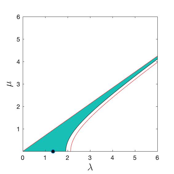
(a)

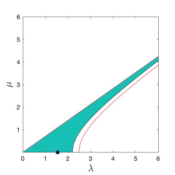
(b)

Figure 1. Region of modulational instability (shaded area) for (5.8). The corresponding region for the NLS equation is the extension represented by a red curve. The black dot represents the mode associated with maximum growth. Left panel: $(B_{0},k_{0})=(0.003,10)$. Right panel: $(B_{0},k_{0})=(0.0035,10)$.

7. Numerical results

We present numerical results to illustrate the performance of our Hamiltonian approach in the context of modulational instability of Stokes waves. We first present a theoretical analysis and then show some numerical simulations in comparison to other models.

7.1. Stability of Stokes waves

Equation (5.8) admits a uniform solution of the form

$$u_{0}(t)=B_{0}e^{-i(\omega_{0}+\varepsilon^{2}k_{0}^{3}B_{0}^{2})t}\,,$$

representing a progressive Stokes wave ($B_{0}$ being a positive real constant). Such a solution is known to be linearly unstable with respect to sideband perturbations, which is referred to as modulational or Benjamin–Feir (BF) instability. We provide a version of this analysis based on (5.8) for the three-dimensional problem.

Inserting a perturbation of the form

$$u({\rm X},t)=u_{0}(t)\big{[}1+B({\rm X},t)\big{]}\,,$$

where

$$B({\rm X},t)=B_{1}e^{\Omega t+i(\lambda X+\mu Y)}+B_{2}e^{\overline{\Omega}t-i(\lambda X+\mu Y)}\,,$$

and $B_{1},B_{2}$ are complex coefficients, we find that the condition $\operatorname{Re}(\Omega)\neq 0$ for instability implies

$$\left(\frac{\lambda^{2}}{2}-\mu^{2}\right)\left[2k_{0}^{2}B_{0}^{2}\left(k_{0}-\varepsilon\frac{\lambda^{2}}{\sqrt{\lambda^{2}+\mu^{2}}}\right)-\frac{\omega_{0}}{4k_{0}^{2}}\left(\frac{\lambda^{2}}{2}-\mu^{2}\right)\right]>0\,.$$ (7.1)

This is a tedious but straightforward calculation for which we skip the details. We refer the reader to [9, 22] for similar calculations.

Figure 1 shows instability regions in the $(\lambda,\mu)$-plane as predicted by condition (7.1) for $k_{0}=10$ and two different amplitudes $B_{0}=0.003$ and $0.0035$. Hereafter, all the variables are rescaled to absorb $\varepsilon$ back into their definition, and all the equations are non-dimensionalized so that $g=1$. These two plots correspond to wave steepnesses $\varepsilon=k_{0}A_{0}=0.075$ and $0.088$ respectively, based on the relationship

$$B_{0}=A_{0}\sqrt[4]{\frac{g}{4k_{0}}}\,,$$

between the envelope amplitude $B_{0}$ and the surface amplitude $A_{0}$ according to (2.8). In both cases, we see that the instability region is unbounded, extending in the form of a narrow strip to higher wavenumbers from the origin. Maximum growth (strongest instability) is achieved at $\mu=0$ and $\lambda\simeq 1.5$ which is a longitudinal long-wave mode. The instability region for the NLS equation, if $\varepsilon=0$ in (7.1), turns out to be larger and its extent relative to the Dysthe prediction is represented by a red curve in Fig. 1.

7.2. Simulations and comparisons

To validate our Hamiltonian approach, we test it against the full water wave system (2.1) which is given more explicitly by

$$\partial_{t}\eta=G(\eta)\xi\,,\quad\partial_{t}\xi=-g\eta-\frac{1}{2}|\partial_{\rm x}\xi|^{2}+\frac{\big{(}G(\eta)\xi+\partial_{\rm x}\eta\cdot\partial_{\rm x}\xi\big{)}^{2}}{2(1+|\partial_{\rm x}\eta|^{2})}\,.$$ (7.2)

We also compare our model predictions to solutions of the classical (non-Hamiltonian) Dysthe equation

$$i\,\partial_{t}A = -\frac{i\omega_{0}}{2k_{0}}\partial_{x}A+\frac{\omega_{0}}{8k_{0}^{2}}\partial_{x}^{2}A-\frac{\omega_{0}}{4k_{0}^{2}}\partial_{y}^{2}A+\frac{1}{2}\omega_{0}k_{0}^{2}|A|^{2}A+\frac{i\omega_{0}}{16k_{0}^{3}}\partial_{x}^{3}A$$ (7.3)

$$-\frac{3i\omega_{0}}{8k_{0}^{3}}\partial_{x}\partial_{y}^{2}A-\frac{3i}{2}\omega_{0}k_{0}|A|^{2}\partial_{x}A-\frac{i}{4}\omega_{0}k_{0}A^{2}\partial_{x}\overline{A}+k_{0}A\,\partial_{x}\Phi\,,$$

where

$$\Phi=\frac{1}{2}\omega_{0}\partial_{x}|D|^{-1}|A|^{2}\,,\quad\partial_{x}\Phi=\frac{1}{2}\omega_{0}\partial_{x}^{2}|D|^{-1}|A|^{2}\,,$$

denote contributions from the wave-induced mean flow. In this formulation, the surface elevation and velocity potential are reconstructed perturbatively in terms of the Stokes expansion

$$\eta({\rm x},t) = \frac{1}{2\omega_{0}}\partial_{x}\Phi+\operatorname{Re}\!\left[Ae^{i\theta}+\frac{1}{2}(k_{0}A^{2}-iA\partial_{x}A)e^{2i\theta}+\frac{3}{8}k_{0}^{2}A^{3}e^{3i\theta}\right]+\ldots$$

$$\varphi({\rm x},z,t) = \Phi+\operatorname{Re}\!\left[\Big{(}-\frac{i\omega_{0}}{k_{0}}A+\frac{\omega_{0}}{2k_{0}^{2}}\partial_{x}A+\frac{3i\omega_{0}}{8k_{0}^{3}}\partial_{x}^{2}A\right.$$ (7.4)

$$\left.\qquad\qquad-\frac{i\omega_{0}}{4k_{0}^{3}}\partial_{y}^{2}A+\frac{i}{8}\omega_{0}k_{0}|A|^{2}A\Big{)}e^{i\theta}e^{k_{0}z}\right]+\ldots$$

up to third harmonics, as typically reported in the literature [10, 21]. The phase function is given by $\theta=k_{0}x-\omega_{0}t$. As mentioned earlier, Eqs. (7.3) and (7.2) are expressed in terms of unscaled variables for the purposes of this comparative study.

The full equations (7.2) are solved numerically following a high-order spectral approach [7]. They are discretized in space by a pseudo-spectral method based on the FFT. The computational domain spans $0\leq x\leq L_{x}$, $0\leq y\leq L_{y}$ with doubly periodic boundary conditions and is divided into a regular mesh of $N_{x}\times N_{y}$ collocation points. The DNO is computed via its series expansion (2.3) but, by analyticity, a small number $m$ of terms is sufficient to achieve highly accurate results. The number $m=4$ is selected based on previous extensive tests [12, 23]. Time integration of (7.2) is carried out in the Fourier space so that the linear terms can be solved exactly by the integrating factor technique. The nonlinear terms are integrated in time by using a 4th-order Runge–Kutta scheme with constant step $\Delta t$. The same numerical methods are applied to the envelope equations (5.8) and (7.3), as well as to their reconstruction formulas, with the same resolutions in space and time. In particular, Burgers equation (6.3) is integrated in $s$ by using the same step size $\Delta s=\Delta t$. As noted in our previous work on the two-dimensional problem [5], the additional cost of solving this relatively simple equation is insignificant.

Initial conditions of the form

$$u({\rm x},0)=B_{0}\big{[}1+0.1\cos(\lambda x)\cos(\mu y)\big{]}\,,\quad A({\rm x},0)=A_{0}\big{[}1+0.1\cos(\lambda x)\cos(\mu y)\big{]}\,,$$

are specified to define a perturbed Stokes wave for (5.8) and (7.3) respectively. Accordingly, it is important to ensure that appropriate initial conditions are prescribed for (7.2): Eqs. (6.3) with $u({\rm x},0)$ (resp. Eqs. (7.2) with $A({\rm x},0)$) are used when the full equations are compared to predictions from (5.8) (resp. (7.3)).

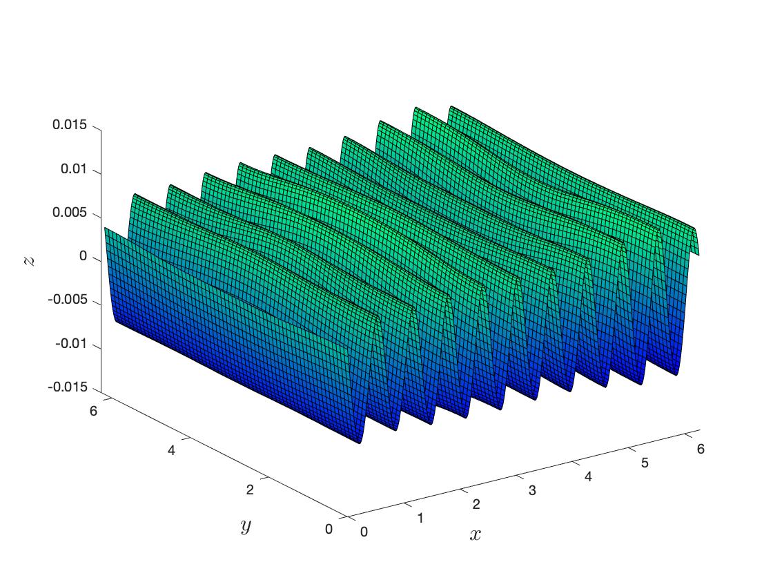
(a)

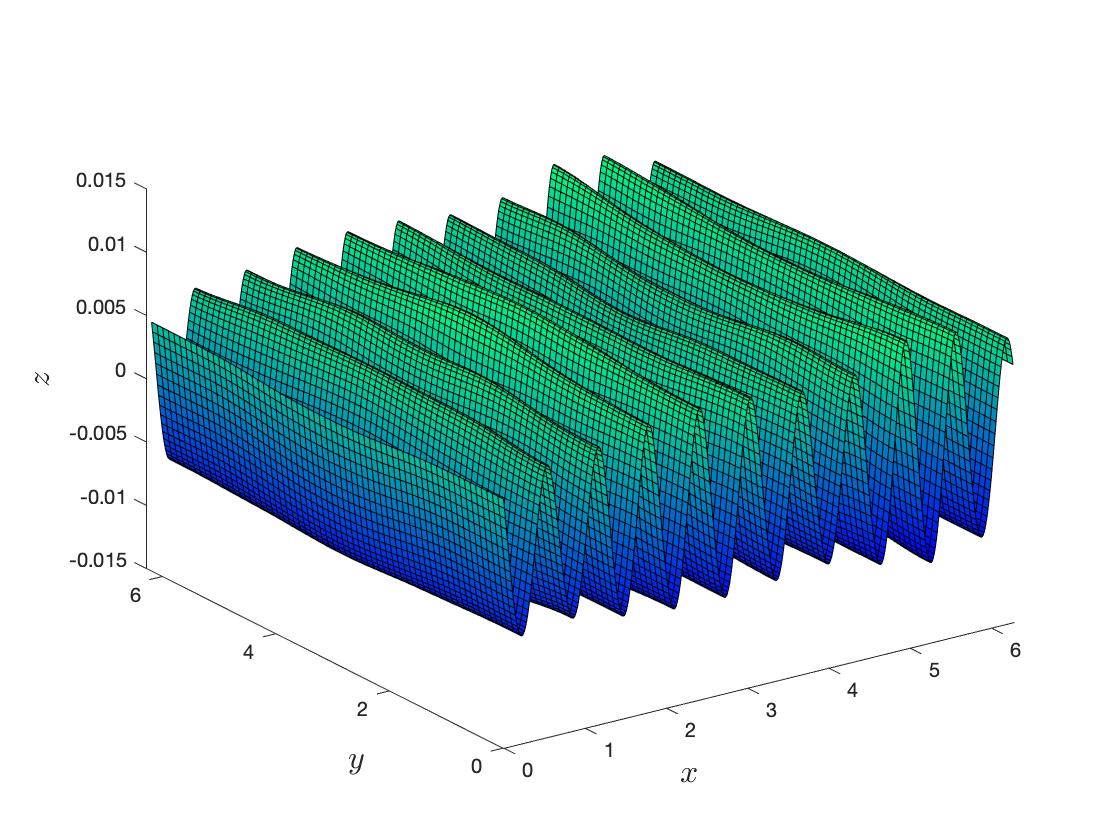
(b)

Figure 2. Surface elevation $\eta$ at $t=2500$ for $B_{0}=0.003$, $k_{0}=10$ and $(\lambda,\mu)=(1,1)$. Left panel: Hamiltonian Dysthe equation. Right panel: fully nonlinear equations.

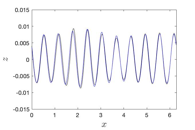
(a)

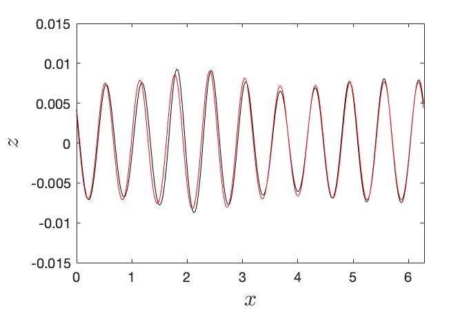
(b)

Figure 3. Comparison on $\eta$ between the fully and weakly nonlinear solutions in the cross-section $y=L_{y}/2$ at $t=2500$ for $B_{0}=0.003$, $k_{0}=10$ and $(\lambda,\mu)=(1,1)$. Left panel: Hamiltonian Dysthe equation in blue. Right panel: classical Dysthe equation in red. The black curve represents the fully nonlinear solution.

The following tests focus on the two cases considered in the previous stability analysis. The initial wave parameters are $k_{0}=10$, $B_{0}=0.003$ or $0.0035$, and $(\lambda,\mu)=(1,1)$ so that the initial condition is a Stokes wave under three-dimensional long-wave (i.e. sideband) perturbations. The computational domain is taken to be of size $L_{x}\times L_{y}=2\pi\times 2\pi$. The spatial and temporal resolutions are set to $\Delta x=0.012$ ($N_{x}=512$), $\Delta y=0.098$ ($N_{y}=64$) and $\Delta t=0.005$. This difference in resolution between $x$ and $y$ reflects the choice of $x$ as the preferred direction of wave propagation.

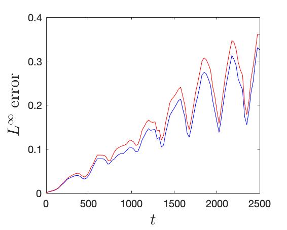
(a)

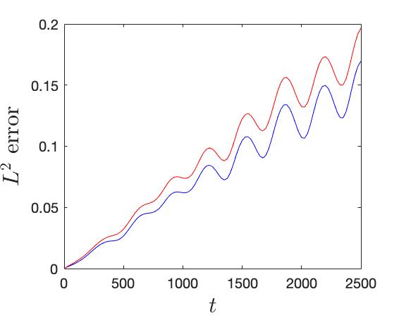
(b)

Figure 4. Relative errors on $\eta$ versus time between the fully and weakly nonlinear solutions for $B_{0}=0.003$, $k_{0}=10$ and $(\lambda,\mu)=(1,1)$. The blue curve represents the Hamiltonian Dysthe equation while the red curve represents the classical Dysthe equation. Left panel: $L^{\infty}$ error. Right panel: $L^{2}$ error.

For the first case with small initial data ($B_{0}=0.003$), we examine the wave dynamics over a long time up to $t=2500=\mathcal{O}(\varepsilon^{-3})$ given the initial steepness $\varepsilon=0.075$. This corresponds to the time scale over which the Dysthe approximation with such initial data is supposed to be valid. Figure 2 shows the full surface elevation $\eta$ at $t=2500$ as predicted from (5.8) and (7.2). A more direct comparison between these two solutions is reported in Fig. 3(a) along the cross-section $y=L_{y}/2$. A similar test for the classical Dysthe equation (7.3) is depicted in Fig. 3(b). Under such a mild disturbance, effects of modulational instability are not felt yet. In both cases, the wave profiles remain close to their initial configuration and, as a result, both plots look quite similar. A more quantitative assessment is provided in Fig. 4 which displays the time evolution of the relative $L^{\infty}$ and $L^{2}$ errors

$$\frac{\|\eta_{f}-\eta_{w}\|_{\infty}}{\|\eta_{f}\|_{\infty}}\,,\quad\frac{\|\eta_{f}-\eta_{w}\|_{2}}{\|\eta_{f}\|_{2}}\,,$$ (7.5)

on $\eta$ between the fully ($\eta_{f}$) and weakly ($\eta_{w}$) nonlinear solutions. The low values confirm that both Dysthe models perform very well in this case, with the predictions from (5.8) being slightly better than those from (7.3). This is consistent with results for the two-dimensional problem and is expected considering that the surface reconstruction for (5.8) is a non-perturbative procedure as opposed to the perturbative calculation for (7.3).

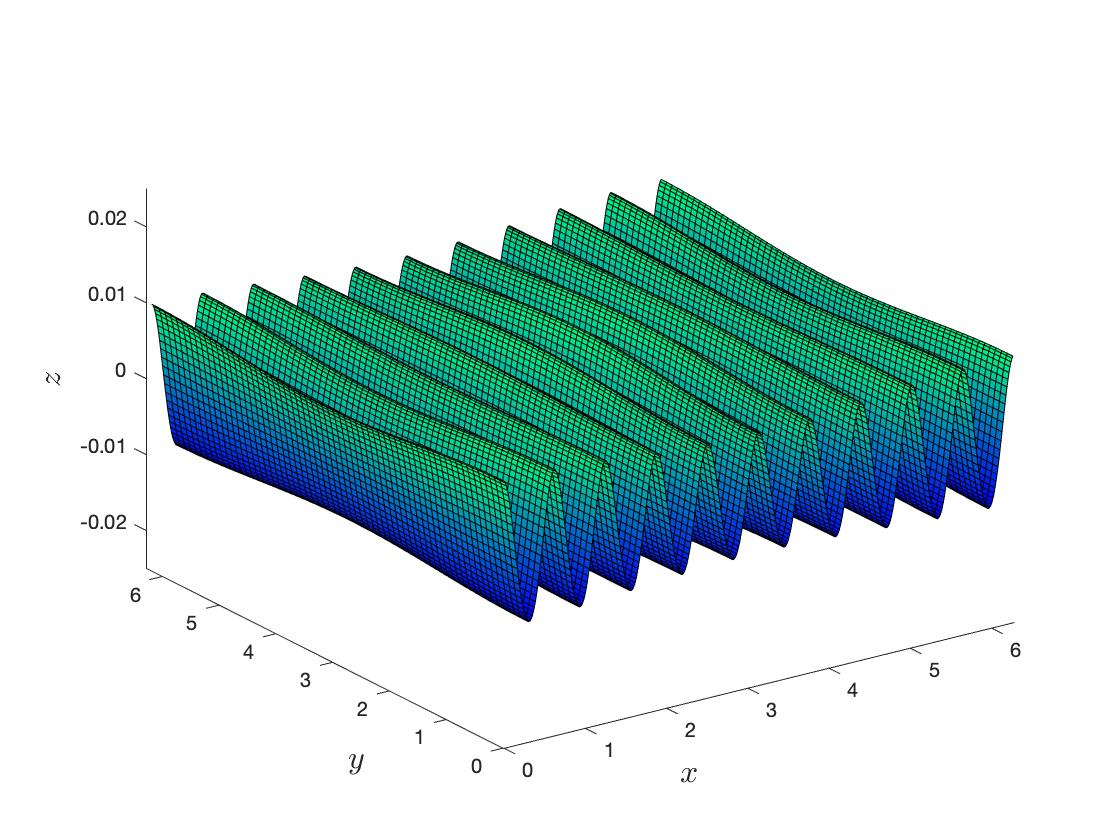
(a)

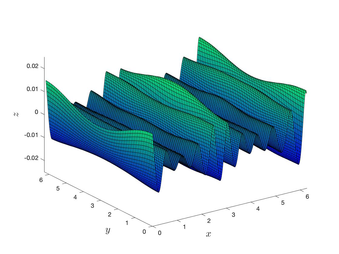
(b)

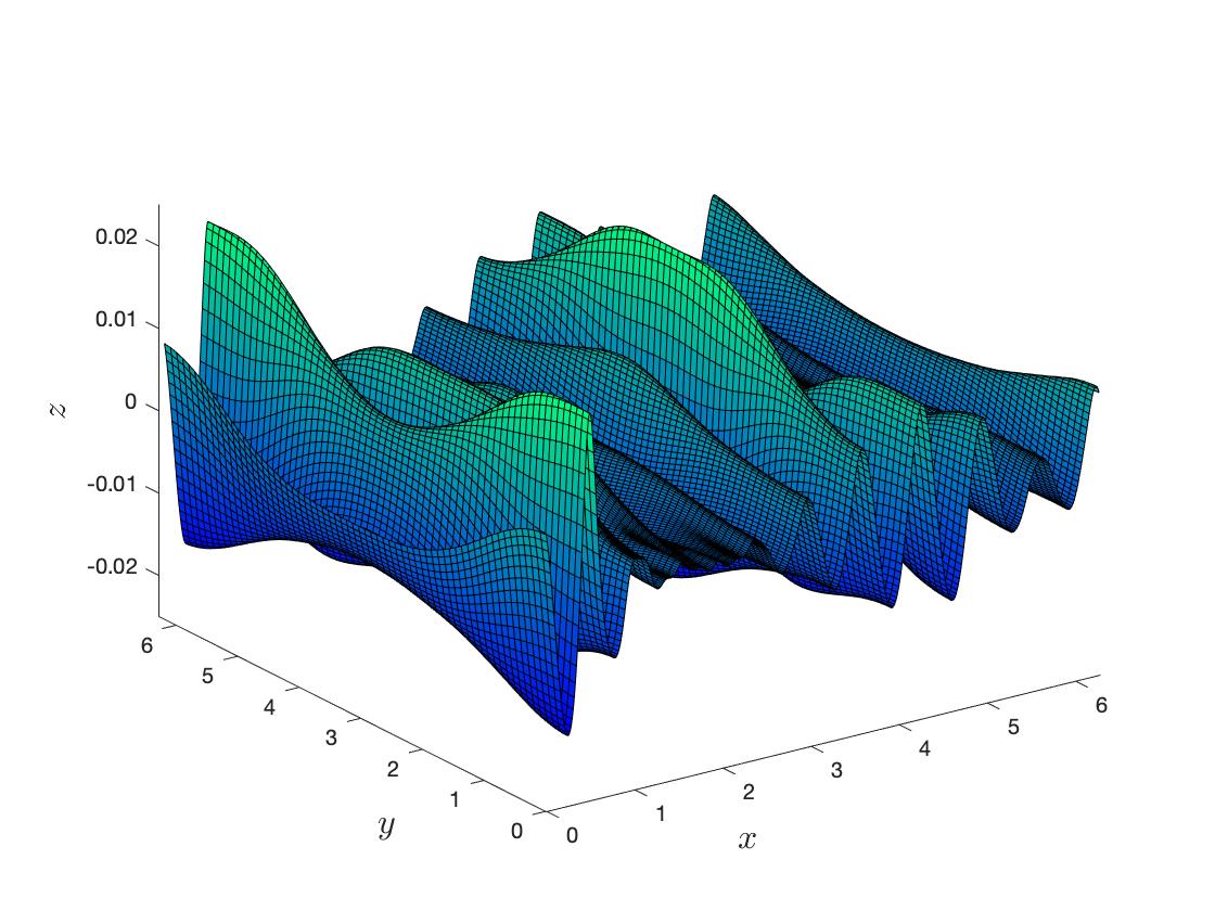
(c)

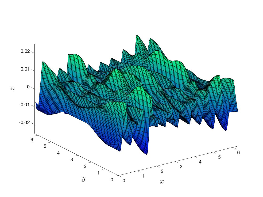
(d)

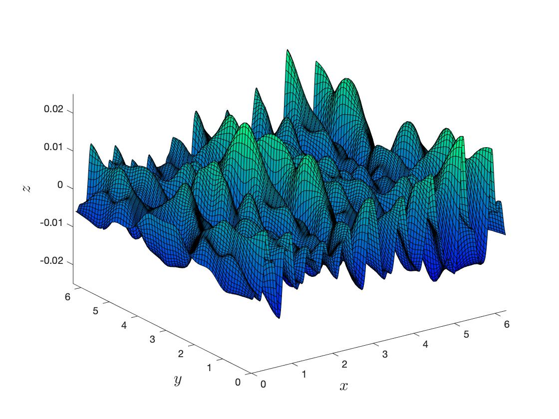
(e)

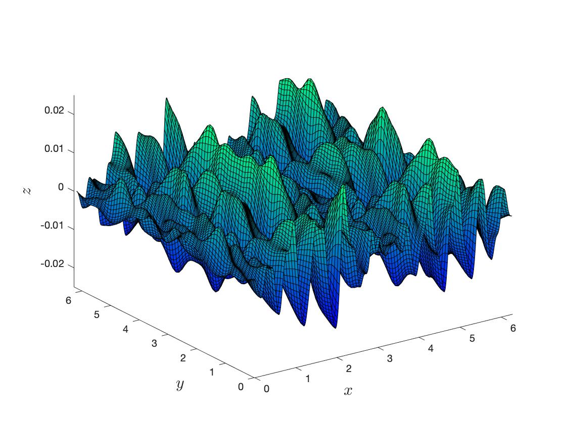
(f)

Figure 5. Surface elevation $\eta$ as predicted from the Hamiltonian Dysthe equation at (a) $t=0$, (b) $t=540$, (c) $t=680$, (d) $t=810$, (e) $t=930$, (f) $t=1000$ for $B_{0}=0.0035$, $k_{0}=10$ and $(\lambda,\mu)=(1,1)$.

The second case with larger initial data ($B_{0}=0.0035$, $\varepsilon=0.088$) is more prone to modulational instability. Snapshots of the full surface elevation up to $t=1000$ are presented in Fig. 5. As expected, the Stokes wave becomes unstable under the incipient development of the longitudinal sideband mode $\lambda=1$ (and near mode $\lambda=2$) around $t=680$. However, unlike the two-dimensional situation where a quasi-recurrent cycle of modulation-demodulation typically takes place over a long time [5], these perturbations quickly trigger the excitation of higher sideband modes in both horizontal directions, leading to the emergence of an irregular short-crested wave field. This phenomenon is observed in both our weakly and fully nonlinear simulations, which is consistent with results from previous numerical studies [17, 19]. In particular, computations by McLean et al. [19] showed that three-dimensional instabilities become dominant when the wave steepness is sufficiently large. In the present modulational regime, the gradual excitation of higher modes during wave evolution may be anticipated based on the stability analysis from Sec. 7.1, which reveals that the instability region for three-dimensional perturbed Stokes waves is not confined to the first few modes but extends over a wide range in the $(\lambda,\mu)$-plane. The energy initially contained in low sidebands can leak to higher unstable modes, similar to the scenario reported by Martin and Yuen [18] in the context of the NLS equation. The resulting choppy sea appearance as illustrated in Fig. 5 at $t=930$ and $1000$ is an indication of the limited range of applicability of the narrowband approximation in this three-dimensional case, even for moderate initial steepnesses.

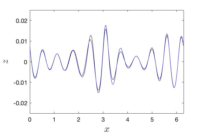
(a)

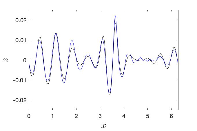
(b)

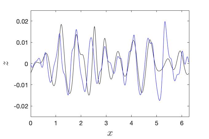
(c)

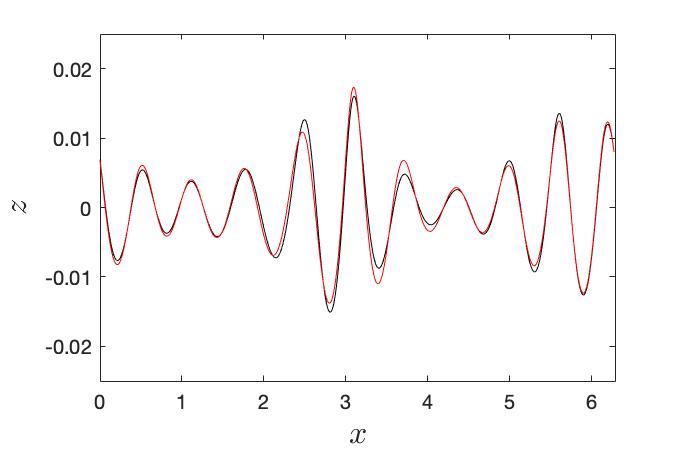
(d)

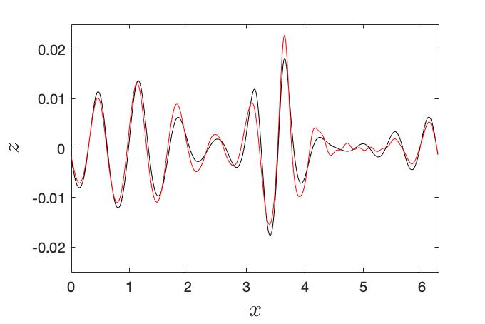
(e)

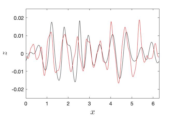
(f)

Figure 6. Comparison on $\eta$ between the fully and weakly nonlinear solutions in the cross-section $y=L_{y}/2$ at $t=540$, $680$, $1000$ (from left to right) for $B_{0}=0.0035$, $k_{0}=10$ and $(\lambda,\mu)=(1,1)$. Upper panels: Hamiltonian Dysthe equation in blue. Lower panels: classical Dysthe equation in red. The black curve represents the fully nonlinear solution.

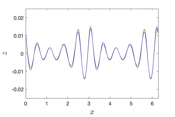
(a)

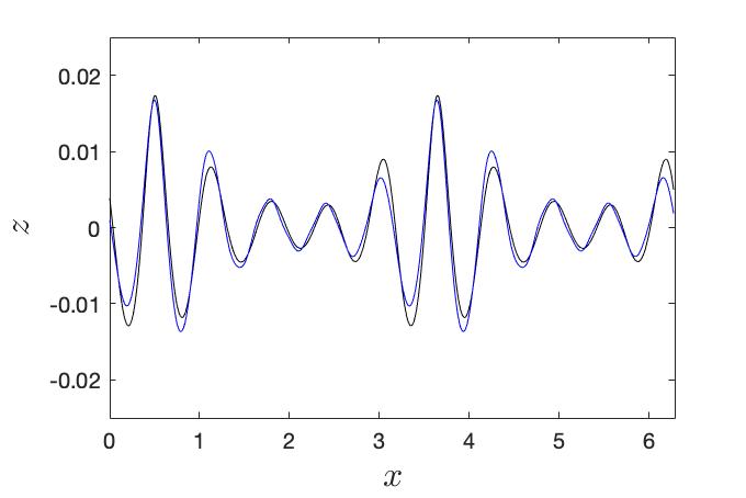
(b)

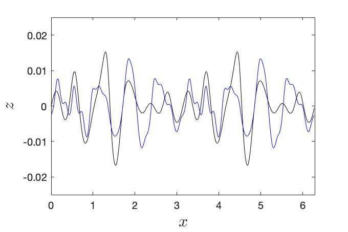
(c)

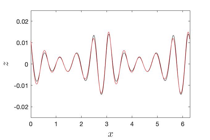
(d)

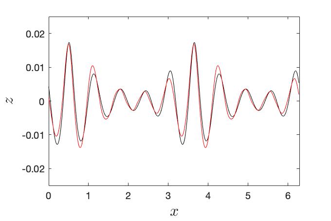
(e)

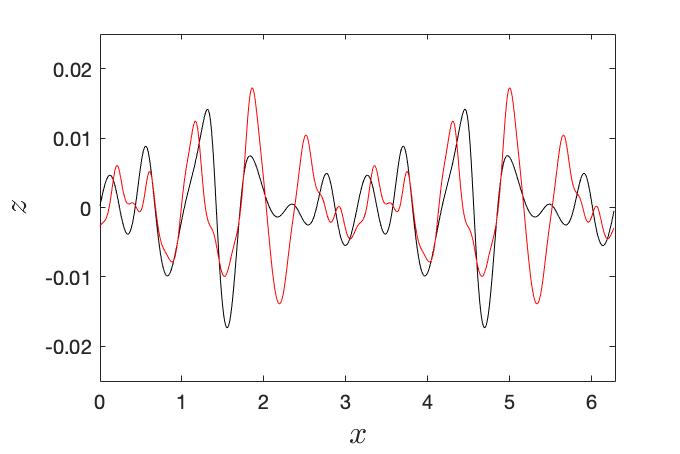
(f)

Figure 7. Comparison on $\eta$ between the fully and weakly nonlinear solutions in the cross-section $y=3L_{y}/4$ at $t=540$, $680$, $1000$ (from left to right) for $B_{0}=0.0035$, $k_{0}=10$ and $(\lambda,\mu)=(1,1)$. Upper panels: Hamiltonian Dysthe equation in blue. Lower panels: classical Dysthe equation in red. The black curve represents the fully nonlinear solution.

Comparison of (5.8) and (7.3) with (7.2) is given in Figs. 6 and 7 along the cross-sections $y=L_{y}/2$ and $3L_{y}/4$ respectively. Snapshots of $\eta$ at $t=540$ (early stage of BF instability), $t=680$ (around the time of BF maximum growth) and $t=1000$ (short-crested wave field) are presented, where we can clearly see the development of the longitudinal mode $\lambda=1$ and near mode $\lambda=2$ reaching a maximum amplitude of about $0.02$. As suspected earlier, discrepancies between the weakly and fully nonlinear solutions are quite pronounced at $t=1000$ along both cross-sections. This is especially true for the crest and trough heights, while there is still good agreement on the phase overall. Differences between the classical and Hamiltonian Dysthe solutions also become more noticeable as time goes by.

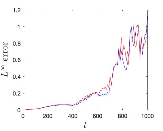
(a)

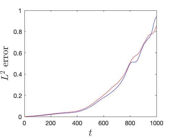
(b)

Figure 8. Relative errors on $\eta$ versus time between the fully and weakly nonlinear solutions for $B_{0}=0.0035$, $k_{0}=10$ and $(\lambda,\mu)=(1,1)$. The blue curve represents the Hamiltonian Dysthe equation while the red curve represents the classical Dysthe equation. Left panel: $L^{\infty}$ error. Right panel: $L^{2}$ error.

The relative $L^{\infty}$ and $L^{2}$ errors in Fig. 8 again tend to slightly favor our Hamiltonian approach. We note however that the situation seems to be reversed around $t=960$, with the errors for the classical Dysthe equation being lower from this point on. Having said that, this switch occurs at a late stage of modulational instability when errors are significant (near $80$%) and thus very likely either weakly nonlinear model is no longer suitable, as suggested in Figs. 6 and 7. An interpretation for this switch is that, because the Burgers equation automatically generates higher-order harmonics of the surface wave spectrum via nonlinear interactions, it may in turn excessively amplify errors as the validity of the Hamiltonian Dysthe equation deteriorates over time. From these plots, it seems that the time of validity is under $t=1000$ which contrasts with the expected time scale $\mathcal{O}(\varepsilon^{-3})\sim 1500$ based on the initial steepness. This value however is an overestimate in this case because the wave steepness increases as a result of modulational instability.

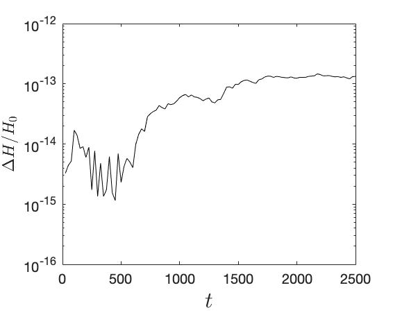
(a)

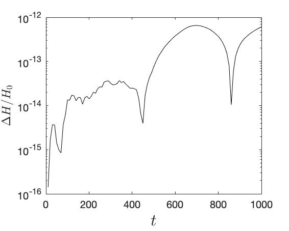
(b)

Figure 9. Relative error on $H$ versus time for the Hamiltonian Dysthe equation with $k_{0}=10$ and $(\lambda,\mu)=(1,1)$. Left panel: $B_{0}=0.003$. Right panel: $B_{0}=0.0035$.

Finally, the time evolution of the relative error

$$\frac{\Delta H}{H_{0}}=\frac{|H-H_{0}|}{H_{0}}\,,$$

on energy (5.7) associated with the Hamiltonian model (5.8) is illustrated in Fig. 9 for $B_{0}=0.003$ and $0.0035$. Double integrals in (5.7) and in the $L^{2}$ norm (7.5) are computed via the double trapezoidal rule over the periodic square $[0,2\pi]\times[0,2\pi]$. The reference value $H_{0}$ denotes the initial value of (5.7) at $t=0$. Overall, $H$ is very well conserved in both cases, despite a gradual loss of accuracy over time that is likely due to accumulation of numerical errors.

8. Conclusions

We propose a new Hamiltonian version of Dysthe’s equation for the nonlinear modulation of three-dimensional gravity waves on deep water. Starting from Zakharov’s formulation of the water wave problem, we perform a change to Birkhoff normal form that is devoid of non-resonant triads, together with a sequence of canonical transformations, in order to obtain a reduced system. The slowly varying wave envelope is introduced via a modulational Ansatz and the presence of multiple scales is handled through a homogenization procedure. The free surface is reconstructed by solving an auxiliary Hamiltonian system of differential equations. As a consequence, the entire solution process fits within a Hamiltonian framework. To validate this approach, we conduct numerical simulations on the modulational instability of Stokes waves and compare them to direct computations based on the full three-dimensional water wave system as well as to predictions from the classical Dysthe equation. Various wave conditions are examined and very good agreement is obtained within the range of validity of this approximation. In the future, we envision to extend these results to the finite-depth case for which a derivation of the third-order Birkhoff normal form is expected to be significantly more complicated.

Appendix A From physical to Fourier variables

We rewrite the Hamiltonian system (2.1) as

$$\partial_{t}\begin{pmatrix}\eta\\ \xi\\ \overline{\eta}\\ \overline{\xi}\end{pmatrix}=J_{1}\,\nabla H(\eta,\xi,\overline{\eta},\overline{\xi})=\begin{pmatrix}J&{O}_{2\times 2}\\ {O}_{2\times 2}&J\end{pmatrix}\begin{pmatrix}\partial_{\eta}H\\ \partial_{\xi}H\\ \partial_{\overline{\eta}}H\\ \partial_{\overline{\xi}}H\end{pmatrix}\,,$$

where $J$ is given by (2.1) and ${O}_{2\times 2}$ is the $2\times 2$ zero matrix. Denoting by $(\mathcal{F}\eta,\mathcal{F}\xi)$ the Fourier transforms of $(\eta,\xi)$, we define the transformation $\tau:v=(\eta,\xi,\overline{\eta},\overline{\xi})\mapsto w=(\overline{\mathcal{F}{\eta}},\overline{\mathcal{F}{\xi}},{\mathcal{F}{\eta}},{\mathcal{F}{\xi}})$ and write $\widetilde{H}(w)=H(v)$. Applying calculus rules of transformations [3], $w$ satisfies the system

$$\partial_{t}w=J_{2}\,\nabla\widetilde{H}(w)\,,$$ (A.1)

where $J_{2}=(\partial_{v}\tau)J_{1}(\partial_{v}\tau)^{*}$ and $(\partial_{v}\tau)^{*}$ is the adjoint matrix operator, such that

$$\partial_{v}\tau=\begin{pmatrix}{O}_{2\times 2}&{F}^{-1}\\ {F}&{O}_{2\times 2}\end{pmatrix}\,,\quad(\partial_{v}\tau)^{*}=\begin{pmatrix}{O}_{2\times 2}&{F}\\ {F}^{-1}&{O}_{2\times 2}\end{pmatrix}\,,$$

with $F=\mathcal{F}I_{2\times 2}$ and $F^{-1}=\mathcal{F}^{-1}I_{2\times 2}$. Computing the product of matrices,

$$J_{2}=\begin{pmatrix}F^{-1}JF^{-1}&O_{2\times 2}\\ O_{2\times 2}&FJF\end{pmatrix}=\begin{pmatrix}F^{-2}J&O_{2\times 2}\\ O_{2\times 2}&F^{2}J\end{pmatrix}\,.$$

Applying the matrix representation of $J_{2}$ to (A.1), we find

$$\partial_{t}\begin{pmatrix}\eta_{\rm k}\\ \xi_{\rm k}\end{pmatrix}=F^{2}J\begin{pmatrix}\partial_{\eta_{\rm k}}\widetilde{H}\\ \partial_{\xi_{\rm k}}\widetilde{H}\end{pmatrix}\iff\partial_{t}F^{-2}\begin{pmatrix}\eta_{\rm k}\\ \xi_{\rm k}\end{pmatrix}=\partial_{t}\begin{pmatrix}\eta_{-{\rm k}}\\ \xi_{-{\rm k}}\end{pmatrix}=J\begin{pmatrix}\partial_{\eta_{\rm k}}\widetilde{H}\\ \partial_{\xi_{\rm k}}\widetilde{H}\end{pmatrix}\,,$$

where we have used that $\mathcal{F}^{-2}(\eta_{\rm k},\xi_{\rm k})=(\eta_{-{\rm k}},\xi_{-{\rm k}})$. The water wave system in the Fourier space identifies to (2.5).

Appendix B Poisson bracket calculations

B.1. Useful identities

Lemma 6.

$$i\left\{\int F_{123}z_{1}z_{2}z_{3}\delta_{123}d{\rm k}_{123}\,,\int G_{456}\overline{z}_{-4}\overline{z}_{-5}\overline{z}_{-6}\delta_{456}d{\rm k}_{456}\right\}$$ (B.1)

$$=-\int(F_{123}+F_{312}+F_{231})(G_{456}+G_{645}+G_{564})z_{2}z_{3}\overline{z}_{-5}\overline{z}_{-6}\delta_{123}\delta_{456}\delta_{14}d{\rm k}_{1\ldots 6}\,,$$

$$\int F_{{\rm k}_{1}}^{{\rm k}_{2},{\rm k}_{3}}G_{{\rm k}_{4}}^{{\rm k}_{5},{\rm k}_{6}}z_{2}z_{3}\overline{z}_{-5}\overline{z}_{-6}\delta_{123}\delta_{456}\delta_{14}d{\rm k}_{1\ldots 6}=\int F_{-{\rm k}_{1}-{\rm k}_{2}}^{{\rm k}_{1},{\rm k}_{2}}G_{-{\rm k}_{3}-{\rm k}_{4}}^{{\rm k}_{3},{\rm k}_{4}}z_{1}z_{2}\overline{z}_{-3}\overline{z}_{-4}\delta_{1234}d{\rm k}_{1\ldots 4}\,.$$ (B.2)

Assuming that $F_{123}=F_{213}$ and $G_{456}=G_{546}$, then

$$i\left\{\int F_{123}z_{1}z_{2}\overline{z}_{-3}\delta_{123}d{\rm k}_{123}\,,\int G_{456}\overline{z}_{-4}\overline{z}_{-5}z_{6}\delta_{456}d{\rm k}_{456}\right\}$$ (B.3)

$$= \int(-4F_{123}G_{456}z_{2}\overline{z}_{-3}\overline{z}_{-5}z_{6}\delta_{123}\delta_{456}\delta_{14}+F_{123}G_{456}z_{1}z_{2}\overline{z}_{-4}\overline{z}_{-5}\delta_{123}\delta_{456}\delta_{36})d{\rm k}_{1\ldots 6}\,,$$

$$\int F_{{\rm k}_{1}}^{{\rm k}_{2},{\rm k}_{3}}G_{{\rm k}_{4}}^{{\rm k}_{5},{\rm k}_{6}}z_{2}\overline{z}_{-3}\overline{z}_{-5}z_{6}\delta_{123}\delta_{456}\delta_{14}d{\rm k}_{1\ldots 6}=\int F_{-{\rm k}_{1}-{\rm k}_{3}}^{{\rm k}_{1},{\rm k}_{3}}G_{-{\rm k}_{2}-{\rm k}_{4}}^{{\rm k}_{4},{\rm k}_{2}}z_{1}z_{2}\overline{z}_{-3}\overline{z}_{-4}\delta_{1234}d{\rm k}_{1\ldots 4}\,,$$ (B.4)

$$\int F_{{\rm k}_{1}}^{{\rm k}_{2},{\rm k}_{3}}G_{{\rm k}_{4}}^{{\rm k}_{5},{\rm k}_{6}}z_{1}z_{2}\overline{z}_{-4}\overline{z}_{-5}\delta_{123}\delta_{456}\delta_{36}d{\rm k}_{1\ldots 6}=\int F_{{\rm k}_{1}}^{{\rm k}_{2},-{\rm k}_{1}-{\rm k}_{2}}G_{{\rm k}_{3}}^{{\rm k}_{4},-{\rm k}_{3}-{\rm k}_{4}}z_{1}z_{2}\overline{z}_{-3}\overline{z}_{-4}\delta_{1234}d{\rm k}_{1\ldots 4}\,.$$ (B.5)

We only prove (B.1). The other identities are proved in a similar manner. Applying the Poisson bracket formula (2.11),

$$\left\{\int F_{123}z_{1}z_{2}z_{3}\delta_{123}d{\rm k}_{123}\,,\int G_{456}\overline{z}_{-4}\overline{z}_{-5}\overline{z}_{-6}\delta_{456}d{\rm k}_{456}\right\}$$

$$=-\frac{1}{i}\sum_{\begin{subarray}{c}(l,m,n)\in P(1,2,3)\\ (p,q,r)\in P(4,5,6)\end{subarray}}\int F_{123}G_{456}z_{l}z_{m}\overline{z}_{-p}\overline{z}_{-q}\delta_{123}\delta_{456}\delta_{14}d{\rm k}_{1\ldots 6}\,,$$

where the summation goes over the sets of all permutations $P$ of $(1,2,3)$ and $(4,5,6)$. We then apply index rearrangements to turn all integrals in the summation into those with monomial $z_{2}z_{3}\overline{z}_{-5}\overline{z}_{-6}$. For example, rearranging $(1,2,3)\to(2,3,1)$ and $(4,5,6)\to(5,6,4)$, we get

$$\int F_{123}G_{456}z_{1}z_{2}\overline{z}_{-4}\overline{z}_{-5}\delta_{123}\delta_{456}\delta_{36}d{\rm k}_{1\ldots 6}=\int F_{231}G_{564}z_{2}z_{3}\overline{z}_{-5}\overline{z}_{-6}\delta_{123}\delta_{456}\delta_{14}d{\rm k}_{1\ldots 6}\,.$$

B.2. Proof of Proposition 3

We look for terms of the form $zz\overline{z}\overline{z}$ in the Poisson bracket $\{K^{(3)},H^{(3)}\}$ with $H^{(3)}$ and $K^{(3)}$ given in (4.3)–(4.4). To distinguish between the indices associated to $K^{(3)}$ and $H^{(3)}$, we use $(1,2,3)$ for $K^{(3)}$ and $(4,5,6)$ for $H^{(3)}$. We have

$$i\,\{K^{(3)},H^{(3)}\}_{R}= \left\{\int\frac{A_{123}~{}z_{1}z_{2}z_{3}}{\omega_{1}+\omega_{2}+\omega_{3}}\delta_{123}d{\rm k}_{123}\,,\int A_{456}\overline{z}_{-4}\overline{z}_{-5}\overline{z}_{-6}\delta_{456}d{\rm k}_{456}\right\}$$

$$-\left\{\int\frac{A_{123}~{}\overline{z}_{-1}\overline{z}_{-2}\overline{z}_{-3}}{\omega_{1}+\omega_{2}+\omega_{3}}\delta_{123}d{\rm k}_{123}\,,\int A_{456}z_{4}z_{5}z_{6}\delta_{456}d{\rm k}_{456}\right\}$$

$$+\left\{\int\frac{A_{123}~{}z_{1}z_{2}\overline{z}_{-3}}{\omega_{1}+\omega_{2}-\omega_{3}}\delta_{123}d{\rm k}_{123}\,,\int A_{456}\overline{z}_{-4}\overline{z}_{-5}z_{6}\delta_{456}d{\rm k}_{456}\right\}$$

$$-\left\{\int\frac{A_{123}~{}\overline{z}_{-1}\overline{z}_{-2}z_{3}}{\omega_{1}+\omega_{2}-\omega_{3}}\delta_{123}d{\rm k}_{123}\,,\int A_{456}z_{4}z_{5}\overline{z}_{-6}\delta_{456}d{\rm k}_{456}\right\}\,.$$

The second and fourth lines can be modified using the antisymmetry property of the Poisson bracket and interchanging the indices $(1,2,3)$ and $(4,5,6)$:

$$i\,\{K^{(3)},H^{(3)}\}_{R}= \left\{\int\frac{A_{123}~{}z_{1}z_{2}z_{3}}{\omega_{1}+\omega_{2}+\omega_{3}}\delta_{123}d{\rm k}_{123}\,,\int A_{456}\overline{z}_{-4}\overline{z}_{-5}\overline{z}_{-6}\delta_{456}d{\rm k}_{456}\right\}$$ (B.6)

$$+\left\{\int A_{123}z_{1}z_{2}z_{3}\delta_{123}d{\rm k}_{123}\,,\int\frac{A_{456}~{}\overline{z}_{-4}\overline{z}_{-5}\overline{z}_{-6}}{\omega_{4}+\omega_{5}+\omega_{6}}\delta_{456}d{\rm k}_{456}\right\}$$

$$+\left\{\int\frac{A_{123}~{}z_{1}z_{2}\overline{z}_{-3}}{\omega_{1}+\omega_{2}-\omega_{3}}\delta_{123}d{\rm k}_{123}\,,\int A_{456}\overline{z}_{-4}\overline{z}_{-5}z_{6}\delta_{456}d{\rm k}_{456}\right\}$$

$$+\left\{\int A_{123}z_{1}z_{2}\overline{z}_{-3}\delta_{123}d{\rm k}_{123}\,,\int\frac{A_{456}\overline{z}_{-4}\overline{z}_{-5}z_{6}}{\omega_{4}+\omega_{5}-\omega_{6}}\delta_{456}d{\rm k}_{456}\right\}$$

$$:=i\,(R_{1}+R_{2}+R_{3}+R_{4})\,,$$

where we denote each line of (B.6) by $R_{1}$, $R_{2}$, $R_{3}$, $R_{4}$ respectively.

Step 1. We show that the coefficient ${\rm I}=R_{1}+R_{2}$. Using the identity (B.1), we get

$$R_{1} =\int\frac{A_{123}+A_{312}+A_{231}}{\omega_{1}+\omega_{2}+\omega_{3}}(A_{456}+A_{645}+A_{564})z_{2}z_{3}\overline{z}_{-5}\overline{z}_{-6}\delta_{123}\delta_{456}\delta_{14}d{\rm k}_{123456}\,.$$ (B.7)

From (4.2),

$$S_{123}=\sqrt[4]{g|{\rm k}_{1}||{\rm k}_{2}||{\rm k}_{3}|}~{}\ell_{{\rm k}_{1}}^{{\rm k}_{3}}\,,\quad A_{123}+A_{312}+A_{231}=\frac{S_{123}}{8\pi\sqrt{2}}(\ell_{{\rm k}_{1}}^{{\rm k}_{3}}+\ell_{{\rm k}_{1}}^{{\rm k}_{2}}+\ell_{{\rm k}_{2}}^{{\rm k}_{3}})\,.$$

To simplify the integral in (B.7), we use the identity (B.2) with

$$F_{{\rm k}_{1},{\rm k}_{2},{\rm k}_{3}}:=\frac{A_{123}+A_{312}+A_{231}}{\omega_{1}+\omega_{2}+\omega_{3}}\,,\quad G_{{\rm k}_{4},{\rm k}_{5},{\rm k}_{6}}:=A_{456}+A_{645}+A_{564}\,,$$

and obtain

$$R_{1}=\int{\rm I}_{A}z_{1}z_{2}\overline{z}_{-3}\overline{z}_{-4}\delta_{1234}d{\rm k}_{1234}\,,$$

$${\rm I}_{A}= ~{}\frac{g^{1/4}}{128\pi^{2}}\frac{\sqrt[4]{|{\rm k}_{1}||{\rm k}_{2}||{\rm k}_{3}||{\rm k}_{4}||{\rm k}_{1}+{\rm k}_{2}||{\rm k}_{3}+{\rm k}_{4}|}}{\omega_{{\rm k}_{1}}+\omega_{{\rm k}_{2}}+\omega_{{\rm k}_{1}+{\rm k}_{2}}}$$

$$\times(\ell_{{\rm k}_{1}}^{{\rm k}_{2}}+\ell_{{\rm k}_{1}+{\rm k}_{2}}^{-{\rm k}_{1}}+\ell_{{\rm k}_{1}+{\rm k}_{2}}^{-{\rm k}_{2}})(\ell_{{\rm k}_{3}}^{{\rm k}_{4}}+\ell_{{\rm k}_{3}+{\rm k}_{4}}^{-{\rm k}_{3}}+\ell_{{\rm k}_{3}+{\rm k}_{4}}^{-{\rm k}_{4}})\,.$$

We repeat these steps to compute $R_{2}$ (the second line of (B.6)) and find

$$R_{2}=\int{\rm I}_{B}z_{1}z_{2}\overline{z}_{-3}\overline{z}_{-4}\delta_{1234}d{\rm k}_{1234}\,,$$

$${\rm I}_{B}= ~{}\frac{g^{1/4}}{128\pi^{2}}\frac{\sqrt[4]{|{\rm k}_{1}||{\rm k}_{2}||{\rm k}_{3}||{\rm k}_{4}||{\rm k}_{1}+{\rm k}_{2}||{\rm k}_{3}+{\rm k}_{4}|}}{\omega_{{\rm k}_{3}}+\omega_{{\rm k}_{4}}+\omega_{{\rm k}_{3}+{\rm k}_{4}}}$$

$$\times(\ell_{{\rm k}_{1}}^{{\rm k}_{2}}+\ell_{{\rm k}_{1}+{\rm k}_{2}}^{-{\rm k}_{1}}+\ell_{{\rm k}_{1}+{\rm k}_{2}}^{-{\rm k}_{2}})(\ell_{{\rm k}_{3}}^{{\rm k}_{4}}+\ell_{{\rm k}_{3}+{\rm k}_{4}}^{-{\rm k}_{3}}+\ell_{{\rm k}_{3}+{\rm k}_{4}}^{-{\rm k}_{4}})\,.$$

Thus $R_{1}+R_{2}=\int{\rm I}\,z_{1}z_{2}\overline{z}_{-3}\overline{z}_{-4}\delta_{1234}d{\rm k}_{1234}$ where ${\rm I}={\rm I}_{A}+{\rm I}_{B}$ is given in (4.8).

Step 2. We show that the combination of $R_{3}$ and $R_{4}$ identifies to ${\rm II}+{\rm III}$. We apply the identity (B.3) and get

$$R_{3}= \int\frac{4A_{123}A_{456}}{\omega_{1}+\omega_{2}-\omega_{3}}z_{2}\overline{z}_{-3}\overline{z}_{-5}z_{6}\delta_{123}\delta_{456}\delta_{14}d{\rm k}_{123456}$$ (B.8)

$$-\int\frac{A_{123}A_{456}}{\omega_{1}+\omega_{2}-\omega_{3}}z_{1}z_{2}\overline{z}_{-4}\overline{z}_{-5}\delta_{123}\delta_{456}\delta_{36}d{\rm k}_{123456}\,.$$

To further simplify the RHS, we turn all its monomials into $z_{1}z_{2}\overline{z}_{-3}\overline{z}_{-4}$. This can be done by using the identities (B.4) and (B.5). We now identify the terms on the RHS of (B.8)

$$R_{3} =\int({\rm II}_{A}+{\rm III}_{A})z_{1}z_{2}\overline{z}_{-3}\overline{z}_{-4}\delta_{1234}d{\rm k}_{1234}\,,$$

where ${\rm II}_{A}$ comes from the first term in (B.8),

$${\rm II}_{A}= ~{}\frac{g^{1/4}}{32\pi^{2}}\frac{\sqrt[4]{|{\rm k}_{1}||{\rm k}_{2}||{\rm k}_{3}||{\rm k}_{4}||{\rm k}_{1}+{\rm k}_{3}||{\rm k}_{2}+{\rm k}_{4}|}}{\omega_{{\rm k}_{1}}+\omega_{{\rm k}_{1}+{\rm k}_{3}}-\omega_{{\rm k}_{3}}}$$

$$\times(\ell_{{\rm k}_{1}}^{{\rm k}_{3}}+\ell_{{\rm k}_{1}+{\rm k}_{3}}^{-{\rm k}_{3}}-\ell_{{\rm k}_{1}+{\rm k}_{3}}^{-{\rm k}_{1}})(\ell_{{\rm k}_{4}}^{{\rm k}_{2}}+\ell_{{\rm k}_{2}+{\rm k}_{4}}^{-{\rm k}_{2}}-\ell_{{\rm k}_{2}+{\rm k}_{4}}^{-{\rm k}_{4}})\,,$$

and ${\rm III}_{A}$ from the second term in (B.8),

$${\rm III}_{A}= -\frac{g^{1/4}}{128\pi^{2}}\frac{\sqrt[4]{|{\rm k}_{1}||{\rm k}_{2}||{\rm k}_{3}||{\rm k}_{4}||{\rm k}_{1}+{\rm k}_{2}||{\rm k}_{3}+{\rm k}_{4}|}}{\omega_{{\rm k}_{1}}+\omega_{{\rm k}_{2}}-\omega_{{\rm k}_{1}+{\rm k}_{2}}}$$

$$\times(\ell_{{\rm k}_{1}+{\rm k}_{2}}^{-{\rm k}_{1}}+\ell_{{\rm k}_{1}+{\rm k}_{2}}^{-{\rm k}_{2}}-\ell_{{\rm k}_{1}}^{{\rm k}_{2}})(\ell_{{\rm k}_{3}+{\rm k}_{4}}^{-{\rm k}_{3}}+\ell_{{\rm k}_{3}+{\rm k}_{4}}^{-{\rm k}_{4}}-\ell_{{\rm k}_{3}}^{{\rm k}_{4}})\,.$$

We repeat these steps to compute $R_{4}$ (fourth line in (B.6)) and obtain

$$R_{4} =\int({\rm II}_{B}+{\rm III}_{B})z_{1}z_{2}\overline{z}_{-3}\overline{z}_{-4}\delta_{1234}d{\rm k}_{1234}\,,$$

where

$${\rm II}_{B}= ~{}\frac{g^{1/4}}{32\pi^{2}}\frac{\sqrt[4]{|{\rm k}_{1}||{\rm k}_{2}||{\rm k}_{3}||{\rm k}_{4}||{\rm k}_{1}+{\rm k}_{3}||{\rm k}_{2}+{\rm k}_{4}|}}{\omega_{{\rm k}_{4}}+\omega_{{\rm k}_{2}+{\rm k}_{4}}-\omega_{{\rm k}_{2}}}$$

$$\times(\ell_{{\rm k}_{1}}^{{\rm k}_{3}}+\ell_{{\rm k}_{1}+{\rm k}_{3}}^{-{\rm k}_{3}}-\ell_{{\rm k}_{1}+{\rm k}_{3}}^{-{\rm k}_{1}})(\ell_{{\rm k}_{4}}^{{\rm k}_{2}}+\ell_{{\rm k}_{2}+{\rm k}_{4}}^{-{\rm k}_{2}}-\ell_{{\rm k}_{2}+{\rm k}_{4}}^{-{\rm k}_{4}})\,,$$

and ${\rm III}_{B}$ comes from the second term in (B.8),

$${\rm III}_{B}= -\frac{g^{1/4}}{128\pi^{2}}\frac{\sqrt[4]{|{\rm k}_{1}||{\rm k}_{2}||{\rm k}_{3}||{\rm k}_{4}||{\rm k}_{1}+{\rm k}_{2}||{\rm k}_{3}+{\rm k}_{4}|}}{\omega_{{\rm k}_{3}}+\omega_{{\rm k}_{4}}-\omega_{{\rm k}_{3}+{\rm k}_{4}}}$$

$$\times(\ell_{{\rm k}_{1}+{\rm k}_{2}}^{-{\rm k}_{1}}+\ell_{{\rm k}_{1}+{\rm k}_{2}}^{-{\rm k}_{2}}-\ell_{{\rm k}_{1}}^{{\rm k}_{2}})(\ell_{{\rm k}_{3}+{\rm k}_{4}}^{-{\rm k}_{3}}+\ell_{{\rm k}_{3}+{\rm k}_{4}}^{-{\rm k}_{4}}-\ell_{{\rm k}_{3}}^{{\rm k}_{4}})\,.$$

Thus $R_{3}+R_{4}=\int({\rm II}_{A}+{\rm II}_{B}+{\rm III}_{A}+{\rm III}_{B})z_{1}z_{2}\overline{z}_{-3}\overline{z}_{-4}\delta_{1234}d{\rm k}_{1234}$ where ${\rm II}_{A}+{\rm II}_{B}$ identifies to ${\rm II}$ in (4.9) and ${\rm III}_{A}+{\rm III}_{B}$ identifies to ${\rm III}$ in (4.10). This completes the proof.

References

• [1] U. Brinch-Nielsen and I. G. Jonsson, Fourth order evolution equations and stability analysis for Stokes waves on arbitrary water depth, Wave Motion, 8 (1986), pp. 455–472.
• [2] R. Coifman and Y. Meyer, Nonlinear harmonic analysis and analytic dependence, Proc. Sympos. Pure Math., 43 (1985), pp. 71–78.
• [3] W. Craig, P. Guyenne, and H. Kalisch, Hamiltonian long-wave expansions for free surfaces and interfaces, Commun. Pure Appl. Math., 58 (2005), pp. 1587–1641.
• [4] W. Craig, P. Guyenne, and C. Sulem, A Hamiltonian approach to nonlinear modulation of surface water waves, Wave Motion, 47 (2010), pp. 552–563.
• [5] W. Craig, P. Guyenne, and C. Sulem, Normal form transformations and Dysthe’s equation for the nonlinear modulation of deep-water gravity waves, Water Waves, 3 (2021), pp. 127–152.
• [6] W. Craig, P. Guyenne, and C. Sulem, The water wave problem and Hamiltonian transformation theory. In: T. Bodnár et al. (eds) Waves in Flows. Advances in Mathematical Fluid Mechanics. Birkhäuser, Basel, pp. 113–196.
• [7] W. Craig and C. Sulem, Numerical simulation of gravity waves, J. Comput. Phys., 108 (1993), pp. 73–83.
• [8] W. Craig and C. Sulem, Mapping properties of normal forms transformations for water waves, Boll. Unione Mat. Ital., 9 (2016), pp. 289–318.
• [9] K. B. Dysthe, Note on a modification to the nonlinear Schrödinger equation for application to deep water waves, Proc. R. Soc. Lond. A, 369 (1979), pp. 105–114.
• [10] O. Gramstad and K. Trulsen, Hamiltonian form of the modified nonlinear Schrödinger equation for gravity waves on arbitrary depth, J. Fluid Mech., 670 (2011), pp. 404–426.
• [11] P. Guyenne, A. Kairzhan, C. Sulem, and B. Xu, Spatial form of a Hamiltonian Dysthe equation for deep-water gravity waves, Fluids, 6 (2021), 103.
• [12] P. Guyenne and D. P. Nicholls, A high-order spectral method for nonlinear water waves over moving bottom topography, SIAM J. Sci. Comput., 30 (2007), pp. 81–101.
• [13] T. Hara and C. C. Mei, Frequency downshift in narrowbanded surface waves under the influence of wind, J. Fluid Mech., 230 (1991), pp. 429–477.
• [14] S. J. Hogan, The fourth-order evolution equation for deep-water gravity-capillary waves, Proc. R. Soc. Lond. A, 402 (1985), pp. 359–372.
• [15] V. P. Krasitskii, On reduced equations in the Hamiltonian theory of weakly nonlinear surface waves, J. Fluid Mech., 272 (1994), pp.1–20.
• [16] E. Lo and C. C. Mei, A numerical study of water-wave modulation based on a higher-order nonlinear Schrödinger equation, J. Fluid Mech., 150 (1985), pp. 395–416.
• [17] E. Lo and C. C. Mei, Slow evolution of nonlinear deep water waves in two horizontal directions: a numerical study, Wave Motion, 9 (1987), pp. 245–259.
• [18] D. U. Martin and H. C. Yuen, Quasi-recurring energy leakage in the two-space-dimensional nonlinear Schrödinger equation, Phys. Fluids, 23 (1980), pp. 881–883.
• [19] J. W. McLean, Y. C. Ma, D. U. Martin, P. G. Saffman, and H. C. Yuen, Three-dimensional instability of finite-amplitude water waves, Phys. Rev. Lett., 46 (1981), pp. 817–820.
• [20] A. Slunyaev and E. Pelinovsky, Numerical simulations of modulated waves in a higher-order Dysthe equation, Water Waves, 2 (2020), pp. 59–77.
• [21] K. Trulsen, Weakly nonlinear and stochastic properties of ocean wave fields. Application to an extreme wave event. In: J. Grue, K. Trulsen (eds) Waves in Geophysical Fluids. CISM International Centre for Mechanical Sciences, vol. 489. Springer, Vienna, pp. 49–106.
• [22] K. Trulsen, I. Kliakhandler, K. B. Dysthe, and M. G.Velarde, On weakly nonlinear modulation of waves on deep water, Phys. Fluids, 12 (2000), pp. 2432–2437.
• [23] L. Xu, and P. Guyenne, Numerical simulation of three-dimensional nonlinear water waves, J. Comput. Phys., 228 (2009), pp. 8446–8466.
• [24] V. E. Zakharov, Stability of periodic waves of finite amplitude on the surface of a deep fluid, J. Appl. Mech. Tech. Phys., 9 (1968), pp. 190–194.