Construction of energy density functional for arbitrary spin polarization using functional renormalization group

Abstract

We show an application of the functional-renormalization-group aided density functional theory to the homogeneous electron gas with arbitrary spin polarization, which gives the energy density functional in the local spin density approximation. The correlation energy per particle is calculated at arbitrary Wigner-Seitz radius $r_{\text{s}}$ and spin polarization $\zeta$. In the high-density region, our result shows good agreement with Monte Carlo (MC) data. The agreement with MC data is better in the case of small spin polarization, while the discrepancy increases as the spin polarization increases. The magnetic properties given by our numerical results are also discussed.

I Introduction

Density functional theory [1, 2, 3] is a powerful framework for many-body systems employed in various fields, including condensed matter physics, quantum chemistry, and nuclear physics. The accuracy of DFT depends on the energy density functional (EDF) [4], which returns the ground-state energy as a functional of the ground-state density. Although the Hohenberg–Kohn theorem [1] guarantees the existence of the exact EDF, it does not provide a microscopic way to derive EDF; hence its development is a long-standing problem.

A useful framework for the construction of EDF is the effective action formalism [5, 6, 7, 8]. In this formalism, Polonyi, Sailer, and Schwenk [9, 10] put forward an approach inspired by the functional renormalization group (FRG) [11, 12, 13, 14]. We refer to this approach as the functional-renormalization-group aided density functional theory (FRG-DFT). This approach is based on a functional differential equation, called flow equation, in a closed form of the effective action, which corresponds to the free-energy density functional multiplied by the temperature [5, 6, 7]. For such a closed form of equation, some systematic approximation methods were proposed [9, 15, 16, 17]. The FRG-DFT has been numerically applied to low-dimensional toy models [15, 16, 18, 17, 19, 20, 21] including a mimic of the nuclear systems [18, 19, 20], and, recently, applied to electronic systems [22, 23], where we achieved the first application to the two and three dimensional cases in the study of the homogeneous electron gas (HEG) and EDFs for electrons are constructed in the local density approximation.

In the previous works of the FRG-DFT [9, 10, 15, 16, 18, 17, 19, 20, 22, 23, 21], the EDF of total particle-number density has been studied. The Hohenberg–Kohn theorem guarantees that the ground-state properties are determined by the total particle-number density. However, the Kohn–Sham scheme [2], which is a commonly used method in DFT, has limited power when formulated based on the EDF of total particle number: Although it is suitable for accurate analysis of the ground-state energy and density, the calculations of other quantities are not always straightforward [24]. A way to extend Kohn–Sham scheme is introducing EDF depending on additional densities [25]; one of such generalizations is taking into account the particle-number densities of each spin component to describe the magnetic properties [26]. Such a formulation of EDF for multi-component systems can also be directly applied to analyses of nuclear matter, which is infinite system of nucleons composed of various components such as protons, neutrons, and hyperons [27, 28, 29, 30, 31, 32, 33, 34, 35, 36, 37]. In the context of the FRG-DFT, the EDF depending on the pairing density in addition to the particle-number density to describe superfluid systems was discussed in Ref. [38].

As for electron systems, a simple EDF of the particle-number densities of each spin component is that in the local spin density approximation (LSDA), in which the exchange–correlation part of the EDF $E_{\text{xc}}\left[\rho_{\uparrow},\rho_{\downarrow}\right]$ is approximated as

$$E_{\text{xc}}\left[\rho_{\uparrow},\rho_{\downarrow}\right]\approx\int d\bm{x}\,\left(\rho_{\uparrow}\left(\bm{x}\right)+\rho_{\downarrow}\left(\bm{x}\right)\right)\epsilon_{\text{xc}}\left(\rho_{\uparrow}\left(\bm{x}\right),\rho_{\downarrow}\left(\bm{x}\right)\right),$$ (1)

where $\epsilon_{\text{xc}}\left(\rho_{\uparrow},\rho_{\downarrow}\right)$ is the exchange–correlation energy per particle, i.e., energy density, of the HEG of densities of particles with up spin $\rho_{\uparrow}$ and down spin $\rho_{\downarrow}$. At some values of $\rho_{\uparrow}$ and $\rho_{\downarrow}$, $\epsilon_{\text{xc}}\left(\rho_{\uparrow},\rho_{\downarrow}\right)$ has been obtained by the quantum Monte Carlo (QMC) calculations [39]. The QMC results are of significance not only for the construction of EDF [40, 41, 42] but also for the discussion of the properties of the HEG itself: In three dimensions, the existence of the phase transitions from paramagnetic phase to partially polarized or ferromagnetic phase and from ferromagnetic phase to Wigner crystal is predicted [43, 40, 44, 45, 46, 47, 48, 49, 50], although the predicted values of the transition densities are not always similar among these works. In two dimensions, the existence of the ferromagnetic phase is indicated by Refs. [51, 52, 53, 54, 55, 56], while it is suggested in Ref. [57] that the ferromagnetic phase is never stable compared to the paramagnetic one.

Since the QMC results are available only at few values of the densities due to the numerical cost, an empirical fitting function for the data is needed to obtain the value of EDF at arbitrary densities. In our previous work [23], we applied the FRG-DFT for the calculation of the correlation energy per particle in the spin-unpolarized (paramagnetic) case. We obtained the values at many values of density, namely 65536 points in the Wigner-Seitz radii $r_{\text{s}}\in\left[10^{-6}\,\mathrm{a.u.},100\,\mathrm{a.u.}\right)$, which enables us to determine EDF almost without the dependence on the fitting function.

In this paper, we extend our works [22, 23] to the case of arbitrary spin polarization $\zeta=\left(\rho_{\uparrow}-\rho_{\downarrow}\right)/\left(\rho_{\uparrow}+\rho_{\downarrow}\right)$. We give a formulation of the FRG-DFT with arbitrary spin polarization and dimensions. In the vertex expansion, which is a functional Taylor expansion around densities of interest, we give the flow equations for the density correlation functions at arbitrary order. The correlation energy per particle $\epsilon_{\text{c}}\left(r_{\text{s}},\zeta\right)$ is calculated at various $r_{\text{s}}$ and $\zeta$ in the three- and two-dimensional cases. In high-density region, our result shows good agreement with QMC data as a result of the fact that our correlation energy reproduces the exact behavior at high density given by the Gell-Mann–Brueckner (GB) resummation [58, 59]. The agreement with QMC data is better in the case of small spin polarization, while the discrepancy increases as the spin polarization increases, which causes the absence of the magnetic phase transition predicted by the QMC calculations.

We also discuss the interpolation function $f_{\text{c}}\left(r_{\text{s}},\zeta\right)$ defined by

$$f_{\text{c}}\left(r_{\text{s}},\zeta\right)=\frac{\epsilon_{\text{c}}\left(r_{\text{s}},\zeta\right)-\epsilon_{\text{c}}\left(r_{\text{s}},0\right)}{\epsilon_{\text{c}}\left(r_{\text{s}},1\right)-\epsilon_{\text{c}}\left(r_{\text{s}},0\right)},$$ (2)

which characterizes the $\zeta$ dependence of EDF. Since $\epsilon_{\text{c}}$ of only a few points $\zeta$ and $r_{\text{s}}$ are available in QMC calculation, interpolation with respect to $\zeta$ is demanded to obtain $\epsilon_{\text{c}}$ for arbitrary $\zeta$ to perform LSDA calculations, as similar to the interpolation with respect to $r_{\text{s}}$. A popular approach to determine $\epsilon_{\text{c}}\left(r_{\text{s}},\zeta\right)$ [26, 24] is the approximation $f_{\text{c}}\left(r_{\text{s}},\zeta\right)\approx f_{\text{x}}\left(\zeta\right)$ with the interpolation function for the exchange part $f_{\text{x}}\left(\zeta\right)$ given analytically. We find the deviation of $f_{\text{c}}\left(r_{\text{s}},\zeta\right)$ from $f_{\text{x}}\left(\zeta\right)$ at small $r_{\text{s}}$, where the FRG-DFT gives accurate results.

This paper is organized as follows: In Sec. II, we shall show an FRG-DFT formalism with arbitrary spin polarization and dimensions. The flow equations for the density correlation functions at arbitrary order are given. The expression for the correlation energy density is given in the case of the second-order truncation. It shall be analytically shown that the expression reproduces the GB resummation at high density. Our numerical results are presented in Sec. III. We show the result of the $r_{\text{s}}$ and $\zeta$ dependences of the correlation energy and discuss the magnetic properties given by our calculation. Section IV is devoted to the conclusion. In Appendix A, we give the derivation of Eqs. (15) and (16).

II Formalism

We consider the HEG with the homogeneous density $\overline{\rho}$ and the inverse temperature $\beta$ neutralized by the background ions with the same density. In order to apply our formalism to the three- and two-dimensional cases, we present the formulation in general spatial dimensions $D$. The action in the imaginary time formalism is given by

$$S\left[\psi,\psi^{*}\right] =S_{\text{el}}\left[\psi,\psi^{*}\right]+S_{\text{int}}\left[\psi,\psi^{*}\right],$$ (3a)

$$S_{\text{el}}\left[\psi,\psi^{*}\right] =\sum_{s}\int_{X}\psi_{s}^{*}\left(X_{\epsilon}\right)\left(\partial_{\tau}-\frac{1}{2}\nabla^{2}\right)\psi_{s}\left(X\right),$$

$$S_{\text{int}}\left[\psi,\psi^{*}\right] =\frac{1}{2}\iint_{X,\,X^{\prime}}U_{\scriptstyle{\text{{{{2b}}}}}}\left(X,X^{\prime}\right)\hat{\rho}_{\Delta}\left(X\right)\hat{\rho}_{\Delta}\left(X^{\prime}\right).$$ (3b)

Here, we have introduced the following notations: $X=\left(\tau,\bm{x}\right)$ with the imaginary time $\tau$ and spatial coordinate $\bm{x}$, the coordinate integral $\int_{X}=\int_{0}^{\beta}d\tau\int d\bm{x}$, $\hat{\rho}_{\Delta}\left(X\right)=\sum_{s}\hat{\rho}_{s}\left(X\right)-\overline{\rho}$ with the electron field $\psi_{s}\left(X\right)$ having spin $s$ and the electron density operator $\hat{\rho}_{s}\left(X\right)=\psi_{s}^{*}\left(X_{\epsilon}\right)\psi_{s}\left(X\right)$, and the simultaneous Coulomb interaction

$$U_{\text{2b}}\left(X,X^{\prime}\right)=\frac{1}{\left|\bm{x}-\bm{x}^{\prime}\right|}\delta\left(\tau-\tau^{\prime}\right).$$ (4)

The interaction term $S_{\text{int}}$ contains not only the electron-electron interaction term but also the electron-ion and ion-ion ones, which cancel each other, and consequently avoid the divergence from Hartree term in the infinite system [22]. Additionally, $X_{\epsilon}=\left(\tau+\epsilon,\bm{x}\right)$ with a positive infinitesimal $\epsilon$ has been introduced so that the corresponding Hamiltonian is normal ordered.

II.1 FRG-DFT flow equation

Following Refs. [9, 10], we analyze the evolution of the system with respect to the gradual change of the strength of the two-body Coulomb interaction [Eq. (4)]. For this purpose, the evolution parameter $\lambda\in\left[0,1\right]$ is attached to the interaction term $S_{\text{int}}\left[\psi,\psi^{*}\right]$ as follows:

$$S_{\lambda}\left[\psi,\psi^{*}\right]=S_{\text{el}}\left[\psi,\psi^{*}\right]+\lambda S_{\text{int}}\left[\psi,\psi^{*}\right].$$ (5)

This action becomes that for a non-interacting system at $\lambda=0$ and Eq. (3a) at $\lambda=1$.

Our previous works [22, 23] were focused on EDFs of the total density. In the present study, we extend our analysis to the case of EDFs for spin polarized systems. For this purpose, we introduce the generating functional for the correlation functions for $\hat{\rho}_{{\uparrow},\,{\downarrow}}\left(X\right)$:

$$Z_{\lambda}\left[J_{\uparrow},J_{\downarrow}\right]=\iint\mathcal{D}\psi\,\mathcal{D}\psi^{*}\,e^{-S_{\lambda}\left[\psi,\psi^{*}\right]+\sum_{s}\int_{X}\hat{\rho}_{s}\left(X\right)J_{s}\left(X\right)}.$$ (6)

The Legendre transformation of the generating functional for connected correlation functions $W_{\lambda}\left[J_{\uparrow},J_{\downarrow}\right]=\ln Z_{\lambda}\left[J_{\uparrow},J_{\downarrow}\right]$ gives the effective action:

$$\Gamma_{\lambda}\left[\rho_{\uparrow},\rho_{\downarrow}\right]= \,\sup_{J_{\uparrow},\,J_{\downarrow}}\left(\sum_{s}\int_{X}\rho_{s}\left(X\right)J_{s}\left(X\right)-W_{\lambda}\left[J_{\uparrow},J_{\downarrow}\right]\right)$$

$$= \,\sum_{s}\int_{X}\rho_{s}\left(X\right)J_{\text{sup},\,\lambda,\,s}\left[\rho_{\uparrow},\rho_{\downarrow}\right]\left(X\right)$$

$$\,-W_{\lambda}\left[J_{\text{sup},\,\lambda,\,{\uparrow}}\left[\rho_{\uparrow},\rho_{\downarrow}\right],J_{\text{sup},\,\lambda,\,{\downarrow}}\left[\rho_{\uparrow},\rho_{\downarrow}\right]\right].$$ (7)

Here, the external field $J_{\text{sup},\,\lambda,\,s}\left[\rho_{\uparrow},\rho_{\downarrow}\right]$, which gives the supremum of the first line of Eq. (II.1), satisfies

$$\frac{\delta W_{\lambda}\left[J_{\text{sup},\,\lambda,\,{\uparrow}}\left[\rho_{\uparrow},\rho_{\downarrow}\right],J_{\text{sup},\,\lambda,\,{\downarrow}}\left[\rho_{\uparrow},\rho_{\downarrow}\right]\right]}{\delta J_{s}\left(X\right)}=\rho_{s}\left(X\right).$$ (8)

The equilibrium densities $\rho_{\text{eq},\,s}\left(X\right)$ are determined through

$$\frac{\delta\Gamma_{\lambda}\left[\rho_{\text{eq},\,{\uparrow}},\rho_{\text{eq},\,{\downarrow}}\right]}{\delta\rho_{s}\left(X\right)}=\mu_{s},$$ (9)

where $\mu_{s}$ is the chemical potential of the electrons with the spin component $s$. In this case, Eq. (II.1) becomes

$$\Gamma_{\lambda}\left[\rho_{\text{eq},\,{\uparrow}},\rho_{\text{eq},\,{\downarrow}}\right]=\sum_{s}\mu_{s}\int_{X}\rho_{\text{eq},\,s}\left(X\right)-W_{\lambda}\left[\mu_{\uparrow},\mu_{\downarrow}\right],$$ (10)

because of $J_{\text{sup},\,\lambda,\,s}\left[\rho_{\text{eq},\,{\uparrow}},\rho_{\text{eq},\,{\downarrow}}\right]\left(X\right)=\mu_{s}$, which is obtained by the relation

$$\frac{\delta\Gamma_{\lambda}\left[\rho_{\uparrow},\rho_{\downarrow}\right]}{\delta\rho_{s}\left(X\right)}=J_{\text{sup},\,\lambda,\,s}\left[\rho_{\uparrow},\rho_{\downarrow}\right]\left(X\right).$$ (11)

Since $W_{\lambda}\left[\mu_{\uparrow},\mu_{\downarrow}\right]/\beta$ is the grand potential, $\Gamma_{\lambda}\left[\rho_{\text{eq},\,{\uparrow}},\rho_{\text{eq},\,{\downarrow}}\right]$ gives the free energy multiplied by $\beta$. At zero temperature, $\rho_{\text{eq},\,s}\left(X\right)$ and $\beta^{-1}\Gamma_{\lambda}\left[\rho_{\text{eq},\,{\uparrow}},\rho_{\text{eq},\,{\downarrow}}\right]$ are reduced to the ground-state density and energy, respectively. Therefore, the EDF of densities with each spin component is given as follows [15]:

$$E_{\lambda}\left[\rho_{\uparrow},\rho_{\downarrow}\right]=\lim_{\beta\to\infty}\beta^{-1}\Gamma_{\lambda}\left[\rho_{\uparrow},\rho_{\downarrow}\right],$$ (12)

which is a natural extension of the relation between EDF of total density and the effective action [5, 7].

The evolution of $\Gamma_{\lambda}\left[\rho_{\uparrow},\rho_{\downarrow}\right]$ can be described by a functional differential equation. This equation is derived in the same manner as EDF for total density [10, 15, 18, 19, 22] and reads

$$\partial_{\lambda}\Gamma_{\lambda}\left[\rho_{\uparrow},\rho_{\downarrow}\right]=\frac{1}{2}\iint_{X,\,X^{\prime}}U_{\text{2b}}\left(X-X^{\prime}\right)\left[\rho_{\Delta}\left(X\right)\rho_{\Delta}\left(X^{\prime}\right)+\sum_{s,\,s^{\prime}}\Gamma^{\text{({\hbox{ 2 }})}{-1}}_{\lambda,\,ss^{\prime}}\left[\rho_{\uparrow},\rho_{\downarrow}\right]\left(X_{\epsilon^{\prime}},X^{\prime}\right)-\sum_{s}\rho_{s}\left(X\right)\delta\left(\bm{x}-\bm{x}^{\prime}\right)\right].$$ (13)

Here, we have introduced $\rho_{\Delta}\left(X\right)=\sum_{s}\rho_{s}\left(X\right)-\overline{\rho}$ and the inverse of the second derivative of the effective action $\Gamma^{\text{($2$)}{-1}}_{\lambda,\,ss^{\prime}}\left[\rho_{\uparrow},\rho_{\downarrow}\right]\left(X,X^{\prime}\right)$ defined through the following relation:

$$\sum_{s^{\prime\prime}}\int_{X^{\prime\prime}}\Gamma^{\text{($2$)}{-1}}_{\lambda,\,ss^{\prime\prime}}\left[\rho_{\uparrow},\rho_{\downarrow}\right]\left(X,X^{\prime\prime}\right)\frac{\delta^{2}\Gamma_{\lambda}\left[\rho_{\uparrow},\rho_{\downarrow}\right]}{\delta\rho_{s^{\prime\prime}}\left(X^{\prime\prime}\right)\,\delta\rho_{s^{\prime}}\left(X^{\prime}\right)}$$

$$=\delta_{ss^{\prime}}\delta\left(X-X^{\prime}\right),$$ (14)

where $\delta\left(X-X^{\prime}\right)=\delta\left(\tau-\tau^{\prime}\right)\delta\left(\bm{x}-\bm{x}^{\prime}\right)$ with $X=\left(\tau,\bm{x}\right)$ and $X^{\prime}=\left(\tau^{\prime},\bm{x}^{\prime}\right)$.

II.2 Vertex expansion

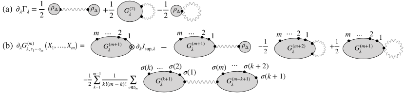
Figure 1: Diagrammatic representation of Eqs. (15) and (16). The wavy lines represent the two-body interaction $U_{\text{2b}}\left(X-X^{\prime}\right)$. The numbers $1$, $2$, …, $m$ attached to the diagrams of the correlation functions $G^{\text{($m+2$)}}_{\lambda}$, $G^{\text{($m+1$)}}_{\lambda}$, …stand for the sets of the coordinate and spin $\left(X_{1},s_{1}\right)$, $\left(X_{2},s_{2}\right)$, …, $\left(X_{m},s_{m}\right)$.

In principle, $\Gamma_{\lambda}\left[\rho_{\uparrow},\rho_{\downarrow}\right]$ is obtained by solving Eq. (13) with using the non-interacting system as the initial condition. In practice, however, some approximation for $\Gamma_{\lambda}\left[\rho_{\uparrow},\rho_{\downarrow}\right]$ is needed to solve Eq. (13) due to difficulty of direct numerical treatment of functional differential equations. Following Refs. [9, 10], we introduce the vertex expansion scheme, where a functional Taylor expansion at some densities of interest is applied and the differential equations for the Taylor coefficients of $\Gamma_{\lambda}\left[\rho_{\uparrow},\rho_{\downarrow}\right]$ are truncated at some order. As derived in Appendix A, these differential equations up to an arbitrary order read in terms of the density correlation functions as follows:

$$\partial_{\lambda}\Gamma_{\lambda}\left[\rho_{\uparrow},\rho_{\downarrow}\right]=\frac{1}{2}\iint_{X,\,X^{\prime}}U_{\text{2b}}\left(X-X^{\prime}\right)\left[\rho_{\Delta}\left(X\right)\rho_{\Delta}\left(X^{\prime}\right)+\sum_{s,\,s^{\prime}}G^{\text{($2$)}}_{\lambda,\,ss^{\prime}}\left(X_{\epsilon^{\prime}},X^{\prime}\right)-\sum_{s}\rho_{s}\left(X\right)\delta\left(\bm{x}-\bm{x}^{\prime}\right)\right],$$ (15)

$$\partial_{\lambda}G^{\text{($m$)}}_{\lambda,\,s_{1}\cdots s_{m}}\left(X_{1},\ldots,X_{m}\right)$$

$$=\sum_{s}\int_{X}G^{\text{($m+1$)}}_{\lambda,\,s,s_{1}\cdots s_{m}}\left(X,X_{1},\ldots,X_{m}\right)\partial_{\lambda}J_{\text{sup},\,\lambda,\,s}\left[\rho_{\uparrow},\rho_{\downarrow}\right]\left(X\right)$$

$$\quad-\frac{1}{2}\sum_{s}\iint_{X,\,X^{\prime}}U_{\text{2b}}\left(X,X^{\prime}\right)\left(\rho_{\Delta}\left(X\right)G^{\text{($m+1$)}}_{\lambda,\,ss_{1}\cdots s_{m}}\left(X^{\prime},X_{1},\ldots,X_{m}\right)+\rho_{\Delta}\left(X^{\prime}\right)G^{\text{($m+1$)}}_{\lambda,\,ss_{1}\cdots s_{m}}\left(X,X_{1},\ldots,X_{m}\right)\right)$$

$$\quad-\frac{1}{2}\sum_{s,\,s^{\prime}}\iint_{X,\,X^{\prime}}U_{\text{2b}}\left(X,X^{\prime}\right)\left(G^{\text{($m+2$)}}_{\lambda,\,ss^{\prime}s_{1}\cdots s_{m}}\left(X_{\epsilon^{\prime}},X^{\prime},X_{1},\ldots,X_{m}\right)-G^{\text{($m+1$)}}_{\lambda,\,ss_{1}\cdots s_{m}}\left(X,X_{1},\ldots,X_{m}\right)\delta_{ss^{\prime}}\delta\left(\bm{x}-\bm{x}^{\prime}\right)\vphantom{\sum_{k=1}^{m-1}}\right.$$

$$\qquad\left.+\sum_{k=1}^{m-1}\frac{1}{k!\,\left(m-k\right)!}\sum_{\sigma\in S_{m}}G^{\text{($k+1$)}}_{\lambda,\,ss_{\sigma\left(1\right)}\cdots s_{\sigma\left(k\right)}}\left(X,X_{\sigma\left(1\right)},\ldots,X_{\sigma\left(k\right)}\right)G^{\text{($m-k+1$)}}_{\lambda,\,s^{\prime}s_{\sigma\left(k+1\right)}\cdots s_{\sigma\left(m\right)}}\left(X^{\prime},X_{\sigma\left(k+1\right)},\ldots,X_{\sigma\left(m\right)}\right)\right),$$ (16)

where $m\geq 1$ is an integer, $S_{m}$ stands for the symmetry group of order $m$, and the $m$-point density correlation function is defined by

$$G^{\text{($m$)}}_{\lambda,\,s_{1}\cdots s_{m}}\left(X_{1},\ldots,X_{m}\right)$$

$$=\frac{\delta^{m}W_{\lambda}\left[J_{\text{sup},\,\lambda,\,{\uparrow}}\left[\rho_{\uparrow},\rho_{\downarrow}\right],J_{\text{sup},\,\lambda,\,{\downarrow}}\left[\rho_{\uparrow},\rho_{\downarrow}\right]\right]}{\delta J_{s_{1}}\left(X_{1}\right)\ldots\delta J_{s_{m}}\left(X_{m}\right)}.$$ (17)

The diagrammatic representation of Eqs. (15) and (16) is given in Fig. 1. Note that Eq. (16) at $m=1$ should be regarded as an equation describing the evolution of $J_{\text{sup},\,\lambda,\,s}\left[\rho_{\uparrow},\rho_{\downarrow}\right]\left(X\right)$ since the left-hand side is already determined by $\partial_{\lambda}G^{\text{($1$)}}_{\lambda,\,s_{1}}\left(X_{1}\right)=\partial_{\lambda}\rho_{s_{1}}\left(X_{1}\right)=0$ as obtained from Eq. (8).

II.3 Application to LSDA

Our purpose is the application to the LSDA EDF, which is described in terms of the effective action by

$$\Gamma_{\text{xc},\,\lambda}\left[\rho_{\uparrow},\rho_{\downarrow}\right]$$

$$\approx\int_{X}\left(\rho_{\uparrow}\left(X\right)+\rho_{\downarrow}\left(X\right)\right)\epsilon_{\text{xc},\,\lambda}\left(\rho_{\uparrow}\left(X\right),\rho_{\downarrow}\left(X\right)\right).$$ (18)

Here, $\Gamma_{\text{xc},\,\lambda}\left[\rho_{\uparrow},\rho_{\downarrow}\right]$ is given by the exchange–correlation part of the effective action

$$\Gamma_{\text{xc},\,\lambda}\left[\rho_{\uparrow},\rho_{\downarrow}\right]= \,\Gamma_{\lambda}\left[\rho_{\uparrow},\rho_{\downarrow}\right]-\Gamma_{\lambda=0}\left[\rho_{\uparrow},\rho_{\downarrow}\right]$$

$$\,-\frac{1}{2}\iint_{X,\,X^{\prime}}\lambda U_{\text{2b}}\left(X-X^{\prime}\right)\rho_{\Delta}\left(X\right)\rho_{\Delta}\left(X^{\prime}\right)$$

with the second and third terms of the right-hand side corresponding to the kinetic and Hartree terms, respectively, and $\epsilon_{\text{xc},\,\lambda}\left(\rho_{\uparrow},\rho_{\downarrow}\right)$ is the exchange–correlation energy per particle obtained in the homogeneous case with densities $\rho_{\uparrow}$ and $\rho_{\downarrow}$. Actually, Eq. (18) is reduced to the conventional definition of LSDA for EDF Eq. (1) as obtained from Eq. (12) with the density independent of the imaginary time $\rho_{s}\left(X\right)=\rho_{s}\left(\bm{x}\right)$. By putting Eq. (18) into Eq. (15), we have an equation to determine $\epsilon_{\text{xc},\,\lambda}\left(\rho_{\uparrow},\rho_{\downarrow}\right)$:

$$\int_{X}\left(\rho_{\uparrow}\left(X\right)+\rho_{\downarrow}\left(X\right)\right)\partial_{\lambda}\epsilon_{\text{xc},\,\lambda}\left(\rho_{\uparrow}\left(X\right),\rho_{\downarrow}\left(X\right)\right)$$

$$\approx\frac{1}{2}\iint_{X,\,X^{\prime}}U_{\text{2b}}\left(X-X^{\prime}\right)$$

$$\quad\times\left[\sum_{s,\,s^{\prime}}G^{\text{($2$)}}_{\lambda,ss^{\prime}}\left(X_{\epsilon^{\prime}},X^{\prime}\right)-\sum_{s}\rho_{s}\left(X\right)\delta\left(\bm{x}-\bm{x}^{\prime}\right)\right].$$ (19)

Particularly, Eq. (19) becomes exact at the homogeneous limit [60]. Given the homogeneous densities $\overline{\rho}_{s}$ satisfying $\overline{\rho}_{\uparrow}+\overline{\rho}_{\downarrow}=\overline{\rho}$, Eq. (19) is reduced to

$$\partial_{\lambda}\epsilon_{\text{xc},\,\lambda}\left(\overline{\rho}_{\uparrow},\overline{\rho}_{\downarrow}\right)$$

$$=\frac{1}{2\overline{\rho}}\int_{X}U_{\text{2b}}\left(X\right)\left[\sum_{s,\,s^{\prime}}G^{\text{($2$)}}_{\lambda,\,ss^{\prime}}\left(X_{\epsilon^{\prime}},0\right)-\overline{\rho}\delta\left(\bm{x}\right)\right].$$ (20)

Here, we have used $G^{\text{($2$)}}_{\lambda,\,ss^{\prime}}\left(X_{\epsilon^{\prime}},X^{\prime}\right)=G^{\text{($2$)}}_{\lambda,\,ss^{\prime}}\left(X_{\epsilon^{\prime}}-X^{\prime},0\right)$, which follows from the translational symmetry. Equation (20) is further reduced to the equation for the correlation part $\epsilon_{\text{c},\,\lambda}\left(\overline{\rho}_{\uparrow},\overline{\rho}_{\downarrow}\right)=\epsilon_{\text{xc},\,\lambda}\left(\overline{\rho}_{\uparrow},\overline{\rho}_{\downarrow}\right)-\epsilon_{\text{x},\,\lambda}\left(\overline{\rho}_{\uparrow},\overline{\rho}_{\downarrow}\right)$:

$$\partial_{\lambda}\epsilon_{\text{c},\,\lambda}\left(\overline{\rho}_{\uparrow},\overline{\rho}_{\downarrow}\right)$$

$$=\frac{1}{2\overline{\rho}}\sum_{s,\,s^{\prime}}\int_{X}U_{\text{2b}}\left(X\right)\left[G^{\text{($2$)}}_{\lambda,\,ss^{\prime}}\left(X_{\epsilon^{\prime}},0\right)-G^{\text{($2$)}}_{\lambda=0,ss^{\prime}}\left(X_{\epsilon^{\prime}},0\right)\right],$$ (21)

which is obtained by use of the expression for the exchange part $\epsilon_{\text{x},\,\lambda}\left(\overline{\rho}_{\uparrow},\overline{\rho}_{\downarrow}\right)$:

$$\epsilon_{\text{x},\,\lambda}\left(\overline{\rho}_{\uparrow},\overline{\rho}_{\downarrow}\right)$$

$$=\frac{\lambda}{2\overline{\rho}}\int_{X}U_{\text{2b}}\left(X\right)\left[\sum_{s,\,s^{\prime}}G^{\text{($2$)}}_{\lambda=0,\,ss^{\prime}}\left(X_{\epsilon^{\prime}},0\right)-\overline{\rho}\delta\left(\bm{x}\right)\right].$$ (22)

The analytic result of $\epsilon_{\text{x},\,\lambda}\left(\overline{\rho}_{\uparrow},\overline{\rho}_{\downarrow}\right)$ is known as follows [61, 62]:

$$\epsilon_{\text{x},\,\lambda}\left(\overline{\rho}_{\uparrow},\overline{\rho}_{\downarrow}\right)=-\frac{\lambda a_{D}}{r_{\text{s}}}\left[1+\left(2^{1/D}-1\right)f_{\text{x}}\left(\zeta\right)\right].$$ (23)

Here, $\zeta=\left(\overline{\rho}_{\uparrow}-\overline{\rho}_{\downarrow}\right)/\overline{\rho}$ is the spin polarization and $r_{\text{s}}$ is the Wigner–Seitz radius given by $r_{\text{s}}=\left(V_{D}\overline{\rho}\right)^{-1/D}$ with $V_{D=2}=\pi$ and $V_{D=3}=4\pi/3$ being the volume of a $D$-dimensional unit sphere. The interpolation function $f_{\text{x}}\left(\zeta\right)$ is defined by

$$f_{\text{x}}\left(\zeta\right)=\frac{\left(1+\zeta\right)^{\left(D+1\right)/D}+\left(1-\zeta\right)^{\left(D+1\right)/D}-2}{2^{\left(D+1\right)/D}-2}.$$ (24)

The coefficient $a_{D}$ is given by $a_{2}=4\sqrt{2}/\left(3\pi\right)$ and $a_{3}=3\left[3/\left(16\pi\right)\right]^{2/3}$. The momentum representation is a convenient choice for the homogeneous case. Then, Eqs. (16) and (21) are written as follows:

$$\partial_{\lambda}\epsilon_{\text{c},\,\lambda}\left(\overline{\rho}_{\uparrow},\overline{\rho}_{\downarrow}\right)=\frac{1}{2\overline{\rho}}\sum_{s,\,s^{\prime}}\int_{P}\tilde{U}\left(\bm{p}\right)e^{iP^{0}\epsilon^{\prime}}\left[\tilde{G}^{\text{($2$)}}_{\lambda,\,ss^{\prime}}\left(P\right)-\tilde{G}^{\text{($2$)}}_{\lambda=0,\,ss^{\prime}}\left(P\right)\right],$$ (25)

$$\partial_{\lambda}\tilde{G}^{\text{($m$)}}_{\lambda,\,s_{1}\ldots s_{m}}\left(P_{1},\ldots,P_{m-1}\right)$$

$$=\sum_{s}\tilde{G}^{\text{($m+1$)}}_{\lambda,\,ss_{1}\ldots s_{m}}\left(0,P_{1},\ldots,P_{m-1}\right)\partial_{\lambda}J_{\text{sup},\,\lambda,\,s}\left(\overline{\rho}_{\uparrow},\overline{\rho}_{\downarrow}\right)$$

$$\,\quad-\frac{1}{2}\int_{\bm{p}}\tilde{U}\left(\bm{p}\right)\left(\int_{P^{0}}e^{iP^{0}\epsilon^{\prime}}\sum_{s,\,s^{\prime}}\tilde{G}^{\text{($m+2$)}}_{\lambda,\,ss^{\prime}s_{1}\ldots s_{m}}\left(P,-P,P_{1},\ldots,P_{m-1}\right)-\sum_{s}\tilde{G}^{\text{($m+1$)}}_{\lambda,\,ss_{1}\ldots s_{m}}\left(0,P_{1},\ldots,P_{m-1}\right)\right)$$

$$\,\quad-\frac{1}{2}\sum_{k=1}^{m-1}\frac{1}{k!\,\left(m-k\right)!}\sum_{\sigma\in S_{m}}\tilde{U}\left(\sum_{i=1}^{k}\bm{p}_{\sigma\left(i\right)}\right)\sum_{s}\tilde{G}^{\text{($k+1$)}}_{\lambda,\,ss_{\sigma\left(1\right)}\ldots s_{\sigma\left(k\right)}}\left(-\sum_{i=1}^{k}P_{\sigma\left(i\right)},P_{\sigma\left(1\right)},\ldots,P_{\sigma\left(k-1\right)}\right)$$

$$\,\qquad\times\sum_{s^{\prime}}\tilde{G}^{\text{($m-k+1$)}}_{\lambda,\,s^{\prime}s_{\sigma\left(k+1\right)}\ldots s_{\sigma\left(m\right)}}\left(-\sum_{i=1}^{k}P_{\sigma\left(i\right)},P_{\sigma\left(k+1\right)},\ldots,P_{\sigma\left(m-1\right)}\right).$$ (26)

Here, we have introduced the four vector $P=\left(P^{0},\bm{p}\right)$ with the imaginary frequency $P^{0}$ and the spatial momentum $\bm{p}$ and $\int_{P}=\int dP^{0}/\left(2\pi\right)\int d\bm{p}/\left(2\pi\right)^{D}$. The Fourier components $\tilde{G}^{\text{($m$)}}_{\lambda,\,s_{1}\ldots s_{m}}\left(P_{1},\ldots,P_{m-1}\right)$ and $\tilde{U}\left(\bm{p}\right)$ are defined as follows:

$$\left(2\pi\right)^{4}\delta^{4}\left(\sum_{i=1}^{m}P_{i}\right)\tilde{G}^{\text{($m$)}}_{\lambda,\,s_{1}\ldots s_{m}}\left(P_{1},\ldots,P_{m-1}\right) =\int_{X_{1},\,\ldots,\,X_{m}}e^{i\sum_{i=1}^{m}P_{i}\cdot X_{i}}G^{\text{($m$)}}_{\lambda,\,s_{1}\ldots s_{m}}\left(X_{1},\ldots,X_{m}\right),$$

$$\tilde{U}\left(\bm{p}\right)=\int_{X}e^{iP\cdot X}U_{\text{2b}}\left(X\right) =\begin{cases}2\pi/\left|\bm{p}\right|&\text{($D=2$)},\\ 4\pi/\left|\bm{p}\right|^{2}&\text{($D=3$)}.\end{cases}$$ (27)

In Eq. (26), one of $P_{\sigma\left(1\right)}$, …, $P_{\sigma\left(m\right)}$ becomes $P_{m}$, which stands for $P_{m}=-\sum_{i=1}^{m-1}P_{i}$.

In this paper, we consider the vertex expansion up to the second order. The first and second order of Eq. (26) read

$$0= \,\sum_{s}\tilde{G}^{\text{($2$)}}_{\lambda,\,ss_{1}}\left(0\right)\partial_{\lambda}J_{\text{sup},\,\lambda,\,s}\left(\overline{\rho}_{\uparrow},\overline{\rho}_{\downarrow}\right)-\frac{1}{2}\int_{\bm{p}}\tilde{U}\left(\bm{p}\right)\left(\int_{P^{0}}e^{iP^{0}\epsilon^{\prime}}\sum_{s,\,s^{\prime}}\tilde{G}^{\text{($3$)}}_{\lambda,\,ss^{\prime}s_{1}}\left(P,-P\right)-\sum_{s}\tilde{G}^{\text{($2$)}}_{\lambda,\,ss_{1}}\left(0\right)\right),$$ (28)

$$\partial_{\lambda}\tilde{G}^{\text{($2$)}}_{\lambda,\,s_{1}s_{2}}\left(P_{1}\right)= \,\sum_{s}\tilde{G}^{\text{($3$)}}_{\lambda,\,ss_{1}s_{2}}\left(0,P_{1}\right)\partial_{\lambda}J_{\text{sup},\,\lambda,\,s}\left(\overline{\rho}_{\uparrow},\overline{\rho}_{\downarrow}\right)-\tilde{U}\left(\bm{p}_{1}\right)\sum_{s,\,s^{\prime}}\tilde{G}^{\text{($2$)}}_{\lambda,\,ss_{1}}\left(-P_{1}\right)\tilde{G}^{\text{($2$)}}_{\lambda,\,s^{\prime}s_{2}}\left(P_{1}\right)$$

$$\,-\frac{1}{2}\int_{\bm{p}}\tilde{U}\left(\bm{p}\right)\left(\int_{P^{0}}e^{iP^{0}\epsilon^{\prime}}\sum_{s,\,s^{\prime}}\tilde{G}^{\text{($4$)}}_{\lambda,\,ss^{\prime}s_{1}s_{2}}\left(P,-P,P_{1}\right)-\sum_{s}\tilde{G}^{\text{($3$)}}_{\lambda,\,ss_{1}s_{2}}\left(0,P_{1}\right)\right).$$ (29)

By canceling $\partial_{\lambda}J_{\text{sup},\,\lambda,\,s}\left(\overline{\rho}_{\uparrow},\overline{\rho}_{\downarrow}\right)$ in these equations, we have

$$\partial_{\lambda}\tilde{G}^{\text{($2$)}}_{\lambda,\,s_{1}s_{2}}\left(P_{1}\right)= \,-\tilde{U}\left(\bm{p}_{1}\right)\sum_{s,\,s^{\prime}}\tilde{G}^{\text{($2$)}}_{\lambda,\,ss_{1}}\left(-P_{1}\right)\tilde{G}^{\text{($2$)}}_{\lambda,\,s^{\prime}s_{2}}\left(P_{1}\right)+C_{\lambda,\,s_{1}s_{2}}\left(P_{1}\right),$$ (30)

$$C_{\lambda,\,s_{1}s_{2}}\left(P_{1}\right)= \,-\frac{1}{2}\int_{\bm{p}}\tilde{U}\left(\bm{p}\right)\int_{P^{0}}e^{iP^{0}\epsilon^{\prime}}$$

$$\,\times\sum_{s,\,s^{\prime}}\left(\tilde{G}^{\text{($4$)}}_{\lambda,\,ss^{\prime}s_{1}s_{2}}\left(P,-P,P_{1}\right)-\sum_{t,\,t^{\prime}}\tilde{G}^{\text{($3$)}}_{\lambda,\,ts_{1}s_{2}}\left(0,P_{1}\right)\left[\tilde{G}^{\text{($2$)}}_{\lambda}\left(0\right)\right]_{tt^{\prime}}^{-1}\tilde{G}^{\text{($3$)}}_{\lambda,\,ss^{\prime}t^{\prime}}\left(P,-P\right)\right),$$ (31)

where $\left[\tilde{G}^{\text{($2$)}}_{\lambda}\left(0\right)\right]_{tt^{\prime}}^{-1}$ is the inverse of $\tilde{G}^{\text{($2$)}}_{\lambda,\,tt^{\prime}}\left(0\right)$ with respect to the spin indices $t$ and $t^{\prime}$. As shown in Eq. (31), $C_{\lambda,\,s_{1}s_{2}}\left(P_{1}\right)$ is composed of higher-order correlation functions.

As in our previous works [22, 23], we ignore the $\lambda$ dependence of $C_{\lambda,\,s_{1}s_{2}}\left(P_{1}\right)$ as

$$C_{\lambda,\,s_{1}s_{2}}\left(P_{1}\right)\approx C_{\lambda=0,\,s_{1}s_{2}}\left(P_{1}\right).$$ (32)

Applying this approximation and summing up the spin indices, Eqs. (25) and (30) are rewritten as follows:

$$\partial_{\lambda}\epsilon_{\text{c},\,\lambda}\left(\overline{\rho}_{\uparrow},\overline{\rho}_{\downarrow}\right)= \,\frac{1}{2\overline{\rho}}\int_{P}\tilde{U}\left(\bm{p}\right)e^{iP^{0}\epsilon^{\prime}}$$

$$\,\times\left[\tilde{G}^{\text{($2$)}}_{\lambda}\left(P\right)-\tilde{G}^{\text{($2$)}}_{\lambda=0}\left(P\right)\right],$$ (33)

$$\partial_{\lambda}\tilde{G}^{\text{($2$)}}_{\lambda}\left(P_{1}\right)\approx \,-\tilde{U}\left(\bm{p}_{1}\right)\left[\tilde{G}^{\text{($2$)}}_{\lambda}\left(P_{1}\right)\right]^{2}+C_{\lambda=0}\left(P_{1}\right),$$ (34)

where we have introduced the total density correlation functions:

$$\tilde{G}^{\text{({\hbox{ m }})}}_{\lambda}\left(P_{1},\ldots,P_{m-1}\right)=\sum_{s_{1},\,\ldots,\,s_{m}}\tilde{G}^{\text{({\hbox{ m }})}}_{\lambda,\,s_{1}\ldots s_{m}}\left(P_{1},\ldots,P_{m-1}\right),$$ (35)

and

$$C_{\lambda=0}\left(P_{1}\right)=\sum_{s,\,s^{\prime}}C_{\lambda=0,ss^{\prime}}\left(P_{1}\right).$$ (36)

The solution of Eq. (34), which has the form of Riccati equation, can be obtained analytically with respect to $\lambda$. With this solution, the $\lambda$ integral in Eq. (33) is performed analytically. The solutions read

$$\tilde{G}^{\text{($2$)}}_{\lambda=1}\left(P\right)=\tilde{G}^{\text{($2$)}}_{\lambda=0}\left(P\right)\frac{1+\left(B_{P}/A_{P}\right)\tanh B_{P}}{1+\left(A_{P}/B_{P}\right)\tanh B_{P}},$$ (37)

$$\epsilon_{\text{c},\,\lambda=1}\left(\overline{\rho}_{\uparrow},\overline{\rho}_{\downarrow}\right)$$

$$=\frac{1}{2\overline{\rho}}\int_{P}\left[\ln\left(\cosh B_{P}+\frac{A_{P}}{B_{P}}\sinh B_{P}\right)-A_{P}\right],$$ (38)

where

$$A_{P} =\tilde{U}\left(\bm{p}\right)\tilde{G}^{\text{($2$)}}_{\lambda=0}\left(P\right),$$ (39a)

$$B_{P} =\sqrt{\tilde{U}\left(\bm{p}\right)C_{\lambda=0}\left(P\right)}.$$ (39b)

The quantity $C_{\lambda=0}\left(P_{1}\right)$ is given by the density correlation functions in the non-interacting case $\tilde{G}^{\text{($m$)}}_{\lambda=0,\,s_{1}\ldots s_{m}}\left(P_{1},\ldots,P_{m-1}\right)$:

$$\tilde{G}^{\text{($m$)}}_{\lambda=0,\,s_{1}\ldots s_{m}}\left(P_{1},\ldots,P_{m-1}\right)$$

$$=-\sum_{\sigma\in S_{m-1}}\int_{P^{\prime}}\prod_{k=0}^{m-1}\tilde{G}_{\text{F},s_{\sigma\left(k\right)}s_{\sigma\left(k+1\right)}}\left(\sum_{i=1}^{k}P_{\sigma\left(i\right)}+P^{\prime}\right),$$ (40)

where $\tilde{G}_{\text{F},ss^{\prime}}\left(P\right)$ is the propagator of the free fermion defined by

$$\tilde{G}_{\text{F},ss^{\prime}}\left(P=\left(\omega,\bm{p}\right)\right) =\delta_{ss^{\prime}}\tilde{G}_{\text{F}}\left(p_{\text{F},s};P=\left(\omega,\bm{p}\right)\right)$$

$$=\delta_{ss^{\prime}}\frac{e^{i\omega\epsilon}}{i\omega-\xi_{s}\left(\bm{p}\right)}$$ (41)

with $\xi_{s}\left(\bm{p}\right)=\bm{p}^{2}/2-p_{\text{F},s}^{2}/2$ and the Fermi momentum $p_{\text{F},s}=2\pi\left(\overline{\rho}_{s}/V_{D}\right)^{1/D}$. In Eq. (40), $\sigma\left(0\right)$ is defined by $\sigma\left(0\right)=\sigma\left(m\right)$. For efficient numerical calculation of $C_{\lambda=0}\left(P_{1}\right)$, a technique in Refs. [22, 23] can be used: It is convenient to describe $C_{\lambda=0}\left(P_{1}\right)$ in terms of the total density correlation function $\tilde{G}^{\text{($m$)}}_{\lambda=0}\left(p_{\text{F}};P_{1},\ldots,P_{m-1}\right)$ for spin unpolarized systems with the Fermi momentum $p_{\text{F}}$, which is defined by

$$\tilde{G}^{\text{($m$)}}_{\lambda=0}\left(p_{\text{F}};P_{1},\ldots,P_{m-1}\right)$$

$$=-2\sum_{\sigma\in S_{m-1}}\int_{P^{\prime}}\prod_{k=0}^{m-1}\tilde{G}_{\text{F}}\left(p_{\text{F}};\sum_{i=1}^{k}P_{\sigma\left(i\right)}+P^{\prime}\right),$$ (42)

and related to Eq. (40) as

$$\tilde{G}^{\text{($m$)}}_{\lambda=0,\,s_{1}\ldots s_{m}}\left(P_{1},\ldots,P_{m-1}\right)$$

$$=\frac{1}{2}\left(\prod_{k=1}^{m-1}\delta_{s_{k}s_{k+1}}\right)\tilde{G}^{\text{($m$)}}_{\lambda=0}\left(p_{\text{F},s_{1}};P_{1},\ldots,P_{m-1}\right).$$ (43)

Then, $C_{\lambda=0,\,s_{1}s_{2}}\left(P_{1}\right)$ is written as follows:

$$C_{\lambda=0,\,s_{1}s_{2}}\left(P_{1}\right)=\frac{\delta_{s_{1}s_{2}}}{2}C_{\lambda=0}\left(p_{\text{F},s_{1}};P_{1}\right),$$ (44)

where

$$C_{\lambda=0}\left(p_{\text{F}};P_{1}\right)$$

$$=-\frac{1}{2}\int_{\bm{p}}\tilde{U}\left(\bm{p}\right)\int_{P^{0}}e^{iP^{0}\epsilon^{\prime}}\left[\tilde{G}^{\text{($4$)}}_{\lambda=0}\left(p_{\text{F}};P,-P,P_{1}\right)\right.$$

$$\quad\left.-\frac{\tilde{G}^{\text{($3$)}}_{\lambda=0}\left(p_{\text{F}};P,-P\right)\tilde{G}^{\text{($3$)}}_{\lambda=0}\left(p_{\text{F}};P_{1},-P_{1}\right)}{\tilde{G}^{\text{($2$)}}_{\lambda=0}\left(p_{\text{F}};0\right)}\right].$$ (45)

As shown in Refs. [22, 23], the momentum integrals in Eq. (45) can be reduced to double integrals, which reduces the computational time and enables us to calculate $\epsilon_{\text{c},\,\lambda=1}$ in a few minutes even on a laptop computer for each set of $\left(r_{\text{s}},\zeta\right)$.

II.4 Validity of the approximation

We discuss the validity of our approximation described by Eq. (32). First, we show that the resultant $\epsilon_{\text{c},\,\lambda=1}$ given by Eq. (38) reproduces the exact result at the dense limit given by the GB resummation. To show this, we employ the following scaling rules for $C_{\lambda=0,\,s_{1}s_{2}}\left(p_{\text{F}};P_{1}\right)$ and $\tilde{G}^{\text{($2$)}}_{\lambda=0,\,s_{1}s_{2}}\left(p_{\text{F}};P_{1}\right)$:

$$\tilde{G}^{\text{($2$)}}_{\lambda=0,\,s_{1}s_{2}}\left(p_{\text{F}};P_{1}\right) =a^{D-2}\tilde{G}^{\text{($2$)}}_{\lambda=0,\,s_{1}s_{2}}\left(\frac{p_{\text{F}}}{a};\left(\frac{P_{1}^{0}}{a^{2}},\frac{\bm{p}_{1}}{a}\right)\right),$$ (46a)

$$C_{\lambda=0,s_{1}s_{2}}\left(p_{\text{F}};P_{1}\right) =a^{D-3}C_{\lambda=0,s_{1}s_{2}}\left(\frac{p_{\text{F}}}{a};\left(\frac{P_{1}^{0}}{a^{2}},\frac{\bm{p}_{1}}{a}\right)\right),$$ (46b)

for an arbitrary number $a$. By applying these rules to Eqs. (35), (36), (43), and (44) with $a=r_{\text{s}}^{-1}$ and using $r_{\text{s}}p_{\text{F},s}=2\pi\left[\left(1+s\zeta\right)/\left(2V_{D}^{2}\right)\right]^{1/D}$, we obtain

$$\tilde{G}^{\text{($2$)}}_{\lambda=0}\left(P_{1}\right) =r_{\text{s}}^{2-D}\tilde{\mathcal{G}}^{\text{($2$)}}_{\lambda=0}\left(\overline{P}_{1}\right),$$ (47a)

$$C_{\lambda=0}\left(P_{1}\right) =r_{\text{s}}^{3-D}\mathcal{C}_{\lambda=0}\left(\overline{P}_{1}\right).$$ (47b)

Here, we have introduced $\overline{P}_{1}=\left(r_{\text{s}}^{2}P_{1}^{0},r_{\text{s}}\bm{p}_{1}\right)$ and

$$\tilde{\mathcal{G}}^{\text{($2$)}}_{\lambda=0}\left(\overline{P}_{1}\right) =\frac{1}{2}\sum_{s}\tilde{G}^{\text{($2$)}}_{\lambda=0}\left(2\pi\left(\frac{1+s\zeta}{2V_{D}^{2}}\right)^{1/D};\overline{P}_{1}\right),$$ (48a)

$$\mathcal{C}_{\lambda=0}\left(P_{1}\right) =\frac{1}{2}\sum_{s}C_{\lambda=0}\left(2\pi\left(\frac{1+s\zeta}{2V_{D}^{2}}\right)^{1/D};\overline{P}_{1}\right),$$ (48b)

which are independent of $r_{\text{s}}$ except for $\overline{P}_{1}$. Using Eqs. (47a) and (47b), and $\tilde{U}\left(\bm{p}\right)=r_{\text{s}}^{D-1}\tilde{U}\left(\overline{\bm{p}}\right)$ given by Eq. (27), we obtain the scaling for $A_{P}$ and $B_{P}$ as follows:

$$A_{P} =r_{\text{s}}\mathcal{A}_{\overline{P}},$$ (49a)

$$B_{P} =r_{\text{s}}\mathcal{B}_{\overline{P}},$$ (49b)

where we have introduced

$$\mathcal{A}_{\overline{P}} =\tilde{U}\left(\overline{\bm{p}}\right)\tilde{\mathcal{G}}^{\text{($2$)}}_{\lambda=0}\left(\overline{P}\right),$$ (50a)

$$\mathcal{B}_{\overline{P}} =\sqrt{\tilde{U}\left(\overline{\bm{p}}\right)\mathcal{C}_{\lambda=0}\left(\overline{P}\right)},$$ (50b)

which are independent of $r_{\text{s}}$ except for $\overline{P}$. Changing the integral variable $P$ to $\overline{P}$ in Eq. (38) and using $r_{\text{s}}=\left(V_{D}\overline{\rho}\right)^{-1/D}$, we have

$$\epsilon_{\text{c},\,\lambda=1}\left(\overline{\rho}_{\uparrow},\overline{\rho}_{\downarrow}\right)$$

$$=\frac{V_{D}^{1/D}}{2r_{\text{s}}^{2}}\int_{\overline{P}}\left(\ln\left[\cosh\left(r_{\text{s}}\mathcal{B}_{\overline{P}}\right)+\frac{\mathcal{A}_{\overline{P}}}{\mathcal{B}_{\overline{P}}}\sinh\left(r_{\text{s}}\mathcal{B}_{\overline{P}}\right)\right]-r_{\text{s}}\mathcal{A}_{\overline{P}}\right).$$ (51)

By expanding this equation with respect to $r_{\text{s}}$, we obtain

$$\epsilon_{\text{c},\,\lambda=1}\left(\overline{\rho}_{\uparrow},\overline{\rho}_{\downarrow}\right)$$

$$=\frac{V_{D}^{1/D}}{2r_{\text{s}}^{2}}\int_{\overline{P}}\left(\ln\left(1+r_{\text{s}}\mathcal{A}_{\overline{P}}\right)-r_{\text{s}}\mathcal{A}_{\overline{P}}+\frac{\left(r_{\text{s}}\mathcal{B}_{\overline{P}}\right)^{2}}{2}\right)+\mathcal{O}\left(r_{\text{s}}\right)$$

$$=\frac{1}{2\overline{\rho}}\int_{P}\left[\ln\left(1+\tilde{U}\left(\bm{p}\right)\tilde{G}^{\text{($2$)}}_{\lambda=0}\left(P\right)\right)-\tilde{U}\left(\bm{p}\right)\tilde{G}^{\text{($2$)}}_{\lambda=0}\left(P\right)\right]$$

$$\quad+\frac{1}{4\overline{\rho}}\int_{P}\tilde{U}\left(\bm{p}\right)C_{\lambda=0}\left(P\right)+\mathcal{O}\left(r_{\text{s}}\right).$$ (52)

The first term of the last line is the contribution from the random phase approximation. By performing the frequency integrals, the second term is evaluated as follows:

$$\frac{1}{4\overline{\rho}}\int_{P}\tilde{U}\left(\bm{p}\right)C_{\lambda=0}\left(P\right)$$

$$=\frac{1}{2\overline{\rho}}\sum_{s}\iiint_{\bm{p},\,\bm{p}^{\prime},\,\bm{p}^{\prime\prime}}\frac{\tilde{U}\left(\bm{p}\right)\tilde{U}\left(\bm{p}+\bm{p}^{\prime}+\bm{p}^{\prime\prime}\right)}{\bm{p}\cdot\left(\bm{p}+\bm{p}^{\prime}+\bm{p}^{\prime\prime}\right)}$$

$$\quad\times\theta\left(-\xi_{s}\left(\bm{p}^{\prime}\right)\right)\left[1-\theta\left(-\xi_{s}\left(\bm{p}+\bm{p}^{\prime}\right)\right)\right]$$

$$\quad\times\theta\left(-\xi_{s}\left(\bm{p}^{\prime\prime}\right)\right)\left[1-\theta\left(-\xi_{s}\left(\bm{p}+\bm{p}^{\prime\prime}\right)\right)\right],$$ (53)

which is identical to the expression for the second-order exchange term [58]. In summary, Eq. (52) is identical to the expression for the GB resummation.

Although our approximation reproduces the exact behavior at $r_{\text{s}}\to 0$ as shown above, the flow of the higher-order correlation functions becomes important for the accurate calculation as $r_{\text{s}}$ increases. This can be seen from Eq. (26) at arbitrary order roughly: For simplicity, we consider the case of $\lambda=0$. The following scaling holds:

$$\tilde{G}^{\text{($m$)}}_{\lambda=0,\,s_{1}\ldots s_{m}}\left(P_{1},\ldots,P_{m-1}\right)$$

$$=r_{\text{s}}^{2m-2-D}\tilde{\mathcal{G}}^{\text{($m$)}}_{\lambda=0,\,s_{1}\ldots s_{m}}\left(\overline{P}_{1},\ldots,\overline{P}_{m-1}\right),$$ (54)

where $\tilde{\mathcal{G}}^{\text{($m$)}}_{\lambda=0,\,s_{1}\ldots s_{m}}\left(\overline{P}_{1},\ldots,\overline{P}_{m-1}\right)$ is a function independent of $r_{\text{s}}$ given by

$$\tilde{\mathcal{G}}^{\text{($m$)}}_{\lambda=0,\,s_{1}\ldots s_{m}}\left(\overline{P}_{1},\ldots,\overline{P}_{m-1}\right)$$

$$=\frac{1}{2}\left(\prod_{k=1}^{m-1}\delta_{s_{k}s_{k+1}}\right)$$

$$\qquad\times\tilde{G}^{\text{($m$)}}_{\lambda=0}\left(2\pi\left(\frac{1+s_{1}\zeta}{2V_{D}^{2}}\right)^{1/D};\overline{P}_{1},\ldots,\overline{P}_{m-1}\right).$$ (55)

By use of this scaling, we find that the flow represented by Eq. (26) at $\lambda=0$ behaves as

$$\left.\frac{\partial_{\lambda}\tilde{G}^{\text{({\hbox{ m }})}}_{\lambda,\,s_{1}\ldots s_{m}}\left(P_{1},\ldots,P_{m-1}\right)}{\tilde{G}^{\text{({\hbox{ m }})}}_{\lambda,\,s_{1}\ldots s_{m}}\left(P_{1},\ldots,P_{m-1}\right)}\right|_{\lambda=0}\sim r_{\text{s}},$$ (56)

which shows that $\tilde{G}^{\text{($m$)}}_{\lambda,\,s_{1}\ldots s_{m}}\left(P_{1},\ldots,P_{m-1}\right)$ rapidly evolves as $r_{\text{s}}$ increases. This result indicates that the evolution of $\tilde{G}^{\text{($m\geq 3$)}}_{\lambda,\,s_{1}\ldots s_{m}}\left(P_{1},\ldots,P_{m-1}\right)$, which is ignored in our approximation given by Eq. (32), becomes important for the accuracy at large $r_{\text{s}}$.

III Numerical results

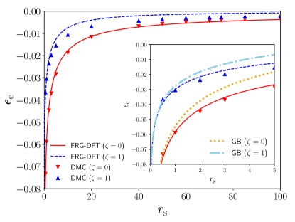
Figure 2: Correlation energy per particle $\epsilon_{\text{c}}$ for three-dimensional ($D=3$) homogeneous electron gas in the cases of $\zeta=0$ (paramagnetic) and $1$ (ferromagnetic) calculated by using the FRG-DFT (this work) and DMC shown as functions of Wigner-Seitz radius $r_{\text{s}}$. The data of DMC calculations are obtained from the values in Table IV in Ref. [39], which summarizes the results in Refs. [48, 50]. The inset is the enlarged view in $0\leq r_{\text{s}}\leq 5$, where the results by the GB resummation are also shown.

Table 1: Absolute difference $\Delta\epsilon_{\text{c}}=\left|\epsilon_{\text{c}}^{\text{FRG}}-\epsilon_{\text{c}}^{\text{DMC}}\right|$ and relative difference $\Delta\epsilon_{\text{c}}/\left|\epsilon_{\text{c}}^{\text{DMC}}\right|$ between the FRG-DFT result $\epsilon_{\text{c}}^{\text{FRG}}$ (this work) and DMC result $\epsilon_{\text{c}}^{\text{DMC}}$ [39] at $r_{\text{s}}=1$, $2$, $3$, $5$, $10$, $50$, and $100\,\mathrm{a.u.}$ and $\zeta=0$ and $1$.

	$r_{\text{s}}$ ($\mathrm{a.u.}$)	$1$	$2$	$3$	$5$	$10$	$50$	$100$
$\zeta=0$	$\Delta\epsilon_{\text{c}}\times 10^{4}$	$6.0$	$16.4$	$17.9$	$16.1$	$9.9$	$3.6$	$5.5$
	$\Delta\epsilon_{\text{c}}/|\epsilon_{\text{c}}^{\rm DMC}|$ ($\%$)	$1.0$	$3.7$	$4.8$	$5.7$	$5.3$	$6.2$	$17.0$
$\zeta=1$	$\Delta\epsilon_{\text{c}}\times 10^{4}$	$5.6$	$20.1$	$24.9$	$29.2$	$31.1$	$19.6$	$13.0$
	$\Delta\epsilon_{\text{c}}/\left|\epsilon_{\text{c}}^{\text{DMC}}\right|$ ($\%$)	$1.8$	$8.5$	$12.6$	$18.9$	$29.5$	$54.8$	$62.6$

In this section, we show the numerical results for HEG. Figure 2 shows the FRG-DFT results of $\epsilon_{\text{c},\,\lambda=1}$ in three dimensions in the paramagnetic ($\zeta=0$) and ferromagnetic ($\zeta=1$) states, together with the results by the diffusion Monte Carlo (DMC) simulation and the GB resummation, as functions of the Wigner-Seitz radius $r_{\text{s}}$.  The DMC results are obtained by subtracting the kinetic and exchange energies per particle from the total energy per particle given in Table IV in Ref. [39], which summarizes the results in Refs. [48, 50]. For both cases of $\zeta=0$ and $1$, the FRG-DFT reproduces the results by the GB resummation and the discrepancies between the FRG-DFT and DMC results decrease as $r_{\text{s}}$ becomes close to $0$, which is also indicated by the relative differences shown in Table 1. On the other hand, the increase of the relative differences at larger $r_{\text{s}}$ is due to the ignorance of the flow of the higher-order correlation functions as discussed in Sec. II.4. In the case of $\zeta=1$, FRG-DFT overestimates $\epsilon_{\text{c}}$ compared to DMC. This is a natural result since the truncation up to the second order breaks the Pauli-blocking condition [18, 19], which allows two electrons with the same spin to get closer to each other and increases the energy. At $\zeta=0$ and $r_{\text{s}}\gtrsim 40\,\mathrm{a.u.}$, FRG-DFT underestimates $\epsilon_{\text{c}}$ with smaller deviation compared to the case of $\zeta=1$ as indicated in the absolute and relative differences shown in Table 1. This suggests that the correlation between two electrons with the different spins is underestimated and compensates the overestimation coming from the correlation between those with the same spin.

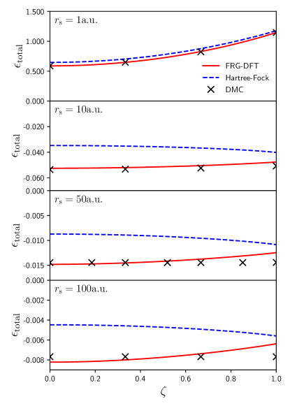
Figure 3: Total energy per particle $\epsilon_{\text{total}}$ at $r_{\text{s}}=1$, $10$, $50$, and $100\,\mathrm{a.u.}$ calculated by using the FRG-DFT shown as functions of $\zeta$. The results from the Hartree–Fock approximation and DMC are also shown. The data of DMC calculations are taken from Table IV in Ref. [39], which summarizes the results in Refs. [48, 50].

For the purpose to discuss stability of phases, we show the FRG-DFT results of the total energy per particle $\epsilon_{\text{total}}$ for arbitrary spin polarization at $r_{\text{s}}=1$, $10$, $50$, and $100\,\mathrm{a.u.}$ in Fig. 3. For comparison, this figure also shows the DMC results and the Hartree–Fock results. The latter are given by

$$\epsilon_{\text{total}}\left(r_{\text{s}},\zeta\right)\approx\epsilon_{\text{kin}}\left(r_{\text{s}},\zeta\right)+\epsilon_{\text{x},\,\lambda=1}\left(r_{\text{s}},\zeta\right),$$ (57)

where the kinetic term $\epsilon_{\text{kin}}$ and the exchange term $\epsilon_{\text{x}}$ are given by

$$\epsilon_{\text{kin}}\left(r_{\text{s}},\zeta\right)=\frac{3}{10}\left(\frac{9\pi}{4}\right)^{2/3}\frac{\left(1+\zeta\right)^{5/3}+\left(1-\zeta\right)^{5/3}}{2r_{\text{s}}^{2}},$$ (58)

and Eq. (23), respectively. According to the DMC results [48], a second order phase transition to spin-polarized states is found at $r_{\text{s}}=50\pm 2\,\mathrm{a.u.}$ and the system becomes (partially) spin-polarized states for larger $r_{\text{s}}$ and unpolarized one for smaller $r_{\text{s}}$. In contrast to this, the unpolarized state is stable even in $r_{\text{s}}\gtrsim 50\,\mathrm{a.u.}$ in the FRG-DFT result.

Next, we shall discuss the interpolation function $f_{\text{c}}\left(r_{\text{s}},\zeta\right)$ defined in Eq. (2). In Fig. 4(a), the results for $r_{\text{s}}=1$, $5$, $10$, $50$, and $100\,\mathrm{a.u.}$ calculated by using the FRG-DFT are shown as functions of $\zeta$. For comparison, DMC results and the interpolation function for the exchange part $f_{\text{x}}\left(\zeta\right)$ defined in Eq. (24) are also shown. Figure 4(b) shows the relative deviation of $f_{\text{c}}\left(r_{\text{s}},\zeta\right)$ from $f_{\text{x}}\left(\zeta\right)$: $\left[f_{\text{c}}\left(r_{\text{s}},\zeta\right)-f_{\text{x}}\left(\zeta\right)\right]/f_{\text{x}}\left(\zeta\right)$. A conventional approximation for $f_{\text{c}}\left(r_{\text{s}},\zeta\right)$ [Eq. (2)] is $f_{\text{c}}\left(r_{\text{s}},\zeta\right)\approx f_{\text{x}}\left(\zeta\right)$ [26, 24]. Actually, the DMC results in Fig. 4 suggest that this approximation is valid for $r_{\text{s}}\gtrsim 10\,\mathrm{a.u.}$ However, the FRG-DFT results show stronger $r_{\text{s}}$ dependence. Particularly, the deviation of the FRG-DFT results from $f_{\text{x}}\left(\zeta\right)$ can be seen in small $r_{\text{s}}$, where the FRG-DFT is accurate, as well as in large $r_{\text{s}}$. The deviation from $f_{\text{x}}\left(\zeta\right)$ also can be seen in the DMC results in $r_{\text{s}}\lesssim 5\,\mathrm{a.u.}$

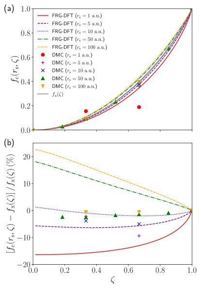
Figure 4: (a) Interpolation function $f_{\text{c}}\left(r_{\text{s}},\zeta\right)$ for $r_{\text{s}}=1$, $5$, $10$, $50$, and $100\,\mathrm{a.u.}$ calculated by using the FRG-DFT as functions of $\zeta$. For comparison, DMC results [48, 50] and $f_{\text{x}}\left(\zeta\right)$ [Eq. (24)] are also shown. (b) Relative deviation of $f_{\text{c}}\left(r_{\text{s}},\zeta\right)$ from $f_{\text{x}}\left(\zeta\right)$. The data at $\zeta=0$, where $f_{\text{x}}\left(\zeta\right)=0$, are excluded. The DMC data at $r_{\text{s}}=1\,\mathrm{a.u.}$ are out of the range of the figure.

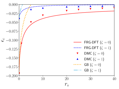
Figure 5: Correlation energy per particle $\epsilon_{\text{c}}$ at $\zeta=0$ and $1$ given by the FRG-DFT, DMC, and GB resummation in the two-dimensional ($D=2$) case. The data of DMC calculations are obtained from the values in Table VI in Ref. [39], which summarizes the results in Refs. [52, 53, 57]. The values at $r_{\text{s}}=0$ given by the FRG-DFT (and the GB resummation), which are finite in contrast to the three-dimensional case, are shown as the red and blue circles for $\zeta=0$ and $1$, respectively.

Finally, we mention the case of two dimensions. Figure 5 shows the FRG-DFT and DMC results of $r_{\text{s}}$ dependence of $\epsilon_{\text{c}}$ at $\zeta=0$ and $1$. The FRG-DFT result at $\zeta=0$ is the same as that in Ref. [22]. The DMC results are obtained from the total energies given in Refs. [52, 53, 57], which are summarized in Table VI in Ref. [39]. In dense cases, reproducing the exact results at $r_{\text{s}}=0\,\mathrm{a.u.}$ given by the GB resummation, the FRG-DFT results agree with the DMC results. On the other hand, the discrepancy between the FRG-DFT and DMC results increases as the system becomes dilute and the FRG-DFT respectively gives underestimated and overestimated results at $\zeta=0$ and $1$ in comparison with DMC. This behavior of $\epsilon_{\text{c}}$ favors the paramagnetic phase even if the system is dilute as in the case of three dimensions.

IV Conclusion

We have developed the functional-renormalization-group aided density functional theory (FRG-DFT) for the description of arbitrary spin-polarized systems and achieved numerical derivation of the correlation energy per particle of homogeneous electron gas $\epsilon_{\text{c}}$ with arbitrary density and spin polarization, which gives the energy density functional in the local spin density approximation. The hierarchical flow equations for the density correlation functions have been derived up to arbitrary order based on the FRG-DFT flow equation. Our numerical calculation has been performed based on the second order truncation for the hierarchical equations. Our correlation energy per particle reproduces the exact behavior at high-density limit given by the Gell-Mann–Brueckner resummation and agrees with the diffusion Monte Carlo (DMC) results in relatively high-density cases. On the other hand, the discrepancy between the FRG-DFT and DMC results becomes significant in the spin-polarized case in comparison with the spin-unpolarized case as the system becomes dilute. In contrast to DMC results, the correlation energy given by FRG-DFT stabilizes the spin-unpolarized state even in dilute cases. We also discuss the interpolation function $f_{\text{c}}\left(r_{\text{s}},\zeta\right)$, which characterizes the $\zeta$ dependence of $\epsilon_{\text{c}}$. We find the deviation from the interpolation function for the exchange part at small $r_{\text{s}}$, where the FRG-DFT gives accurate results.

The growth of the discrepancy in the spin-polarized case may be attributed to the effect of the Pauli blocking, which is broken in our approximation. In order to retain the Pauli-blocking effect, one may introduce a correction factor to the four-point density correlation function [18]. When applying this method, it is required to solve the flow equation numerically with respect to the evolution parameter $\lambda$. This is in contrast to the fact that the flow equation can be solved analytically in the approximation in this paper. The introduction of another approximation scheme valid even for dilute systems also may change the situation. In Ref. [63], a possibility of using small expansion parameters within some frameworks including the derivative expansion is discussed. As for the application of the derivative expansion in the framework of the functional renormalization group based on density, there is a work for classical liquids [64].

A great goal of studies of the FRG-DFT is systematic inclusion of the gradient effect. In dilute cases, particularly, this is important for the description of the Wigner crystal. One of the ways to realize this in our framework may be the use of the derivative expansion. Methods to describe solid-liquid phase transition developed for the classical DFT [65] are also expected to give hints for the treatment of the Wigner crystal.

Appendix A Derivation of Eqs. (15) and (16)

In this Appendix, we show the derivation of Eqs. (15) and (16). Equation (15) is derived from Eq. (13) and

$$\Gamma^{\text{({\hbox{ 2 }})}{-1}}_{\lambda,\,ss^{\prime}}\left[\rho_{\uparrow},\rho_{\downarrow}\right]\left(X,X^{\prime}\right)=G^{\text{({\hbox{ 2 }})}}_{\lambda,\,ss^{\prime}}\left(X,X^{\prime}\right).$$ (59)

The derivation of this relation is as follows: Differentiating Eq. (8), we have

$$\sum_{t}\int_{Y}\frac{\delta J_{\text{sup},\,\lambda,\,t}\left[\rho_{\uparrow},\rho_{\downarrow}\right]\left(Y\right)}{\delta\rho_{s^{\prime}}\left(X^{\prime}\right)}\frac{\delta^{2}W_{\lambda}\left[J_{\text{sup},\,\lambda,\,{\uparrow}}\left[\rho_{\uparrow},\rho_{\downarrow}\right],J_{\text{sup},\,\lambda,\,{\downarrow}}\left[\rho_{\uparrow},\rho_{\downarrow}\right]\right]}{\delta J_{t}\left(Y\right)\,\delta J_{s}\left(X\right)}=\delta_{ss^{\prime}}\delta\left(X-X^{\prime}\right).$$ (60)

By use of Eqs. (11) and (II.2), this is rewritten as

$$\sum_{t}\int_{Y}\frac{\delta^{2}\Gamma_{\lambda}\left[\rho_{\uparrow},\rho_{\downarrow}\right]}{\delta\rho_{s^{\prime}}\left(X^{\prime}\right)\,\delta\rho_{t}\left(Y\right)}G^{\text{({\hbox{ 2 }})}}_{\lambda,\,ts}\left(Y,X\right)=\delta_{ss^{\prime}}\delta\left(X-X^{\prime}\right),$$ (61)

which is equivalent to Eq. (59).

The following relation is useful for the derivation of Eq. (16):

$$\sum_{s}\int_{X}G^{\text{({\hbox{ 2 }})}}_{\lambda,\,s_{m+1}s}\left(X_{m+1},X\right)\frac{\delta}{\delta\rho_{s}\left(X\right)}G^{\text{({\hbox{ m }})}}_{\lambda,\,s_{1}\ldots s_{m}}\left(X_{1},\ldots,X_{m}\right)=G^{\text{({\hbox{ m + 1 }})}}_{\lambda,\,s_{1}\ldots s_{m+1}}\left(X_{1},\ldots,X_{m+1}\right).$$ (62)

This is obtained by differentiating Eqs. (11) and (II.2):

$$\frac{\delta}{\delta\rho_{s}\left(X\right)}G^{\text{($m$)}}_{\lambda,\,s_{1}\ldots s_{m}}\left(X_{1},\ldots,X_{m}\right)=\frac{\delta}{\delta\rho_{s}\left(X\right)}\frac{\delta^{m}W_{\lambda}\left[J_{\text{sup},\,\lambda,\,{\uparrow}}\left[\rho_{\uparrow},\rho_{\downarrow}\right],J_{\text{sup},\,\lambda,\,{\downarrow}}\left[\rho_{\uparrow},\rho_{\downarrow}\right]\right]}{\delta J_{s_{1}}\left(X_{1}\right)\,\cdots\,\delta J_{s_{m}}\left(X_{m}\right)}$$

$$=\sum_{s_{m+1}}\int_{X_{m+1}}\frac{\delta J_{\text{sup},\,\lambda,\,s_{m+1}}\left[\rho_{\uparrow},\rho_{\downarrow}\right]\left(X_{m+1}\right)}{\delta\rho_{s}\left(X\right)}\frac{\delta^{m+1}W_{\lambda}\left[J_{\text{sup},\,\lambda,\,{\uparrow}}\left[\rho_{\uparrow},\rho_{\downarrow}\right],J_{\text{sup},\,\lambda,\,{\downarrow}}\left[\rho_{\uparrow},\rho_{\downarrow}\right]\right]}{\delta J_{s_{1}}\left(X_{1}\right)\,\cdots\,\delta J_{s_{m}}\left(X_{m}\right)\,\delta J_{s_{m+1}}\left(X_{m+1}\right)}$$

$$=\sum_{s_{m+1}}\int_{X_{m+1}}\frac{\delta^{2}\Gamma_{\lambda}\left[\rho_{\uparrow},\rho_{\downarrow}\right]}{\delta\rho_{s}\left(X\right)\,\delta\rho_{s_{m+1}}\left(X_{m+1}\right)}G^{\text{($m+1$)}}_{\lambda,\,s_{1}\ldots s_{m+1}}\left(X_{1},\ldots,X_{m+1}\right).$$ (63)

Multiplying $\Gamma^{\text{($2$)}{-1}}_{\lambda}$ to both sides and using Eq. (59), we have Eq. (62).

The derivation of Eq. (16) is based on the mathematical induction. As a first step, we derive the equation for $m=1$. Differentiating Eq. (13), we have

$$\partial_{\lambda}\frac{\delta\Gamma_{\lambda}\left[\rho_{\uparrow},\rho_{\downarrow}\right]}{\delta\rho_{s_{1}}\left(X_{1}\right)}= \,\frac{1}{2}\iint_{X,\,X^{\prime}}U_{\text{2b}}\left(X-X^{\prime}\right)\left[\rho_{\Delta}\left(X\right)\delta\left(X^{\prime}-X_{1}\right)+\rho_{\Delta}\left(X^{\prime}\right)\delta\left(X-X_{1}\right)\right]$$

$$\,+\frac{1}{2}\iint_{X,\,X^{\prime}}U_{\text{2b}}\left(X-X^{\prime}\right)\left[\sum_{s,\,s^{\prime}}\frac{\delta G^{\text{($2$)}}_{\lambda,\,ss^{\prime}}\left(X_{\epsilon^{\prime}},X^{\prime}\right)}{\delta\rho_{s_{1}}\left(X_{1}\right)}-\delta\left(X-X_{1}\right)\delta\left(\bm{x}-\bm{x}^{\prime}\right)\right].$$ (64)

Multiplying $G^{\text{($2$)}}_{\lambda}$ and using Eqs. (62) and (11), we obtain

$$\sum_{s}\int_{X}G^{\text{($2$)}}_{\lambda,\,s_{1}s}\left(X_{1},X\right)\partial_{\lambda}J_{\text{sup},\,\lambda,\,s}\left[\rho_{\uparrow},\rho_{\downarrow}\right]\left(X\right)$$

$$= \,\frac{1}{2}\sum_{s}\iint_{X,\,X^{\prime}}U_{\text{2b}}\left(X-X^{\prime}\right)\left[\rho_{\Delta}\left(X\right)G^{\text{($2$)}}_{\lambda,\,ss_{1}}\left(X^{\prime},X_{1}\right)+\rho_{\Delta}\left(X^{\prime}\right)G^{\text{($2$)}}_{\lambda,\,ss_{1}}\left(X,X_{1}\right)\right]$$

$$\,+\frac{1}{2}\iint_{X,\,X^{\prime}}U_{\text{2b}}\left(X-X^{\prime}\right)\left[\sum_{s\,s^{\prime}}G^{\text{($3$)}}_{\lambda,\,ss^{\prime}s_{1}}\left(X_{\epsilon^{\prime}},X^{\prime},X_{1}\right)-\sum_{s}\delta\left(\bm{x}-\bm{x}^{\prime}\right)G^{\text{($2$)}}_{\lambda,\,ss_{1}}\left(X,X_{1}\right)\right].$$ (65)

Remembering $\partial_{\lambda}G^{\text{($1$)}}_{\lambda,\,s}\left(X_{1}\right)=\partial_{\lambda}\rho_{s}\left(X_{1}\right)=0$, one finds that Eq. (65) is equivalent to Eq. (16) in the case of $m=1$.

Next, we assume that Eq. (16) holds for $m=j$ and derive the equation for $m=j+1$. Differentiating Eq. (16) for $m=j$ with respect to the density, multiplying $G^{\text{($2$)}}_{\lambda}$, and using Eq. (62), we obtain

$$\sum_{s}\int_{X}G^{\text{($2$)}}_{\lambda s_{j+1}s}\left(X_{j+1},X\right)\partial_{\lambda}\frac{\delta}{\delta\rho_{s}\left(X\right)}G^{\text{($j$)}}_{\lambda,\,s_{1}\ldots s_{j}}\left(X_{1},\ldots X_{j}\right)$$

$$=\sum_{s\,s^{\prime}}\iint_{X,\,X^{\prime}}G^{\text{($j+1$)}}_{\lambda,\,ss_{1}\ldots s_{j}}\left(X,X_{1},\ldots X_{j}\right)G^{\text{($2$)}}_{\lambda,\,s_{j+1}s^{\prime}}\left(X_{j+1},X^{\prime}\right)\partial_{\lambda}\frac{\delta J_{\text{sup},\,\lambda,\,s}\left[\rho_{\uparrow},\rho_{\downarrow}\right]\left(X\right)}{\delta\rho_{s^{\prime}}\left(X^{\prime}\right)}$$

$$\quad+\sum_{s}\int_{X}G^{\text{($j+2$)}}_{\lambda,\,ss_{1}\ldots s_{j+1}}\left(X,X_{1},\ldots X_{j+1}\right)\partial_{\lambda}J_{\text{sup},\,\lambda,\,s}\left[\rho_{\uparrow},\rho_{\downarrow}\right]\left(X\right)$$

$$\quad-\frac{1}{2}\sum_{s\,s^{\prime}}\iint_{X,\,X^{\prime}}U_{\text{2b}}\left(X,X^{\prime}\right)$$

$$\qquad\times\left(G^{\text{($2$)}}_{\lambda,\,s^{\prime}s_{j+1}}\left(X,X_{j+1}\right)G^{\text{($j+1$)}}_{\lambda,\,ss_{1}\ldots s_{j}}\left(X^{\prime},X_{1},\ldots X_{j}\right)+G^{\text{($2$)}}_{\lambda,\,s^{\prime}s_{j+1}}\left(X^{\prime},X_{j+1}\right)G^{\text{($j+1$)}}_{\lambda,\,ss_{1}\ldots s_{j}}\left(X,X_{1},\ldots X_{j}\right)\right)$$

$$\quad-\frac{1}{2}\sum_{s}\iint_{X,\,X^{\prime}}U_{\text{2b}}\left(X,X^{\prime}\right)\left(\rho_{\Delta}\left(X\right)G^{\text{($j+2$)}}_{\lambda,\,ss_{1}\ldots s_{j+1}}\left(X^{\prime},X_{1},\ldots X_{j+1}\right)+\rho_{\Delta}\left(X^{\prime}\right)G^{\text{($j+2$)}}_{\lambda,\,ss_{1}\ldots s_{j+1}}\left(X,X_{1},\ldots X_{j+1}\right)\right)$$

$$\quad-\frac{1}{2}\sum_{s\,s^{\prime}}\iint_{X,\,X^{\prime}}U_{\text{2b}}\left(X,X^{\prime}\right)\left(G^{\text{($j+2$)}}_{\lambda,\,ss^{\prime}s_{1}\ldots s_{j+1}}\left(X_{\epsilon^{\prime}},X^{\prime},X_{1},\ldots X_{j+1}\right)-G^{\text{($j+2$)}}_{\lambda,\,ss_{1}\ldots s_{j+1}}\left(X,X_{1},\ldots X_{j+1}\right)\delta_{ss^{\prime}}\delta\left(\bm{x}-\bm{x}^{\prime}\right)\right.$$

$$\qquad\left.+\sum_{k=1}^{j-1}\frac{1}{k!\,\left(j-k\right)!}\sum_{\sigma\in S_{j}}\left.G^{\text{($k+2$)}}_{\lambda,\,ss_{\sigma\left(1\right)}\ldots s_{\sigma\left(k\right)}s_{j+1}}\left(X,X_{\sigma\left(1\right)},\ldots,X_{\sigma\left(k\right)},X_{j+1}\right)G^{\text{($j-k+1$)}}_{\lambda,\,s^{\prime}s_{\sigma\left(k+1\right)}\ldots s_{\sigma\left(j\right)}}\left(X^{\prime},X_{\sigma\left(k+1\right)},\ldots,X_{\sigma\left(j\right)}\right)\right.\right.$$

$$\qquad+\left.\left.G^{\text{($k+1$)}}_{\lambda,\,ss_{\sigma\left(1\right)}\ldots s_{\sigma\left(k\right)}}\left(X,X_{\sigma\left(1\right)},\ldots,X_{\sigma\left(k\right)}\right)G^{\text{($j-k+2$)}}_{\lambda,\,s^{\prime}s_{\sigma\left(k+1\right)}\ldots s_{\sigma\left(j\right)s_{j+1}}}\left(X^{\prime},X_{\sigma\left(k+1\right)},\ldots,X_{\sigma\left(j\right)},X_{j+1}\right)\right]\right).$$ (66)

The left-hand side is evaluated through the derivative of Eq. (62) with respect to $\lambda$:

$$\sum_{s}\int_{X}G^{\text{($2$)}}_{\lambda,\,s_{j+1}s}\left(X_{j+1},X\right)\partial_{\lambda}\frac{\delta}{\delta\rho_{s}\left(X\right)}G^{\text{($j$)}}_{\lambda,\,s_{1}\ldots s_{j}}\left(X_{1},\ldots,X_{j}\right)$$

$$=\partial_{\lambda}G^{\text{($j+1$)}}_{\lambda,\,s_{1}\ldots s_{j+1}}\left(X_{1},\ldots,X_{j+1}\right)\sum_{s}\int_{X}\partial_{\lambda}G^{\text{($2$)}}_{\lambda,\,s_{j+1}s}\left(X_{j+1},X\right)\frac{\delta}{\delta\rho_{s}\left(X\right)}G^{\text{($j$)}}_{\lambda,\,s_{1}\ldots s_{j}}\left(X_{1},\ldots,X_{j}\right).$$ (67)

By use of Eq. (60), this is rewritten as follows:

$$\sum_{s}\int_{X}G^{\text{($2$)}}_{\lambda,\,s_{j+1}s}\left(X_{j+1},X\right)\partial_{\lambda}\frac{\delta}{\delta\rho_{s}\left(X\right)}G^{\text{($j$)}}_{\lambda,\,s_{1}\ldots s_{j}}\left(X_{1},\ldots,X_{j}\right)$$

$$=\partial_{\lambda}G^{\text{($j+1$)}}_{\lambda,\,s_{1}\ldots s_{j+1}}\left(X_{1},\ldots,X_{j+1}\right)$$

$$\quad-\sum_{s\,s^{\prime}}\iint_{X,\,X^{\prime}}\partial_{\lambda}G^{\text{($2$)}}_{\lambda,\,s_{j+1}s}\left(X_{j+1},X\right)\sum_{t}\int_{Y}\frac{\delta J_{\text{sup},\,\lambda,\,t}\left[\rho_{\uparrow},\rho_{\downarrow}\right]\left(Y\right)}{\delta\rho_{s}\left(X\right)}G^{\text{($2$)}}_{\lambda,\,ts^{\prime}}\left(Y,X^{\prime}\right)\frac{\delta}{\delta\rho_{s^{\prime}}\left(X^{\prime}\right)}G^{\text{($j$)}}_{\lambda,\,s_{1}\ldots s_{j}}\left(X_{1},\ldots,X_{j}\right).$$ (68)

By differentiating Eq. (60) with respect to $\lambda$, we have

$$\sum_{s}\int_{X}\partial_{\lambda}G^{\text{({\hbox{ 2 }})}}_{\lambda,\,s_{j+1}s}\left(X_{j+1},X\right)\frac{\delta J_{\text{sup},\,\lambda,\,t}\left[\rho_{\uparrow},\rho_{\downarrow}\right]\left(Y\right)}{\delta\rho_{s}\left(X\right)}=-\sum_{s}\int_{X}G^{\text{({\hbox{ 2 }})}}_{\lambda,\,s_{j+1}s}\left(X_{j+1},X\right)\partial_{\lambda}\frac{\delta J_{\text{sup},\,\lambda,\,t}\left[\rho_{\uparrow},\rho_{\downarrow}\right]\left(Y\right)}{\delta\rho_{s}\left(X\right)}.$$ (69)

By use of this relation and Eq. (62), Eq. (68) is rewritten as follows:

$$\sum_{s}\int_{X}G^{\text{($2$)}}_{\lambda,\,s_{j+1}s}\left(X_{j+1},X\right)\partial_{\lambda}\frac{\delta}{\delta\rho_{s}\left(X\right)}G^{\text{($j$)}}_{\lambda,\,s_{1}\ldots s_{j}}\left(X_{1},\ldots,X_{j}\right)$$

$$=\partial_{\lambda}G^{\text{($j+1$)}}_{\lambda,\,s_{1}\ldots s_{j+1}}\left(X_{1},\ldots,X_{j+1}\right)+\sum_{s\,t}\iint_{X,\,Y}G^{\text{($j+1$)}}_{\lambda,\,ts_{1}\ldots s_{j}}\left(Y,X_{1},\ldots,X_{j}\right)G^{\text{($2$)}}_{\lambda,\,s_{j+1}s}\left(X_{j+1},X\right)\partial_{\lambda}\frac{\delta J_{\text{sup},\,\lambda,\,t}\left[\rho_{\uparrow},\rho_{\downarrow}\right]\left(Y\right)}{\delta\rho_{s}\left(X\right)}.$$ (70)

The second term of this equation and the first term in the right-hand side of Eq. (66) cancel each other. The last term in the right-hand side of Eq. (66) is deformed as follows:

$$\sum_{k=1}^{j-1}\frac{1}{k!\,\left(j-k\right)!}\sum_{\sigma\in S_{j}}\left[G^{\text{($k+2$)}}_{\lambda,\,ss_{\sigma\left(1\right)}\ldots\ldots s_{\sigma\left(k\right)}s_{j+1}}\left(X,X_{\sigma\left(1\right)},\ldots,X_{\sigma\left(k\right)},X_{j+1}\right)G^{\text{($j-k+1$)}}_{\lambda,\,s^{\prime}s_{\sigma\left(k+1\right)}\ldots\ldots s_{\sigma\left(j\right)}}\left(X^{\prime},X_{\sigma\left(k+1\right)},\ldots,X_{\sigma\left(j\right)}\right)\right.$$

$$\quad+\left.G^{\text{($k+1$)}}_{\lambda,\,ss_{\sigma\left(1\right)}\ldots\ldots s_{\sigma\left(k\right)}}\left(X,X_{\sigma\left(1\right)},\ldots,X_{\sigma\left(k\right)}\right)G^{\text{($j-k+2$)}}_{\lambda,\,s^{\prime}s_{\sigma\left(k+1\right)}\ldots\ldots s_{\sigma\left(j\right)}s_{j+1}}\left(X^{\prime},X_{\sigma\left(k+1\right)},\ldots,X_{\sigma\left(j\right)},X_{j+1}\right)\right]$$

$$=\sum_{\sigma\in S_{j}}\left[\sum_{k=2}^{j}\frac{1}{\left(k-1\right)!\,\left(j-k+1\right)!}G^{\text{($k+1$)}}_{\lambda,\,ss_{\sigma\left(1\right)}\ldots\ldots s_{\sigma\left(k-1\right)}s_{j+1}}\left(X,X_{\sigma\left(1\right)},\ldots,X_{\sigma\left(k-1\right)},X_{j+1}\right)G^{\text{($j-k+2$)}}_{\lambda,\,s^{\prime}s_{\sigma\left(k\right)}\ldots\ldots s_{\sigma\left(j\right)}}\left(X^{\prime},X_{\sigma\left(k\right)},\ldots,X_{\sigma\left(j\right)}\right)\right.$$

$$\quad\left.+\sum_{k=1}^{j-1}\frac{1}{k!\,\left(j-k\right)!}G^{\text{($k+1$)}}_{\lambda,\,ss_{\sigma\left(1\right)}\ldots\ldots s_{\sigma\left(k\right)}}\left(X,X_{\sigma\left(1\right)},\ldots,X_{\sigma\left(k\right)}\right)G^{\text{($j-k+2$)}}_{\lambda,\,s^{\prime}s_{\sigma\left(k+1\right)}\ldots\ldots s_{\sigma\left(j\right)}s_{j+1}}\left(X^{\prime},X_{\sigma\left(k+1\right)},\ldots,X_{\sigma\left(j\right)},X_{j+1}\right)\right]$$

$$=\sum_{\sigma\in S_{j}}\frac{1}{k!\,\left(j+1-k\right)!}\left[\sum_{k=2}^{j}kG^{\text{($k+1$)}}_{\lambda,\,ss_{\sigma\left(1\right)}\ldots\ldots s_{\sigma\left(k-1\right)}s_{j+1}}\left(X,X_{\sigma\left(1\right)},\ldots,X_{\sigma\left(k-1\right)},X_{j+1}\right)G^{\text{($j-k+2$)}}_{\lambda,\,s^{\prime}s_{\sigma\left(k\right)}\ldots\ldots s_{\sigma\left(j\right)}}\left(X^{\prime},X_{\sigma\left(k\right)},\ldots,X_{\sigma\left(j\right)}\right)\right.$$

$$\quad\left.+\sum_{k=1}^{j-1}\left(j+1-k\right)G^{\text{($k+1$)}}_{\lambda,\,ss_{\sigma\left(1\right)}\ldots\ldots s_{\sigma\left(k\right)}}\left(X,X_{\sigma\left(1\right)},\ldots,X_{\sigma\left(k\right)}\right)G^{\text{($j-k+2$)}}_{\lambda,\,s^{\prime}s_{\sigma\left(k+1\right)}\ldots\ldots s_{\sigma\left(j\right)}s_{j+1}}\left(X^{\prime},X_{\sigma\left(k+1\right)},\ldots,X_{\sigma\left(j\right)},X_{j+1}\right)\right]$$

$$=\sum_{\sigma\in S_{j}}\frac{1}{k!\,\left(j+1-k\right)!}\left[\sum_{k=1}^{j}kG^{\text{($k+1$)}}_{\lambda,\,ss_{\sigma\left(1\right)}\ldots\ldots s_{\sigma\left(k-1\right)}s_{j+1}}\left(X,X_{\sigma\left(1\right)},\ldots,X_{\sigma\left(k-1\right)},X_{j+1}\right)G^{\text{($j-k+2$)}}_{\lambda,\,s^{\prime}s_{\sigma\left(k\right)}\ldots\ldots s_{\sigma\left(j\right)}}\left(X^{\prime},X_{\sigma\left(k\right)},\ldots,X_{\sigma\left(j\right)}\right)\right.$$

$$\qquad\left.+\sum_{k=1}^{j-1}\left(j+1-k\right)G^{\text{($k+1$)}}_{\lambda,\,ss_{\sigma\left(1\right)}\ldots\ldots s_{\sigma\left(k\right)}}\left(X,X_{\sigma\left(1\right)},\ldots,X_{\sigma\left(k\right)}\right)G^{\text{($j-k+2$)}}_{\lambda,\,s^{\prime}s_{\sigma\left(k+1\right)}\ldots\ldots s_{\sigma\left(j\right)}s_{j+1}}\left(X^{\prime},X_{\sigma\left(k+1\right)},\ldots,X_{\sigma\left(j\right)},X_{j+1}\right)\right]$$

$$\quad-\sum_{\sigma\in S_{j}}\frac{1}{j!}\left[G^{\text{($2$)}}_{\lambda,\,ss_{j+1}}\left(X,X_{j+1}\right)G^{\text{($j+1$)}}_{\lambda,\,s^{\prime}s_{\sigma\left(1\right)}\ldots s_{\sigma\left(j\right)}}\left(X^{\prime},X_{\sigma\left(1\right)},\ldots,X_{\sigma\left(j\right)}\right)\right.$$

$$\qquad\left.+G^{\text{($j+1$)}}_{\lambda,\,ss_{\sigma\left(1\right)}\ldots s_{\sigma\left(j\right)}}\left(X,X_{\sigma\left(1\right)},\ldots,X_{\sigma\left(j\right)}\right)G^{\text{($2$)}}_{\lambda,\,s^{\prime}s_{j+1}}\left(X^{\prime},X_{j+1}\right)\right]$$

$$=\sum_{\sigma\in S_{j+1}}\sum_{k=1}^{j}\frac{1}{k!\,\left(j+1-k\right)!}G^{\text{($k+1$)}}_{\lambda,\,ss_{\sigma\left(1\right)}\ldots s_{\sigma\left(k\right)}}\left(X,X_{\sigma\left(1\right)},\ldots,X_{\sigma\left(k\right)}\right)G^{\text{($j-k+2$)}}_{\lambda,\,s^{\prime}s_{\sigma\left(k+1\right)}\ldots s_{\sigma\left(j+1\right)}}\left(X^{\prime},X_{\sigma\left(k+1\right)},\ldots,X_{\sigma\left(j+1\right)}\right)$$

$$\quad-G^{\text{($2$)}}_{\lambda,\,ss_{j+1}}\left(X,X_{j+1}\right)G^{\text{($j+1$)}}_{\lambda,\,s^{\prime}s_{1}\ldots s_{j}}\left(X^{\prime},X_{1},\ldots,X_{j}\right)-G^{\text{($j+1$)}}_{\lambda,\,ss_{1}\ldots s_{j}}\left(X,X_{1},\ldots,X_{j}\right)G^{\text{($2$)}}_{\lambda,\,s^{\prime}s_{j+1}}\left(X^{\prime},X_{j+1}\right).$$ (71)

By substituting Eqs. (70) and (71) into Eq. (66), we obtain Eq. (16) for $m=j+1$. Therefore, Eq. (16) holds for all integers $m\geq 1$.

References

• Hohenberg and Kohn [1964] P. Hohenberg and W. Kohn, Inhomogeneous Electron Gas, Phys. Rev. 136, B864 (1964).
• Kohn and Sham [1965] W. Kohn and L. J. Sham, Self-Consistent Equations Including Exchange and Correlation Effects, Phys. Rev. 140, A1133 (1965).
• Kohn [1999] W. Kohn, Nobel Lecture: Electronic structure of matter—wave functions and density functionals, Rev. Mod. Phys. 71, 1253 (1999).
• Perdew and Schmidt [2001] J. P. Perdew and K. Schmidt, Jacob’s ladder of density functional approximations for the exchange-correlation energy, AIP Conf. Proc. 577, 1 (2001).
• Fukuda et al. [1994] R. Fukuda, T. Kotani, Y. Suzuki, and S. Yokojima, Density Functional Theory through Legendre Transformation, Prog. Theor. Phys. 92, 833 (1994).
• Fukuda et al. [1995] R. Fukuda, M. Komachiya, S. Yokojima, Y. Suzuki, K. Okumura, and T. Inagaki, Novel use of Legendre transformation in field theory and many particle systems: On-shell expansion and inversion method, Prog. Theor. Phys. Suppl. 121, 1 (1995).
• Valiev and Fernando [1997] M. Valiev and G. W. Fernando, Generalized Kohn-Sham Density-Functional Theory via Effective Action Formalism, arXiv:cond-mat/9702247 (1997).
• Furnstahl [2020] R. J. Furnstahl, Turning the nuclear energy density functional method into a proper effective field theory: reflections, Eur. Phys. J. A 56, 85 (2020).
• Polonyi and Sailer [2002] J. Polonyi and K. Sailer, Effective actions and the density functional theory, Phys. Rev. B 66, 155113 (2002).
• Schwenk and Polonyi [2004] A. Schwenk and J. Polonyi, Towards density functional calculations from nuclear forces, in 32nd International Workshop on Gross Properties of Nuclei and Nuclear Excitation: Probing Nuclei and Nucleons with Electrons and Photons (Hirschegg 2004) Hirschegg, Austria, January 11-17, 2004 (2004) pp. 273–282, arXiv:nucl-th/0403011 .
• Wegner and Houghton [1973] F. J. Wegner and A. Houghton, Renormalization Group Equation for Critical Phenomena, Phys. Rev. A 8, 401 (1973).
• Wilson and Kogut [1974] K. G. Wilson and J. Kogut, The renormalization group and the $\epsilon$ expansion, Phys. Rep. 12, 75 (1974).
• Polchinski [1984] J. Polchinski, Renormalization and effective lagrangians, Nucl. Phys. B 231, 269 (1984).
• Wetterich [1993] C. Wetterich, Exact evolution equation for the effective potential, Phys. Lett. B 301, 90 (1993).
• Kemler and Braun [2013] S. Kemler and J. Braun, Towards a renormalization group approach to density functional theory–general formalism and case studies, J. Phys. G 40, 085105 (2013).
• Rentrop et al. [2015] J. F. Rentrop, S. G. Jakobs, and V. Meden, Two-particle irreducible functional renormalization group schemes—a comparative study, J. Phys. A 48, 145002 (2015).
• Liang et al. [2018] H. Liang, Y. Niu, and T. Hatsuda, Functional renormalization group and Kohn-Sham scheme in density functional theory, Phys. Lett. B 779, 436 (2018).
• Kemler et al. [2017] S. Kemler, M. Pospiech, and J. Braun, Formation of selfbound states in a one-dimensional nuclear model–a renormalization group based density functional study, J. Phys. G 44, 015101 (2017).
• Yokota et al. [2019a] T. Yokota, K. Yoshida, and T. Kunihiro, Functional renormalization-group calculation of the equation of state of one-dimensional uniform matter inspired by the Hohenberg-Kohn theorem, Phys. Rev. C 99, 024302 (2019a).
• Yokota et al. [2019b] T. Yokota, K. Yoshida, and T. Kunihiro, Ab initio description of excited states of 1D uniform matter with the Hohenberg–Kohn-theorem-inspired functional-renormalization-group method, Prog. Theor. Exp. Phys. 2019, 011D01 (2019b).
• Yokota et al. [2021] T. Yokota, J. Haruyama, and O. Sugino, Functional-renormalization-group approach to classical liquids with short-range repulsion: A scheme without repulsive reference system, Phys. Rev. E 104, 014124 (2021).
• Yokota and Naito [2019] T. Yokota and T. Naito, Functional-renormalization-group aided density functional analysis for the correlation energy of the two-dimensional homogeneous electron gas, Phys. Rev. B 99, 115106 (2019).
• Yokota and Naito [2021] T. Yokota and T. Naito, Ab initio construction of the energy density functional for electron systems with the functional-renormalization-group-aided density functional theory, Phys. Rev. Research 3, L012015 (2021).
• Martin [2004] R. M. Martin, Electronic Structure (Cambridge University Press, 2004).
• Jansen [1991] H. J. F. Jansen, Many-body properties calculated from the Kohn-Sham equations in density-functional theory, Phys. Rev. B 43, 12025 (1991).
• von Barth and Hedin [1972] U. von Barth and L. Hedin, A local exchange-correlation potential for the spin polarized case. I, J. Phys. C 5, 1629 (1972).
• Akmal et al. [1998] A. Akmal, V. R. Pandharipande, and D. G. Ravenhall, Equation of state of nucleon matter and neutron star structure, Phys. Rev. C 58, 1804 (1998).
• Dickhoff and Barbieri [2004] W. Dickhoff and C. Barbieri, Self-consistent Green’s function method for nuclei and nuclear matter, Prog. Part. Nucl. Phys. 52, 377 (2004).
• Stone and Reinhard [2007] J. R. Stone and P.-G. Reinhard, The Skyrme interaction in finite nuclei and nuclear matter, Prog. Part. Nucl. Phys. 58, 587 (2007).
• Gandolfi et al. [2010] S. Gandolfi, A. Y. Illarionov, S. Fantoni, J. C. Miller, F. Pederiva, and K. E. Schmidt, Microscopic calculation of the equation of state of nuclear matter and neutron star structure, Mon. Not. R. Astron. Soc. 404, L35 (2010).
• Lattimer [2012] J. M. Lattimer, The Nuclear Equation of State and Neutron Star Masses, Annu. Rev. Nucl. Part. Sci. 62, 485 (2012).
• Togashi and Takano [2013] H. Togashi and M. Takano, Variational study for the equation of state of asymmetric nuclear matter at finite temperatures, Nucl. Phys. A 902, 53 (2013).
• Togashi et al. [2016] H. Togashi, E. Hiyama, Y. Yamamoto, and M. Takano, Equation of state for neutron stars with hyperons using a variational method, Phys. Rev. C 93, 035808 (2016).
• Oertel et al. [2017] M. Oertel, M. Hempel, T. Klähn, and S. Typel, Equations of state for supernovae and compact stars, Rev. Mod. Phys. 89, 015007 (2017).
• Tong et al. [2018] H. Tong, X.-L. Ren, P. Ring, S.-H. Shen, S.-B. Wang, and J. Meng, Relativistic Brueckner-Hartree-Fock theory in nuclear matter without the average momentum approximation, Phys. Rev. C 98, 054302 (2018).
• Myo et al. [2019] T. Myo, H. Takemoto, M. Lyu, N. Wan, C. Xu, H. Toki, H. Horiuchi, T. Yamada, and K. Ikeda, Variational calculation of nuclear matter in a finite particle number approach using the unitary correlation operator and high-momentum pair methods, Phys. Rev. C 99, 024312 (2019).
• Wang et al. [2021] S. Wang, Q. Zhao, P. Ring, and J. Meng, Nuclear matter in relativistic Brueckner-Hartree-Fock theory with Bonn potential in the full Dirac space, Phys. Rev. C 103, 054319 (2021).
• Yokota et al. [2020] T. Yokota, H. Kasuya, K. Yoshida, and T. Kunihiro, Microscopic derivation of density functional theory for superfluid systems based on effective action formalism, Prog. Theor. Exp. Phys. 2021, 013A03 (2020).
• Loos and Gill [2016] P.-F. Loos and P. M. W. Gill, The uniform electron gas, WIREs Comput. Mol. Sci. 6, 410 (2016).
• Ceperley and Alder [1980] D. M. Ceperley and B. J. Alder, Ground State of the Electron Gas by a Stochastic Method, Phys. Rev. Lett. 45, 566 (1980).
• Vosko et al. [1980] S. H. Vosko, L. Wilk, and M. Nusair, Accurate spin-dependent electron liquid correlation energies for local spin density calculations: a critical analysis, Can. J. Phys. 58, 1200 (1980).
• Perdew and Zunger [1981] J. P. Perdew and A. Zunger, Self-interaction correction to density-functional approximations for many-electron systems, Phys. Rev. B 23, 5048 (1981).
• Ceperley [1978] D. Ceperley, Ground state of the fermion one-component plasma: A Monte Carlo study in two and three dimensions, Phys. Rev. B 18, 3126 (1978).
• Ortiz and Ballone [1994] G. Ortiz and P. Ballone, Correlation energy, structure factor, radial distribution function, and momentum distribution of the spin-polarized uniform electron gas, Phys. Rev. B 50, 1391 (1994).
• Ortiz and Ballone [1997] G. Ortiz and P. Ballone, Erratum: Correlation energy, structure factor, radial distribution function, and momentum distribution of the spin-polarized uniform electron gas [Phys. Rev. B 50, 1391 (1994)], Phys. Rev. B 56, 9970 (1997).
• Kwon et al. [1998] Y. Kwon, D. M. Ceperley, and R. M. Martin, Effects of backflow correlation in the three-dimensional electron gas: Quantum Monte Carlo study, Phys. Rev. B 58, 6800 (1998).
• Ortiz et al. [1999] G. Ortiz, M. Harris, and P. Ballone, Zero Temperature Phases of the Electron Gas, Phys. Rev. Lett. 82, 5317 (1999).
• Zong et al. [2002] F. H. Zong, C. Lin, and D. M. Ceperley, Spin polarization of the low-density three-dimensional electron gas, Phys. Rev. E 66, 036703 (2002).
• Drummond et al. [2004] N. D. Drummond, M. D. Towler, and R. J. Needs, Jastrow correlation factor for atoms, molecules, and solids, Phys. Rev. B 70, 235119 (2004).
• Spink et al. [2013] G. G. Spink, R. J. Needs, and N. D. Drummond, Quantum Monte Carlo study of the three-dimensional spin-polarized homogeneous electron gas, Phys. Rev. B 88, 085121 (2013).
• Tanatar and Ceperley [1989] B. Tanatar and D. M. Ceperley, Ground state of the two-dimensional electron gas, Phys. Rev. B 39, 5005 (1989).
• Kwon et al. [1993] Y. Kwon, D. M. Ceperley, and R. M. Martin, Effects of three-body and backflow correlations in the two-dimensional electron gas, Phys. Rev. B 48, 12037 (1993).
• Rapisarda and Senatore [1996] F. Rapisarda and G. Senatore, Diffusion Monte Carlo study of electrons in two-dimensional layers, Aust. J. Phys. 49, 161 (1996).
• Attaccalite et al. [2002] C. Attaccalite, S. Moroni, P. Gori-Giorgi, and G. B. Bachelet, Correlation Energy and Spin Polarization in the 2D Electron Gas, Phys. Rev. Lett. 88, 256601 (2002).
• Attaccalite et al. [2003] C. Attaccalite, S. Moroni, P. Gori-Giorgi, and G. B. Bachelet, Erratum: Correlation Energy and Spin Polarization in the 2D Electron Gas [Phys. Rev. Lett. 88, 256601 (2002)], Phys. Rev. Lett. 91, 109902 (2003).
• Gori-Giorgi et al. [2003] P. Gori-Giorgi, C. Attaccalite, S. Moroni, and G. B. Bachelet, Two-dimensional electron gas: Correlation energy versus density and spin polarization, Int. J. Quantum Chem. 91, 126 (2003).
• Drummond and Needs [2009] N. D. Drummond and R. J. Needs, Phase Diagram of the Low-Density Two-Dimensional Homogeneous Electron Gas, Phys. Rev. Lett. 102, 126402 (2009).
• Gell-Mann and Brueckner [1957] M. Gell-Mann and K. A. Brueckner, Correlation Energy of an Electron Gas at High Density, Phys. Rev. 106, 364 (1957).
• Rajagopal and Kimball [1977] A. K. Rajagopal and J. C. Kimball, Correlations in a two-dimensional electron system, Phys. Rev. B 15, 2819 (1977).
• Lewin et al. [2019] M. Lewin, E. H. Lieb, and R. Seiringer, The local density approximation in density functional theory, Pure Appl. Anal. 2, 35 (2019).
• Dirac [1930] P. A. M. Dirac, Note on Exchange Phenomena in the Thomas Atom, Math. Proc. Cambridge Philos. Soc. 26, 376–385 (1930).
• Friesecke [1997] G. Friesecke, Pair Correlations and Exchange Phenomena in the Free Electron Gas, Commun. Math. Phys. 184, 143 (1997).
• Dupuis et al. [2021] N. Dupuis, L. Canet, A. Eichhorn, W. Metzner, J. Pawlowski, M. Tissier, and N. Wschebor, The nonperturbative functional renormalization group and its applications, Phys. Rep. 910, 1 (2021).
• Lue [2015] L. Lue, Application of the functional renormalization group method to classical free energy models, AIChE Journal 61, 2985 (2015).
• Ramakrishnan and Yussouff [1979] T. V. Ramakrishnan and M. Yussouff, First-principles order-parameter theory of freezing, Phys. Rev. B 19, 2775 (1979).