Passive Mechanical Realizations of Bicubic Impedances with No More Than Five Elements for Inerter-Based Control Design

Abstract

This paper mainly investigates the passive realization problems of bicubic (third-order) impedances as damper-spring-inerter networks consisting of no more than five elements. First, the special case where a bicubic impedance contains a pole or a zero on the imaginary axis or at infinity is discussed. Then, assuming that there is no pole or zero on the imaginary axis or at infinity, the realizations of bicubic impedances as five-element networks are investigated. Necessary and sufficient conditions for the realizability as five-element series-parallel networks and as five-element non-series-parallel networks are derived, respectively, where 22 series-parallel configurations and 11 non-series-parallel configurations are presented to cover the conditions. Finally, two numerical examples together with positive-real controller designs for a quarter-car suspension system are presented for illustrations. The results of this paper can contribute to the synthesis of low-complexity passive mechanical (or electrical) networks, which are motivated by the synthesis and design of inerter-based vibration control systems.

Keywords: Passive network synthesis, bicubic positive-real impedances, five-element mechanical networks, inerter-based control

1 Introduction

As an important branch of system theory, passive network synthesis [1, 2, 3] is to realize passive systems, described by impedances, admittances, etc., as electrical (or mechanical) networks consisting of passive elements. Any network consisting of passive elements must be passive, and the impedance of any two-terminal linear time-invariant passive network is positive-real [1]. The impedance is defined as $Z(s):=V(s)/I(s)$, where $V(s)$ and $I(s)$ are Laplace transforms of port voltage and current, respectively, and a real-rational function $Z(s)$ is defined to be positive-real if $\Re(Z(s))\geq 0$ for $\Re(s)>0$ (see [1, 2]). By the Bott-Duffin synthesis procedure [4], any positive-real impedance is realizable as a two-terminal passive network consisting of resistors, inductors, and capacitors (RLC network). However, a large number of redundant elements are generated by the synthesis procedure in many cases. So far, the passive realizations of positive-real impedances using the least number of elements have been essential problems in the field of passive network synthesis, which remain unsolved even for low-order positive-real impedances.

The analogy between passive electrical and mechanical networks has been completed since the invention of inerters, where the resistors, inductors, capacitors, and transformers are analogous to the dampers, springs, inerters, and levers, respectively, through the force-current analogy [5]. For a two-terminal mechanical network, the impedance $Z(s)$ (resp. admittance $Y(s)$) is defined to be the ratio of the Laplace transform of the relative velocity (resp. force) to the Laplace transform of the force (resp. relative velocity). Therefore, passive network synthesis can be completely applied to designing passive mechanical circuits, and damper-spring-inerter networks realizing positive-real impedance (or admittance) controllers have been widely applied to a series of passive or semi-active vibration control systems, such as vibration isolation systems [6, 7, 8], vehicle suspension systems [9, 10, 12, 2, 3, 14], train suspension systems [15], building vibration systems [16, 17, 18], wind turbine towers [19], etc. The inerter-based control approach has low cost and high reliability, and introducing inerters can provide better system performances. Therefore, after designing a suitable positive-real impedance (or admittance) controller by optimizing the system performances, the positive-real function can be further realized as a passive mechanical network consisting of dampers, springs, and inerters, by utilizing the approach of passive network synthesis. Moreover, the realizability conditions in network synthesis can be applied to the optimization of control systems, in order to satisfy the network complexity constraint (see [9, 10, 14]). Therefore, it is practically essential to investigate the area of passive network synthesis, especially the minimal realizations of low-order impedances.

Moreover, passive network synthesis can be applied to many other fields, such as microwave antenna circuit design [20], self-assembling circuit design [21], supercapacitor model synthesis [22], acoustics simulation [23], biometric image processing [24], frequency control [25], positive-real and negative imaginary systems [26, 27], etc. In recent years, there have been a series of new results on passive network synthesis (see [2, 28, 29, 30, 31, 32, 33, 34, 35, 36, 37, 38, 39, 40, 41]). Specifically, Kalman has made an independent call for a renewed attempt in passive network synthesis as an important branch of system theory [42].

It is essential to investigate the passive damper-spring-inerter realization problems of low-order impedances using the least number of elements, due to the practical constraints on space, cost, weight, etc., for mechanical systems. Many existing works have focused on the realization problems of biquadratic (second-order) impedances [31, 33, 36]. Recently, some investigations on bicubic (third-order) impedances have been made [30, 32, 37, 41], where the bicubic impedance is more general and can provide better system performances in vibration control systems with respect to the biquadratic case (see [10, 14, 15]). The minimal realizations of some specific classes of bicubic positive-real impedances have been investigated in [30, 37, 41]. The realization results of a bicubic positive-real impedance as a series-parallel network consisting of three energy storage elements and a finite number of resistors (dampers) have been derived in [32]. Since a bicubic positive-real impedance is realizable with no more than 13 elements (resp. 12 elements) by the Bott-Duffin synthesis procedure (resp. Pantell’s modified Bott-Duffin procedure [2, Section 2.4]), it is necessary to obtain the realization results of bicubic impedances with no more than $k$ elements for $k=1,2,...,11$, in order to completely solve the minimal realizations of bicubic impedances. Moreover, the realization results including the realizability conditions and covering configurations can be applied to the optimization designs of third-order positive-real impedance controllers in inerter-based vibration systems, such that the third-order positive-real controller to be obtained can always be realized as a passive damper-spring-inerter network satisfying the required complexity.

This paper is concerned with the realization problem of bicubic impedances as damper-spring-inerter networks containing no more than five elements, which is a critical starting point of solving minimal realizations of bicubic impedances. First, the realization problems of the bicubic impedances containing a pole or zero on $j\mathbb{R}\cup\infty$ with no more than five elements are investigated in Section 4. It is shown that the realization results of the bicubic impedance containing a pole or zero at the origin $s=0$ or infinity $s=\infty$ can be referred to the existing results in [37], and any bicubic positive-real impedance containing a finite pole or zero on $j\mathbb{R}\setminus\{0\}$ is realizable as a series-parallel network containing three energy storage elements and no more than two dampers (Theorem 1). Then, under the assumption that there is no pole or zero on $j\mathbb{R}\cup\infty$, the main realization results of this paper are derived in Section 5, where it can be proved that the least number of elements for realizations is five. A necessary and sufficient condition is derived for the realizability of such a bicubic impedance as a five-element series-parallel network (Theorem 2), by obtaining 22 covering configurations classified into six quartets (Figs. 1–6) and investigating their realizability conditions. Furthermore, a necessary and sufficient condition is derived for such a bicubic impedance to be realizable as a five-element non-series-parallel network (Theorem 3), by obtaining 11 covering configurations classified into five quartets (Figs. 7–11) and investigating their realizability conditions. Finally, two numerical examples together with positive-real controller designs for a quarter-car suspension system are presented for illustrations in Section 6, where it is shown that the third-order positive-real controller realizable as a five-element network using the results of this paper can provide better ride comfort performances than the second-order positive-real controller $K(s)$ realizable as a series-parallel (resp. non-series-parallel) network containing no more than nine (resp. eight) elements.

The contributions of this paper are summarized as follows. Since the least number of elements to realize the bicubic impedance with positive coefficients is five, the methodology and realization results of this paper can provide the guidance on investigating the realizations of bicubic impedances as passive networks with higher complexity, in order to finally solve the minimal realization problems of positive-real bicubic impedances. The realizability conditions and the network element values in explicit forms are derived in this paper, which makes it more convenient to obtain the network realizations compared with the classical Bott-Duffin synthesis procedure. Moreover, the realization results in this paper can be utilized in the optimization design of positive-real controllers realizable as five-element damper-spring-inerter networks in many vibration systems. As illustrated in this paper, for the quarter-car suspension systems, the optimal positive-real controller in the bicubic form realizable as five-element networks can provide both lower physical complexity and better ride comfort performances than the optimal positive-real controller in the biquadratic form. The numerical examples also show that using the five-element realization results in this paper, the positive-real bicubic impedance satisfying the corresponding realizability conditions can be realized with much fewer elements than the Bott-Duffin realizations.

The networks in this paper are assumed to be two-terminal linear time-invariant passive damper-spring-inerter networks, whose element values are positive and finite. The realization results can be directly applied to those of electrical RLC networks based on the analogy between passive electrical and mechanical systems (see [5]). For the brevity of this paper, the detailed proofs of some results can be referred to the supplementary material [43].

2 Problem Formulation

A bicubic impedance $Z(s)$ is a real-rational impedance function whose McMillan degree is three, which is denoted as $\delta(Z(s))=3$. The general form of a bicubic impedance can be expressed as

$$Z(s)=\frac{a_{3}s^{3}+a_{2}s^{2}+a_{1}s+a_{0}}{d_{3}s^{3}+d_{2}s^{2}+d_{1}s+d_{0}}=:\frac{a(s)}{d(s)},$$ (1)

where $a_{i},d_{j}\geq 0$ for $i,j=0,1,2,3$, and there is no common factor between $a(s)$ and $d(s)$. A necessary and sufficient condition for a bicubic impedance to be positive-real has been presented in [28, Theorem 13], which is shown as follows.

Lemma 1

[28] Consider a third-degree impedance $Z(s)$ in the form of (1), where $\delta(Z(s))=3$ and $a_{i},d_{j}\geq 0$ for $i,j=0,1,2,3$. Then, $Z(s)$ is positive real, if and only if $(a_{1}+d_{1})(a_{2}+d_{2})\geq(a_{0}+d_{0})(a_{3}+d_{3})$, and one of the following conditions holds with $f_{0}:=a_{0}d_{0}$, $f_{1}:=a_{1}d_{1}-a_{0}d_{2}-a_{2}d_{0}$, $f_{2}:=a_{2}d_{2}-a_{1}d_{3}-a_{3}d_{1}$, and $f_{3}:=a_{3}d_{3}$:

(a) $f_{3}=0$, $f_{2}\geq 0$, $f_{0}\geq 0$, and $-f_{1}\leq 2\sqrt{f_{0}f_{2}}$;

(b) $f_{3}>0$, $f_{0}\geq 0$, and (b1) or (b2) holds: (b1) $f_{1}\geq 0$ and $-f_{2}\leq\sqrt{3f_{1}f_{3}}$; (b2) $f_{2}^{2}>3f_{1}f_{3}$ and $2f_{2}^{3}-9f_{1}f_{2}f_{3}+27f_{0}f_{3}^{2}\geq 2(f_{2}^{2}-3f_{1}f_{3})^{3/2}$.

By applying the Bott-Duffin synthesis procedure [4] (resp. Pantell’s modified Bott-Duffin procedure [2, Section 2.4]), any positive-real bicubic impedance $Z(s)$ in the form of (1) is realizable as a series-parallel (resp. non-series-parallel) damper-spring-inerter network containing no more than 13 elements (resp. 12 elements). To simplify the complexity of mechanical network realizations, it is essential to investigate the restricted-complexity realization problems of bicubic impedances as damper-spring-inerter networks.

This paper aims to derive necessary and sufficient conditions for a bicubic impedance $Z(s)$ in the form of (1) to be realizable as a damper-spring-inerter network containing no more than five elements, and to present the realization configurations to cover the conditions.

3 Notations and Preliminaries

This section will introduce the notations utilized in the remaining part of this paper.

Following the definition in [44, Definition 8.24], the Bezoutian matrix $\mathcal{B}(a,d)$ of two third-degree polynomials $a(s)$ and $d(s)$ in (1) is a real symmetric $3\times 3$ matrix whose entries $\mathcal{B}_{ij}$ for $i,j=1,2,3$ satisfy

$$\frac{a(z)d(w)-d(z)a(w)}{z-w}=\sum_{i=1}^{3}\sum_{j=1}^{3}\mathcal{B}_{ij}z^{i-1}w^{j-1}.$$

Then, the following notations are introduced as follows:

$$\begin{split}\mathcal{B}_{11}:=a_{1}d_{0}-a_{0}d_{1},~{}~{}\mathcal{B}_{12}:=a_{2}d_{0}-a_{0}d_{2},~{}~{}\mathcal{B}_{13}:=a_{3}d_{0}-a_{0}d_{3},\\ \mathcal{B}_{22}:=\mathcal{B}_{13}+a_{2}d_{1}-a_{1}d_{2},~{}~{}\mathcal{B}_{23}:=a_{3}d_{1}-a_{1}d_{3},~{}~{}\mathcal{B}_{33}:=a_{3}d_{2}-a_{2}d_{3}.\end{split}$$

Moreover, one denotes

$$\begin{split}\Delta_{1}:=a_{1}a_{2}-a_{0}a_{3},~{}~{}\Delta_{2}:=d_{1}d_{2}-d_{0}d_{3},~{}~{}\mathcal{M}_{11}:=a_{1}d_{0}+a_{0}d_{1},\\ \mathcal{M}_{33}:=a_{3}d_{2}+a_{2}d_{3},~{}~{}\mathcal{M}_{12}:=a_{2}d_{0}+a_{0}d_{2},~{}~{}\mathcal{M}_{23}:=a_{3}d_{1}+a_{1}d_{3},~{}~{}\mathcal{M}_{13}:=a_{3}d_{0}+a_{0}d_{3}.\end{split}$$

Consider any two-terminal damper-spring-inerter network $N$ whose two terminals are labeled as $a$ and $a^{\prime}$. A linear graph whose edges correspond to all the elements of $N$ is called the network graph [30], [2, pg. 28]. Then, let $\mathcal{P}(a,a^{\prime})$ denote the path [45, pg. 14] whose terminal vertices [45, pg. 14] are $a$ and $a^{\prime}$, and let $\mathcal{C}(a,a^{\prime})$ denote the cut-set [45, pg. 28] that separates the network graph into two connected subgraphs containing terminals $a$ and $a^{\prime}$, respectively. Furthermore, a path $\mathcal{P}(a,a^{\prime})$ whose all edges correspond to springs (resp. inerters) is denoted as $k$-$\mathcal{P}(a,a^{\prime})$ (resp. $b$-$\mathcal{P}(a,a^{\prime})$); a cut-set $\mathcal{C}(a,a^{\prime})$ whose all edges correspond to springs (resp. inerters) is denoted as $k$-$\mathcal{C}(a,a^{\prime})$ (resp. $b$-$\mathcal{C}(a,a^{\prime})$).

In addition to network graphs, any two-terminal damper-spring-inerter network $N$ can be also described by a one-terminal-pair labeled graph $\mathcal{N}$ (see [39], [45, pg. 14]), where each label designate a passive element regardless of the element value. The dampers, springs, and inerters are labeled as $c_{i}$, $k_{i}$, and $b_{i}$, respectively.

The notations of the maps acting on the labeled graph are as follows:

• $\text{GDu}:=$ Graph duality, which takes the graph into its dual (see [45, Definition 3-12]) without changing the labels.

• $\text{Inv}:=$ Inversion, which preserves the graph but interchanges the labels of springs $k_{i}$ and inerters $b_{i}$, that is, springs to inerters and inerters to springs, with their labels $k_{i}$ to $b_{i}$ and $b_{i}$ to $k_{i}$.

• $\text{Dual}:=$ Network duality of one-terminal-pair labeled graph $:=\text{GDu}\circ\text{Inv}=\text{Inv}\circ\text{GDu}$.

An example to illustrate GDu, Inv, and Dual can be referred to the four configurations in Fig. 2. Their one-terminal-pair labeled graphs can be denoted as $\mathcal{N}_{2a}$, $\mathcal{N}_{2b}$, $\mathcal{N}_{2c}$, and $\mathcal{N}_{2d}$, respectively, satisfying $\mathcal{N}_{2b}=\text{Dual}(\mathcal{N}_{2a})$, $\mathcal{N}_{2c}=\text{Inv}(\mathcal{N}_{2a})$, and $\mathcal{N}_{2d}=\text{GDu}(\mathcal{N}_{2a})$.

As shown in [2, Section 2.7], [39], $Z(s)$ is realizable as the impedance of a network whose one-terminal-pair labeled graph is $\mathcal{N}$, if and only if $Z(s^{-1})$ is realizable as the impedance of a network whose one-terminal-pair labeled graph is $\text{Inv}(\mathcal{N})$ (principle of frequency inversion), if and only if $Z(s^{-1})$ is realizable as the admittance of a network whose one-terminal-pair labeled graph is $\text{GDu}(\mathcal{N})$ (principle of frequency-inverse duality), if and only if $Z(s)$ is realizable as the admittance of a network whose one-terminal-pair labeled graph is $\text{Dual}(\mathcal{N})$ (principle of duality).

4 Impedances With Poles or Zeros on Imaginary Axis or at Infinity

4.1 Pole or Zero at Origin or Infinity

For the case when a bicubic impedance $Z(s)$ in the form (1), where $a_{i},d_{j}\geq 0$ for $i,j=0,1,2,3$, contains a zero at $s=0$ (origin), it is clear that $a_{0}=0$. Then, the realization results of $Z(s)$ with no more than five elements have been presented in [37].

Moreover, the realization results for the case when $Z(s)$ contains a zero at $s=\infty$ can be directly obtained through $a_{k}\leftrightarrow a_{3-k}$ and $d_{k}\leftrightarrow d_{3-k}$ for $k=0,1$ (the principle of frequency inversion [2, Section 2.7], [39]); the realization results for the case when $Z(s)$ contains a pole at $s=0$ can be directly obtained through $a_{k}\leftrightarrow d_{k}$ for $k=0,1,2,3$ (the principle of duality [2, Section 2.7], [39]); the realization results for the case when $Z(s)$ contains a pole at $s=\infty$ can be directly obtained through $a_{k}\leftrightarrow d_{3-k}$ for $k=0,1,2,3$ (the principle of frequency-inverse duality [2, Section 2.7], [39]).

4.2 Non-Zero Finite Pole or Zero on Imaginary Axis

Consider a bicubic impedance $Z(s)$ in the form of (1), where $a_{i},d_{j}\geq 0$ for $i,j=0,1,2,3$, and $\delta(Z(s))=3$. The following theorem (Theorem 1) presents the realization results for the case when $Z(s)$ contains a finite pole or zero on $j\mathbb{R}\setminus\{0\}$.

Theorem 1

Consider a bicubic positive-real impedance $Z(s)$ in the form of (1), where $a_{i},d_{j}\geq 0$ for $i,j=0,1,2,3$, and $\delta(Z(s))=3$. If $Z(s)$ contains a finite pole or zero on $j\mathbb{R}\setminus\{0\}$, then $Z(s)$ is realizable as a series-parallel network containing three energy storage elements and no more than two dampers.

Proof: Assuming that $Z(s)$ contains a finite pole on $j\mathbb{R}\setminus\{0\}$, the impedance can be expressed as

$$Z(s)=\frac{a_{3}s^{3}+a_{2}s^{2}+a_{1}s+a_{0}}{(s^{2}+\omega_{1}^{2})(d_{3}s+d_{0}/\omega_{1}^{2})},$$ (2)

where $\omega_{1}>0$. If $Z(s)$ is positive-real, then based on [2, pg. 13], it follows from (2) that

$$Z(s)=\frac{2K_{1}s}{s^{2}+\omega_{1}^{2}}+\frac{c_{1}s+c_{0}}{d_{3}s+d_{0}/\omega_{1}^{2}}=:Z_{1}(s)+Z_{2}(s),$$ (3)

where $K_{1}>0$, $c_{0}\geq 0$, and $c_{1}\geq 0$. It is clear that $Z_{1}(s)$ in (3) is realizable as the parallel connection of a spring and an inerter. Based on the results in [36], $Z_{2}(s)$ in (3) is realizable as a series-parallel subnetwork containing one energy storage element and no more than two dampers. Therefore, $Z(s)$ is realizable as a series-parallel network containing three energy storage elements and no more than two dampers. Together with the principle of duality ($a_{k}\leftrightarrow d_{k}$ for $k=0,1,2,3$), a similar discussion can be applied to the case when $Z(s)$ contains a finite zero on $j\mathbb{R}\setminus\{0\}$. $\blacksquare$

Remark 1

It can be derived that a bicubic impedance $Z(s)$ in the form of (1), where $a_{i},d_{j}>0$ for $i,j=0,1,2,3$, contains a finite pole (resp. zero) on $j\mathbb{R}\setminus\{0\}$ if and only if $\Delta_{2}=0$ (resp. $\Delta_{1}=0$).

5 Main Results

This section will investigate the realizations of a bicubic impedance $Z(s)$ in the form of (1) without any pole or zero on $j\mathbb{R}\cup\infty$. Then, it is implied that $a_{i},d_{j}>0$ for $i,j=0,1,2,3$.

5.1 Basic Lemmas

The following two lemmas (Lemmas 2 and 3) present the topological restrictions of the network realizations of bicubic impedances.

Lemma 2

[46, Theorem 2] Consider a bicubic impedance $Z(s)$ in the form of (1), where $a_{i},d_{j}>0$ for $i,j=0,1,2,3$, $\delta(Z(s))=3$, and there is not any pole or zero on $j\mathbb{R}\cup\infty$. Then, the network graph of any network realizing $Z(s)$ cannot contain any of $k$-$\mathcal{P}(a,a^{\prime})$, $b$-$\mathcal{P}(a,a^{\prime})$, $k$-$\mathcal{C}(a,a^{\prime})$, or $b$-$\mathcal{C}(a,a^{\prime})$.

Lemma 3

Consider a bicubic impedance $Z(s)$ in the form of (1), where $a_{i},d_{j}>0$ for $i,j=0,1,2,3$, $\delta(Z(s))=3$, and there is not any pole or zero on $j\mathbb{R}\cup\infty$. Then, $Z(s)$ cannot be realized as the series or parallel connection of a lossless subnetwork and a general passive subnetwork.

Proof: It can be verified that the impedance $Z(s)$ must contain at least one pole or zero on $j\mathbb{R}\cup\infty$ due to the lossless subnetwork, which contradicts the assumption. $\blacksquare$

The following lemma (Lemma 4) presents the least number of elements and energy storage elements needed to realize a bicubic impedance.

Lemma 4

Consider a bicubic impedance $Z(s)$ in the form of (1), where $a_{i},d_{j}>0$ for $i,j=0,1,2,3$, $\delta(Z(s))=3$, and there is not any pole or zero on $j\mathbb{R}\cup\infty$. Then, any network realizing $Z(s)$ must contain at least five elements, where the number of energy storage elements is at least three.

Proof: Since it is shown in [1, pg. 370] that the McMillan degree of a given impedance is equal to the least number of energy storage elements, any network realizing $Z(s)$ must contain at least three energy storage elements. It is clear that any non-series-parallel configuration must contain at least five elements. For any series-parallel realization of $Z(s)$, the network can be decomposed as a parallel or series connection of two series-parallel subnetworks. By Lemma 3, each of these two subnetworks must contain at least one damper, which implies that any series-parallel network realizing $Z(s)$ also contains at least five elements. $\blacksquare$

5.2 Realizations as Five-Element Series-Parallel Networks

In Lemma 4, it is shown that any five-element series-parallel network realizing a bicubic impedance (1) without any pole or zero on $j\mathbb{R}\cup\infty$ contains the least number of elements. This subsection will derive the realization results of $Z(s)$ as five-element series-parallel networks. The following Lemmas 5–11 will be utilized to prove Theorem 2.

Lemma 5

Consider a bicubic impedance $Z(s)$ in the form of (1), where $a_{i},d_{j}>0$ for $i,j=0,1,2,3$, $\delta(Z(s))=3$, and there is not any pole or zero on $j\mathbb{R}\cup\infty$. Then, $Z(s)$ is realizable as a five-element series-parallel network, if and only if $Z(s)$ is realizable as one of the configurations in Figs. 1–6.

Proof: See Appendix A for details, where Lemmas 2–4 are utilized in the proof. $\blacksquare$

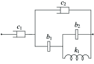
Figure 1: Five-element series-parallel configurations that can realize the bicubic impedance $Z(s)$ in (1), whose one-terminal-pair labeled graphs [39], [45, pg. 14] are (a) $\mathcal{N}_{1a}$ and (b) $\mathcal{N}_{1b}$, respectively, satisfying $\mathcal{N}_{1b}=\text{Dual}(\mathcal{N}_{1a})$. Moreover, the configurations whose one-terminal-pair labeled graphs are $\text{Inv}(\mathcal{N}_{1a})$ and $\text{GDu}(\mathcal{N}_{1a})$ can always be equivalent to the configurations in (b) and (a), respectively.

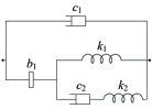
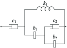
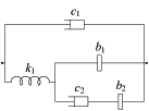
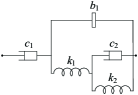
Figure 2: Five-element series-parallel configurations that can realize the bicubic impedance $Z(s)$ in (1), whose one-terminal-pair labeled graphs are (a) $\mathcal{N}_{2a}$, (b) $\mathcal{N}_{2b}$, (c) $\mathcal{N}_{2c}$, and (d) $\mathcal{N}_{2d}$, respectively, satisfying $\mathcal{N}_{2b}=\text{Dual}(\mathcal{N}_{2a})$, $\mathcal{N}_{2c}=\text{Inv}(\mathcal{N}_{2a})$, and $\mathcal{N}_{2d}=\text{GDu}(\mathcal{N}_{2a})$.

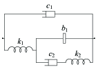
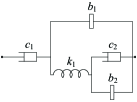
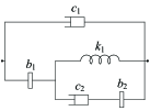
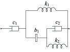
Figure 3: Five-element series-parallel configurations that can realize the bicubic impedance $Z(s)$ in (1), whose one-terminal-pair labeled graphs are (a) $\mathcal{N}_{3a}$, (b) $\mathcal{N}_{3b}$, (c) $\mathcal{N}_{3c}$, and (d) $\mathcal{N}_{3d}$, respectively, satisfying $\mathcal{N}_{3b}=\text{Dual}(\mathcal{N}_{3a})$, $\mathcal{N}_{3c}=\text{Inv}(\mathcal{N}_{3a})$, and $\mathcal{N}_{3d}=\text{GDu}(\mathcal{N}_{3a})$.

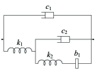
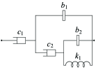
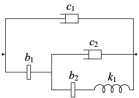
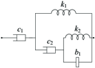
Figure 4: Five-element series-parallel configurations that can realize the bicubic impedance $Z(s)$ in (1), whose one-terminal-pair labeled graphs are (a) $\mathcal{N}_{4a}$, (b) $\mathcal{N}_{4b}$, (c) $\mathcal{N}_{4c}$, and (d) $\mathcal{N}_{4d}$, respectively, satisfying $\mathcal{N}_{4b}=\text{Dual}(\mathcal{N}_{4a})$, $\mathcal{N}_{4c}=\text{Inv}(\mathcal{N}_{4a})$, and $\mathcal{N}_{4d}=\text{GDu}(\mathcal{N}_{4a})$.

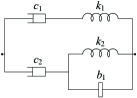
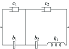
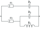
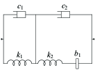
Figure 5: Five-element series-parallel configurations that can realize the bicubic impedance $Z(s)$ in (1), whose one-terminal-pair labeled graphs are (a) $\mathcal{N}_{5a}$, (b) $\mathcal{N}_{5b}$, (c) $\mathcal{N}_{5c}$, and (d) $\mathcal{N}_{5d}$, respectively, satisfying $\mathcal{N}_{5b}=\text{Dual}(\mathcal{N}_{5a})$, $\mathcal{N}_{5c}=\text{Inv}(\mathcal{N}_{5a})$, and $\mathcal{N}_{5d}=\text{GDu}(\mathcal{N}_{5a})$.

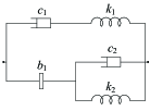
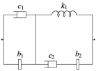
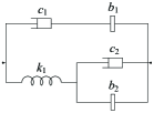
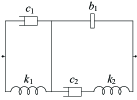
Figure 6: Five-element series-parallel configurations that can realize the bicubic impedance $Z(s)$ in (1), whose one-terminal-pair labeled graphs are (a) $\mathcal{N}_{6a}$, (b) $\mathcal{N}_{6b}$, (c) $\mathcal{N}_{6c}$, and (d) $\mathcal{N}_{6d}$, respectively, satisfying $\mathcal{N}_{6b}=\text{Dual}(\mathcal{N}_{6a})$, $\mathcal{N}_{6c}=\text{Inv}(\mathcal{N}_{6a})$, and $\mathcal{N}_{6d}=\text{GDu}(\mathcal{N}_{6a})$.

The above lemma (Lemma 5) presents a set of realization configurations in Figs. 1–6 that can cover all the cases of five-element series-parallel realizations. Then, the realizability conditions of these configurations need to be derived, which will be shown in the following Lemmas 6–11.

Lemma 6

Consider a bicubic impedance $Z(s)$ in the form of (1), where $a_{i},d_{j}>0$ for $i,j=0,1,2,3$, $\delta(Z(s))=3$, and there is not any pole or zero on $j\mathbb{R}\cup\infty$. Then, $Z(s)$ is realizable as one of the five-element series-parallel configurations in Fig. 1 (whose one-terminal-pair labeled graph is $\mathcal{N}_{1a}$ or $\mathcal{N}_{1b}$), if and only if $\mathcal{B}_{13}\neq 0$, $\mathcal{B}_{12}=0$, $\mathcal{B}_{23}=0$, and $\Delta_{1}>0$. Moreover, if $\mathcal{B}_{13}>0$, $\mathcal{B}_{12}=0$, $\mathcal{B}_{23}=0$, and $\Delta_{1}>0$, then $Z(s)$ is realizable as in Fig. 1 whose element values can be expressed as

$$\begin{split}c_{1}=\frac{d_{3}}{a_{3}},~{}~{}c_{2}=\frac{\mathcal{B}_{13}}{a_{0}a_{3}},~{}~{}k_{1}=\frac{d_{3}\mathcal{B}_{13}}{a_{3}^{2}d_{1}},~{}~{}k_{2}=\frac{\mathcal{B}_{13}\Delta_{1}}{a_{0}a_{1}a_{3}^{2}},~{}~{}b_{1}=\frac{\mathcal{B}_{13}\Delta_{1}}{a_{0}a_{1}^{2}a_{3}}.\end{split}$$ (4)

Proof: See Appendix B for details. $\blacksquare$

Lemma 7

Consider a bicubic impedance $Z(s)$ in the form of (1), where $a_{i},d_{j}>0$ for $i,j=0,1,2,3$, $\delta(Z(s))=3$, and there is not any pole or zero on $j\mathbb{R}\cup\infty$. Then, $Z(s)$ is realizable as one of the five-element series-parallel configurations in Fig. 2 (whose one-terminal-pair labeled graph is $\mathcal{N}_{2a}$, $\mathcal{N}_{2b}$, $\mathcal{N}_{2c}$, or $\mathcal{N}_{2d}$), if and only if one of the two conditions holds:

1. $\mathcal{B}_{13}=0$, $\Delta_{1}>0$, and either $a_{0}\mathcal{B}_{33}=a_{1}\mathcal{B}_{23}>0$ or $a_{3}\mathcal{B}_{11}=a_{2}\mathcal{B}_{12}<0$ holds;

2. $\mathcal{B}_{13}=0$, $\Delta_{2}>0$, and either $d_{0}\mathcal{B}_{33}=d_{1}\mathcal{B}_{23}<0$ or $d_{3}\mathcal{B}_{11}=d_{2}\mathcal{B}_{12}>0$ holds.

Moreover, if $\mathcal{B}_{13}=0$, $\Delta_{1}>0$, and $a_{0}\mathcal{B}_{33}=a_{1}\mathcal{B}_{23}>0$, then $Z(s)$ is realizable as in Fig. 2 whose element values can be expressed as

$$\begin{split}c_{1}=\frac{d_{3}}{a_{3}},~{}~{}c_{2}=\frac{\mathcal{B}_{33}\Delta_{1}}{a_{1}a_{2}^{2}a_{3}},~{}~{}k_{1}=\frac{d_{0}\mathcal{B}_{33}}{a_{1}a_{2}d_{3}},~{}~{}k_{2}=\frac{\mathcal{B}_{33}\Delta_{1}}{a_{1}a_{2}a_{3}^{2}},~{}~{}b_{1}=\frac{\mathcal{B}_{33}}{a_{1}a_{3}}.\end{split}$$ (5)

Proof: The method is similar to that of Lemma 6, which can be referred to [43, Section 2] for details. $\blacksquare$

Lemma 8

Consider a bicubic impedance $Z(s)$ in the form of (1), where $a_{i},d_{j}>0$ for $i,j=0,1,2,3$, $\delta(Z(s))=3$, and there is not any pole or zero on $j\mathbb{R}\cup\infty$. Then, $Z(s)$ is realizable as one of the five-element series-parallel configurations in Fig. 3 (whose one-terminal-pair labeled graph is $\mathcal{N}_{3a}$, $\mathcal{N}_{3b}$, $\mathcal{N}_{3c}$, or $\mathcal{N}_{3d}$), if and only if one of the following four conditions holds:

1. $\mathcal{B}_{33}\Delta_{1}=a_{2}a_{3}\mathcal{B}_{13}>0$ and $a_{2}\mathcal{B}_{33}=a_{3}\mathcal{B}_{23}>0$;

2. $\mathcal{B}_{33}\Delta_{2}=d_{2}d_{3}\mathcal{B}_{13}<0$ and $d_{2}\mathcal{B}_{33}=d_{3}\mathcal{B}_{23}<0$;

3. $\mathcal{B}_{11}\Delta_{1}=a_{0}a_{1}\mathcal{B}_{13}<0$ and $a_{1}\mathcal{B}_{11}=a_{0}\mathcal{B}_{12}<0$;

4. $\mathcal{B}_{11}\Delta_{2}=d_{0}d_{1}\mathcal{B}_{13}>0$ and $d_{1}\mathcal{B}_{11}=d_{0}\mathcal{B}_{12}>0$.

Moreover, if Condition 1 holds, then $Z(s)$ is realizable as the configuration in Fig. 3 whose element values can be expressed as

$$\begin{split}c_{1}=\frac{d_{3}}{a_{3}},~{}~{}c_{2}=\frac{\mathcal{B}_{13}}{a_{0}a_{3}},~{}~{}k_{1}=\frac{\mathcal{B}_{23}}{a_{2}a_{3}},~{}~{}k_{2}=\frac{a_{2}\mathcal{B}_{13}}{a_{0}a_{3}^{2}},~{}~{}b_{1}=\frac{\mathcal{B}_{23}}{a_{0}a_{3}}.\end{split}$$ (6)

Proof: The method is similar to that of Lemma 6, which can be referred to [43, Section 3] for details. $\blacksquare$

Lemma 9

Consider a bicubic impedance $Z(s)$ in the form of (1), where $a_{i},d_{j}>0$ for $i,j=0,1,2,3$, $\delta(Z(s))=3$, and there is not any pole or zero on $j\mathbb{R}\cup\infty$. Then, $Z(s)$ is realizable as one of the five-element series-parallel configurations in Fig. 4 (whose one-terminal-pair labeled graph is $\mathcal{N}_{4a}$, $\mathcal{N}_{4b}$, $\mathcal{N}_{4c}$, or $\mathcal{N}_{4d}$), if and only if one of the following four conditions holds:

1. $\mathcal{B}_{13}\Delta_{1}=a_{1}^{2}\mathcal{B}_{23}>0$ and $a_{1}\mathcal{B}_{33}=a_{3}\mathcal{B}_{13}>0$;

2. $\mathcal{B}_{13}\Delta_{2}=d_{1}^{2}\mathcal{B}_{23}<0$ and $d_{1}\mathcal{B}_{33}=d_{3}\mathcal{B}_{13}<0$;

3. $\mathcal{B}_{13}\Delta_{1}=a_{2}^{2}\mathcal{B}_{12}<0$ and $a_{2}\mathcal{B}_{11}=a_{0}\mathcal{B}_{13}<0$;

4. $\mathcal{B}_{13}\Delta_{2}=d_{2}^{2}\mathcal{B}_{12}>0$ and $d_{2}\mathcal{B}_{11}=d_{0}\mathcal{B}_{13}>0$.

Moreover, if Condition 1 holds, then $Z(s)$ is realizable as in Fig. 4 whose element values can be expressed as

$$\begin{split}c_{1}=\frac{d_{3}}{a_{3}},~{}~{}c_{2}=\frac{\mathcal{B}_{13}}{a_{0}a_{3}},~{}~{}k_{1}=\frac{\mathcal{B}_{13}}{a_{1}a_{3}},~{}~{}k_{2}=\frac{a_{1}\mathcal{B}_{23}}{a_{0}a_{3}^{2}},~{}~{}b_{1}=\frac{\mathcal{B}_{23}}{a_{0}a_{3}}.\end{split}$$ (7)

Proof: The method is similar to that of Lemma 6, which can be referred to [43, Section 4] for details. $\blacksquare$

Lemma 10

Consider a bicubic impedance $Z(s)$ in the form of (1), where $a_{i},d_{j}>0$ for $i,j=0,1,2,3$, $\delta(Z(s))=3$, and there is not any pole or zero on $j\mathbb{R}\cup\infty$. Then, $Z(s)$ is realizable as one of the five-element series-parallel configurations in Fig. 5 (whose one-terminal-pair labeled graph is $\mathcal{N}_{5a}$, $\mathcal{N}_{5b}$, $\mathcal{N}_{5c}$, or $\mathcal{N}_{5d}$), if and only if one of the following four conditions holds:

1. $a_{3}^{2}d_{0}^{2}\Delta_{2}=d_{2}^{2}\mathcal{B}_{12}\mathcal{B}_{13}>0$ and $a_{0}d_{2}^{2}\mathcal{B}_{12}=a_{3}d_{0}^{2}(a_{1}d_{2}-a_{3}d_{0})>0$;

2. $a_{0}^{2}d_{3}^{2}\Delta_{1}=a_{2}^{2}\mathcal{B}_{12}\mathcal{B}_{13}>0$ and $a_{2}^{2}d_{0}\mathcal{B}_{12}=a_{0}^{2}d_{3}(a_{0}d_{3}-a_{2}d_{1})<0$;

3. $a_{0}^{2}d_{3}^{2}\Delta_{2}=d_{1}^{2}\mathcal{B}_{23}\mathcal{B}_{13}>0$ and $a_{3}d_{1}^{2}\mathcal{B}_{23}=a_{0}d_{3}^{2}(a_{0}d_{3}-a_{2}d_{1})<0$;

4. $a_{3}^{2}d_{0}^{2}\Delta_{1}=a_{1}^{2}\mathcal{B}_{23}\mathcal{B}_{13}>0$ and $a_{1}^{2}d_{3}\mathcal{B}_{23}=a_{3}^{2}d_{0}(a_{1}d_{2}-a_{3}d_{0})>0$.

Moreover, if Condition 1 holds, then $Z(s)$ is realizable as the configuration in Fig. 5 whose element values can be expressed as

$$\begin{split}c_{1}=\frac{\mathcal{B}_{13}}{a_{0}a_{3}},~{}~{}c_{2}=\frac{d_{3}}{a_{3}},~{}~{}k_{1}=\frac{d_{2}\mathcal{B}_{13}}{a_{3}^{2}d_{0}},~{}~{}k_{2}=\frac{d_{2}d_{3}\mathcal{B}_{13}}{a_{3}^{2}\Delta_{2}},~{}~{}b_{1}=\frac{d_{2}^{2}d_{3}\mathcal{B}_{13}}{a_{3}^{2}d_{0}\Delta_{2}}.\end{split}$$ (8)

Proof: The method is similar to that of Lemma 6, which can be referred to [43, Section 5] for details. $\blacksquare$

Define the notation $\zeta_{1}$ as

$$\zeta_{1}:=\frac{a_{0}(\mathcal{B}_{23}\pm\sqrt{\mathcal{M}_{23}^{2}-4a_{0}a_{3}d_{2}d_{3}})}{2a_{3}}.$$ (9)

Then, the notations $\zeta_{2}$, $\zeta_{3}$, and $\zeta_{4}$ can be obtained from $\zeta_{1}$ according to the conversion $a_{k}\leftrightarrow d_{k}$ for $k=0,1,2,3$, the conversion $a_{k}\leftrightarrow a_{3-k}$ and $d_{k}\leftrightarrow d_{3-k}$ for $k=0,1$, and the conversion $a_{k}\leftrightarrow d_{3-k}$ for $k=0,1,2,3$, respectively. Then, the following lemma can be formulated.

Lemma 11

Consider a bicubic impedance $Z(s)$ in the form of (1), where $a_{i},d_{j}>0$ for $i,j=0,1,2,3$, $\delta(Z(s))=3$, and there is not any pole or zero on $j\mathbb{R}\cup\infty$. Then, $Z(s)$ is realizable as one of the five-element series-parallel configurations in Fig. 6 (whose one-terminal-pair labeled graph is $\mathcal{N}_{6a}$, $\mathcal{N}_{6b}$, $\mathcal{N}_{6c}$, or $\mathcal{N}_{6d}$), if and only if one of the following four conditions holds:

1. $0<\zeta_{1}<\min\{a_{1}d_{0},a_{0}d_{1}\}$, $\mathcal{M}_{23}^{2}-4a_{0}a_{3}d_{2}d_{3}\geq 0$, $a_{3}\zeta_{1}^{2}-a_{0}\mathcal{B}_{23}\zeta_{1}-a_{0}^{2}d_{3}(a_{1}d_{1}-a_{0}d_{2})=0$, and $\zeta_{1}^{3}-\mathcal{M}_{11}\zeta_{1}^{2}+a_{0}a_{1}d_{0}d_{1}\zeta_{1}-a_{0}^{3}d_{0}^{2}d_{3}=0$;

2. $0<\zeta_{2}<\min\{a_{1}d_{0},a_{0}d_{1}\}$, $\mathcal{M}_{23}^{2}-4a_{2}a_{3}d_{0}d_{3}\geq 0$, $d_{3}\zeta_{2}^{2}+d_{0}\mathcal{B}_{23}\zeta_{2}-a_{3}d_{0}^{2}(a_{1}d_{1}-a_{2}d_{0})=0$, and $\zeta_{2}^{3}-\mathcal{M}_{11}\zeta_{2}^{2}+a_{0}a_{1}d_{0}d_{1}\zeta_{2}-a_{0}^{2}a_{3}d_{0}^{3}=0$;

3. $0<\zeta_{3}<\min\{a_{3}d_{2},a_{2}d_{3}\}$, $\mathcal{M}_{12}^{2}-4a_{0}a_{3}d_{0}d_{1}\geq 0$, $a_{0}\zeta_{3}^{2}+a_{3}\mathcal{B}_{12}\zeta_{3}-a_{3}^{2}d_{0}(a_{2}d_{2}-a_{3}d_{1})=0$, and $\zeta_{3}^{3}-\mathcal{M}_{33}\zeta_{3}^{2}+a_{2}a_{3}d_{2}d_{3}\zeta_{3}-a_{3}^{3}d_{0}d_{3}^{2}=0$;

4. $0<\zeta_{4}<\min\{a_{3}d_{2},a_{2}d_{3}\}$, $\mathcal{M}_{12}^{2}-4a_{0}a_{1}d_{0}d_{3}\geq 0$, $d_{0}\zeta_{4}^{2}-d_{3}\mathcal{B}_{12}\zeta_{4}-a_{0}d_{3}^{2}(a_{2}d_{2}-a_{1}d_{3})=0$, and $\zeta_{4}^{3}-\mathcal{M}_{33}\zeta_{4}^{2}+a_{2}a_{3}d_{2}d_{3}\zeta_{4}-a_{0}a_{3}^{2}d_{3}^{3}=0$.

Moreover, if Condition 1 holds, then $Z(s)$ is realizable as the configuration in Fig. 6 whose element values can be expressed as

$$\begin{split}c_{1}=\frac{d_{0}}{a_{0}},~{}~{}c_{2}=\frac{d_{3}}{a_{3}},~{}~{}k_{1}=\frac{d_{0}^{2}}{a_{1}d_{0}-\zeta_{1}},~{}~{}k_{2}=\frac{a_{0}d_{0}d_{3}}{a_{3}\zeta_{1}},~{}~{}b_{1}=\frac{a_{0}d_{1}-\zeta_{1}}{a_{0}^{2}}.\end{split}$$ (10)

Proof: See Appendix C for details. $\blacksquare$

Then, combining Lemmas 5–11, the following Theorem 2 can be proved, which presents a necessary and sufficient condition for a bicubic impedance $Z(s)$ in the form of (1) to be realizable as a five-element series-parallel network.

Theorem 2

Consider a bicubic impedance $Z(s)$ in the form of (1), where $a_{i},d_{j}>0$ for $i,j=0,1,2,3$, $\delta(Z(s))=3$, and there is not any pole or zero on $j\mathbb{R}\cup\infty$. Then, $Z(s)$ is realizable as a five-element series-parallel network, if and only if one of the conditions in Lemmas 6–11 holds.

Proof: By Lemma 5, the bicubic impedance $Z(s)$ in this theorem is realizable as a five-element series-parallel network if and only if $Z(s)$ is realizable as one of the configurations in Figs. 1–6. Since the necessary and sufficient conditions for $Z(s)$ to be realizable as the configurations in Figs. 1–6 are shown in Lemmas 6–11, this theorem can be proved. $\blacksquare$

5.3 Realizations as Five-Element Non-Series-Parallel Networks

For the realizations as five-element non-series-parallel networks, the following Lemmas 12–17 will be utilized to prove Theorem 3.

Lemma 12

Consider a bicubic impedance $Z(s)$ in the form of (1), where $a_{i},d_{j}>0$ for $i,j=0,1,2,3$, $\delta(Z(s))=3$, and there is not any pole or zero on $j\mathbb{R}\cup\infty$. $Z(s)$ is realizable as a five-element non-series-parallel network, if and only if $Z(s)$ is realizable as one of the configurations in Figs. 7–11.

Proof: See Appendix D for details, where Lemmas 2 and 4 are utilized in the proof. $\blacksquare$

The above lemma (Lemma 12) presents a set of realization configurations in Figs. 7–11 that can cover all the cases of five-element non-series-parallel realizations. Then, the realizability conditions of these configurations need to be derived, which will be shown in the following Lemmas 13–17.

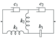
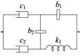
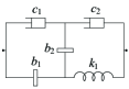
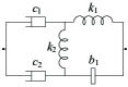
Figure 7: Five-element non-series-parallel configurations that can realize the bicubic impedance $Z(s)$ in (1), whose one-terminal-pair labeled graphs are (a) $\mathcal{N}_{7a}$, (b) $\mathcal{N}_{7b}$, (c) $\mathcal{N}_{7c}$, and (d) $\mathcal{N}_{7d}$, respectively, satisfying $\mathcal{N}_{7b}=\text{Dual}(\mathcal{N}_{7a})$, $\mathcal{N}_{7c}=\text{Inv}(\mathcal{N}_{7a})$, and $\mathcal{N}_{7d}=\text{GDu}(\mathcal{N}_{7a})$.

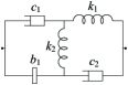
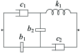
Figure 8: Five-element non-series-parallel configurations that can realize the bicubic impedance $Z(s)$ in (1), whose one-terminal-pair labeled graphs are (a) $\mathcal{N}_{8a}$ and (b) $\mathcal{N}_{8b}$, respectively, satisfying $\mathcal{N}_{8b}=\text{Dual}(\mathcal{N}_{8a})$, where $\text{Inv}(\mathcal{N}_{8a})=\text{Dual}(\mathcal{N}_{8a})$ and $\text{GDu}(\mathcal{N}_{8a})=\mathcal{N}_{8a}$.

Lemma 13

Consider a bicubic impedance $Z(s)$ in the form of (1), where $a_{i},d_{j}>0$ for $i,j=0,1,2,3$, $\delta(Z(s))=3$, and there is not any pole or zero on $j\mathbb{R}\cup\infty$. Then, $Z(s)$ is realizable as one of the five-element non-series-parallel configurations in Fig. 7 (whose one-terminal-pair labeled graph is $\mathcal{N}_{7a}$, $\mathcal{N}_{7b}$, $\mathcal{N}_{7c}$, or $\mathcal{N}_{7d}$), if and only if one of the following four conditions holds:

1. $\mathcal{B}_{13}>0$, $\mathcal{B}_{23}>0$, $\mathcal{B}_{13}(a_{2}d_{2}-\mathcal{B}_{23})-a_{2}^{2}d_{0}d_{3}=0$, and $\mathcal{B}_{13}\mathcal{B}_{23}\Delta_{1}-a_{2}^{2}a_{3}^{2}d_{0}^{2}=0$;

2. $\mathcal{B}_{13}<0$, $\mathcal{B}_{23}<0$, $\mathcal{B}_{13}(a_{2}d_{2}+\mathcal{B}_{23})+a_{0}a_{3}d_{2}^{2}=0$, and $\mathcal{B}_{13}\mathcal{B}_{23}\Delta_{2}-a_{0}^{2}d_{2}^{2}d_{3}^{2}=0$;

3. $\mathcal{B}_{13}<0$, $\mathcal{B}_{12}<0$, $\mathcal{B}_{13}(a_{1}d_{1}+\mathcal{B}_{12})+a_{1}^{2}d_{0}d_{3}=0$, and $\mathcal{B}_{13}\mathcal{B}_{12}\Delta_{1}-a_{0}^{2}a_{1}^{2}d_{3}^{2}=0$;

4. $\mathcal{B}_{13}>0$, $\mathcal{B}_{12}>0$, $\mathcal{B}_{13}(a_{1}d_{1}-\mathcal{B}_{12})-a_{0}a_{3}d_{1}^{2}=0$, and $\mathcal{B}_{13}\mathcal{B}_{12}\Delta_{2}-a_{3}^{2}d_{1}^{2}d_{0}^{2}=0$.

Moreover, if Condition 1 holds, then $Z(s)$ is realizable as the configuration in Fig. 7 whose element values can be expressed as

$$\begin{split}c_{1}=\frac{d_{0}d_{3}}{\mathcal{B}_{13}},~{}~{}c_{2}=\frac{d_{0}}{a_{0}},~{}~{}k_{1}=\frac{\mathcal{B}_{23}}{a_{2}a_{3}},~{}~{}k_{2}=\frac{a_{2}d_{0}^{2}}{a_{0}\mathcal{B}_{13}},~{}~{}b_{1}=\frac{a_{0}a_{3}}{\mathcal{B}_{23}}.\end{split}$$ (11)

Proof: The method is similar to that of Lemma 6, which can be referred to [43, Section 6] for details. $\blacksquare$

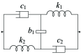
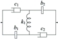
Figure 9: Five-element non-series-parallel configurations that can realize the bicubic impedance $Z(s)$ in (1), whose one-terminal-pair labeled graphs are (a) $\mathcal{N}_{9a}$ and (b) $\mathcal{N}_{9b}$, respectively, satisfying $\mathcal{N}_{9b}=\text{Dual}(\mathcal{N}_{9a})$, where $\text{Inv}(\mathcal{N}_{9a})=\text{Dual}(\mathcal{N}_{9a})$ and $\text{GDu}(\mathcal{N}_{9a})=\mathcal{N}_{9a}$.

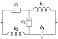
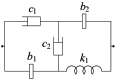
Figure 10: Five-element non-series-parallel configurations that can realize the bicubic impedance $Z(s)$ in (1), whose one-terminal-pair labeled graphs are (a) $\mathcal{N}_{10a}$ and (b) $\mathcal{N}_{10b}$, respectively, satisfying $\mathcal{N}_{10b}=\text{Dual}(\mathcal{N}_{10a})$, where $\text{Inv}(\mathcal{N}_{10a})=\text{Dual}(\mathcal{N}_{10a})$ and $\text{GDu}(\mathcal{N}_{10a})=\mathcal{N}_{10a}$.

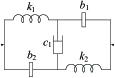
Figure 11: Five-element non-series-parallel configuration that can realize the bicubic impedance $Z(s)$ in (1), whose one-terminal-pair labeled graph is $\mathcal{N}_{11}$, where $\text{Dual}(\mathcal{N}_{11})=\text{Inv}(\mathcal{N}_{11})=\text{GDu}(\mathcal{N}_{11})=\mathcal{N}_{11}$.

Define the notations $\Lambda_{1a}$ and $\Lambda_{1b}$ as

$$\Lambda_{1a}:=\frac{d_{3}^{2}\mathcal{\mathcal{B}}_{11}}{\mathcal{B}_{13}\mathcal{M}_{13}},$$ (12)

and

$$\begin{split}\Lambda_{1b}:=\frac{1}{2a_{0}^{2}\mathcal{B}_{33}}\Bigg{(}\mathcal{B}_{13}\mathcal{M}_{13}-\mathcal{B}_{11}\mathcal{B}_{33}\pm\sqrt{(\mathcal{B}_{13}^{2}-\mathcal{B}_{11}\mathcal{B}_{33})(\mathcal{M}_{13}^{2}-\mathcal{B}_{11}\mathcal{B}_{33})}\Bigg{)}\end{split}$$ (13)

Then, the notation $\Lambda_{2a}$ and $\Lambda_{2b}$ can be respectively obtained from $\Lambda_{1a}$ and $\Lambda_{1b}$ according to the conversion $a_{k}\leftrightarrow d_{k}$ for $k=0,1,2,3$.

Lemma 14

Consider a bicubic impedance $Z(s)$ in the form of (1), where $a_{i},d_{j}>0$ for $i,j=0,1,2,3$, $\delta(Z(s))=3$, and there is not any pole or zero on $j\mathbb{R}\cup\infty$. Then, $Z(s)$ is realizable as one of the five-element non-series-parallel configurations in Fig. 8 (whose one-terminal-pair labeled graph is $\mathcal{N}_{8a}$ or $\mathcal{N}_{8b}$), if and only if one of the following four conditions holds:

1. $\mathcal{B}_{33}=0$, $\mathcal{B}_{11}\mathcal{B}_{13}>0$, $a_{0}^{2}a_{3}\Lambda_{1a}^{3}-a_{0}a_{3}d_{1}\Lambda_{1a}^{2}+a_{2}d_{0}d_{3}\Lambda_{1a}-d_{0}d_{3}^{2}=0$, and $a_{0}^{3}\mathcal{M}_{13}\Lambda_{1a}^{3}+a_{0}(2\mathcal{B}_{11}\mathcal{M}_{13}-a_{1}a_{3}d_{0}^{2})\Lambda_{1a}^{2}+\mathcal{B}_{11}(d_{3}\mathcal{B}_{11}-a_{3}d_{0}d_{1})\Lambda_{1a}+a_{3}d_{0}^{3}d_{3}=0$;

2. $\mathcal{B}_{33}\neq 0$, $(\mathcal{B}_{13}^{2}-\mathcal{B}_{11}\mathcal{B}_{33})(\mathcal{M}_{13}^{2}-\mathcal{B}_{11}\mathcal{B}_{33})\geq 0$, $a_{0}^{2}\Lambda_{1b}>\max\{0,-\mathcal{B}_{11}\}$, $a_{0}^{2}a_{3}\Lambda_{1b}^{3}-a_{0}a_{3}d_{1}\Lambda_{1b}^{2}+a_{2}d_{0}d_{3}\Lambda_{1b}-d_{0}d_{3}^{2}=0$, and $a_{0}^{3}\mathcal{M}_{13}\Lambda_{1b}^{3}+a_{0}(2\mathcal{B}_{11}\mathcal{M}_{13}-a_{1}a_{3}d_{0}^{2})\Lambda_{1b}^{2}+\mathcal{B}_{11}(d_{3}\mathcal{B}_{11}-a_{3}d_{0}d_{1})\Lambda_{1b}+a_{3}d_{0}^{3}d_{3}=0$;

3. $\mathcal{B}_{33}=0$, $\mathcal{B}_{11}\mathcal{B}_{13}>0$, $d_{0}^{2}d_{3}\Lambda_{2a}^{3}-a_{1}d_{0}d_{3}\Lambda_{2a}^{2}+a_{0}a_{3}d_{2}\Lambda_{2a}-a_{0}a_{3}^{2}=0$, and $d_{0}^{3}\mathcal{M}_{13}\Lambda_{2a}^{3}-d_{0}(2\mathcal{B}_{11}\mathcal{M}_{13}+a_{0}^{2}d_{1}d_{3})\Lambda_{2a}^{2}+\mathcal{B}_{11}(a_{3}\mathcal{B}_{11}+a_{0}a_{1}d_{3})\Lambda_{2a}+a_{0}^{3}a_{3}d_{3}=0$;

4. $\mathcal{B}_{33}\neq 0$, $(\mathcal{B}_{13}^{2}-\mathcal{B}_{11}\mathcal{B}_{33})(\mathcal{M}_{13}^{2}-\mathcal{B}_{11}\mathcal{B}_{33})\geq 0$, $d_{0}^{2}\Lambda_{2b}>\max\{0,\mathcal{B}_{11}\}$, $d_{0}^{2}d_{3}\Lambda_{2b}^{3}-a_{1}d_{0}d_{3}\Lambda_{2b}^{2}+a_{0}a_{3}d_{2}\Lambda_{2b}-a_{0}a_{3}^{2}=0$, and $d_{0}^{3}\mathcal{M}_{13}\Lambda_{2b}^{3}-d_{0}(2\mathcal{B}_{11}\mathcal{M}_{13}+a_{0}^{2}d_{1}d_{3})\Lambda_{2b}^{2}+\mathcal{B}_{11}(a_{3}\mathcal{B}_{11}+a_{0}a_{1}d_{3})\Lambda_{2b}+a_{0}^{3}a_{3}d_{3}=0$.

Moreover, if Condition 1 or 2 holds, then $Z(s)$ is realizable as the configuration in Fig. 8 whose element values can be expressed as

$$\begin{split}c_{1}=\frac{d_{0}}{a_{0}},~{}~{}c_{2}=\frac{d_{3}}{a_{3}},~{}~{}k_{1}=\frac{d_{0}^{2}}{a_{0}^{2}\gamma+\mathcal{B}_{11}},~{}~{}k_{2}=\frac{\gamma(a_{0}^{2}\gamma+\mathcal{B}_{11})}{a_{3}d_{0}},~{}~{}b_{1}=\gamma,\end{split}$$ (14)

where $\gamma=\Lambda_{1a}$ when Condition 1 holds and $\gamma=\Lambda_{1b}$ when Condition 2 holds.

Proof: See Appendix E for details. $\blacksquare$

Define the notations $\Gamma_{1}$, $\Phi_{1}$, and $\Psi_{1}$ as

$$\Gamma_{1}:=\frac{a_{3}d_{0}\pm\sqrt{a_{3}d_{0}(a_{3}d_{0}-4a_{0}d_{3})}}{2d_{0}d_{3}},$$ (15)

$$\begin{split}&\Phi_{1}:=\frac{1}{2a_{0}a_{3}d_{0}d_{2}\Gamma_{1}}\Bigg{(}a_{1}a_{3}d_{0}d_{2}\Gamma_{1}^{2}-(d_{0}^{2}d_{3}^{2}\Gamma_{1}^{4}-a_{0}^{2}a_{3}^{2})\\ &~{}~{}~{}~{}~{}\pm\sqrt{(a_{1}a_{3}d_{0}d_{2}\Gamma_{1}^{2}-(d_{0}d_{3}\Gamma_{1}^{2}-a_{0}a_{3})^{2})(a_{1}a_{3}d_{0}d_{2}\Gamma_{1}^{2}-(d_{0}d_{3}\Gamma_{1}^{2}+a_{0}a_{3})^{2})}\Bigg{)},\end{split}$$ (16)

and

$$\Psi_{1}:=\frac{a_{1}d_{2}+a_{3}d_{0}\pm\sqrt{(a_{1}d_{2}-a_{3}d_{0})^{2}-4a_{0}a_{3}d_{0}d_{3}}}{2d_{0}d_{2}}-\frac{d_{3}}{d_{2}}\Gamma_{1}.$$ (17)

Then, the notations $\Gamma_{2}$, $\Phi_{2}$, and $\Psi_{2}$ can be respectively obtained from $\Gamma_{1}$, $\Phi_{1}$, and $\Psi_{1}$ according to the conversion $a_{k}\leftrightarrow d_{k}$ for $k=0,1,2,3$.

Lemma 15

Consider a bicubic impedance $Z(s)$ in the form of (1), where $a_{i},d_{j}>0$ for $i,j=0,1,2,3$, $\delta(Z(s))=3$, and there is not any pole or zero on $j\mathbb{R}\cup\infty$. Then, $Z(s)$ is realizable as one of the five-element non-series-parallel configurations in Fig. 9 (whose one-terminal-pair labeled graph is $\mathcal{N}_{9a}$ or $\mathcal{N}_{9b}$), if and only if one of the following two conditions holds:

1. $0<\Phi_{1}/\Gamma_{1}<a_{1}/a_{0}$, $a_{3}d_{0}-4a_{0}d_{3}\geq 0$, $(a_{1}a_{3}d_{0}d_{2}\Gamma_{1}^{2}-(d_{0}d_{3}\Gamma_{1}^{2}-a_{0}a_{3})^{2})(a_{1}a_{3}d_{0}d_{2}\Gamma_{1}^{2}-(d_{0}d_{3}\Gamma_{1}^{2}+a_{0}a_{3})^{2})\geq 0$, $a_{0}(d_{0}d_{3}\Gamma_{1}^{2}-a_{0}a_{3})\Phi_{1}^{3}-(a_{1}d_{0}d_{3}\Gamma_{1}^{2}+a_{0}a_{3}d_{1}\Gamma_{1}-2a_{0}a_{1}a_{3})\Gamma_{1}\Phi_{1}^{2}+a_{1}a_{3}(d_{1}\Gamma_{1}-a_{1})\Gamma_{1}^{2}\Phi_{1}-a_{0}a_{3}d_{3}\Gamma_{1}^{4}=0$, and $a_{0}^{2}d_{0}\Phi_{1}^{4}-2a_{0}a_{1}d_{0}\Gamma_{1}\Phi_{1}^{3}+d_{0}(a_{1}^{2}+a_{0}a_{2})\Gamma_{1}^{2}\Phi_{1}^{2}+(a_{0}d_{0}d_{3}\Gamma_{1}^{2}-a_{1}a_{2}d_{0}\Gamma_{1}-a_{0}^{2}a_{3})\Gamma_{1}^{2}\Phi_{1}+a_{0}a_{1}a_{3}\Gamma_{1}^{3}=0$;

2. $0<\Phi_{2}/\Gamma_{2}<d_{1}/d_{0}$, $a_{0}d_{3}-4a_{3}d_{0}\geq 0$, $(a_{0}a_{2}d_{1}d_{3}\Gamma_{2}^{2}-(a_{0}a_{3}\Gamma_{2}^{2}-d_{0}d_{3})^{2})(a_{0}a_{2}d_{1}d_{3}\Gamma_{2}^{2}-(a_{0}a_{3}\Gamma_{2}^{2}+d_{0}d_{3})^{2})\geq 0$, $d_{0}(a_{0}a_{3}\Gamma_{2}^{2}-d_{0}d_{3})\Phi_{2}^{3}-(a_{0}a_{3}d_{1}\Gamma_{2}^{2}+a_{1}d_{0}d_{3}\Gamma_{2}-2d_{0}d_{1}d_{3})\Gamma_{2}\Phi_{2}^{2}+d_{1}d_{3}(a_{1}\Gamma_{2}-d_{1})\Gamma_{2}^{2}\Phi_{2}-a_{3}d_{0}d_{3}\Gamma_{2}^{4}=0$, and $a_{0}d_{0}^{2}\Phi_{2}^{4}-2a_{0}d_{0}d_{1}\Gamma_{2}\Phi_{2}^{3}+a_{0}(d_{1}^{2}+d_{0}d_{2})\Gamma_{2}^{2}\Phi_{2}^{2}+(a_{0}a_{3}d_{0}\Gamma_{2}^{2}-a_{0}d_{1}d_{2}\Gamma_{2}-d_{0}^{2}d_{3})\Gamma_{2}^{2}\Phi_{2}+d_{0}d_{1}d_{3}\Gamma_{2}^{3}=0$.

Moreover, if Condition 1 holds, then $Z(s)$ is realizable as the configuration in Fig. 9 whose element values can be expressed as

$$\begin{split}c_{1}=\Gamma_{1}^{-1},~{}c_{2}=\frac{d_{0}d_{3}\Gamma_{1}}{a_{0}a_{3}},~{}k_{1}=\Phi_{1}^{-1},~{}k_{2}=\frac{d_{0}d_{3}\Gamma_{1}^{2}}{a_{3}(a_{1}\Gamma_{1}-a_{0}\Phi_{1})},~{}b_{1}=\frac{d_{3}\Gamma_{1}^{2}}{(a_{1}\Gamma_{1}-a_{0}\Phi_{1})\Phi_{1}}.\end{split}$$ (18)

Proof: See Appendix F for details. $\blacksquare$

Lemma 16

Consider a bicubic impedance $Z(s)$ in the form of (1), where $a_{i},d_{j}>0$ for $i,j=0,1,2,3$, $\delta(Z(s))=3$, and there is not any pole or zero on $j\mathbb{R}\cup\infty$. Then, $Z(s)$ is realizable as one of the five-element non-series-parallel configurations in Fig. 10 (whose one-terminal-pair labeled graph is $\mathcal{N}_{10a}$ or $\mathcal{N}_{10b}$), if and only if one of the following two conditions holds:

1. $0<\Psi_{1}<a_{1}/d_{0}$, $a_{3}d_{0}-4a_{0}d_{3}\geq 0$, $(a_{1}d_{2}-a_{3}d_{0})^{2}-4a_{0}a_{3}d_{0}d_{3}\geq 0$, $d_{0}^{2}\Psi_{1}^{3}-a_{1}d_{0}\Psi_{1}^{2}+a_{2}d_{0}\Gamma_{1}\Psi_{1}-a_{0}a_{3}\Gamma_{1}=0$, and $d_{0}^{2}\Psi_{1}^{3}+d_{0}(d_{1}\Gamma_{1}-2a_{1})\Psi_{1}^{2}-a_{1}(d_{1}\Gamma_{1}-a_{1})\Psi_{1}+a_{0}d_{3}\Gamma_{1}^{2}=0$;

2. $0<\Psi_{2}<d_{1}/a_{0}$, $a_{0}d_{3}-4a_{3}d_{0}\geq 0$, $(a_{2}d_{1}-a_{0}d_{3})^{2}-4a_{0}a_{3}d_{0}d_{3}\geq 0$, $a_{0}^{2}\Psi_{2}^{3}-a_{0}d_{1}\Psi_{2}^{2}+a_{0}d_{2}\Gamma_{2}\Psi_{2}-d_{0}d_{3}\Gamma_{2}=0$, and $a_{0}^{2}\Psi_{2}^{3}+a_{0}(a_{1}\Gamma_{2}-2d_{1})\Psi_{2}^{2}-d_{1}(a_{1}\Gamma_{2}-d_{1})\Psi_{2}+a_{3}d_{0}\Gamma_{2}^{2}=0$.

Moreover, if Condition 1 holds, then $Z(s)$ is realizable as the configuration in Fig. 10 whose element values can be expressed as

$$\begin{split}c_{1}=\Gamma_{1}^{-1},~{}c_{2}=\frac{d_{0}d_{3}\Gamma_{1}}{a_{0}a_{3}},~{}k_{1}=\Psi_{1}^{-1},~{}k_{2}=\frac{d_{0}d_{3}\Gamma_{1}}{a_{3}(a_{1}-d_{0}\Psi_{1})},~{}b_{1}=\frac{d_{3}\Gamma_{1}}{(a_{1}-d_{0}\Psi_{1})\Psi_{1}}.\end{split}$$ (19)

Proof: The method is similar to that of Lemma 15, which can be referred to [43, Section 7] for details. $\blacksquare$

Lemma 17

Consider a bicubic impedance $Z(s)$ in the form of (1), where $a_{i},d_{j}>0$ for $i,j=0,1,2,3$, $\delta(Z(s))=3$, and there is not any pole or zero on $j\mathbb{R}\cup\infty$. Then, $Z(s)$ is realizable as the five-element non-series-parallel configuration in Fig. 11 (whose one-terminal-pair labeled graph is $\mathcal{N}_{11}$), if and only if $\mathcal{B}_{13}=0$, and there exists a positive root $T>0$ for the equation $a_{0}d_{0}d_{3}T^{3}+(a_{1}d_{0}d_{3}+a_{0}d_{1}d_{3}-a_{2}d_{0}d_{2})T^{2}+(a_{1}d_{1}d_{3}-a_{2}d_{0}d_{3}-a_{3}d_{0}d_{2})T-a_{3}d_{0}d_{3}=0$ such that $a_{0}d_{2}T^{2}+(a_{1}d_{2}-3a_{0}d_{3})T+a_{1}d_{3}\geq 0$, $(a_{2}^{2}d_{2}-4a_{0}a_{3}d_{3})T^{3}+(a_{2}^{2}d_{3}+2a_{2}a_{3}d_{2}-4a_{1}a_{3}d_{3})T^{2}+a_{3}(a_{3}d_{2}+2a_{2}d_{3})T+a_{3}^{2}d_{3}\geq 0$, $a_{1}T+a_{2}-a_{0}(y_{1}z_{1}+y_{2}z_{2})=0$, and $d_{1}T+d_{2}-d_{0}(y_{1}z_{2}+y_{2}z_{1})=0$, where $y_{1}$ and $y_{2}$ are two positive roots of the following equation in $y$:

$$d_{0}(d_{2}T+d_{3})y^{2}-(a_{0}T+a_{1})(d_{2}T+d_{3})y+a_{3}T(a_{0}T+a_{1})=0,$$ (20)

and $z_{1}$ and $z_{2}$ are two positive roots of the following equation in $z$:

$$a_{3}T(a_{0}T+a_{1})z^{2}-(a_{2}T+a_{3})(d_{2}T+d_{3})z+d_{3}T(d_{2}T+d_{3})=0.$$ (21)

Moreover, if the condition of this lemma holds, then $Z(s)$ is realizable as the configuration in Fig. 11, where

$$c_{1}=\frac{d_{3}}{a_{3}},~{}~{}k_{1}=y_{1}^{-1},~{}~{}k_{2}=y_{2}^{-1},~{}~{}b_{1}=z_{1},~{}~{}b_{2}=z_{2}.$$ (22)

Proof: See Appendix G for details. $\blacksquare$

Then, combining Lemmas 12–17, the following Theorem 3 can be proved, which presents a necessary and sufficient condition for a bicubic impedance $Z(s)$ in the form of (1) to be realizable as a five-element non-series-parallel network.

Theorem 3

Consider a bicubic impedance $Z(s)$ in the form of (1), where $a_{i},d_{j}>0$ for $i,j=0,1,2,3$, $\delta(Z(s))=3$, and there is not any pole or zero on $j\mathbb{R}\cup\infty$. Then, $Z(s)$ is realizable as a five-element non-series-parallel network, if and only if one of the conditions in Lemmas 13–17 holds.

Proof: By Lemma 12, the bicubic impedance $Z(s)$ in this theorem is realizable as a five-element non-series-parallel network if and only if $Z(s)$ is realizable as one of the configurations in Figs. 7–11. Since the necessary and sufficient conditions for $Z(s)$ to be realizable as the configurations in Figs. 7–11 are shown in Lemmas 13–17, this theorem can be proved. $\blacksquare$

6 Numerical Examples and Positive-Real Controller Designs for Inerter-Based Control Systems

In this section, two examples in the positive-real controller designs for a quarter-car suspension system will be presented for illustrations.

It is shown that the bicubic impedances satisfying the conditions of this paper (realizable with five elements) can provide better ride comfort performances compared with the biquadratic positive-real impedances (realizable with no more than nine elements by the Bott-Duffin procedure).

Consider a quarter-car suspension system as shown in Fig. 12, where the admittance $K(s)=1/Z(s)$ of a passive mechanical network can be regarded as the positive-real controller as shown in Fig. 12. Here, the spring with stiffness $k_{t}$ denotes the vehicle tyre, the sprung mass $m_{s}$ denotes the vehicle body, the unsprung mass $m_{u}$ denotes the vehicle wheel, $z_{s}$ denotes the displacement of the sprung mass, $z_{u}$ denotes the displacement of the unsprung mass, and $z_{r}$ denotes the road displacement.

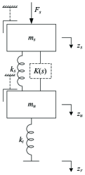
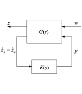
Figure 12: (a) A quarter-car vehicle suspension system model [2, 3], where the spring $k_{s}$ and the passive network whose admittance $K(s)=1/Z(s)$ constitute the suspension part. (b) Control synthesis diagram with positive-real controller $K(s)=1/Z(s)$.

As shown in [2], by Newton’s Second Law, the motion equations of the quarter-car suspension system in Fig. 12 can be formulated as

$$m_{s}\ddot{z}_{s}=F_{s}-F-k_{s}(z_{s}-z_{u}),~{}~{}~{}m_{u}\ddot{z}_{u}=F+k_{s}(z_{s}-z_{u})+k_{t}(z_{r}-z_{u}),$$ (23)

where $F$ is the output of the controller $K(s)$ satisfying $\hat{F}=K(s)(s\hat{z}_{s}-s\hat{z}_{u})$. Here, $\hat{F}$, $\hat{z}_{s}$, and $\hat{z}_{u}$ denote the Laplace transforms of $F$, $z_{s}$, and $z_{u}$, respectively. Furthermore, let $w=[F_{s},z_{r}]^{T}$ denote the input of the generalized plant, and let $z=[\dot{z}_{s},z_{s}]^{T}$ denote the performance output of the generalized plant. As a consequence, by letting the state vector satisfy $x=[\dot{z}_{s},z_{s},\dot{z}_{u},z_{u}]^{T}$, the motion equations in (23) can be written in the state-space form as follows:

$$\dot{x}=Ax+B\left[\begin{array}[]{c}w\\ F\\ \end{array}\right],~{}~{}~{}\left[\begin{array}[]{c}z\\ \dot{z}_{s}-\dot{z}_{u}\\ \end{array}\right]=Cx,$$ (24)

where

$$A=\left[\begin{array}[]{cccc}0&-\frac{k_{s}}{m_{s}}&0&\frac{k_{s}}{m_{s}}\\ 1&0&0&0\\ 0&\frac{k_{s}}{m_{u}}&0&-\frac{k_{s}+k_{t}}{m_{u}}\\ 0&0&1&0\\ \end{array}\right],~{}~{}B=\left[\begin{array}[]{ccc}\frac{1}{m_{s}}&0&-\frac{1}{m_{s}}\\ 0&0&0\\ 0&\frac{k_{t}}{m_{u}}&\frac{1}{m_{u}}\\ 0&0&0\\ \end{array}\right],~{}~{}C=\left[\begin{array}[]{cccc}1&0&0&0\\ 0&1&0&0\\ 1&0&-1&0\\ \end{array}\right].$$ (25)

Assume that $\{A_{k},B_{k},C_{k},D_{k}\}$ is a minimal realization of the positive-real controller $K(s)$, that is, $K(s)=C_{k}(sI-A_{k})^{-1}B_{k}+D_{k}$. Then,

$$\dot{x}_{k}=A_{k}x_{k}+B_{k}(\dot{z}_{s}-\dot{z}_{u}),~{}~{}~{}F=C_{k}x_{k}+D_{k}(\dot{z}_{s}-\dot{z}_{u}),$$ (26)

where the dimension of $x_{k}$ is equal to the McMillan degree of $K(s)$, which is denoted as $n_{k}$.

Assume that $F_{s}=0$. Then, combining (24)–(26), the closed-loop system whose input is $z_{r}$ and output is $\dot{z}_{s}$ can be obtained as

$$\dot{x}_{cl}=A_{cl}x_{cl}+B_{cl}z_{r},~{}~{}~{}\dot{z}_{s}=C_{cl}x_{cl},$$ (27)

where $x_{cl}=[x,x_{k}]^{T}$, and

$$A_{cl}=\left[\begin{array}[]{cc}A+B_{3}D_{k}C_{3}&B_{3}C_{k}\\ B_{k}C_{3}&A_{k}\\ \end{array}\right],~{}~{}~{}B_{cl}=\left[\begin{array}[]{c}B_{2}\\ \boldsymbol{0}_{n_{k}}\\ \end{array}\right],~{}~{}~{}C_{cl}=\left[\begin{array}[]{cc}C_{1}&\boldsymbol{0}_{n_{k}}^{T}\\ \end{array}\right].$$ (28)

Here, $B_{2}$ and $B_{3}$ denote the second and third columns of $B$, $C_{1}$ and $C_{3}$ denote the first and third rows of $C$, and $\boldsymbol{0}_{n_{k}}$ denotes the zero column vector whose dimension is $n_{k}$.

As shown in [3], the ride comfort index, which is the root-mean-square value of $\ddot{z}_{s}$, can be expressed as

$$J_{1}=2\pi\sqrt{V\kappa}\|s^{-1}T_{z_{r}\rightarrow\ddot{z}_{s}}\|_{2}=2\pi\sqrt{V\kappa}\|T_{z_{r}\rightarrow\dot{z}_{s}}\|_{2},$$ (29)

where $V$ denotes the vehicle speed, $\kappa$ denotes the road roughness parameter, and $T_{z_{r}\rightarrow\dot{z}_{s}}$ denotes the transfer function from $z_{r}$ to $\dot{z}_{s}$. The following lemma shown in [47, pg. 25] can be utilized to derive an equivalent form of $J_{1}$ in (29).

Lemma 18

[47, pg. 25] Consider a SISO closed-loop system (27). If $A_{cl}$ is stable, that is, $\Re(\lambda_{i}(A_{cl}))<0$, then the $H_{2}$ norm from the input $z_{r}$ to the output $\dot{z}_{s}$ satisfies

$$\|T_{z_{r}\rightarrow\dot{z}_{s}}\|_{2}^{2}=C_{cl}PC_{cl},$$

where the positive definite matrix $P>0$ is the unique solution of the Lyapunov equation

$$A_{cl}P+PA_{cl}^{T}=-B_{cl}B_{cl}^{T}.$$ (30)

Furthermore, assuming that $A_{cl}$ is stable, by Lemma 18, the ride comfort index $J_{1}$ as in (29) can be equivalent to

$$J_{1}=2\pi\sqrt{V\kappa}(C_{cl}PC_{cl})^{1/2},$$ (31)

where the positive definite matrix $P>0$ is the unique solution of the Lyapunov equation in (30). It is obvious that $P$ is related to $K(s)$. Therefore, the optimization problem of ride comfort $J_{1}$ is listed in the following procedure.

Procedure 1

Consider a quarter-car suspension system as in Fig. 12, whose motion equations satisfy the state-space form in (24). Assuming that $F_{s}=0$, the steps of designing a positive-real controller $K(s)$ to minimize the ride comfort performance $J_{1}$ in (29) (or (31)) for the closed-loop system in (27) are as follows.

1. Choose the McMillan degree $n$ of the positive-real controller $K(s)$, which is the admittance of a passive damper-spring-inerter network. Then, the impedance can be written as $Z(s):=1/K(s)=(a_{n}s^{n}+\cdots+a_{1}s+a_{0})/(d_{n}s^{n}+\cdots+d_{1}s+d_{0})$, where $a_{i},d_{j}\geq 0$ for $i,j=0,1,...,n$. Determine the positive-real condition and choose the further constraint conditions of the $n$th-order $Z(s)=1/K(s)$, which can guarantee $K(s)$ to be realizable as a specific class of passive damper-spring-inerter networks.

2. Calculate a minimal realization $\{A_{k},B_{k},C_{k},D_{k}\}$ of $K(s)$ satisfying (26), which is related to $a_{i},d_{j}$ for $i,j=0,1,...,n$.

3. Then, optimize the following problem:

   $$\begin{split}&\mathop{\min}_{a_{i},d_{j}}H_{1}:=C_{cl}PC_{cl},\\ &\text{s.t.}~{}~{}~{}A_{cl}~{}\text{is stable},~{}\\ &~{}~{}~{}~{}~{}~{}~{}P~{}\text{is the solution of \eqref{eq: lyp equation}},\\ &~{}~{}~{}~{}~{}~{}~{}Z(s)=1/K(s)~{}\text{is a class of positive-real impedances in Step~{}1},\end{split}$$

   where the optimization variables are the nonnegative coefficients $a_{i},d_{j}$ of $K(s)$, and the optimal positive-real controller can be obtained.

4. Calculate the optimal ride comfort performance by (31), that is, $J_{1}=2\pi\sqrt{V\kappa H_{1}}$.

5. Making use of the results of network synthesis, realize the positive-real controller $K(s)=1/Z(s)$ corresponding to the optimal performance as a damper-spring-inerter network.

For the case (Case A) when $Z(s)=1/K(s)$ is a bicubic (third-order) impedance as in (1), where $a_{i},d_{j}>0$ for $i,j=0,1,2,3$, one can further assume that $a_{i}$ and $d_{j}$ satisfy the conditions in Theorem 2 or 3. Then, the class of positive-real controllers in Step 1 of Procedure1 is chosen as above for this case. This means that any damper-spring-inerter realization of the optimal positive-real controller $K(s)=1/Z(s)$ contains no more than five elements, and the conditions in Lemmas 6–11 and 13–17 are regarded as the optimization constraints in Step 3 of Procedure 1.

For the case (Case B) when $Z(s)=1/K(s)$ is any biquadratic (second-order) positive-real impedance

$$Z(s)=\frac{a_{2}s^{2}+a_{1}s+a_{0}}{d_{2}s^{2}+d_{1}s+d_{0}},$$ (32)

where $a_{i},d_{j}>0$ for $i,j=0,1,2$ and $(\sqrt{a_{2}d_{0}}-\sqrt{a_{0}d_{2}})^{2}\leq a_{1}d_{1}$, any damper-spring-inerter realization of the optimal positive-real controller $K(s)=1/Z(s)$ contains no more than nine elements by using the Bott-Duffin procedure [4]. Then, the class of positive-real controllers in Step 1 of Procedure1 is chosen as above for this case.

Let the parameters of the suspension model satisfy $m_{s}=250$ kg, $m_{u}=35$ kg, $k_{t}=150$ kN/m, $V=25$ m/s, and $\kappa=5\times 10^{-7}$ m/cycle, which are the same as those in [3]. Following Procedure 1 where the optimization solver fmincon in MATLAB is utilized in Step 3, the optimal results of ride comfort $J_{1}$ for Case A (solid line) and Case B (dashed line) can be obtained as shown in Fig. 13, where the static stiffness $k_{s}$ is a fixed value ranging from $10$ kN/m to $120$ kN/m. It is shown that for different values of static stiffness $k_{s}$ the optimal performance values $J_{1}$ for Case A is enhanced compared with the values for Case B, and the percentage improvement can be over $9\%$ for small values of $k_{s}$. This means that the third-order positive-real controller $K(s)$ that is realizable as a five-element network using the results of this paper can provide better ride comfort performances than the second-order positive-real controller $K(s)$ that is realizable as a series-parallel (resp. non-series-parallel) network containing no more than nine (resp. eight) elements by using the Bott-Duffin procedure (resp. Pantell’s modified Bott-Duffin procedure). Therefore, the class of third-order positive-real controllers realizable as a five-element network can provide both lower physical complexity and better system performances than the conventional second-order positive-real controllers, which can also illustrate the significance of this paper.

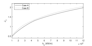
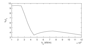
Figure 13: (a) The optimal performances $J_{1}$ for the case when $Z(s)=1/K(s)$ is any bicubic impedance satisfying the condition of Theorem 3 (Case A, solid line), and the case when $Z(s)=1/K(s)$ is any positive-real biquadratic impedance (Case B, dashed line), where the static stiffness $k_{s}$ ranges from $10$ kN/m to $120$ kN/m. (b) The percentage improvement of optimal performances for Case A and Case B, which is $(J_{1}^{(2)}-J_{1}^{(1)})/J_{1}^{(2)}\times 100\%$, where $J_{1}^{(1)}$ and $J_{1}^{(2)}$ are optimal performance values corresponding to Cases A and B, respectively.

The following two examples show the realization results of the positive-real controllers in the above optimization designs when the static stiffness $k_{s}$ satisfies $k_{s}=25$ kN/m and $k_{s}=70$ kN/m, respectively.

Example 1

When $k_{s}=25$ kN/m, the optimal value of $J_{1}$ for Case A satisfies $J_{1}^{(1)}=0.9182$, and the corresponding bicubic impedance $Z(s)$ is as in (1) with $a_{3}=5.994\times 10^{-4}$, $a_{2}=0.07188$, $a_{1}=1.529$, $a_{0}=14.818$, $d_{3}=1$, $d_{2}=5.005\times 10^{-8}$, $d_{1}=a_{1}d_{3}/a_{3}=2.55\times 10^{3}$, and $d_{0}=a_{0}d_{2}/a_{2}=1.031\times 10^{-5}$. Then, it can be checked that $\mathcal{B}_{13}=a_{3}d_{0}-a_{0}d_{3}=-14.818<0$, $\mathcal{B}_{12}=a_{2}d_{0}-a_{0}d_{2}=0$, $\mathcal{B}_{23}=a_{3}d_{1}-a_{1}d_{3}=0$, and $\Delta_{1}=a_{1}a_{2}-a_{0}a_{3}=0.10102>0$, which implies that the condition of Lemma 5 holds. Therefore, $Z(s)$ is realizable as the configuration in Fig. 1(b) with $c_{1}=1.668\times 10^{3}$ Ns/m, $c_{2}=6.96\times 10^{-7}$ Ns/m, $b_{1}=172.097$ kg, $b_{2}=15.131$ kg, and $k_{1}=3.858\times 10^{4}$ N/m, which is shown in Fig. 14. By the Bott-Duffin synthesis procedure, $Z(s)$ is realizable as the configuration in Fig. 14 with $c_{1}=6.956\times 10^{-7}$ Ns/m, $c_{2}=1.667\times 10^{3}$ Ns/m, $c_{3}=1.668\times 10^{3}$ Ns/m, $c_{4}=3.999\times 10^{12}$ Ns/m, $k_{1}=5.41\times 10^{8}$ N/m, $k_{2}=3.859\times 10^{4}$ N/m, $k_{3}=1.838\times 10^{5}$ N/m, $k_{4}=1.617\times 10^{4}$ N/m, $b_{1}=5.141\times 10^{-3}$ kg, $b_{2}=15.13$ kg, $b_{3}=72.066$ kg, and $b_{4}=172.028$ kg. For Case B, the optimal value of $J_{1}$ satisfies $J_{1}^{(2)}=1.0144$, and the corresponding biquadratic positive-real impedance $Z(s)$ is as in (32) with $a_{2}=1$, $a_{1}=226.559$, $a_{0}=1.34\times 10^{4}$, $d_{2}=5.083\times 10^{3}$, $d_{1}=7.6\times 10^{4}$, and $d_{0}=1.684\times 10^{7}$. By using the Bott-Duffin synthesis procedure, $Z(s)$ is realizable as a nine-element series-parallel configuration as the configuration in Fig. 14 with element values satisfying $c_{m}=5.476\times 10^{11}$ Ns/m, $c_{1}=1.257\times 10^{3}$ Ns/m, $c_{2}=5.083\times 10^{3}$ Ns/m, $k_{1}=5.664\times 10^{5}$ N/m, $k_{2}=6.564\times 10^{4}$ N/m, $k_{3}=6.487\times 10^{5}$ N/m, $b_{1}=11.28$ kg, $b_{2}=9.85$ kg, and $b_{3}=97.341$ kg.

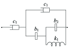
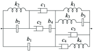
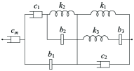
Figure 14: (a) A five-element network realization of the optimal bicubic impedance in Example 1, where the configuration is as in Fig. 1(b) and the element values satisfy $c_{1}=1.668\times 10^{3}$ Ns/m, $c_{2}=6.96\times 10^{-7}$ Ns/m, $b_{1}=172.097$ kg, $b_{2}=15.131$ kg, and $k_{1}=3.858\times 10^{4}$ N/m. (b) A Bott-Duffin realization of the optimal bicubic impedance in Example 1, where the element values satisfy $c_{1}=6.956\times 10^{-7}$ Ns/m, $c_{2}=1.667\times 10^{3}$ Ns/m, $c_{3}=1.668\times 10^{3}$ Ns/m, $c_{4}=3.999\times 10^{12}$ Ns/m, $k_{1}=5.41\times 10^{8}$ N/m, $k_{2}=3.859\times 10^{4}$ N/m, $k_{3}=1.838\times 10^{5}$ N/m, $k_{4}=1.617\times 10^{4}$ N/m, $b_{1}=5.141\times 10^{-3}$ kg, $b_{2}=15.13$ kg, $b_{3}=72.066$ kg, and $b_{4}=172.028$ kg. (c) A Bott-Duffin realization configuration of the optimal biquadratic positive-real impedance in Example 1, where the element values satisfy $c_{m}=5.476\times 10^{11}$ Ns/m, $c_{1}=1.257\times 10^{3}$ Ns/m, $c_{2}=5.083\times 10^{3}$ Ns/m, $k_{1}=5.664\times 10^{5}$ N/m, $k_{2}=6.564\times 10^{4}$ N/m, $k_{3}=6.487\times 10^{5}$ N/m, $b_{1}=11.28$ kg, $b_{2}=9.85$ kg, and $b_{3}=97.341$ kg.

Example 2

When $k_{s}=70$ kN/m, the optimal value of $J_{1}$ for Case A satisfies $J_{1}^{(1)}=1.579$, and the corresponding bicubic impedance $Z(s)$ is as in (1) with $a_{3}=279.553$, $a_{2}=4.239\times 10^{3}$, $a_{1}=2.398\times 10^{4}$, $a_{0}=2.232\times 10^{5}$, $d_{3}=1$, $d_{2}=9.3105$, $d_{1}=141.471$, and $d_{0}=798.595$. Then, it can be checked that the condition of Lemma 16 holds, where $T=0.1078$, $y_{1}=30.221$, $y_{2}=29.937$, $z_{1}=1.772\times 10^{-4}$, and $z_{2}=8.421\times 10^{-4}$. Therefore, $Z(s)$ is realizable as the configuration in Fig. 11 with $c_{1}=3.577\times 10^{-3}$ Ns/m, $k_{1}=0.03309$ N/m, $k_{2}=0.033403$ N/m, $b_{1}=1.772\times 10^{-4}$ kg, and $b_{2}=8.421\times 10^{-4}$ kg, which is shown in Fig. 15. By the Bott-Duffin synthesis procedure, $Z(s)$ is realizable as the configuration in Fig. 15 with $c_{1}=3.577\times 10^{-3}$ Ns/m, $c_{2}=1.261\times 10^{-5}$ Ns/m, $c_{3}=3.577\times 10^{-3}$ Ns/m, $c_{4}=1.261\times 10^{-5}$ Ns/m, $k_{1}=0.03367$ N/m, $k_{2}=0.02124$ N/m, $k_{3}=0.05203$ N/m, $k_{4}=1.168\times 10^{-4}$ N/m, $b_{1}=3.813\times 10^{-4}$ kg, $b_{2}=2.468\times 10^{-4}$ kg, $b_{3}=6.045\times 10^{-4}$ kg, and $b_{4}=1.357\times 10^{-6}$ kg. For Case B, the optimal value of $J_{1}$ satisfies $J_{1}^{(2)}=1.6498$, and the corresponding biquadratic positive-real impedance $Z(s)$ is as in (32) with $a_{2}=1$, $a_{1}=11.057$, $a_{0}=109.731$, $d_{2}=2.942\times 10^{3}$, $d_{1}=1.798\times 10^{4}$, and $d_{0}=1.496\times 10^{4}$. By using the Bott-Duffin synthesis procedure, $Z(s)$ is realizable as a nine-element series-parallel configuration in Fig. 15 with element values satisfying $c_{m}=3.537\times 10^{12}$ Ns/m, $c_{1}=136.323$ Ns/m, $c_{2}=2.942\times 10^{3}$ Ns/m, $k_{1}=1.921\times 10^{3}$ N/m, $k_{2}=379.207$ N/m, $k_{3}=2.498\times 10^{4}$ N/m, $b_{1}=208.8002$ kg, $b_{2}=16.054$ kg, and $b_{3}=1.058\times 10^{3}$ kg.

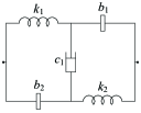
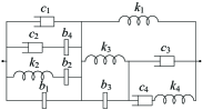
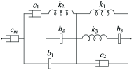
Figure 15: (a) A five-element network realization of the optimal bicubic impedance in Example 2, where the configuration is as in Fig. 11 and the element values satisfy $c_{1}=3.577\times 10^{-3}$ Ns/m, $k_{1}=0.03309$ N/m, $k_{2}=0.033403$ N/m, $b_{1}=1.772\times 10^{-4}$ kg, and $b_{2}=8.421\times 10^{-4}$ kg. (b) A Bott-Duffin realization of the optimal bicubic impedance in Example 2, where the element values satisfy $c_{1}=3.577\times 10^{-3}$ Ns/m, $c_{2}=1.261\times 10^{-5}$ Ns/m, $c_{3}=3.577\times 10^{-3}$ Ns/m, $c_{4}=1.261\times 10^{-5}$ Ns/m, $k_{1}=0.03367$ N/m, $k_{2}=0.02124$ N/m, $k_{3}=0.05203$ N/m, $k_{4}=1.168\times 10^{-4}$ N/m, $b_{1}=3.813\times 10^{-4}$ kg, $b_{2}=2.468\times 10^{-4}$ kg, $b_{3}=6.045\times 10^{-4}$ kg, and $b_{4}=1.357\times 10^{-6}$ kg. (c) A Bott-Duffin realization configuration of the optimal biquadratic positive-real impedance in Example 2, where the element values satisfy $c_{m}=3.537\times 10^{12}$ Ns/m, $c_{1}=136.323$ Ns/m, $c_{2}=2.942\times 10^{3}$ Ns/m, $k_{1}=1.921\times 10^{3}$ N/m, $k_{2}=379.207$ N/m, $k_{3}=2.498\times 10^{4}$ N/m, $b_{1}=208.8002$ kg, $b_{2}=16.054$ kg, and $b_{3}=1.058\times 10^{3}$ kg.

As shown in Examples 1 and 2, the five-element realization results derived in this paper can provide much fewer elements than the Bott-Duffin synthesis procedure, provided that the bicubic impedance satisfies the corresponding realizability conditions. Moreover, the five-element realizations can even contain fewer elements than the Bott-Duffin realizations of the optimal biquadratic impedance. Since the realization results in this paper can be directly obtained by testing the realizability conditions and calculating the element expressions, it is more convenient to obtain the realization networks compared with the Bott-Duffin synthesis procedure.

7 Conclusion

This paper has solved the realization problem of a bicubic impedance as a passive damper-spring-inerter network consisting of no more than five elements. The realization results of the specific bicubic impedance contains a pole or zero on $j\mathbb{R}\cup\infty$ with no more than five elements were first obtained. Then, a necessary and sufficient condition was derived for a bicubic impedance containing neither pole nor zero on $j\mathbb{R}\cup\infty$ to be realizable as a five-element series-parallel network, by proving that 22 configurations classified into six quartets can cover this case and investigating their realizability conditions. Similarly, the synthesis results of five-element non-series-parallel networks were derived, where a necessary and sufficient for the realizability and 11 covering configurations classified into five quartets were obtained. Finally, some numerical examples together with the optimization designs of positive-real controllers for suspension systems were presented for illustrations. The results of this paper can theoretically contribute to investigating the minimal realizations of low-order impedances and can be directly utilized to design low-complexity electrical and mechanical networks, which are motivated by inerter-based vibration control.

Appendix A Proof of Lemma 5

Sufficiency. The sufficiency part is clearly satisfied.

Necessity. The necessity part can be proved by showing that the configurations in Figs. 1–6 can cover all the possible cases.

By Lemma 3, to avoid lossless subnetworks, $Z(s)$ is always realizable as the configuration belonging to one of the classes in Figs. 16 and 17. Based on the principles of duality, frequency inversion, and frequency-inverse duality, it suffices to discuss Figs. 16 and 17.

Figure 16: Classes of five-element series-parallel configurations, where $N_{2}$ is a four-element series-parallel subnetwork consisting of one damper and three energy storage elements.

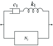
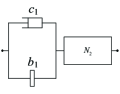
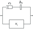
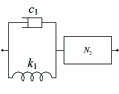
Figure 17: Classes of five-element series-parallel configurations, where $N_{2}$ is a three-element series-parallel subnetwork consisting of one damper and two energy storage elements.

For Fig. 16, $N_{2}$ must consist of one damper and three energy storage elements by Lemmas 3 and 4. By the principle of frequency inversion, assume that $N_{2}$ contains at least two springs. Recalling that $Z(s)$ cannot be realized with fewer than five elements, by Lemma 3, $N_{2}$ cannot be further decomposed as a parallel connection of two subnetworks. Therefore, the network graph of $N_{2}$ can only be one of the graphs in Fig. 19. For the graph in Fig. 19, to avoid $k$-$\mathcal{P}(a,a^{\prime})$ and $b$-$\mathcal{P}(a,a^{\prime})$, Edge 1 and one of Edges 2–4 must correspond to dampers by Lemma 2. Since $N_{2}$ is in parallel with a damper $c_{1}$, by the equivalence in Fig. 18, $Z(s)$ is realizable as a four-element series-parallel network, which contradicts the assumption. For the graph in Fig. 19, recalling that the number of springs is at least two, one of Edges 1 and 2 and one of Edges 3 and 4 must correspond to springs. This means that there exists $k$-$\mathcal{P}(a,a^{\prime})$, which contradicts the assumption by Lemma 2. For the graph in Fig. 19, one of Edges 1 and 2 and one of Edges 3 and 4 must correspond to springs, which based on the equivalence in Fig. 18 implies that the subnetwork $N_{2}$ can always be equivalent to the subnetwork whose network graph is in Fig. 19. Therefore, one only needs to discuss the graph in Fig. 19, which can imply all the possible configurations in Figs. 1, 2, 3, and 4 by Lemma 2 and the approach of enumeration.

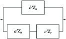
Figure 18: Two networks that are equivalent with each other, where $a^{\prime}=a(a+b)/b$, $b^{\prime}=a+b$, $c^{\prime}=c(a+b)^{2}/b^{2}$, and $Z_{u}$ and $Z_{v}$ are positive-real impedances (see [48]).

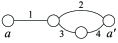
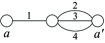
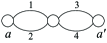
Figure 19: Network graphs of four-element series-parallel subnetworks $N_{2}$ in Fig. 16, where $a$ and $a^{\prime}$ are vertices corresponding to two terminals.

For Fig. 17, $N_{2}$ must consist of one damper and two energy storage elements by Lemmas 3 and 4. By the principle of frequency inversion, assume that $N_{2}$ contains at least one spring. To avoid repeated discussion, the network graph of $N_{2}$ can be one of the graphs in Fig. 20. For the graph in Fig. 20, the network graph of any configuration for Fig. 17 realizing $Z(s)$ must contain $k$-$\mathcal{C}(a,a^{\prime})$, which contradicts the assumption by Lemma 2. For Fig. 20, all the possible configurations are implied in Figs. 5 and 6 by Lemma 2 and the approach of enumeration.

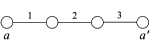
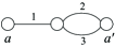
Figure 20: Network graphs of three-element series-parallel subnetworks $N_{2}$ in Fig. 17, where $a$ and $a^{\prime}$ are vertices corresponding to two terminals.

Together with the principles of duality, frequency inversion, and frequency-inverse duality, one can obtain the configurations in Figs. 1–6 covering all the cases, where the configuration in Fig. 1 (resp. Fig. 1) whose one-terminal-pair labeled graph is $\mathcal{N}_{1a}$ (resp. $\text{Dual}(\mathcal{N}_{1a})$) can always be equivalent to the configuration whose one-terminal-pair labeled graph is $\text{GDu}(\mathcal{N}_{1a})$ (resp. $\text{Inv}(\mathcal{N}_{1a})$) by the equivalence in Fig. 18.

Appendix B Proof of Lemma 6

By the principle of duality, one only needs to prove that the impedance $Z(s)$ of this lemma is realizable as in Fig. 1, if and only if $\mathcal{B}_{13}>0$, $\mathcal{B}_{12}=0$, $\mathcal{B}_{23}=0$, and $\Delta_{1}>0$.

Necessity. The impedance of the configuration in Fig. 1 is calculated as $Z(s)=a(s)/d(s)$, where $a(s)=c_{1}^{-1}k_{1}^{-1}k_{2}^{-1}b_{1}s^{3}+c_{1}^{-1}c_{2}^{-1}(k_{1}^{-1}+k_{2}^{-1})b_{1}s^{2}+c_{1}^{-1}k_{1}^{-1}s+c_{1}^{-1}c_{2}^{-1}$ and $d(s)=k_{1}^{-1}k_{2}^{-1}b_{1}s^{3}+(c_{1}^{-1}+c_{2}^{-1})(k_{1}^{-1}+k_{2}^{-1})b_{1}s^{2}+k_{1}^{-1}s+c_{1}^{-1}+c_{2}^{-1}$. Since $Z(s)$ is realizable as the configuration in Fig. 1, it follows that

$$c_{1}^{-1}k_{1}^{-1}k_{2}^{-1}b_{1} =xa_{3},$$ (B.1a)

$$c_{1}^{-1}c_{2}^{-1}(k_{1}^{-1}+k_{2}^{-1})b_{1} =xa_{2},$$ (B.1b)

$$c_{1}^{-1}k_{1}^{-1} =xa_{1},$$ (B.1c)

$$c_{1}^{-1}c_{2}^{-1} =xa_{0},$$ (B.1d)

$$k_{1}^{-1}k_{2}^{-1}b_{1} =xd_{3},$$ (B.1e)

$$(c_{1}^{-1}+c_{2}^{-1})(k_{1}^{-1}+k_{2}^{-1})b_{1} =xd_{2},$$ (B.1f)

$$k_{1}^{-1} =xd_{1},$$ (B.1g)

$$c_{1}^{-1}+c_{2}^{-1} =xd_{0},$$ (B.1h)

where $x>0$. It follows from (B.1a) and (B.1e) that the value of $c_{1}$ can be expressed as in (4). Together with (B.1c) and (B.1g), it is implies that $\mathcal{B}_{23}:=a_{3}d_{1}-a_{1}d_{3}=0$. Then, substituting the expression of $c_{1}$ into (B.1d) and (B.1h) yields

$$x=\frac{a_{3}^{2}}{d_{3}\mathcal{B}_{13}},$$ (B.2)

and the expression of $c_{2}$ as in (4), which by $c_{2}>0$ implies that $\mathcal{B}_{13}:=a_{3}d_{0}-a_{0}d_{3}>0$. From (B.1e) and (B.1g), one derives that

$$k_{2}^{-1}b_{1}=\frac{d_{3}}{d_{1}},$$ (B.3)

From (B.1g) and (B.2), the expression of $k_{1}$ can be derived as in (4). By (B.1b), (B.1d), (B.1f), and (B.1h), one obtains $\mathcal{B}_{12}:=a_{2}d_{0}-a_{0}d_{2}=0$ and $(k_{1}^{-1}+k_{2}^{-1})b_{1}=a_{2}/a_{0}$, which together with (B.3) and the expression of $k_{1}$ implies that

$$k_{2}=\frac{\mathcal{B}_{13}(a_{2}d_{1}-a_{0}d_{3})}{a_{0}a_{3}^{2}d_{1}},~{}~{}b_{1}=\frac{d_{3}\mathcal{B}_{13}(a_{2}d_{1}-a_{0}d_{3})}{a_{0}a_{3}^{2}d_{1}^{2}}.$$ (B.4)

It follows from $\mathcal{B}_{23}=0$ that $a_{3}(a_{2}d_{1}-a_{0}d_{3})=d_{3}\Delta_{1}$, which together with (B.4) implies that the expressions of $k_{2}$ and $b_{1}$ can be further obtained as in (4). Since $\mathcal{B}_{13}>0$ and $k_{2}>0$, it is implied that $\Delta_{1}:=a_{1}a_{2}-a_{0}a_{3}>0$. Therefore, the necessity part is proved.

Sufficiency. Suppose that $\mathcal{B}_{13}>0$, $\mathcal{B}_{12}=0$, $\mathcal{B}_{23}=0$, and $\Delta_{1}>0$. Let the values of the elements satisfy (4) and $x$ satisfy (B.2). Then, $\Delta_{1}>0$ and $\mathcal{B}_{13}>0$ can guarantee that the element values are positive and finite. Since $\mathcal{B}_{12}=0$ and $\mathcal{B}_{23}=0$, it can be verified that conditions (B.1a)–(B.1h) hold. Therefore, $Z(s)$ is realizable as the configuration in Fig. 1.

Appendix C Proof of Lemma 11

By the principles of duality, frequency inversion, and frequency-inverse duality, one only needs to prove that the impedance $Z(s)$ of this lemma is realizable as the configuration in Fig. 6, if and only if Condition 1 of this lemma holds, where $\zeta_{1}$ is defined in (9).

Necessity. The impedance of the configuration in Fig. 6 is calculated as $Z(s)=a(s)/d(s)$, where $a(s)=c_{2}^{-1}k_{1}^{-1}k_{2}^{-1}b_{1}s^{3}+(c_{1}^{-1}c_{2}^{-1}b_{1}+k_{1}^{-1})k_{2}^{-1}s^{2}+(c_{1}^{-1}k_{2}^{-1}+c_{2}^{-1}k_{1}^{-1})s+c_{1}^{-1}c_{2}^{-1}$ and $d(s)=k_{1}^{-1}k_{2}^{-1}b_{1}s^{3}+(c_{1}^{-1}k_{2}^{-1}+c_{2}^{-1}k_{1}^{-1}+c_{2}^{-1}k_{2}^{-1})s^{2}+(c_{1}^{-1}c_{2}^{-1}b_{1}+k_{2}^{-1})s+c_{2}^{-1}$. Since $Z(s)$ is realizable as the configuration in Fig. 6, it follows that

$$c_{2}^{-1}k_{1}^{-1}k_{2}^{-1}b_{1} =xa_{3},$$ (C.1a)

$$(c_{1}^{-1}c_{2}^{-1}b_{1}+k_{1}^{-1})k_{2}^{-1} =xa_{2},$$ (C.1b)

$$c_{1}^{-1}k_{2}^{-1}+c_{2}^{-1}k_{1}^{-1} =xa_{1},$$ (C.1c)

$$c_{1}^{-1}c_{2}^{-1} =xa_{0},$$ (C.1d)

$$k_{1}^{-1}k_{2}^{-1}b_{1} =xd_{3},$$ (C.1e)

$$c_{1}^{-1}k_{2}^{-1}+c_{2}^{-1}k_{1}^{-1}+c_{2}^{-1}k_{2}^{-1} =xd_{2},$$ (C.1f)

$$c_{1}^{-1}c_{2}^{-1}b_{1}+k_{2}^{-1} =xd_{1},$$ (C.1g)

$$c_{2}^{-1} =xd_{0},$$ (C.1h)

where $x>0$. Then, it follows from (C.1a) and (C.1e) that the expression of $c_{2}$ can be obtained as in (10), which together with (C.1d) and (C.1h) implies

$$x=\frac{a_{3}}{d_{0}d_{3}},$$ (C.2)

and the expression of $c_{1}$ as in (10). It is implied from (C.1c) and (C.1g) that

$$k_{1}=\frac{a_{3}d_{0}}{a_{1}a_{3}-a_{0}d_{3}k_{2}^{-1}},~{}~{}~{}b_{1}=\frac{a_{3}d_{1}-d_{0}d_{3}k_{2}^{-1}}{a_{0}a_{3}}.$$ (C.3)

Substituting (C.2), (C.3), and the expressions of $c_{1}$ and $c_{2}$ into (C.1f) yields $d_{0}^{2}d_{3}k_{2}^{-2}-d_{0}\mathcal{B}_{23}k_{2}^{-1}-a_{3}(a_{1}d_{1}-a_{0}d_{2})=0$, which implies that $\mathcal{M}_{23}^{2}-4a_{0}a_{3}d_{2}d_{3}\geq 0$ and $k_{2}=a_{0}d_{0}d_{3}/(a_{3}\zeta_{1})$ as in (10), where $\zeta_{1}$ is defined in (9). Furthermore, substituting $k_{2}=a_{0}d_{0}d_{3}/(a_{3}\zeta_{1})$ into (C.3) implies that the element values of $k_{1}$ and $b_{1}$ can be expressed as in (10). By the assumption that $k_{1}>0$, $k_{2}>0$, and $b_{1}>0$, it is implied that $0<\zeta_{1}<\min\{a_{1}d_{0},a_{0}d_{1}\}$. Substituting the element values in (10) and $x$ in (C.2) into (C.1b) and (C.1e) can imply $a_{3}\zeta_{1}^{2}-a_{0}\mathcal{B}_{23}\zeta_{1}-a_{0}^{2}d_{3}(a_{1}d_{1}-a_{0}d_{2})=0$ and $\zeta_{1}^{3}-\mathcal{M}_{11}\zeta_{1}^{2}+a_{0}a_{1}d_{0}d_{1}\zeta_{1}-a_{0}^{3}d_{0}^{2}d_{3}=0$. Therefore, the necessity part is proved.

Sufficiency. Suppose that Condition 1 of this lemma holds. Let the values of the elements satisfy (10) and $x$ satisfy (C.2). Then, $0<\zeta_{1}<\min\{a_{1}d_{0},a_{0}d_{1}\}$ and $\mathcal{M}_{23}^{2}-4a_{0}a_{3}d_{2}d_{3}\geq 0$ can guarantee that the element values are positive and finite. Since $a_{3}\zeta_{1}^{2}-a_{0}\mathcal{B}_{23}\zeta_{1}-a_{0}^{2}d_{3}(a_{1}d_{1}-a_{0}d_{2})=0$ and $\zeta_{1}^{3}-\mathcal{M}_{11}\zeta_{1}^{2}+a_{0}a_{1}d_{0}d_{1}\zeta_{1}-a_{0}^{3}d_{0}^{2}d_{3}=0$, it can be verified that conditions (C.1a)–(C.1h) hold. Therefore, $Z(s)$ is realizable as the configuration in Fig. 6.

Appendix D Proof of Lemma 12

Sufficiency. The sufficiency part is clearly satisfied.

Necessity. Since there is no pole or zero on $j\mathbb{R}\cup\infty$, there are at most four energy storage elements. Together with Lemma 4, the number of energy storage elements is either three or four. By Lemma 2 and the approach of enumeration, all the possible configurations are as in Figs. 7–11 and 21. It remains to discussing the realizability of $Z(s)$ in this lemma as the five-element configurations containing four energy storage elements in Figs. 11 and 21.

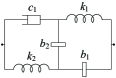
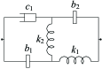
Figure 21: Five-element non-series-parallel configurations that cannot realize the bicubic impedance $Z(s)$ in (1), whose one-terminal-pair labeled graphs are (a) $\mathcal{N}_{12a}$ and (b) $\mathcal{N}_{12b}$, respectively, satisfying $\mathcal{N}_{12b}=\text{Dual}(\mathcal{N}_{12a})$, where $\text{Inv}(\mathcal{N}_{12a})=\text{Dual}(\mathcal{N}_{12a})$ and $\text{GDu}(\mathcal{N}_{12a})=\mathcal{N}_{12a}$.

The impedance of the five-element configuration containing four energy storage elements in Fig. 11 is calculated as $Z(s)=a(s)/d(s)$, where $a(s)=c_{1}^{-1}k_{1}^{-1}k_{2}^{-1}b_{1}b_{2}s^{4}+k_{1}^{-1}k_{2}^{-1}(b_{1}+b_{2})s^{3}+c_{1}^{-1}(k_{1}^{-1}b_{1}+k_{2}^{-1}b_{2})s^{2}+(k_{1}^{-1}+k_{2}^{-1})s+c_{1}^{-1}$ and $d(s)=k_{1}^{-1}k_{2}^{-1}b_{1}b_{2}s^{4}+c_{1}^{-1}(k_{1}^{-1}+k_{2}^{-1})b_{1}b_{2}s^{3}+(k_{1}^{-1}b_{2}+k_{2}^{-1}b_{1})s^{2}+c_{1}^{-1}(b_{1}+b_{2})s+1$. Choosing $k_{1}=1/16$ $\text{N}/\text{m}$, $k_{2}=1$ $\text{N}/\text{m}$, $b_{1}=1$ kg, $b_{2}=1$ kg, and $c_{1}=1/2$ $\text{Ns}/\text{m}$, the impedance of Fig. 11 is $Z(s)=(16s^{3}+8s^{2}+13s+2)/(8s^{3}+13s^{2}+2s+1)$, which satisfies the assumption. Therefore, the configuration in Fig. 11 can realize the bicubic impedance in (1) for some element values.

The impedance of the five-element configuration containing four energy storage elements in Fig. 21 is calculated as $Z(s)=a(s)/d(s)$, where $a(s)=c_{1}^{-1}k_{1}^{-1}k_{2}^{-1}b_{1}b_{2}s^{4}+k_{1}^{-1}k_{2}^{-1}(b_{1}+b_{2})s^{3}+c_{1}^{-1}(k_{1}^{-1}b_{2}+k_{2}^{-1}b_{1}+k_{2}^{-1}b_{2})s^{2}+k_{1}^{-1}s+c_{1}^{-1}$ and $d(s)=k_{1}^{-1}k_{2}^{-1}b_{1}b_{2}s^{4}+c_{1}^{-1}k_{1}^{-1}b_{1}b_{2}s^{3}+(k_{1}^{-1}b_{1}+k_{2}^{-1}b_{1}+k_{2}^{-1}b_{2})s^{2}+c_{1}^{-1}(b_{1}+b_{2})s+1$. Assume that a bicubic impedance of this lemma is realizable as the configuration in Fig. 21. Then, the resultant [49, Chapter XV] of $a(s)$ and $d(s)$ in $s$ calculated as $R_{0}(a,b,s)=k_{1}^{-3}k_{2}^{-1}b_{1}b_{2}h_{2}^{2}$ must be zero, where $h_{2}:=k_{1}^{-1}b_{1}b_{2}^{3}c_{1}^{-4}+k_{2}^{-1}(b_{1}+b_{2})(k_{2}^{-1}(b_{1}+b_{2})^{2}-3k_{1}^{-1}b_{1}b_{2})c_{1}^{-2}+k_{1}^{-2}k_{2}^{-1}b_{1}^{2}$. If $k_{2}^{-1}(b_{1}+b_{2})^{2}-3k_{1}^{-1}b_{1}b_{2}\geq 0$, then $h_{2}>0$, which implies that $R_{0}(a,b,s)>0$. This contradicts the assumption. If $k_{2}^{-1}(b_{1}+b_{2})^{2}-3k_{1}^{-1}b_{1}b_{2}<0$, then the discriminant of the equation $h_{2}=0$ in $c_{1}^{-2}$ is calculated as $(k_{2}^{-1}(b_{1}+b_{2})(k_{2}^{-1}(b_{1}+b_{2})^{2}-3k_{1}^{-1}b_{1}b_{2}))^{2}-4k_{1}^{-1}b_{1}b_{2}^{3}k_{1}^{-2}k_{2}^{-1}b_{1}^{2}=k_{2}^{-1}(k_{2}^{-1}(b_{1}+b_{2})^{2}-4k_{1}^{-1}b_{1}b_{2})(k_{2}^{-1}(b_{1}+b_{2})^{2}-k_{1}^{-1}b_{1}b_{2})^{2}\leq 0$. Since $h_{2}=0$ must have a positive root in $c_{2}^{-2}$, it is implied that $k_{2}^{-1}(b_{1}+b_{2})^{2}-k_{1}^{-1}b_{1}b_{2}=0$, which together with $h_{2}=0$ implies $c_{1}^{2}=b_{2}^{-2}/(k_{2}^{-1}(b_{1}+b_{2}))$. Therefore, the impedance becomes $Z(s)=c_{1}^{-1}(c_{1}^{-2}b_{1}b_{2}^{2}s^{2}+c_{1}^{-1}b_{2}^{2}s+b_{1})/(b_{1}(c_{1}^{-2}b_{2}^{2}s^{2}+c_{1}^{-1}b_{1}s+1))$, whose McMillan degree is at most two. By contradiction, any bicubic impedance of this lemma cannot be realized as the configuration in Fig. 21, which cannot be realized as the configuration in Fig. 21 by the principle of duality.

Appendix E Proof of Lemma 14

By the principle of duality, one only needs to prove that the impedance $Z(s)$ of this lemma is realizable as the configuration in Fig. 8, if and only if Condition 1 or Condition 2 of this lemma holds, where $\Lambda_{1a}$ and $\Lambda_{1b}$ are defined in (12) and (13), respectively.

Necessity. The impedance of the configuration in Fig. 8 is calculated as $Z(s)=a(s)/d(s)$, where $a(s)=c_{2}^{-1}k_{1}^{-1}k_{2}^{-1}b_{1}s^{3}+(c_{1}^{-1}c_{2}^{-1}(k_{1}^{-1}+k_{2}^{-1})b_{1}+k_{1}^{-1}k_{2}^{-1})s^{2}+(c_{1}^{-1}(k_{1}^{-1}+k_{2}^{-1})+c_{2}^{-1}k_{1}^{-1})s+c_{1}^{-1}c_{2}^{-1}$ and $d(s)=k_{1}^{-1}k_{2}^{-1}b_{1}s^{3}+(c_{1}^{-1}(k_{1}^{-1}+k_{2}^{-1})+c_{2}^{-1}k_{2}^{-1})b_{1}s^{2}+(c_{1}^{-1}c_{2}^{-1}b_{1}+k_{1}^{-1}+k_{2}^{-1})s+c_{2}^{-1}$. Then,

$$c_{2}^{-1}k_{1}^{-1}k_{2}^{-1}b_{1} =xa_{3},$$ (E.1a)

$$c_{1}^{-1}c_{2}^{-1}(k_{1}^{-1}+k_{2}^{-1})b_{1}+k_{1}^{-1}k_{2}^{-1} =xa_{2},$$ (E.1b)

$$c_{1}^{-1}(k_{1}^{-1}+k_{2}^{-1})+c_{2}^{-1}k_{1}^{-1} =xa_{1},$$ (E.1c)

$$c_{1}^{-1}c_{2}^{-1} =xa_{0},$$ (E.1d)

$$k_{1}^{-1}k_{2}^{-1}b_{1} =xd_{3},$$ (E.1e)

$$(c_{1}^{-1}(k_{1}^{-1}+k_{2}^{-1})+c_{2}^{-1}k_{2}^{-1})b_{1} =xd_{2},$$ (E.1f)

$$c_{1}^{-1}c_{2}^{-1}b_{1}+k_{1}^{-1}+k_{2}^{-1} =xd_{1},$$ (E.1g)

$$c_{2}^{-1} =xd_{0},$$ (E.1h)

where $x>0$. It follows from (E.1a) and (E.1e) that the expression of $c_{2}$ can be obtained as in (14), together with (E.1d) and (E.1h) yields the expression of $c_{1}$ as in (14) and

$$x=\frac{a_{3}}{d_{0}d_{3}}.$$ (E.2)

Substituting (E.2) and the expressions of $c_{1}$ and $c_{2}$ into (E.1g) yields

$$k_{1}^{-1}+k_{2}^{-1}=\frac{a_{3}(d_{1}-a_{0}b_{1})}{d_{0}d_{3}},$$ (E.3)

which together with (E.1c) and (E.1e) implies the expressions of $k_{1}$ and $k_{2}$ as in (14). Substituting (E.2), and the expressions of $c_{2}$, $k_{1}$ and $k_{2}$ into (E.1b) implies

$$c_{1}^{-1}(k_{1}^{-1}+k_{2}^{-1})b_{1}=\frac{a_{2}b_{1}-d_{3}}{d_{0}b_{1}}.$$ (E.4)

Substituting (E.2), (E.4), and the expressions of $c_{2}$ and $k_{2}$ into (E.1f) implies $a_{0}^{2}\mathcal{B}_{33}b_{1}^{2}-(\mathcal{B}_{13}\mathcal{M}_{13}-\mathcal{B}_{11}\mathcal{B}_{33})b_{1}+d_{3}^{2}\mathcal{B}_{11}=0$. If $\mathcal{B}_{33}=0$, then $b_{1}$ must satisfy $b_{1}=\Lambda_{1a}$, where $\Lambda_{1a}$ is defined in (12). Then, $b_{1}>0$ implies that $\mathcal{B}_{11}\mathcal{B}_{13}>0$. Together with the element values in (14) and $x$ in (E.2), it follows from (E.1b) and (E.3) that $a_{0}^{2}a_{3}\Lambda_{1a}^{3}-a_{0}a_{3}d_{1}\Lambda_{1a}^{2}+a_{2}d_{0}d_{3}\Lambda_{1a}-d_{0}d_{3}^{2}=0$ and $a_{0}^{3}\mathcal{M}_{13}\Lambda_{1a}^{3}+a_{0}(2\mathcal{B}_{11}\mathcal{M}_{13}+a_{1}a_{3}d_{0}^{2})\Lambda_{1a}^{2}+\mathcal{B}_{11}(d_{3}\mathcal{B}_{11}-a_{3}d_{0}d_{1})\Lambda_{1a}+a_{3}d_{0}^{3}d_{3}=0$. If $\mathcal{B}_{33}\neq 0$, then $(\mathcal{B}_{13}^{2}-\mathcal{B}_{11}\mathcal{B}_{33})(\mathcal{M}_{13}^{2}-\mathcal{B}_{11}\mathcal{B}_{33})\geq 0$, and $b_{1}$ can be solved as $b_{1}=\Lambda_{1b}$, where $\Lambda_{1b}$ is defined in (13), which by $k_{1}>0$ and $k_{2}>0$ implies that $a_{0}^{2}\Lambda_{1b}>\max\{0,-\mathcal{B}_{11}\}$. Similarly, together with the element values in (14) and $x$ in (E.2), it follows from (E.1b) and (E.3) that $a_{0}^{2}a_{3}\Lambda_{1b}^{3}-a_{0}a_{3}d_{1}\Lambda_{1b}^{2}+a_{2}d_{0}d_{3}\Lambda_{1b}-d_{0}d_{3}^{2}=0$ and $a_{0}^{3}\mathcal{M}_{13}\Lambda_{1b}^{3}+a_{0}(2\mathcal{B}_{11}\mathcal{M}_{13}+a_{1}a_{3}d_{0}^{2})\Lambda_{1b}^{2}+\mathcal{B}_{11}(d_{3}\mathcal{B}_{11}-a_{3}d_{0}d_{1})\Lambda_{1b}+a_{3}d_{0}^{3}d_{3}=0$.

Sufficiency. Suppose that Condition 1 of this lemma holds. Let $c_{1}$, $c_{2}$, $k_{1}$, and $k_{2}$ satisfy (14), $b_{1}=\Lambda_{1a}$, and $x$ satisfy (E.2). Then, $\mathcal{B}_{11}\mathcal{B}_{13}>0$ implies that $\Lambda_{1a}=d_{3}^{3}\mathcal{B}_{11}/(\mathcal{B}_{13}\mathcal{M}_{13})>0$ and $a_{0}^{2}\Lambda_{1a}+\mathcal{B}_{11}=a_{3}^{2}d_{0}^{2}\mathcal{B}_{11}/(\mathcal{B}_{13}\mathcal{M}_{13})>0$, which can guarantee that the element values are positive and finite. Since $\mathcal{B}_{33}=0$, $a_{0}^{2}a_{3}\Lambda_{1a}^{3}-a_{0}a_{3}d_{1}\Lambda_{1a}^{2}+a_{2}d_{0}d_{3}\Lambda_{1a}-d_{0}d_{3}^{2}=0$, and $a_{0}^{3}\mathcal{M}_{13}\Lambda_{1a}^{3}+a_{0}(2\mathcal{B}_{11}\mathcal{M}_{13}+a_{1}a_{3}d_{0}^{2})\Lambda_{1a}^{2}+\mathcal{B}_{11}(d_{3}\mathcal{B}_{11}-a_{3}d_{0}d_{1})\Lambda_{1a}+a_{3}d_{0}^{3}d_{3}=0$, it can be verified that conditions (E.1a)–(E.1h) hold. Therefore, $Z(s)$ is realizable as the configuration in Fig. 8. Similar discussions can be made when Condition 2 of this lemma holds.

Appendix F Proof of Lemma 15

By the principle of duality, one only needs to prove that the impedance $Z(s)$ of this lemma is realizable as the configuration in Fig. 9, if and only if Condition 1 of this lemma holds, where $\Gamma_{1}$ and $\Phi_{1}$ are defined in (15) and (16), respectively.

Necessity. The impedance of the configuration in Fig. 9 is calculated as $Z(s)=a(s)/d(s)$, where $a(s)=(c_{1}^{-1}+c_{2}^{-1})k_{1}^{-1}k_{2}^{-1}b_{1}s^{3}+(c_{1}^{-1}c_{2}^{-1}(k_{1}^{-1}+k_{2}^{-1})b_{1}+k_{1}^{-1}k_{2}^{-1})s^{2}+(c_{1}^{-1}k_{2}^{-1}+c_{2}^{-1}k_{1}^{-1})s+c_{1}^{-1}c_{2}^{-1}$ and $d(s)=k_{1}^{-1}k_{2}^{-1}b_{1}s^{3}+(c_{1}^{-1}k_{1}^{-1}+c_{2}^{-1}k_{2}^{-1})b_{1}s^{2}+(c_{1}^{-1}c_{2}^{-1}b_{1}+k_{1}^{-1}+k_{2}^{-1})s+c_{1}^{-1}+c_{2}^{-1}$. Then,

$$(c_{1}^{-1}+c_{2}^{-1})k_{1}^{-1}k_{2}^{-1}b_{1} =xa_{3},$$ (F.1a)

$$c_{1}^{-1}c_{2}^{-1}(k_{1}^{-1}+k_{2}^{-1})b_{1}+k_{1}^{-1}k_{2}^{-1} =xa_{2},$$ (F.1b)

$$c_{1}^{-1}k_{2}^{-1}+c_{2}^{-1}k_{1}^{-1} =xa_{1},$$ (F.1c)

$$c_{1}^{-1}c_{2}^{-1} =xa_{0},$$ (F.1d)

$$k_{1}^{-1}k_{2}^{-1}b_{1} =xd_{3},$$ (F.1e)

$$(c_{1}^{-1}k_{1}^{-1}+c_{2}^{-1}k_{2}^{-1})b_{1} =xd_{2},$$ (F.1f)

$$c_{1}^{-1}c_{2}^{-1}b_{1}+k_{1}^{-1}+k_{2}^{-1} =xd_{1},$$ (F.1g)

$$c_{1}^{-1}+c_{2}^{-1} =xd_{0},$$ (F.1h)

where $x>0$. It follows from (F.1a) and (F.1e) that

$$c_{1}^{-1}+c_{2}^{-1}=\frac{a_{3}}{d_{3}},$$ (F.2)

which together with (F.1h) implies that

$$x=\frac{a_{3}}{d_{0}d_{3}}.$$ (F.3)

By (F.1d), (F.2), and (F.3), one implies that $d_{0}d_{3}c_{1}^{-2}-a_{3}d_{0}c_{1}^{-1}+a_{0}a_{3}=0$, $c_{2}^{-1}=a_{0}a_{3}/(d_{0}d_{3}c_{1}^{-1})$, and $c_{2}^{-1}=a_{3}/d_{3}-c_{1}^{-1}$. Furthermore, $a_{3}d_{0}-4a_{0}d_{3}\geq 0$, and one obtains $c_{1}=1/\Gamma_{1}$ and $c_{2}=d_{0}d_{3}\Gamma_{1}/(a_{0}a_{3})$ as in (18), where $\Gamma_{1}$ is defined in (15). Substituting (F.1d) and (F.3) into (F.1c) and (F.1e) yields

$$k_{2}=\frac{d_{0}d_{3}c_{1}^{-2}}{a_{3}(a_{1}c_{1}^{-1}-a_{0}k_{1}^{-1})},~{}~{}b_{1}=\frac{d_{3}c_{1}^{-2}}{(a_{1}c_{1}^{-1}-a_{0}k_{1}^{-1})k_{1}^{-1}}.$$ (F.4)

Substituting (F.3), (F.4), $c_{1}=1/\Gamma_{1}$, and $c_{2}=d_{0}d_{3}\Gamma_{1}/(a_{0}a_{3})$ into (F.1f) yields $a_{0}a_{3}d_{0}d_{2}\Gamma_{1}k_{1}^{-2}+(d_{0}^{2}d_{3}^{2}\Gamma_{1}^{4}-a_{1}a_{3}d_{0}d_{2}\Gamma_{1}^{2}-a_{0}^{2}a_{3}^{2})k_{1}^{-1}+a_{0}a_{1}a_{3}^{2}\Gamma_{1}=0$, which implies that $(a_{1}a_{3}d_{0}d_{2}\Gamma_{1}^{2}-(d_{0}d_{3}\Gamma_{1}^{2}-a_{0}a_{3})^{2})(a_{1}a_{3}d_{0}d_{2}\Gamma_{1}^{2}-(d_{0}d_{3}\Gamma_{1}^{2}+a_{0}a_{3})^{2})\geq 0$ and $k_{1}=1/\Phi_{1}$ as in (18), where $\Phi_{1}$ is defined in (16). Furthermore, substituting $c_{1}=1/\Gamma_{1}$, $c_{2}=d_{0}d_{3}\Gamma_{1}/(a_{0}a_{3})$, and $k_{1}=1/\Phi_{1}$ into (F.4) implies the expressions of $k_{2}$ and $b_{1}$ as in (18). The assumption that the element values are positive and finite implies that $0<\Phi_{1}/\Gamma_{1}<a_{1}/a_{0}$. By the element values in (18) and $x$ in (F.3), it follows from (F.1b) and (F.1g) that $a_{0}^{2}d_{0}\Phi_{1}^{4}-2a_{0}a_{1}d_{0}\Gamma_{1}\Phi_{1}^{3}+d_{0}(a_{1}^{2}+a_{0}a_{2})\Gamma_{1}^{2}\Phi_{1}^{2}+(a_{0}d_{0}d_{3}\Gamma_{1}^{2}-a_{1}a_{2}d_{0}\Gamma_{1}-a_{0}^{2}a_{3})\Gamma_{1}^{2}\Phi_{1}+a_{0}a_{1}a_{3}\Gamma_{1}^{3}=0$ and $a_{0}(d_{0}d_{3}\Gamma_{1}^{2}-a_{0}a_{3})\Phi_{1}^{3}-(a_{1}d_{0}d_{3}\Gamma_{1}^{2}+a_{0}a_{3}d_{1}\Gamma_{1}-2a_{0}a_{1}a_{3})\Gamma_{1}\Phi_{1}^{2}+a_{1}a_{3}(d_{1}\Gamma_{1}-a_{1})\Gamma_{1}^{2}\Phi_{1}-a_{0}a_{3}d_{3}\Gamma_{1}^{4}=0$ hold.

Sufficiency. Suppose that Condition 1 of this lemma holds. Let the values of the elements satisfy (18) and $x$ satisfy (F.3). Since $0<\Phi_{1}/\Gamma_{1}<a_{1}/a_{0}$, $a_{3}d_{0}-4a_{0}d_{3}\geq 0$, $(a_{1}a_{3}d_{0}d_{2}\Gamma_{1}^{2}-(d_{0}d_{3}\Gamma_{1}^{2}-a_{0}a_{3})^{2})(a_{1}a_{3}d_{0}d_{2}\Gamma_{1}^{2}-(d_{0}d_{3}\Gamma_{1}^{2}+a_{0}a_{3})^{2})\geq 0$, it is clear that the element values as in (18) can be positive and finite. Since $a_{0}(d_{0}d_{3}\Gamma_{1}^{2}-a_{0}a_{3})\Phi_{1}^{3}-(a_{1}d_{0}d_{3}\Gamma_{1}^{2}+a_{0}a_{3}d_{1}\Gamma_{1}-2a_{0}a_{1}a_{3})\Gamma_{1}\Phi_{1}^{2}+a_{1}a_{3}(d_{1}\Gamma_{1}-a_{1})\Gamma_{1}^{2}\Phi_{1}-a_{0}a_{3}d_{3}\Gamma_{1}^{4}=0$, and $a_{0}^{2}d_{0}\Phi_{1}^{4}-2a_{0}a_{1}d_{0}\Gamma_{1}\Phi_{1}^{3}+d_{0}(a_{1}^{2}+a_{0}a_{2})\Gamma_{1}^{2}\Phi_{1}^{2}+(a_{0}d_{0}d_{3}\Gamma_{1}^{2}-a_{1}a_{2}d_{0}\Gamma_{1}-a_{0}^{2}a_{3})\Gamma_{1}^{2}\Phi_{1}+a_{0}a_{1}a_{3}\Gamma_{1}^{3}=0$, it can be verified that conditions (F.1a)–(F.1h) hold. Therefore, $Z(s)$ is realizable as the configuration in Fig. 9.

Appendix G Proof of Lemma 17

Necessity. The impedance of the configuration in Fig. 11 is calculated as $Z(s)=a(s)/d(s)$, where $a(s)=k_{1}^{-1}k_{2}^{-1}b_{1}b_{2}s^{4}+c_{1}^{-1}(k_{1}^{-1}+k_{2}^{-1})b_{1}b_{2}s^{3}+(k_{1}^{-1}b_{2}+k_{2}^{-1}b_{1})s^{2}+c_{1}^{-1}(b_{1}+b_{2})s+1$ and $d(s)=c_{1}^{-1}k_{1}^{-1}k_{2}^{-1}b_{1}b_{2}s^{4}+k_{1}^{-1}k_{2}^{-1}(b_{1}+b_{2})s^{3}+c_{1}^{-1}(k_{1}^{-1}b_{1}+k_{2}^{-1}b_{2})s^{2}+(k_{1}^{-1}+k_{2}^{-1})s+c_{1}^{-1}$. Then, multiplying the numerator and denominator of the bicubic impedance $Z(s)$ in (1) with a common factor $(Ts+1)$ where $T>0$, it follows that

$$c_{1}^{-1}k_{1}^{-1}k_{2}^{-1}b_{1}b_{2} =xa_{3}T,$$ (G.1a)

$$k_{1}^{-1}k_{2}^{-1}(b_{1}+b_{2}) =x(a_{2}T+a_{3}),$$ (G.1b)

$$c_{1}^{-1}(k_{1}^{-1}b_{1}+k_{2}^{-1}b_{2}) =x(a_{1}T+a_{2}),$$ (G.1c)

$$k_{1}^{-1}+k_{2}^{-1} =x(a_{0}T+a_{1}),$$ (G.1d)

$$c_{1}^{-1} =xa_{0},$$ (G.1e)

$$k_{1}^{-1}k_{2}^{-1}b_{1}b_{2} =xd_{3}T,$$ (G.1f)

$$c_{1}^{-1}(k_{1}^{-1}+k_{2}^{-1})b_{1}b_{2} =x(d_{2}T+d_{3}),$$ (G.1g)

$$k_{1}^{-1}b_{2}+k_{2}^{-1}b_{1} =x(d_{1}T+d_{2}),$$ (G.1h)

$$c_{1}^{-1}(b_{1}+b_{2}) =x(d_{0}T+d_{1}),$$ (G.1i)

$$1 =xd_{0},$$ (G.1j)

where $x>0$. It follows from (G.1a) and (G.1f) that the expression of $c_{1}$ can be expressed as in (22). The expression of $x$ can be directly obtained from (G.1j) as

$$x=\frac{1}{d_{0}}.$$ (G.2)

Then, substituting (G.2) and the expression of $c_{1}$ into (G.1e) implies that $\mathcal{B}_{13}=0$. Furthermore, it follows from (G.1d) that

$$k_{1}^{-1}+k_{2}^{-1}=\frac{a_{0}T+a_{1}}{d_{0}},$$ (G.3)

which together with (G.1g), (G.2), and the expression of $c_{1}$ implies that

$$b_{1}b_{2}=\frac{d_{3}(d_{2}T+d_{3})}{a_{3}(a_{0}T+a_{1})}.$$ (G.4)

Then, substituting (G.2) and (G.4) into (G.1f) yields

$$k_{1}^{-1}k_{2}^{-1}=\frac{a_{3}T(a_{0}T+a_{1})}{d_{0}(d_{2}T+d_{3})},$$ (G.5)

which together with (G.1b) and (G.2) implies that

$$b_{1}+b_{2}=\frac{(a_{2}T+a_{3})(d_{2}T+d_{3})}{a_{3}T(a_{0}T+a_{1})}.$$ (G.6)

By (G.3) and (G.5), it is implied that $k_{1}=1/y_{1}$ and $k_{2}=1/y_{2}$ are two positive roots of equation (20) in $y$, whose discriminant must be nonnegative. Therefore, it follows that $a_{0}d_{2}T^{2}+(a_{1}d_{2}-3a_{0}d_{3})T+a_{1}d_{3}\geq 0$. Similarly, by (G.4) and (G.6), it is implied that $b_{1}=z_{1}$ and $b_{2}=z_{2}$ are two positive roots of equation (21) in $z$, whose discriminant must be nonnegative. Therefore, it follows that $(a_{2}^{2}d_{2}-4a_{0}a_{3}d_{3})T^{3}+(a_{2}^{2}d_{3}+2a_{2}a_{3}d_{2}-4a_{1}a_{3}d_{3})T^{2}+a_{3}(a_{3}d_{2}+2a_{2}d_{3})T+a_{3}^{2}d_{3}\geq 0$. Substituting (G.2), (G.6), and the expression of $c_{1}$ into (G.1i) implies $a_{0}d_{0}d_{3}T^{3}+(a_{1}d_{0}d_{3}+a_{0}d_{1}d_{3}-a_{2}d_{0}d_{2})T^{2}+(a_{1}d_{1}d_{3}-a_{2}d_{0}d_{3}-a_{3}d_{0}d_{2})T-a_{3}d_{0}d_{3}=0$. Substituting (G.1e), (G.2), $k_{1}=1/y_{1}$, $k_{2}=1/y_{2}$, $b_{1}=z_{1}$, and $b_{2}=z_{2}$ into (G.1c) and (G.1h) implies $a_{1}T+a_{2}-a_{0}(y_{1}z_{1}+y_{2}z_{2})=0$ and $d_{1}T+d_{2}-d_{0}(y_{1}z_{2}+y_{2}z_{1})=0$.

Sufficiency. Suppose that the condition of this lemma holds. Then, $a_{0}d_{2}T^{2}+(a_{1}d_{2}-3a_{0}d_{3})T+a_{1}d_{3}\geq 0$ can imply that equation (20) in $y$ has two positive roots denoted as $y_{1}$ and $y_{2}$, and $(a_{2}^{2}d_{2}-4a_{0}a_{3}d_{3})T^{3}+(a_{2}^{2}d_{3}+2a_{2}a_{3}d_{2}-4a_{1}a_{3}d_{3})T^{2}+a_{3}(a_{3}d_{2}+2a_{2}d_{3})T+a_{3}^{2}d_{3}\geq 0$ can imply that equation (21) in $z$ has two positive roots denoted as $z_{1}$ and $z_{2}$. Let the element values satisfy (22), and $x$ satisfy (G.2), which implies that the element values can be positive and finite. Since $\mathcal{B}_{13}=0$, $a_{0}d_{0}d_{3}T^{3}+(a_{1}d_{0}d_{3}+a_{0}d_{1}d_{3}-a_{2}d_{0}d_{2})T^{2}+(a_{1}d_{1}d_{3}-a_{2}d_{0}d_{3}-a_{3}d_{0}d_{2})T-a_{3}d_{0}d_{3}=0$, $a_{1}T+a_{2}-a_{0}(y_{1}z_{1}+y_{2}z_{2})=0$, and $d_{1}T+d_{2}-d_{0}(y_{1}z_{2}+y_{2}z_{1})=0$ imply that (G.3)–(G.6) hold, it can be verified that conditions (G.1a)–(G.1j) hold. Therefore, $Z(s)$ is realizable as the configuration in Fig. 11.

Supplementary Material to: Passive Mechanical Realizations of Bicubic Impedances with No More Than Five Elements for Inerter-Based Control Design

Kai Wang   and  Michael Z. Q. Chen

1 Introduction

This report presents the proofs of some results in the paper entitled “Passive network realizations of bicubic impedances with no more than five elements for inerter-based control design” [1], which are omitted from the paper for brevity. It is assumed that the numbering of lemmas, theorems, equations and figures in this report agrees with that in the original paper.

2 Proof of Lemma 7

By the principles of duality, frequency inversion, and frequency-inverse duality, one only needs to prove that the impedance $Z(s)$ of this lemma is realizable as the configuration in Fig. 2(a), if and only if $\mathcal{B}_{13}=0$, $\Delta_{1}>0$, and $a_{0}\mathcal{B}_{33}=a_{1}\mathcal{B}_{23}>0$.

Necessity. Suppose that $Z(s)$ is realizable as the configuration in Fig. 2(a). The impedance of the configuration in Fig. 2(a) is calculated as $Z(s)=a(s)/d(s)$, where $a(s)=c_{1}^{-1}k_{1}^{-1}k_{2}^{-1}b_{1}s^{3}+c_{1}^{-1}c_{2}^{-1}k_{1}^{-1}b_{1}s^{2}+c_{1}^{-1}(k_{1}^{-1}+k_{2}^{-1})s+c_{1}^{-1}c_{2}^{-1}$ and $d(s)=k_{1}^{-1}k_{2}^{-1}b_{1}s^{3}+(c_{1}^{-1}k_{1}^{-1}+c_{1}^{-1}k_{2}^{-1}+c_{2}^{-1}k_{1}^{-1})b_{1}s^{2}+(c_{1}^{-1}c_{2}^{-1}b_{1}+k_{1}^{-1}+k_{2}^{-1})s+c_{2}^{-1}$. Then, it follows that

$$c_{1}^{-1}k_{1}^{-1}k_{2}^{-1}b_{1} =xa_{3},$$ (2.1a)

$$c_{1}^{-1}c_{2}^{-1}k_{1}^{-1}b_{1} =xa_{2},$$ (2.1b)

$$c_{1}^{-1}(k_{1}^{-1}+k_{2}^{-1}) =xa_{1},$$ (2.1c)

$$c_{1}^{-1}c_{2}^{-1} =xa_{0},$$ (2.1d)

$$k_{1}^{-1}k_{2}^{-1}b_{1} =xd_{3},$$ (2.1e)

$$(c_{1}^{-1}k_{1}^{-1}+c_{1}^{-1}k_{2}^{-1}+c_{2}^{-1}k_{1}^{-1})b_{1} =xd_{2},$$ (2.1f)

$$c_{1}^{-1}c_{2}^{-1}b_{1}+k_{1}^{-1}+k_{2}^{-1} =xd_{1},$$ (2.1g)

$$c_{2}^{-1} =xd_{0},$$ (2.1h)

where $x>0$. Then, it follows from (2.1a) and (2.1e) that the expression of $c_{1}$ can be obtained as in (5), which together with (2.1d) and (2.1h) can imply that $\mathcal{B}_{13}:=a_{3}d_{0}-a_{0}d_{3}=0$. Substituting (2.1b), (2.1c), and the expression of $c_{1}$ into (2.1f) yields the expression of $b_{1}$ as in (5), which by $b_{1}>0$ implies that $\mathcal{B}_{33}>0$. Substituting (2.1c), (2.1h), and the expressions of $c_{1}$ and $b_{1}$ into (2.1g) yields $a_{3}d_{0}\mathcal{B}_{33}-a_{1}d_{3}\mathcal{B}_{23}:=a_{3}d_{0}(a_{3}d_{2}-a_{2}d_{3})-a_{1}d_{3}(a_{3}d_{1}-a_{1}d_{3})=0$, which is further equivalent to $a_{0}\mathcal{B}_{33}=a_{1}\mathcal{B}_{23}$ by $\mathcal{B}_{13}=0$. By (2.1b), (2.1h), and the expressions of $c_{1}$ and $b_{1}$, one can derive the expression of $k_{1}$ as in (5), which together with (2.1c), (2.1e), $\mathcal{B}_{13}=0$, and the expression of $b_{1}$ implies the expression of $k_{2}$ as in (5), and

$$x=\frac{a_{1}a_{2}^{2}a_{3}}{d_{0}\mathcal{B}_{33}\Delta_{1}}.$$ (2.2)

By $\mathcal{B}_{33}>0$ and $x>0$, it is implied that $\Delta_{1}>0$. Then, it follows from (2.1h) and (2.2) that the value of $c_{2}$ can be expressed as in (5). Therefore, the necessity part is proved.

Sufficiency. Suppose that $\mathcal{B}_{13}=0$, $\Delta_{1}>0$, and $a_{0}\mathcal{B}_{33}=a_{1}\mathcal{B}_{23}>0$. Let the values of the elements satisfy (5) and $x$ satisfy (2.2). Then, $\Delta_{1}>0$ and $\mathcal{B}_{33}>0$ can guarantee that the element values are positive and finite. Since $\mathcal{B}_{13}=0$ and $a_{0}\mathcal{B}_{33}=a_{1}\mathcal{B}_{23}$, it can be verified that conditions (2.1a)–(2.1h) hold. Therefore, $Z(s)$ is realizable as the configuration in Fig. 2(a).

3 Proof of Lemma 8

By the principles of duality, frequency inversion, and frequency-inverse duality, one only needs to prove that the impedance $Z(s)$ of this lemma is realizable as the configuration in Fig. 3(a), if and only if $\mathcal{B}_{33}\Delta_{1}=a_{2}a_{3}\mathcal{B}_{13}>0$ and $a_{2}\mathcal{B}_{33}=a_{3}\mathcal{B}_{23}>0$ (Condition 1 of this lemma).

Necessity. Suppose that $Z(s)$ is realizable as the configuration in Fig. 3(a). The impedance of the configuration in Fig. 3(a) is calculated as $Z(s)=a(s)/d(s)$, where $a(s)=c_{1}^{-1}k_{1}^{-1}k_{2}^{-1}b_{1}s^{3}+c_{1}^{-1}c_{2}^{-1}k_{1}^{-1}b_{1}s^{2}+c_{1}^{-1}(k_{1}^{-1}+k_{2}^{-1})s+c_{1}^{-1}c_{2}^{-1}$ and $d(s)=k_{1}^{-1}k_{2}^{-1}b_{1}s^{3}+(c_{1}^{-1}k_{2}^{-1}+c_{2}^{-1}k_{1}^{-1})b_{1}s^{2}+(c_{1}^{-1}c_{2}^{-1}b_{1}+k_{1}^{-1}+k_{2}^{-1})s+c_{1}^{-1}+c_{2}^{-1}$. Then, it follows that

$$c_{1}^{-1}k_{1}^{-1}k_{2}^{-1}b_{1} =xa_{3},$$ (3.1a)

$$c_{1}^{-1}c_{2}^{-1}k_{1}^{-1}b_{1} =xa_{2},$$ (3.1b)

$$c_{1}^{-1}(k_{1}^{-1}+k_{2}^{-1}) =xa_{1},$$ (3.1c)

$$c_{1}^{-1}c_{2}^{-1} =xa_{0},$$ (3.1d)

$$k_{1}^{-1}k_{2}^{-1}b_{1} =xd_{3},$$ (3.1e)

$$(c_{1}^{-1}k_{2}^{-1}+c_{2}^{-1}k_{1}^{-1})b_{1} =xd_{2},$$ (3.1f)

$$c_{1}^{-1}c_{2}^{-1}b_{1}+k_{1}^{-1}+k_{2}^{-1} =xd_{1},$$ (3.1g)

$$c_{1}^{-1}+c_{2}^{-1} =xd_{0},$$ (3.1h)

where $x>0$. Then, it follows from (3.1a) and (3.1e) that the value of $c_{1}$ can be expressed as in (6). Substituting the expression of $c_{1}$ into (3.1d) and (3.1h), one can obtain

$$x=\frac{a_{3}^{2}}{d_{3}\mathcal{B}_{13}}$$ (3.2)

and the expression of $c_{2}$ as in (6). Then, it is implied from $c_{2}>0$ that $\mathcal{B}_{13}:=a_{3}d_{0}-a_{0}d_{3}>0$. Furthermore, substituting (3.1c), (3.2), and the expressions of $c_{1}$ and $c_{2}$ into (3.1g) yields the expression of $b_{1}$ as in (6), which by $b_{1}>0$ implies that $\mathcal{B}_{23}:=a_{3}d_{1}-a_{1}d_{3}>0$. Similarly, substituting (3.2) and the expressions of $c_{1}$, $c_{2}$, and $b_{1}$ into (3.1b) and (3.1e) implies the expressions of $k_{1}$ and $k_{2}$ as in (6). Based on the element values in (6) and $x$ in (3.2), it can be derived that (3.1c) and (3.1f) are equivalent to $\mathcal{B}_{33}\Delta_{1}=a_{2}a_{3}\mathcal{B}_{13}$ and $a_{2}\mathcal{B}_{33}=a_{3}\mathcal{B}_{23}$. Therefore, the necessity part is proved.

Sufficiency. Suppose that Condition 1 of this lemma holds. Let the values of the elements satisfy (6) and $x$ satisfy (3.2). Then, $\mathcal{B}_{13}>0$ and $\mathcal{B}_{23}>0$ can guarantee that the element values are positive and finite. Since $a_{2}\mathcal{B}_{33}=a_{3}\mathcal{B}_{23}$ and $\Delta_{1}\mathcal{B}_{33}=a_{2}a_{3}\mathcal{B}_{13}$, it can be verified that conditions (3.1a)–(3.1h) hold. Therefore, $Z(s)$ is realizable as the configuration in Fig. 3(a).

4 Proof of Lemma 9

By the principles of duality, frequency inversion, and frequency-inverse duality, one only needs to prove that the impedance $Z(s)$ of this lemma is realizable as the configuration in Fig. 4(a), if and only if $\mathcal{B}_{13}\Delta_{1}=a_{1}^{2}\mathcal{B}_{23}>0$ and $a_{1}\mathcal{B}_{33}=a_{3}\mathcal{B}_{13}>0$ (Condition 1 of this lemma).

Necessity. Suppose that $Z(s)$ is realizable as the configuration in Fig. 4(a). The impedance of the configuration in Fig. 4(a) is calculated as $Z(s)=a(s)/d(s)$, where $a(s)=c_{1}^{-1}k_{1}^{-1}k_{2}^{-1}b_{1}s^{3}+c_{1}^{-1}c_{2}^{-1}(k_{1}^{-1}+k_{2}^{-1})b_{1}s^{2}+c_{1}^{-1}k_{1}^{-1}s+c_{1}^{-1}c_{2}^{-1}$ and $d(s)=k_{1}^{-1}k_{2}^{-1}b_{1}s^{3}+(c_{1}^{-1}k_{2}^{-1}+c_{2}^{-1}k_{1}^{-1}+c_{2}^{-1}k_{2}^{-1})b_{1}s^{2}+(c_{1}^{-1}c_{2}^{-1}b_{1}+k_{1}^{-1})s+c_{1}^{-1}+c_{2}^{-1}$. Then, it follows that

$$c_{1}^{-1}k_{1}^{-1}k_{2}^{-1}b_{1} =xa_{3},$$ (4.1a)

$$c_{1}^{-1}c_{2}^{-1}(k_{1}^{-1}+k_{2}^{-1})b_{1} =xa_{2},$$ (4.1b)

$$c_{1}^{-1}k_{1}^{-1} =xa_{1},$$ (4.1c)

$$c_{1}^{-1}c_{2}^{-1} =xa_{0},$$ (4.1d)

$$k_{1}^{-1}k_{2}^{-1}b_{1} =xd_{3},$$ (4.1e)

$$(c_{1}^{-1}k_{2}^{-1}+c_{2}^{-1}k_{1}^{-1}+c_{2}^{-1}k_{2}^{-1})b_{1} =xd_{2},$$ (4.1f)

$$c_{1}^{-1}c_{2}^{-1}b_{1}+k_{1}^{-1} =xd_{1},$$ (4.1g)

$$c_{1}^{-1}+c_{2}^{-1} =xd_{0},$$ (4.1h)

where $x>0$. Then, it follows from (4.1a) and (4.1e) that the expression of $c_{1}$ satisfies (7), which together with (4.1d) and (4.1h) can further imply that

$$x=\frac{a_{3}^{2}}{d_{3}\mathcal{B}_{13}},$$ (4.2)

and the expression of $c_{2}$ satisfies (7). Therefore, it is implied from $x>0$ that $\mathcal{B}_{13}:=a_{3}d_{0}-a_{0}d_{3}>0$. Substituting (4.2) and the expression of $c_{1}$ into (4.1c) yields the expression of $k_{1}$ as in (7). Similarly, substituting (4.2) and the expressions of $c_{1}$, $c_{2}$, and $k_{1}$ into (4.1e) and (4.1g) can imply that the values of $k_{2}$ and $b_{1}$ can be expressed as in (7), which by $k_{2}>0$ implies that $\mathcal{B}_{23}:=a_{3}d_{1}-a_{1}d_{3}>0$. Based on the element values in (7) and $x$ in (4.2), it can be derived that (4.1b) and (4.1f) can be equivalent to $\mathcal{B}_{13}\Delta_{1}=a_{1}^{2}\mathcal{B}_{23}$ and $a_{1}\mathcal{B}_{33}=a_{3}\mathcal{B}_{13}$. Therefore, the necessity part is proved.

Sufficiency. Suppose that Condition 1 of this lemma holds. Let the values of the elements satisfy (7) and $x$ satisfy (4.2). Then, $\mathcal{B}_{13}>0$ and $\mathcal{B}_{23}>0$ can guarantee that the element values are positive and finite. Since $a_{1}\mathcal{B}_{33}=a_{3}\mathcal{B}_{13}$ and $\mathcal{B}_{13}\Delta_{1}=a_{1}^{2}\mathcal{B}_{23}$, it can be verified that conditions (4.1a)–(4.1h) hold. Therefore, $Z(s)$ is realizable as the configuration in Fig. 4(a).

5 Proof of Lemma 10

By the principles of duality, frequency inversion, and frequency-inverse duality, one only needs to prove that the impedance $Z(s)$ of this lemma is realizable as the configuration in Fig. 5(a), if and only if $a_{3}^{2}d_{0}^{2}\Delta_{2}=d_{2}^{2}\mathcal{B}_{12}\mathcal{B}_{13}>0$ and $a_{0}d_{2}^{2}\mathcal{B}_{12}=a_{3}d_{0}^{2}(a_{1}d_{2}-a_{3}d_{0})>0$ (Condition 1 of this lemma).

Necessity. Suppose that $Z(s)$ is realizable as the configuration in Fig. 5(a). The impedance of the configuration in Fig. 5(a) is calculated as $Z(s)=a(s)/d(s)$, where $a(s)=c_{2}^{-1}k_{1}^{-1}k_{2}^{-1}b_{1}s^{3}+(c_{1}^{-1}c_{2}^{-1}b_{1}+k_{1}^{-1})k_{2}^{-1}s^{2}+(c_{1}^{-1}k_{2}^{-1}+c_{2}^{-1}k_{1}^{-1})s+c_{1}^{-1}c_{2}^{-1}$ and $d(s)=k_{1}^{-1}k_{2}^{-1}b_{1}s^{3}+(c_{1}^{-1}+c_{2}^{-1})k_{2}^{-1}b_{1}s^{2}+(k_{1}^{-1}+k_{2}^{-1})s+c_{1}^{-1}+c_{2}^{-1}$. Then, it follows that

$$c_{2}^{-1}k_{1}^{-1}k_{2}^{-1}b_{1} =xa_{3},$$ (5.1a)

$$(c_{1}^{-1}c_{2}^{-1}b_{1}+k_{1}^{-1})k_{2}^{-1} =xa_{2},$$ (5.1b)

$$c_{1}^{-1}k_{2}^{-1}+c_{2}^{-1}k_{1}^{-1} =xa_{1},$$ (5.1c)

$$c_{1}^{-1}c_{2}^{-1} =xa_{0},$$ (5.1d)

$$k_{1}^{-1}k_{2}^{-1}b_{1} =xd_{3},$$ (5.1e)

$$(c_{1}^{-1}+c_{2}^{-1})k_{2}^{-1}b_{1} =xd_{2},$$ (5.1f)

$$k_{1}^{-1}+k_{2}^{-1} =xd_{1},$$ (5.1g)

$$c_{1}^{-1}+c_{2}^{-1} =xd_{0},$$ (5.1h)

where $x>0$. Then, it follows from (5.1a) and (5.1e) that the expression of $c_{2}$ satisfies (8), which together with (5.1d) and (5.1h) can further imply that

$$x=\frac{a_{3}^{2}}{d_{3}\mathcal{B}_{13}},$$ (5.2)

and the expression of $c_{1}$ satisfies (8). Therefore, it is implied from $x>0$ that $\mathcal{B}_{13}:=a_{3}d_{0}-a_{0}d_{3}>0$. By (5.1e), (5.1f), and the expressions of $c_{1}$ and $c_{2}$, the expression of $k_{1}$ can be derived as in (8). Then, substituting (5.2) and the expression of $k_{1}$ into (5.1g) yields the expression of $k_{2}$ as in (8), which by $k_{2}>0$ implies $\Delta_{2}>0$. Furthermore, substituting (5.2) and the expressions of $k_{1}$ and $k_{2}$ into (5.1e) implies the expression of $b_{1}$ as in (8). Based on the element values in (8) and $x$ in (5.2), it can be derived that (5.1b) and (5.1c) can be equivalent to $a_{3}^{2}d_{0}^{2}\Delta_{2}=d_{2}^{2}\mathcal{B}_{12}\mathcal{B}_{13}$ and $a_{0}d_{2}^{2}\mathcal{B}_{12}=a_{3}d_{0}^{2}(a_{1}d_{2}-a_{3}d_{0})$. Therefore, recalling that $\mathcal{B}_{13}>0$ and $\Delta_{2}>0$, it is implied that $\mathcal{B}_{12}>0$. Therefore, the necessity part is proved.

Sufficiency. Suppose that Condition 1 of this lemma holds. Let the values of the elements satisfy (8) and $x$ satisfy (5.2). Then, it is implied that $\Delta_{2}>0$ and $\mathcal{B}_{13}>0$, which can guarantee that the element values are positive and finite. Since $a_{3}^{2}d_{0}^{2}\Delta_{2}=d_{2}^{2}\mathcal{B}_{12}\mathcal{B}_{13}$ and $a_{0}d_{2}^{2}\mathcal{B}_{12}=a_{3}d_{0}^{2}(a_{1}d_{2}-a_{3}d_{0})$, it can be verified that conditions (5.1a)–(5.1h) hold. Therefore, $Z(s)$ is realizable as the configuration in Fig. 5(a).

6 Proof of Lemma 13

By the principles of duality, frequency inversion, and frequency-inverse duality, one only needs to prove that the impedance $Z(s)$ of this lemma is realizable as the configuration in Fig. 7(a), if and only if $\mathcal{B}_{13}>0$, $\mathcal{B}_{23}>0$, $\mathcal{B}_{13}(a_{2}d_{2}-\mathcal{B}_{23})-a_{2}^{2}d_{0}d_{3}=0$, and $\mathcal{B}_{13}\mathcal{B}_{23}\Delta_{1}-a_{2}^{2}a_{3}^{2}d_{0}^{2}=0$ (Condition 1 of this lemma).

Necessity. Suppose that $Z(s)$ is realizable as the configuration in Fig. 7(a). The impedance of the configuration in Fig. 7(a) is calculated as $Z(s)=a(s)/d(s)$, where $a(s)=(c_{1}^{-1}+c_{2}^{-1})k_{1}^{-1}k_{2}^{-1}b_{1}s^{3}+c_{1}^{-1}c_{2}^{-1}k_{1}^{-1}b_{1}s^{2}+(c_{1}^{-1}+c_{2}^{-1})(k_{1}^{-1}+k_{2}^{-1})s+c_{1}^{-1}c_{2}^{-1}$ and $d(s)=k_{1}^{-1}k_{2}^{-1}b_{1}s^{3}+(c_{1}^{-1}k_{2}^{-1}+c_{2}^{-1}(k_{1}^{-1}+k_{2}^{-1}))b_{1}s^{2}+(c_{1}^{-1}c_{2}^{-1}b_{1}+k_{1}^{-1}+k_{2}^{-1})s+c_{1}^{-1}$. Then, it follows that

$$(c_{1}^{-1}+c_{2}^{-1})k_{1}^{-1}k_{2}^{-1}b_{1} =xa_{3},$$ (6.1a)

$$c_{1}^{-1}c_{2}^{-1}k_{1}^{-1}b_{1} =xa_{2},$$ (6.1b)

$$(c_{1}^{-1}+c_{2}^{-1})(k_{1}^{-1}+k_{2}^{-1}) =xa_{1},$$ (6.1c)

$$c_{1}^{-1}c_{2}^{-1} =xa_{0},$$ (6.1d)

$$k_{1}^{-1}k_{2}^{-1}b_{1} =xd_{3},$$ (6.1e)

$$(c_{1}^{-1}k_{2}^{-1}+c_{2}^{-1}(k_{1}^{-1}+k_{2}^{-1}))b_{1} =xd_{2},$$ (6.1f)

$$c_{1}^{-1}c_{2}^{-1}b_{1}+k_{1}^{-1}+k_{2}^{-1} =xd_{1},$$ (6.1g)

$$c_{1}^{-1} =xd_{0},$$ (6.1h)

where $x>0$. Then, it follows from (6.1d) and (6.1h) that the expression of $c_{2}$ can be obtained as in (11). Combining (6.1a) and (6.1e), it is implied that

$$c_{1}^{-1}+c_{2}^{-1}=\frac{a_{3}}{d_{3}}.$$ (6.2)

Substituting the expression of $c_{2}$ into (6.2) yields the expression of $c_{1}$ as in (11), which together with (6.1h) implies

$$x=\frac{\mathcal{B}_{13}}{d_{0}^{2}d_{3}}.$$ (6.3)

Therefore, it follows from $x>0$ that $\mathcal{B}_{13}>0$. Together with (6.3) and the expressions of $c_{1}$ and $c_{2}$, the expression of $b_{1}$ can be obtained from (6.1c) and (6.1g) as in (11), which by $b_{1}>0$ implies $\mathcal{B}_{23}>0$. Then, substituting (6.3) and the expressions of $c_{1}$, $c_{2}$, and $b_{1}$ into (6.1b) can yield the expression of $k_{1}$ as in (11), which together with (6.1e) yields the expression of $k_{2}$ as in (11). Together with the element values in (11) and $x$ in (6.3), it follows from (6.1c) and (6.1f) that $\mathcal{B}_{13}\mathcal{B}_{23}\Delta_{1}-a_{2}^{2}a_{3}^{2}d_{0}^{2}=0$ and $\mathcal{B}_{13}(a_{2}d_{2}-\mathcal{B}_{23})-a_{2}^{2}d_{0}d_{3}=0$. Therefore, the necessity part is proved.

Sufficiency. Suppose that Condition 1 of this lemma holds. Let the values of the elements satisfy (11) and $x$ satisfy (6.3). Then, $\mathcal{B}_{13}>0$ and $\mathcal{B}_{23}>0$ can guarantee that the element values are positive and finite. Since $\mathcal{B}_{13}(a_{2}d_{2}-\mathcal{B}_{23})-a_{2}^{2}d_{0}d_{3}=0$ and $\mathcal{B}_{13}\mathcal{B}_{23}\Delta_{1}-a_{2}^{2}a_{3}^{2}d_{0}^{2}=0$, it can be verified that conditions (6.1a)–(6.1h) hold. Therefore, $Z(s)$ is realizable as the configuration in Fig. 7(a).

7 Proof of Lemma 16

By the principle of duality, one only needs to prove that the impedance $Z(s)$ of this lemma is realizable as the configuration in Fig. 10(a), if and only if $0<\Psi_{1}<a_{1}/d_{0}$, $a_{3}d_{0}-4a_{0}d_{3}\geq 0$, $(a_{1}d_{2}-a_{3}d_{0})^{2}-4a_{0}a_{3}d_{0}d_{3}\geq 0$, $d_{0}^{2}\Psi_{1}^{3}-a_{1}d_{0}\Psi_{1}^{2}+a_{2}d_{0}\Gamma_{1}\Psi_{1}-a_{0}a_{3}\Gamma_{1}=0$, and $d_{0}^{2}\Psi_{1}^{3}+d_{0}(d_{1}\Gamma_{1}-2a_{1})\Psi_{1}^{2}-a_{1}(d_{1}\Gamma_{1}-a_{1})\Psi_{1}+a_{0}d_{3}\Gamma_{1}^{2}=0$ (Condition 1 of this lemma), where $\Gamma_{1}$ and $\Psi_{1}$ are defined in (15) and (17), respectively.

Necessity. Suppose that $Z(s)$ is realizable as the configuration in Fig. 10(a). The impedance of the configuration in Fig. 10(a) is calculated as $Z(s)=a(s)/d(s)$, where $a(s)=(c_{1}^{-1}+c_{2}^{-1})k_{1}^{-1}k_{2}^{-1}b_{1}s^{3}+(c_{1}^{-1}c_{2}^{-1}b_{1}+k_{1}^{-1})k_{2}^{-1}s^{2}+((c_{1}^{-1}+c_{2}^{-1})k_{1}^{-1}+c_{1}^{-1}k_{2}^{-1})s+c_{1}^{-1}c_{2}^{-1}$ and $d(s)=k_{1}^{-1}k_{2}^{-1}b_{1}s^{3}+((c_{1}^{-1}+c_{2}^{-1})k_{1}^{-1}+c_{2}^{-1}k_{2}^{-1})b_{1}s^{2}+(c_{1}^{-1}c_{2}^{-1}b_{1}+k_{2}^{-1})s+c_{1}^{-1}+c_{2}^{-1}$. Then, it follows that

$$(c_{1}^{-1}+c_{2}^{-1})k_{1}^{-1}k_{2}^{-1}b_{1} =xa_{3},$$ (7.1a)

$$(c_{1}^{-1}c_{2}^{-1}b_{1}+k_{1}^{-1})k_{2}^{-1} =xa_{2},$$ (7.1b)

$$(c_{1}^{-1}+c_{2}^{-1})k_{1}^{-1}+c_{1}^{-1}k_{2}^{-1} =xa_{1},$$ (7.1c)

$$c_{1}^{-1}c_{2}^{-1} =xa_{0},$$ (7.1d)

$$k_{1}^{-1}k_{2}^{-1}b_{1} =xd_{3},$$ (7.1e)

$$((c_{1}^{-1}+c_{2}^{-1})k_{1}^{-1}+c_{2}^{-1}k_{2}^{-1})b_{1} =xd_{2},$$ (7.1f)

$$c_{1}^{-1}c_{2}^{-1}b_{1}+k_{2}^{-1} =xd_{1},$$ (7.1g)

$$c_{1}^{-1}+c_{2}^{-1} =xd_{0},$$ (7.1h)

where $x>0$. It follows from (7.1a) and (7.1e) that

$$c_{1}^{-1}+c_{2}^{-1}=\frac{a_{3}}{d_{3}},$$ (7.2)

which together with (7.1h) implies that

$$x=\frac{a_{3}}{d_{0}d_{3}}.$$ (7.3)

By (7.1d), (7.2), and (7.3), it is implied that $d_{0}d_{3}c_{1}^{-2}-a_{3}d_{0}c_{1}^{-1}+a_{0}a_{3}=0$ and $c_{2}^{-1}=a_{0}a_{3}/(d_{0}d_{3}c_{1}^{-1})=a_{3}/d_{3}-c_{1}^{-1}$. Furthermore, $a_{3}d_{0}-4a_{0}d_{3}\geq 0$, and one obtains $c_{1}=1/\Gamma_{1}$ and $c_{2}=d_{0}d_{3}\Gamma_{1}/(a_{0}a_{3})$ as in (19), where $\Gamma_{1}$ is defined in (15). Together with (7.2), and (7.3), it follows from (7.1c) and (7.1e) that

$$k_{2}=\frac{d_{0}d_{3}c_{1}^{-1}}{a_{3}(a_{1}-d_{0}k_{1}^{-1})},~{}~{}b_{1}=\frac{d_{3}c_{1}^{-1}}{(a_{1}-d_{0}k_{1}^{-1})k_{1}^{-1}}.$$ (7.4)

Then, substituting (7.2)–(7.4) into (7.1f) implies $d_{0}d_{2}k_{1}^{-2}+(d_{0}d_{3}c_{1}^{-1}-d_{0}d_{3}c_{2}^{-1}-a_{1}d_{2})k_{1}^{-1}+a_{1}d_{3}c_{2}^{-1}=0$, which together with (7.1d), (7.2), and (7.3) implies that $(a_{1}d_{2}-a_{3}d_{0})^{2}-4a_{0}a_{3}d_{0}d_{3}\geq 0$ and $k_{1}=1/\Psi_{1}$. By (7.4), the expressions of $k_{2}$ and $b_{1}$ can be directly obtained as in (19), which by $k_{1}>0$ and $k_{2}>0$ implies that $0<\Psi_{1}<a_{1}/d_{0}$. By $c_{1}=1/\Gamma_{1}$, $k_{1}=1/\Psi_{1}$, (7.1d), (7.3), and (7.4), it follows from (7.1b) and (7.1g) that $d_{0}^{2}\Psi_{1}^{3}-a_{1}d_{0}\Psi_{1}^{2}+a_{2}d_{0}\Gamma_{1}\Psi_{1}-a_{0}a_{3}\Gamma_{1}=0$, and $d_{0}^{2}\Psi_{1}^{3}+d_{0}(d_{1}\Gamma_{1}-2a_{1})\Psi_{1}^{2}-a_{1}(d_{1}\Gamma_{1}-a_{1})\Psi_{1}+a_{0}d_{3}\Gamma_{1}^{2}=0$ hold. Therefore, the necessity part is proved.

Sufficiency. Suppose that Condition 1 of this lemma holds. Let the values of the elements satisfy (19) and $x$ satisfy (7.3). Since $0<\Psi_{1}<a_{1}/d_{0}$, $a_{3}d_{0}-4a_{0}d_{3}\geq 0$, and $(a_{1}d_{2}-a_{3}d_{0})^{2}-4a_{0}a_{3}d_{0}d_{3}\geq 0$, it is clear that the element values can be positive and finite. Since $d_{0}^{2}\Psi_{1}^{3}-a_{1}d_{0}\Psi_{1}^{2}+a_{2}d_{0}\Gamma_{1}\Psi_{1}-a_{0}a_{3}\Gamma_{1}=0$, and $d_{0}^{2}\Psi_{1}^{3}+d_{0}(d_{1}\Gamma_{1}-2a_{1})\Psi_{1}^{2}-a_{1}(d_{1}\Gamma_{1}-a_{1})\Psi_{1}+a_{0}d_{3}\Gamma_{1}^{2}=0$, it can be verified that conditions (7.1a)–(7.1h) hold. Therefore, $Z(s)$ is realizable as the configuration in Fig. 10(a).

8 Conclusion

In this report, the proofs of some results in the original paper [1] have been presented, which are omitted from the paper for brevity.

References

[1]
B.D.O. Anderson, S. Vongpanitlerd, Network Analysis and Synthesis: A Modern Systems Theory Approach, Prentice Hall, New Jersey, 1973.
[2]
M.Z.Q. Chen, K. Wang, G. Chen, Passive Network Synthesis: Advances with Inerter, World Scientific, Singapore, 2020.
[3]
D.C. Youla, Theory and Synthesis of Linear Passive Time-Invariant
Networks, Cambridge University Press, Cambridge, 2015.
[4]
R. Bott, R. J. Duffin, Impedance synthesis without use of transformers,
Journal of Applied Physics 20 (8) (1949) 816.
[5]
M.C. Smith, Synthesis of mechanical networks:
The inerter, IEEE Trans. Automatic Control 47 (10) (2002) 1648–1662.
[6]
N. Alujevi, D. akmak, H. Wolf, M. Joki,
Passive and active vibration isolation systems using inerter,
Journal of Sound and Vibration 418 (2018) 163–183.
[7]
E.D.A. John, D.J. Wagg, Design and testing of a frictionless mechanical inerter device using living-hinges, Journal of the Franklin Institute 356 (14) (2019) 7650–7668.
[8]
X. Shi, S. Zhu, A comparative study of vibration isolation performance using negative stiffness and inerter
dampers, Journal of the Franklin Institute 356 (14) (2019) 7922–7946.
[9]
L. Chen, C. Liu, W. Liu, J. Nie, Y. Shen, G. Chen, Network synthesis and parameter optimization for vehicle suspension with inerter, Advances in Mechanical Engineering 9 (1) (2017) 1–7.
[10]
Y. Hu, M.Z.Q. Chen, Low-complexity passive vehicle suspension design based on element-number-restricted networks and low-order admittance networks,
Journal of Dynamic Systems, Measurement, and Control 140 (10) (2018) 101014.
[11]
C. Papageorgiou, M.C. Smith, Positive real synthesis using matrix inequalities for mechanical networks: Application to vehicle suspension,
IEEE Trans. Control Systems Technology 14 (3) (2006) 423–435.
[12]
D. Ning, S. Sun, J. Yu, M. Zheng, H. Du, N. Zhang, W. Li, A rotary variable admittance device and its application
in vehicle seat suspension vibration control, Journal of the Franklin Institute 356 (14) (2019)
7873–7895.
[13]
M.C. Smith, F.C. Wang, Performance benefits in passive vehicle suspensions employing inerters, Vehicle System Dynamics 42 (4) (2004) 235–257.
[14]
S.Y. Zhang, J.Z. Jiang, S.A. Neild, Passive vibration control: A structure-immittance approach,
Proceedings of the Royal Society A 473 (2201) (2017) 20170011.
[15]
F.C. Wang, M.K. Liao, B.H. Liao, W.J. Su, H.A. Chan, The performance improvements of train suspension systems with mechanical networks employing inerters, Vehicle System Dynamics 47 (7) (2009) 805–830.
[16]
L. Cao, C. Li, Tuned tandem mass dampers-inerters with broadband high effectiveness for structures under white noise base excitations, Structural Control and Health Monitoring 26 (4) (2019) e2319.
[17]
F. Palacios-Quionero,
J. Rubi-Masseg, J.M. Rossell,
H.R. Karimi,
Design of inerter-based multi-actuator systems for vibration control of adjacent structures, Journal of the Franklin Institute 356 (14) (2019) 7785–7809.
[18]
K. Yamamoto, M.C. Smith, Bounded disturbance amplification for mass chains with passive interconnection,
IEEE Trans. Automatic Control 61 (6) (2016) 1565–1574.
[19]
X. Wei, B.F. Ng, X. Zhao, Aeroelastic load control of large and flexible wind turbines through mechanically driven flaps,
Journal of the Franklin Institute 356 (14) (2019) 7810–7835.
[20]
J. Lavaei, A. Babakhani, A. Hajimiri, J.C. Doyle, Solving large-scale hybrid circuit-antenna problems, IEEE Trans. Circuits and Systems I: Regular Papers 58 (2) (2011) 374–387.
[21]
R. Deaton, M. Garzon, R. Yasmin, T. Moorse, A model for self-assembling circuits with voltage-controlled growth, International Journal of Circuit Theory and Applications 48 (7) (2020) 1017–1031.
[22]
R. Drummond, S. Zhao, D. A. Howey, S.R. Duncan, Circuit synthesis of electrochemical supercapacitor models, Journal of Energy Storage 10 (2017) 48–55.
[23]
S. Bilbao, B. Hamilton, J. Botts, L. Savioja, Finite volume time domain room acoustics simulation under general impedance boundary conditions,
IEEE/ACM Trans. Audio, Speech, and Language Processing 24 (1) (2016) 161–173.
[24]
K. Saeed, Carathodory-Toeplitz based mathematical methods and their algorithmic applications in biometric image processing, Applied Numerical Mathematics 75 (2014) 2–21.
[25]
R. Pates, E. Mallada, Robust scale-free synthesis for frequency control in power systems,
IEEE Trans. Control of Network Systems 6 (3) (2019) 1174–1184.
[26]
M. Hakimi-Moghaddam, Positive real and strictly positive real MIMO systems: Theory and application, International Journal of Dynamics and Control 8 (2020) 448–458.
[27]
M. Liu, J. Xiong, Bilinear transformation for discrete-time positive real and negative imaginary systems, IEEE Trans. Automatic Control 63 (12) (2018) 4264–4269.
[28]
M.Z.Q. Chen, M.C. Smith, A note on tests for positive-real functions,
IEEE Trans. Automatic Control 54 (2) (2009) 390–393.
[30]
M.Z.Q. Chen, K. Wang, Z. Shu, C. Li, Realizations of a special
class of admittances with strictly lower complexity than canonical forms,
IEEE Trans. Circuits and Systems I: Regular Papers 60 (9) (2013) 2465–2473.
[31]
T.H. Hughes, Why RLC realizations of certain impedances need many
more energy storage elements than expected,
IEEE Trans. Automatic Control 62 (9) (2017) 4333–4346.
[32]
T.H. Hughes, Minimal series-parallel network realizations of bicubic impedances,
IEEE Transactions on Automatic Control, in press, DOI: 10.1109/TAC.2020.2968859.
[33]
J.Z. Jiang, M.C. Smith, Regular positive-real functions and
five-element network synthesis for electrical and mechanical networks,
IEEE Trans. Automatic Control 56 (6) (2011) 1275–1290.
[34]
G. Liang, Z. Qi, Synthesis of passive fractional-order LC n-port with three element orders,
IET Circuits, Devices and Systems 13 (1) (2019) 61–72.
[35]
M.S. Sarafraz, M.S. Tavazoei, Passive realization of fractional-order impedances by a fractional element and RLC components: Conditions and procedure,
IEEE Trans. Circuits and Systems I: Regular Papers
64 (3) (2017) 585–595.
[36]
K. Wang, M.Z.Q. Chen, Y. Hu, Synthesis of biquadratic impedances with at most four passive elements, Journal of the Franklin Institute 351 (3) (2014) 1251–1267.
[37]
K. Wang, X. Ji, Passive controller realization of a bicubic admittance containing a pole at s = 0 with no more than five elements for inerter-based mechanical control,
Journal of the Franklin Institute 356 (14) (2019) 7896–7921.
[38]
K. Wang, M.Z.Q. Chen, C. Li, G. Chen, Passive controller realization of a biquadratic impedance with double poles and zeros as a seven-element series-parallel network for effective mechanical control,
IEEE Trans. Automatic Control 63 (9) (2018) 3010–3015.
[39]
K. Wang, M.Z.Q. Chen, On realizability of specific biquadratic impedances as three-reactive seven-element series-parallel networks for inerter-based mechanical control,
IEEE Trans. Automatic Control 66 (1) (2021) 340–345.
[40]
B.S. Yarman, R. Kopru, N. Kuman, C. Prakash, High precision synthesis of a Richards immittance via parametric approach,
IEEE Trans. Circuits and Systems I: Regular Papers 61 (4) (2014) 1055–1067.
[41]
S.Y. Zhang, J.Z. Jiang, H.L. Wang, S. Neild, Synthesis of essential-regular bicubic impedances,
International Journal of Circuit Theory and Applications 45 (11) (2017) 1482–1496.
[42]
M.C. Smith, Kalman’s last decade: Passive network synthesis,
IEEE Control Systems Magazine 37 (2) (2017) 175–177.
[43]
K. Wang, M.Z.Q. Chen, Supplementary material to: Passive network realizations of bicubic impedances with no more than five elements for inerter-based control design (technical report to be available in arXiv.org).
[44]
P.A. Fuhrmann, A Polynomial Approach to Linear Algebra, Second Edition, Springer, New York, 2012.
[45]
S. Seshu, M.B. Reed, Linear Graphs and Electrical Networks, Addison-Wesley, Boston, 1961.
[46]
S. Seshu, Minimal realizations of the biquadratic minimum function, IRE Trans. Circuit Theory 6 (4) (1959) 345–350.
[47]
J.C. Doyle, B.A. Francis, A.R. Tannenbaum, Feedback Control Theory, Dover Publications, New York, 2009.
[48]
P.M. Lin, A theorem on equivalent one-port networks, IEEE Trans. Circuit Theory 12 (4) (1965) 619–621.
[49]
F.R. Gantmacher, The Theory of Matrices, vol. II, Chelsea, New York, 1980.

References

[1]
K. Wang, M.Z.Q. Chen, Passive mechanical realizations of bicubic impedances with no more than five elements for inerter-based controll design, Journal of the Franklin Institute 358 (10) (2021) 5353–5385.
[2]
C. Papageorgiou, M.C. Smith, Positive real synthesis using matrix inequalities for mechanical networks: Application to vehicle suspension,
IEEE Transactions on Control Systems Technology 14 (3) (2006) 423–435.
[3]
M.C. Smith, F.C. Wang, Performance benefits in passive vehicle suspensions employing inerters,
Vehicle System Dynamics 42 (4) (2004) 235–257.
[4]
R. Bott, R.J. Duffin, Impedance synthesis without use of transformers,
Journal of Applied Physics 20 (8) (1949) 816.