Abstract

In this paper, we review state-of-the-art results on the collective behaviors for Lohe type first-order aggregation models. Collective behaviors of classical and quantum many-body systems have received lots of attention from diverse scientific disciplines such as applied mathematics, control theory in engineering, nonlinear dynamics of statistical physics, etc. To model such collective dynamics, several phenomenological models were proposed in literature and their emergent dynamics were extensively studied in recent years. Among them, we present two Lohe type models: the Lohe tensor(LT) model and the Schrödinger-Lohe(SL) model, and present several sufficient conditions in unified frameworks via the Lyapunov functional approach for state diameters and dynamical systems theory approach for two-point correlation functions. We also present several numerical simulation results for the SL model.

Chapter 0 COLLECTIVE DYNAMICS OF LOHE TYPE AGGREGATION MODELS

1 Introduction

The purpose of this paper is to continue a recent review [40] on the collective behaviors of classical and quantum synchronization (or aggregation) models. From the beginning of this century, collective behaviors of many-body systems have received a lot of attention from various scientific disciplines, e.g., synchronization and swarming behaviors in biology [13, 62, 68, 69, 72, 73], decentralized control in engineering [54, 61, 65], non-convex stochastic optimization algorithms in machine learning community [16, 17, 28, 29, 51, 52, 64], etc. Mathematical modeling of such collective behaviors was begun by several pioneers, Winfree [73], Kuramoto [53] and Vicsek [70] whose works have established milestones of collective dynamics as major research subjects in applied mathematics, control theory, statistical physics, etc. Since then, several phenomenological models have been proposed, to name a few, the Cucker-Smale model [24], the swarm sphere model [18, 20, 21, 23, 37, 59], matrix aggregation models [12, 25, 26, 30, 36, 56, 57], etc. We also refer the reader to survey articles [1, 2, 27, 40, 60, 63, 66, 71, 73] for a brief introduction to collective dynamics.

In what follows, we are mainly interested in the Lohe type aggregation models (the LT model and the SL model). The LT model is a finite-dimensional aggregation model on the space of tensors with the same rank and size, and it encompasses previously introduced first-order aggregation models, whereas the SL model is an infinite-dimensional toy model describing synchronous behaviors in a quantum regime. In fact, Lohe first focused on the similarity between classical and quantum synchronizations and proposed a merely phenomenological model to capture common properties between two emergent behaviors in different regimes. However, when we focus on the dissimilarity between classical and quantum systems, one encounters several limitations of the SL model due to its quantum nature, namely entanglement which is a genuine quantum feature and is not observed in the classical world. We here omit detailed descriptions on the relation between quantum synchronization and entanglement which is beyond our scope.

In this paper, we briefly review state-of-the-art results on the collective dynamics of the aforementioned two Lohe type aggregation models from a universal platform for collective behaviors, Lyapunov functional approach and dynamical systems theory approach.

The rest of the paper is organized as follows. In Section 2, we introduce two Lohe type aggregation models, namely the LT model and the SL model. In Section 3, we review state-of-the-art results on the emergent dynamics of the LT model for homogeneous and heterogeneous ensembles by providing several sufficient frameworks for the complete state aggregation and practical aggregation. In Section 4, we review parallel results for the SL model compared to the LT model in Section 3. Finally, Section 5 is devoted to a brief summary and discussion on some remaining interesting issues for a future direction.

Notation: Throughout the paper, we will see several models. As long as there are no confusion, we use handy acronyms for such models:

LT:  Lohe tensor,SL: Schrödinger-Lohe,LM:  Lohe matrix,LHS:  Lohe hermitian sphere,SDS: swarm double sphere,SDM: swarm double matrix.missing-subexpressionLT:  Lohe tensorSL: Schrödinger-LoheLM:  Lohe matrix,missing-subexpressionLHS:  Lohe hermitian sphereSDS: swarm double spheremissing-subexpressionSDM: swarm double matrix\displaystyle\begin{aligned} &\mbox{LT:~{} Lohe tensor},\quad\mbox{SL:~{}Schr\"{o}dinger-Lohe},\quad\mbox{LM:~{} Lohe matrix,}\\ &\mbox{LHS:~{} Lohe hermitian sphere},\quad\mbox{SDS:~{}swarm double sphere},\\ &\mbox{SDM:~{}swarm double matrix}.\end{aligned}

Moreover, we use |||\cdot| to denote 2superscript2\ell^{2}-norm of vectors in dsuperscript𝑑\mathbb{R}^{d} or dsuperscript𝑑\mathbb{C}^{d}, where \|\cdot\| represents L2superscript𝐿2L^{2}-norm.

2 Preliminaries

In this section, we briefly introduce two first-order aggregation models whose emergent dynamics will be discussed in the following two sections, namely “the Lohe tensor model” and “the Schrödinger-Lohe model”, separately.

1 The Lohe tensor model

To set up the stage, we begin with basic terminologies on tensors. A complex rank-m𝑚m tensor can be visualized as a multi-dimensional array of complex numbers with multi-indices. The “rank” (or “order”) of a tensor is the number of indices, say a rank-m𝑚m tensor with size d1××dmsubscript𝑑1subscript𝑑𝑚d_{1}\times\cdots\times d_{m} is an element of d1××dmsuperscriptsubscript𝑑1subscript𝑑𝑚{\mathbb{C}}^{d_{1}\times\cdots\times d_{m}}. For example, scalars, vectors and matrices correspond to rank-0, 1 and 2 tensors, respectively.

Let T𝑇T be a rank-m𝑚m tensor with a size d1××dmsubscript𝑑1subscript𝑑𝑚d_{1}\times\cdots\times d_{m}. Then, we denote (α1,,αm)subscript𝛼1subscript𝛼𝑚(\alpha_{1},\cdots,\alpha_{m})-th component of T𝑇T by [T]α1αmsubscriptdelimited-[]𝑇subscript𝛼1subscript𝛼𝑚[T]_{\alpha_{1}\cdots\alpha_{m}}, and we also set T¯¯𝑇\overline{T} by the rank-m𝑚m tensor whose components are simply the complex conjugate of the corresponding elements in T𝑇T:

[T¯]α1αm:=[T]α1αm¯,1αidi,1im.formulae-sequenceformulae-sequenceassignsubscriptdelimited-[]¯𝑇subscript𝛼1subscript𝛼𝑚¯subscriptdelimited-[]𝑇subscript𝛼1subscript𝛼𝑚1subscript𝛼𝑖subscript𝑑𝑖1𝑖𝑚[\overline{T}]_{\alpha_{1}\cdots\alpha_{m}}:=\overline{[T]_{\alpha_{1}\cdots\alpha_{m}}},\quad 1\leq\alpha_{i}\leq d_{i},~{}~{}1\leq i\leq m.

In other words, each component of T¯¯𝑇\overline{T} is defined as the complex conjugate of the corresponding element of T𝑇T. Let 𝒯m(;d1××dm)subscript𝒯𝑚subscript𝑑1subscript𝑑𝑚{\mathcal{T}}_{m}(\mathbb{C};d_{1}\times\cdots\times d_{m}) be the collection of all rank-m𝑚m tensors with size d1××dmsubscript𝑑1subscript𝑑𝑚d_{1}\times\cdots\times d_{m}. For notational simplicity, we set

d1××dm:=𝒯m(;d1××dm).assignsuperscriptsubscript𝑑1subscript𝑑𝑚subscript𝒯𝑚subscript𝑑1subscript𝑑𝑚{\mathbb{C}}^{d_{1}\times\cdots\times d_{m}}:={\mathcal{T}}_{m}(\mathbb{C};d_{1}\times\cdots\times d_{m}).

Then, it is a complex vector space. Several well-known first-order aggregation models, for instance, the Kuramoto model [53], the swarm sphere model [59] and the Lohe matrix model [57] can be regarded as aggregation models on the subsets of ,dsuperscript𝑑\mathbb{R},\mathbb{C}^{d} and d×dsuperscript𝑑𝑑\mathbb{C}^{d\times d}, respectively. Furthermore, we also introduce the following handy notation: for Td1××dm𝑇superscriptsubscript𝑑1subscript𝑑𝑚T\in\mathbb{C}^{d_{1}\times\cdots\times d_{m}} and Ad1××dm×d1××dm𝐴superscriptsubscript𝑑1subscript𝑑𝑚subscript𝑑1subscript𝑑𝑚A\in\mathbb{C}^{d_{1}\times\cdots\times d_{m}\times d_{1}\times\cdots\times d_{m}}, we set

[T]α:=[T]α1α2αm,[T]α0:=[T]α10α20αm0,[T]α1:=[T]α11α21αm1,[T]αi:=[T]α1i1α2i2αmim,[T]α(1i):=[T]α1(1i1)α2(1i2)αm(1im),[A]αβ:=[A]α1α2αmβ1β2βm.missing-subexpressionformulae-sequenceassignsubscriptdelimited-[]𝑇subscript𝛼subscriptdelimited-[]𝑇subscript𝛼1subscript𝛼2subscript𝛼𝑚formulae-sequenceassignsubscriptdelimited-[]𝑇subscript𝛼absent0subscriptdelimited-[]𝑇subscript𝛼10subscript𝛼20subscript𝛼𝑚0assignsubscriptdelimited-[]𝑇subscript𝛼absent1subscriptdelimited-[]𝑇subscript𝛼11subscript𝛼21subscript𝛼𝑚1missing-subexpressionformulae-sequenceassignsubscriptdelimited-[]𝑇subscript𝛼absentsubscript𝑖subscriptdelimited-[]𝑇subscript𝛼1subscript𝑖1subscript𝛼2subscript𝑖2subscript𝛼𝑚subscript𝑖𝑚assignsubscriptdelimited-[]𝑇subscript𝛼absent1subscript𝑖subscriptdelimited-[]𝑇subscript𝛼11subscript𝑖1subscript𝛼21subscript𝑖2subscript𝛼𝑚1subscript𝑖𝑚missing-subexpressionassignsubscriptdelimited-[]𝐴subscript𝛼subscript𝛽subscriptdelimited-[]𝐴subscript𝛼1subscript𝛼2subscript𝛼𝑚subscript𝛽1subscript𝛽2subscript𝛽𝑚\displaystyle\begin{aligned} &[T]_{\alpha_{*}}:=[T]_{\alpha_{1}\alpha_{2}\cdots\alpha_{m}},\quad[T]_{\alpha_{*0}}:=[T]_{\alpha_{10}\alpha_{20}\cdots\alpha_{m0}},\quad[T]_{\alpha_{*1}}:=[T]_{\alpha_{11}\alpha_{21}\cdots\alpha_{m1}},\\ &[T]_{\alpha_{*i_{*}}}:=[T]_{\alpha_{1i_{1}}\alpha_{2i_{2}}\cdots\alpha_{mi_{m}}},\quad[T]_{\alpha_{*(1-i_{*})}}:=[T]_{\alpha_{1(1-i_{1})}\alpha_{2(1-i_{2})}\cdots\alpha_{m(1-i_{m})}},\\ &[A]_{\alpha_{*}\beta_{*}}:=[A]_{\alpha_{1}\alpha_{2}\cdots\alpha_{m}\beta_{1}\beta_{2}\cdots\beta_{m}}.\end{aligned}

Moreover, we can associate inner product ,FsubscriptF\langle\cdot,\cdot\rangle_{\textup{F}}, namely “Frobenius inner product” and its induced norm F\|\cdot\|_{\textup{F}} on d1××dmsuperscriptsubscript𝑑1subscript𝑑𝑚\mathbb{C}^{d_{1}\times\cdots\times d_{m}}: for T,Sd1××dm𝑇𝑆superscriptsubscript𝑑1subscript𝑑𝑚T,S\in\mathbb{C}^{d_{1}\times\cdots\times d_{m}},

T,SF:=αi=1m{1,,di}[T¯]α[S]α,TF2:=T,TF.formulae-sequenceassignsubscript𝑇𝑆Fsubscriptsubscript𝛼superscriptsubscriptproduct𝑖1𝑚1subscript𝑑𝑖subscriptdelimited-[]¯𝑇subscript𝛼subscriptdelimited-[]𝑆subscript𝛼assignsuperscriptsubscriptnorm𝑇F2subscript𝑇𝑇F\langle T,S\rangle_{\textup{F}}:=\sum_{\alpha_{*}\in\prod_{i=1}^{m}\{1,\cdots,d_{i}\}}[{\bar{T}}]_{\alpha_{*}}[S]_{\alpha_{*}},\quad\|T\|_{\textup{F}}^{2}:=\langle T,T\rangle_{\textup{F}}.

Let Ajsubscript𝐴𝑗A_{j} be a block skew-hermitian rank-2m2𝑚2m tensor with size (d1××dm)×(d1××dm)subscript𝑑1subscript𝑑𝑚subscript𝑑1subscript𝑑𝑚(d_{1}\times\cdots\times d_{m})\times(d_{1}\times\cdots\times d_{m}) such that

[A¯j]α0α1=[Aj]α1α0.subscriptdelimited-[]subscript¯𝐴𝑗subscript𝛼absent0subscript𝛼absent1subscriptdelimited-[]subscript𝐴𝑗subscript𝛼absent1subscript𝛼absent0[\bar{A}_{j}]_{\alpha_{*0}\alpha_{*1}}=-[A_{j}]_{\alpha_{*1}\alpha_{*0}}.

In other words, if two blocks with the first m𝑚m-indices are interchanged with the rest m𝑚m-indices, then its sign is changed.

Now, we are ready to introduce the LT model on the finite ensemble {Tj}j=1Nd1××dmsuperscriptsubscriptsubscript𝑇𝑗𝑗1𝑁superscriptsubscript𝑑1subscript𝑑𝑚\{T_{j}\}_{j=1}^{N}\subset\mathbb{C}^{d_{1}\times\cdots\times d_{m}}:

[Tj]˙α0=[Aj]α0α1[Tj]α1+i{0,1}mκi([Tc]αi[Ti]¯α1[Ti]α(1i)[Ti]αi[Tc]¯α1[Ti]α(1i)),missing-subexpressionsubscript˙delimited-[]subscript𝑇𝑗subscript𝛼absent0subscriptdelimited-[]subscript𝐴𝑗subscript𝛼absent0subscript𝛼absent1subscriptdelimited-[]subscript𝑇𝑗subscript𝛼absent1missing-subexpressionsubscriptsubscript𝑖superscript01𝑚subscript𝜅subscript𝑖subscriptdelimited-[]subscript𝑇𝑐subscript𝛼absentsubscript𝑖subscript¯delimited-[]subscript𝑇𝑖subscript𝛼absent1subscriptdelimited-[]subscript𝑇𝑖subscript𝛼absent1subscript𝑖subscriptdelimited-[]subscript𝑇𝑖subscript𝛼absentsubscript𝑖subscript¯delimited-[]subscript𝑇𝑐subscript𝛼absent1subscriptdelimited-[]subscript𝑇𝑖subscript𝛼absent1subscript𝑖\displaystyle\begin{aligned} &\dot{[T_{j}]}_{\alpha_{*0}}=[A_{j}]_{\alpha_{*0}\alpha_{*1}}[T_{j}]_{\alpha_{*1}}\\ &\hskip 14.22636pt+\sum_{i_{*}\in\{0,1\}^{m}}\kappa_{i_{*}}\Big{(}[T_{c}]_{\alpha_{*i_{*}}}\bar{[T_{i}]}_{\alpha_{*1}}[T_{i}]_{\alpha_{*(1-i_{*})}}-[T_{i}]_{\alpha_{*i_{*}}}\bar{[T_{c}]}_{\alpha_{*1}}[T_{i}]_{\alpha_{*(1-i_{*})}}\Big{)},\end{aligned} (1)

where κisubscript𝜅subscript𝑖\kappa_{i_{*}}’s are coupling strengths, Tc:=1Nk=1NTkassignsubscript𝑇𝑐1𝑁superscriptsubscript𝑘1𝑁subscript𝑇𝑘T_{c}:=\frac{1}{N}\sum_{k=1}^{N}T_{k} is the f average of {Tj}j1Nsuperscriptsubscriptsubscript𝑇𝑗𝑗1𝑁\{T_{j}\}_{j1}^{N}, and we used the Einstein summation convention for repeated indices in the R.H.S. of (1). Although the LT model (1) looks so complicated, interaction terms inside the parenthesis of (1) are designed to include interactions for the Kuramoto model, the swarm sphere model and the Lohe matrix model, and they certainly have “gain term-loss term” structure and are cubic in nature. These careful designs of interactions lead to the existence of a constant of motion.

Proposition 2.1.

[45] Let {Tj}subscript𝑇𝑗\{T_{j}\} be a solution to (1). Then, for each j=1,,N𝑗1𝑁j=1,\cdots,N, TjFsubscriptnormsubscript𝑇𝑗F\|T_{j}\|_{\textup{F}} is a first integral for (1):

Tj(t)F=Tj(0)F,t0.formulae-sequencesubscriptnormsubscript𝑇𝑗𝑡Fsubscriptnormsubscript𝑇𝑗0F𝑡0\|T_{j}(t)\|_{\textup{F}}=\|T_{j}(0)\|_{\textup{F}},\quad t\geq 0.

2 The Schrödinger-Lohe model

Consider a network consisting of N𝑁N nodes denoted by 1,,N,1𝑁1,\cdots,N, and we assume that the network topology is registered by an adjacent weighted matrix (aij)subscript𝑎𝑖𝑗(a_{ij}).

For each j=1,,N𝑗1𝑁j=1,\cdots,N, let ψj=ψj(x,t)subscript𝜓𝑗subscript𝜓𝑗𝑥𝑡\psi_{j}=\psi_{j}(x,t) be the wave-function of the quantum subsystem lying on the j𝑗j-th node. Then, we assume that the spatial-temporal dynamics of ψjsubscript𝜓𝑗\psi_{j} is governed by the Cauchy problem to the SL model: for (x,t)d×+𝑥𝑡superscript𝑑subscript(x,t)\in\mathbb{R}^{d}\times\mathbb{R}_{+},

{itψj=12Δψj+Vjψj+iκ2Nk=1Najk(ψkψj,ψkψj,ψjψj),ψj(x,0)=ψj0(x),ψj0=1,j=1,,N,casesisubscript𝑡subscript𝜓𝑗12Δsubscript𝜓𝑗subscript𝑉𝑗subscript𝜓𝑗i𝜅2𝑁superscriptsubscript𝑘1𝑁subscript𝑎𝑗𝑘subscript𝜓𝑘subscript𝜓𝑗subscript𝜓𝑘subscript𝜓𝑗subscript𝜓𝑗subscript𝜓𝑗otherwiseformulae-sequencesubscript𝜓𝑗𝑥0superscriptsubscript𝜓𝑗0𝑥formulae-sequencenormsuperscriptsubscript𝜓𝑗01𝑗1𝑁otherwise\begin{cases}\displaystyle{\mathrm{i}}\partial_{t}\psi_{j}=-\frac{1}{2}\Delta\psi_{j}+V_{j}\psi_{j}+\frac{{\mathrm{i}}\kappa}{2N}\sum_{k=1}^{N}a_{jk}\left(\psi_{k}-\frac{\langle\psi_{j},\psi_{k}\rangle}{\langle\psi_{j},\psi_{j}\rangle}\psi_{j}\right),\\ \displaystyle\psi_{j}(x,0)=\psi_{j}^{0}(x),\quad\|\psi_{j}^{0}\|=1,\quad j=1,\cdots,N,\end{cases} (2)

where κ𝜅\kappa is a coupling strength, and we have taken mass and normalized Planck’s constant to be unity for the simplicity of presentation. Like the classical Schrödinger equation, system (2) satisfies L2superscript𝐿2L^{2}-conservation.

Proposition 2.2.

Let {ψj}subscript𝜓𝑗\{\psi_{j}\} be a solution to (2). Then, ψj(t)normsubscript𝜓𝑗𝑡\|\psi_{j}(t)\| is a first integral:

ψj(t)=ψj0,t0,1jN.formulae-sequencenormsubscript𝜓𝑗𝑡normsuperscriptsubscript𝜓𝑗0formulae-sequence𝑡01𝑗𝑁\|\psi_{j}(t)\|=\|\psi_{j}^{0}\|,\quad t\geq 0,\quad 1\leq j\leq N.

Then, L2superscript𝐿2L^{2}-conservation and standard energy estimates yield a global existence of unique weak solutions to (2).

Theorem 2.3.

[4, 47] Suppose initial data satisfy ψj0L2(d)superscriptsubscript𝜓𝑗0superscript𝐿2superscript𝑑\psi_{j}^{0}\in L^{2}(\mathbb{R}^{d}) for each j=1,,N𝑗1𝑁j=1,\cdots,N. Then, the Cauchy problem (2) admits a unique global-in-time weak solution satisfying

ψjC([0,);L2(d)),j=1,,N.formulae-sequencesubscript𝜓𝑗𝐶0superscript𝐿2superscript𝑑𝑗1𝑁\psi_{j}\in C([0,\infty);L^{2}(\mathbb{R}^{d})),\quad j=1,\cdots,N.

Moreover, if we assume ψj0H1(d)superscriptsubscript𝜓𝑗0superscript𝐻1superscript𝑑\psi_{j}^{0}\in H^{1}(\mathbb{R}^{d}), then the corresponding global weak solution satisfies ψjC([0,);H1(d))subscript𝜓𝑗𝐶0superscript𝐻1superscript𝑑\psi_{j}\in C([0,\infty);H^{1}(\mathbb{R}^{d})).

Before we close this section, we show that the SL model (2) reduces to the Kuramoto model as a special case. For this, we assume

Vj(x)=:νj:constant,ψj(x,t)=:eiθj(t),(x,t)d×+.V_{j}(x)=:\nu_{j}:\mbox{constant},\qquad\psi_{j}(x,t)=:e^{-{\mathrm{i}}\theta_{j}(t)},\quad(x,t)\in\mathbb{R}^{d}\times\mathbb{R}_{+}.

We substitute the above ansatz into the SL model (2) to get

θ˙jψj=νjψj+iκNk=1Najk(ψkei(θjθk)ψj).subscript˙𝜃𝑗subscript𝜓𝑗subscript𝜈𝑗subscript𝜓𝑗i𝜅𝑁superscriptsubscript𝑘1𝑁subscript𝑎𝑗𝑘subscript𝜓𝑘superscript𝑒isubscript𝜃𝑗subscript𝜃𝑘subscript𝜓𝑗{\dot{\theta}}_{j}\psi_{j}=\nu_{j}\psi_{j}+\frac{{\mathrm{i}}\kappa}{N}\sum_{k=1}^{N}a_{jk}\Big{(}\psi_{k}-e^{-{\mathrm{i}}(\theta_{j}-\theta_{k})}\psi_{j}\Big{)}.

Then, we multiply ψ¯jsubscript¯𝜓𝑗\overline{\psi}_{j} to the above relation, use |ψj(t)|2=1superscriptsubscript𝜓𝑗𝑡21|\psi_{j}(t)|^{2}=1, and compare the real part of the resulting relation to obtain the Kuramoto model [53]:

θ˙j=νj+κ¯Nk=1Najksin(θkθj),κ¯:=2κ.formulae-sequencesubscript˙𝜃𝑗subscript𝜈𝑗¯𝜅𝑁superscriptsubscript𝑘1𝑁subscript𝑎𝑗𝑘subscript𝜃𝑘subscript𝜃𝑗assign¯𝜅2𝜅{\dot{\theta}}_{j}=\nu_{j}+\frac{{\bar{\kappa}}}{N}\sum_{k=1}^{N}a_{jk}\sin(\theta_{k}-\theta_{j}),\quad{\bar{\kappa}}:=2\kappa.

In the following two sections, we review emergent dynamics of the LT model and the SL model, separately. Most presented results in the following section will be provided without detailed proofs, but we may discuss brief ideas or key ingredients to give a feeling to see how proofs go.

3 The Lohe tensor model

In this section, we review the emergent dynamics of the LT model and two explicit low-rank LT models which can be related to the swarm sphere model and the Lohe matrix model.

1 Emergent dynamics

In this subsection, we review emergent dynamics of the Lohe tensor model (1). First, we recall two concepts of aggregations (or synchronizations) as follows.

Definition 3.1.

[41, 43] Let {Tj}subscript𝑇𝑗\{T_{j}\} be a finite ensemble of rank-m tensors whose dynamics is governed by (1).

  1. 1.

    The ensemble exhibits complete state aggregation (synchronization) if relative states tend to zero asymptotically:

    limtmax1i,jNTi(t)Tj(t)F=0.subscript𝑡subscriptformulae-sequence1𝑖𝑗𝑁subscriptnormsubscript𝑇𝑖𝑡subscript𝑇𝑗𝑡F0\lim_{t\rightarrow\infty}\max_{1\leq i,j\leq N}\|T_{i}(t)-T_{j}(t)\|_{\textup{F}}=0.
  2. 2.

    The ensemble exhibits practical aggregation (synchronization) if magnitudes of relative states can be controlled by the principal coupling strength κ00subscript𝜅00\kappa_{0\cdots 0} as follows:

    limκilim suptmax1i,jNTi(t)Tj(t)F=0,subscriptsubscript𝜅subscript𝑖subscriptlimit-supremum𝑡subscriptformulae-sequence1𝑖𝑗𝑁subscriptnormsubscript𝑇𝑖𝑡subscript𝑇𝑗𝑡F0\lim_{\kappa_{i_{*}}\to\infty}\limsup_{t\rightarrow\infty}\max_{1\leq i,j\leq N}\|T_{i}(t)-T_{j}(t)\|_{\textup{F}}=0,

    for some i{0,1}msubscript𝑖superscript01𝑚i_{*}\in\{0,1\}^{m}.

Remark 3.2.

The jargon “synchronization” is often used in control theory and physics communities instead of aggregation. In fact, synchronization represents an adjustment of rhythms in oscillatory systems. In contrast, our systems under consideration might not be oscillatory. Thus, the authors feel more comfortable to use aggregation instead of synchronization.

For a given state ensemble {Tj}subscript𝑇𝑗\{T_{j}\} and free flow ensemble {Aj}subscript𝐴𝑗\{A_{j}\}, we define diameters for both ensembles:

𝒟(T):=max1i,jNTiTjF,𝒟(A):=max1i,jNAiAjF.formulae-sequenceassign𝒟𝑇subscriptformulae-sequence1𝑖𝑗𝑁subscriptnormsubscript𝑇𝑖subscript𝑇𝑗Fassign𝒟𝐴subscriptformulae-sequence1𝑖𝑗𝑁subscriptnormsubscript𝐴𝑖subscript𝐴𝑗F\mathcal{D}(T):=\max_{1\leq i,j\leq N}\|T_{i}-T_{j}\|_{\textup{F}},\quad\mathcal{D}(A):=\max_{1\leq i,j\leq N}\|A_{i}-A_{j}\|_{\textup{F}}.

Note that 𝒟(T)𝒟𝑇\mathcal{D}(T) is time-varying and Lipschitz continuous. Thus, it is differentiable a.e. and 𝒟(A)𝒟𝐴\mathcal{D}(A) is constant, since Ajsubscript𝐴𝑗A_{j} is a constant tensor.

Let {Tj}subscript𝑇𝑗\{T_{j}\} be a solution to (1) with TjF=1.subscriptnormsubscript𝑇𝑗F1\|T_{j}\|_{\textup{F}}=1. Then, after tedious and delicate analysis, one can derive a differential inequality for 𝒟(T)𝒟𝑇\mathcal{D}(T) (see Proposition 4.2 in [45]): for a.e. t>0𝑡0t>0,

|ddt𝒟(T)+κ0𝒟(T)|2κ0𝒟(T)2+2κ^0Tc0F𝒟(T)+𝒟(A),dd𝑡𝒟𝑇subscript𝜅0𝒟𝑇2subscript𝜅0𝒟superscript𝑇22subscript^𝜅0subscriptnormsuperscriptsubscript𝑇𝑐0F𝒟𝑇𝒟𝐴\left|{\textup{d}\over{\textup{d}t}}{\mathcal{D}}(T)+\kappa_{0}{\mathcal{D}}(T)\right|\leq 2\kappa_{0}{\mathcal{D}}(T)^{2}+2\hat{\kappa}_{0}\|T_{c}^{0}\|_{\textup{F}}{\mathcal{D}}(T)+{\mathcal{D}}(A), (1)

where Tc0,κ0superscriptsubscript𝑇𝑐0subscript𝜅0T_{c}^{0},\kappa_{0} and κ^0subscript^𝜅0{\hat{\kappa}}_{0} are defined as follows:

Tc0:=1Nj=1NTj0,κ0:=κ00,κ^0:=i(0,,0)κi.formulae-sequenceassignsuperscriptsubscript𝑇𝑐01𝑁superscriptsubscript𝑗1𝑁superscriptsubscript𝑇𝑗0formulae-sequenceassignsubscript𝜅0subscript𝜅00assignsubscript^𝜅0subscriptsubscript𝑖00subscript𝜅subscript𝑖T_{c}^{0}:=\frac{1}{N}\sum_{j=1}^{N}T_{j}^{0},\qquad\kappa_{0}:=\kappa_{0\cdots 0},\qquad\hat{\kappa}_{0}:=\sum_{i_{*}\neq(0,\cdots,0)}\kappa_{i_{*}}.

Depending on whether the ensemble {Tj}subscript𝑇𝑗\{T_{j}\} has the same free flows or heterogeneous free flows, we have the following two cases:

𝒟(A)=0:homogeneous ensemble,𝒟(A)>0:heterogeneous ensemble.:𝒟𝐴0homogeneous ensemble𝒟𝐴0:heterogeneous ensemble{\mathcal{D}}(A)=0:\mbox{homogeneous ensemble},\quad{\mathcal{D}}(A)>0:\mbox{heterogeneous ensemble}.

Then, the emergent dynamics of (1) can be summarized as follows.

Theorem 3.3.

[45] The following assertions hold.

  1. 1.

    (Emergence of complete state aggregation): Suppose system parameters and initial data {Tj0}superscriptsubscript𝑇𝑗0\{T_{j}^{0}\} satisfy

    𝒟(A)=0,Tj0F=1,j=1,,N,κ0>0,κ^0<κ02Tc0F,0<𝒟(T0)<κ02κ^0Tc0F2κ0,missing-subexpressionformulae-sequence𝒟𝐴0formulae-sequencesubscriptnormsuperscriptsubscript𝑇𝑗0F1formulae-sequence𝑗1𝑁subscript𝜅00missing-subexpressionformulae-sequencesubscript^𝜅0subscript𝜅02subscriptnormsuperscriptsubscript𝑇𝑐0F0𝒟superscript𝑇0subscript𝜅02subscript^𝜅0subscriptnormsuperscriptsubscript𝑇𝑐0F2subscript𝜅0\displaystyle\begin{aligned} &{\mathcal{D}}(A)=0,\quad\|T_{j}^{0}\|_{\textup{F}}=1,\quad j=1,\cdots,N,\quad\kappa_{0}>0,\\ &{\hat{\kappa}}_{0}<\frac{\kappa_{0}}{2\|T_{c}^{0}\|_{\textup{F}}},\quad 0<{\mathcal{D}}(T^{0})<\frac{\kappa_{0}-2{\hat{\kappa}}_{0}\|T_{c}^{0}\|_{\textup{F}}}{2\kappa_{0}},\end{aligned} (2)

    and let {Tj}subscript𝑇𝑗\{T_{j}\} be a global solution to (1). Then, there exist positive constants C0subscript𝐶0C_{0} and C1subscript𝐶1C_{1} depending on κisubscript𝜅subscript𝑖\kappa_{i_{*}} and {Tj0}superscriptsubscript𝑇𝑗0\{T_{j}^{0}\} such that

    C0e(κ0+2κ^0Tc0F)t𝒟(T(t))C1e(κ02κ^0Tc0F)t,t0.formulae-sequencesubscript𝐶0superscript𝑒subscript𝜅02subscript^𝜅0subscriptnormsuperscriptsubscript𝑇𝑐0F𝑡𝒟𝑇𝑡subscript𝐶1superscript𝑒subscript𝜅02subscript^𝜅0subscriptnormsuperscriptsubscript𝑇𝑐0F𝑡𝑡0C_{0}e^{-\left(\kappa_{0}+2\hat{\kappa}_{0}\|T_{c}^{0}\|_{\textup{F}}\right)t}\leq{{\mathcal{D}}(T(t))}\leq C_{1}e^{-\left(\kappa_{0}-2\hat{\kappa}_{0}\|T_{c}^{0}\|_{\textup{F}}\right)t},\quad t\geq 0.
  2. 2.

    (Emergence of practical aggregation): Suppose system parameters and initial data satisfy

    Tj0F=1,j=1,,N,κ0>0,0𝒟(T0)η2,0<𝒟(A)<|κ02κ^0Tc0F|28κ0,missing-subexpressionformulae-sequencesubscriptnormsuperscriptsubscript𝑇𝑗0F1formulae-sequence𝑗1𝑁subscript𝜅00missing-subexpressionformulae-sequence0𝒟superscript𝑇0subscript𝜂20𝒟𝐴superscriptsubscript𝜅02subscript^𝜅0subscriptnormsuperscriptsubscript𝑇𝑐0F28subscript𝜅0\displaystyle\begin{aligned} &\|T_{j}^{0}\|_{\textup{F}}=1,\quad j=1,\cdots,N,\quad\kappa_{0}>0,\\ &0\leq{\mathcal{D}}(T^{0})\leq\eta_{2},\quad 0<{\mathcal{D}}(A)<\frac{|\kappa_{0}-2\hat{\kappa}_{0}\|T_{c}^{0}\|_{\textup{F}}|^{2}}{8\kappa_{0}},\end{aligned} (3)

    where η2subscript𝜂2\eta_{2} appearing in (LABEL:C-2-1) is the largest positive root of the following quadratic equation:

    2κ0x2+(κ02κ^0Tc0F)x=𝒟(A).2subscript𝜅0superscript𝑥2subscript𝜅02subscript^𝜅0subscriptnormsuperscriptsubscript𝑇𝑐0F𝑥𝒟𝐴-2\kappa_{0}x^{2}+(\kappa_{0}-2\hat{\kappa}_{0}\|T_{c}^{0}\|_{\textup{F}})x={\mathcal{D}}(A).

    Let {Tj}subscript𝑇𝑗\{T_{j}\} be a global solution to system (1). Then, practical aggregation emerges asymptotically:

    limκ0lim supt𝒟(T(t))=0.subscriptsubscript𝜅0subscriptlimit-supremum𝑡𝒟𝑇𝑡0\lim_{\kappa_{0}\to\infty}\limsup_{t\rightarrow\infty}{\mathcal{D}}(T(t))=0. (4)
Proof 3.4.

For a detailed proof, we refer the reader to [41]. Below, we instead provide a brief sketch on the key ingredient of proofs.

(i) Suppose that 𝒟(A)=0𝒟𝐴0{\mathcal{D}}(A)=0.

\bullet Case A (Upper bound estimate): It follows from (1) that

ddt𝒟(T)𝒟(T)[2κ0𝒟(T)(κ02κ^0Tc0F)],a.e. t>0.dd𝑡𝒟𝑇𝒟𝑇delimited-[]2subscript𝜅0𝒟𝑇subscript𝜅02subscript^𝜅0subscriptnormsuperscriptsubscript𝑇𝑐0Fa.e. t>0{\textup{d}\over{\textup{d}t}}{\mathcal{D}}(T)\leq{\mathcal{D}}(T)\Big{[}2\kappa_{0}{\mathcal{D}}(T)-(\kappa_{0}-2\hat{\kappa}_{0}\|T_{c}^{0}\|_{\textup{F}})\Big{]},\quad\mbox{a.e.~{}$t>0$}. (5)

Under the assumptions (LABEL:C-2), coefficients appearing in the R.H.S. of (5) satisfy

2κ0>0,κ02κ^0Tc0F>0.formulae-sequence2subscript𝜅00subscript𝜅02subscript^𝜅0subscriptnormsuperscriptsubscript𝑇𝑐0F02\kappa_{0}>0,\quad\kappa_{0}-2\hat{\kappa}_{0}\|T_{c}^{0}\|_{\textup{F}}>0.

Now, we directly solve the differential inequality (5) to derive desired upper bound estimates.

\bullet Case B (Lower bound estimate): Again, it follows from (1) that

ddt𝒟(T)𝒟(T)[2κ0𝒟(T)(κ0+2κ^0Tc0F)],a.e.t>0.formulae-sequencedd𝑡𝒟𝑇𝒟𝑇delimited-[]2subscript𝜅0𝒟𝑇subscript𝜅02subscript^𝜅0subscriptnormsubscriptsuperscript𝑇0𝑐Fa.e.𝑡0\frac{\textup{d}}{\textup{d}t}{\mathcal{D}}(T)\geq{\mathcal{D}}(T)\Big{[}2\kappa_{0}{\mathcal{D}}(T)-(\kappa_{0}+2{\hat{\kappa}}_{0}\|T^{0}_{c}\|_{\textup{F}})\Big{]},\quad\mbox{a.e.}~{}t>0. (6)

Similar to Case A, we integrate (6) to find the desired lower bound estimate.

(ii)  Suppose that 𝒟(A)>0𝒟𝐴0{\mathcal{D}}(A)>0. Then, it follows from (1) that

ddt𝒟(T)2κ0𝒟(T)2(κ02κ^0Tc0F)𝒟(T)+𝒟(A),a.e. t>0.dd𝑡𝒟𝑇2subscript𝜅0𝒟superscript𝑇2subscript𝜅02subscript^𝜅0subscriptnormsuperscriptsubscript𝑇𝑐0F𝒟𝑇𝒟𝐴a.e. t>0{\textup{d}\over{\textup{d}t}}{\mathcal{D}}(T)\leq 2\kappa_{0}{\mathcal{D}}(T)^{2}-(\kappa_{0}-2\hat{\kappa}_{0}\|T_{c}^{0}\|_{\textup{F}}){\mathcal{D}}(T)+{\mathcal{D}}(A),\quad\mbox{a.e.~{}$t>0$}. (7)

In order to use a comparison principle, we introduce a quadratic function f𝑓f defined by

f(x):=2κ0x2+(κ02κ^0Tc0F)x.assign𝑓𝑥2subscript𝜅0superscript𝑥2subscript𝜅02subscript^𝜅0subscriptnormsuperscriptsubscript𝑇𝑐0F𝑥f(x):=-2\kappa_{0}x^{2}+(\kappa_{0}-2\hat{\kappa}_{0}\|T_{c}^{0}\|_{\textup{F}})x. (8)

Since we are interested in the regime κ0subscript𝜅0\kappa_{0}\to\infty, the term κ02κ^0Tc0subscript𝜅02subscript^𝜅0normsuperscriptsubscript𝑇𝑐0\kappa_{0}-2\hat{\kappa}_{0}\|T_{c}^{0}\| will be positive. Thus, it follows from (7) and (8) that

ddt𝒟(T)𝒟(A)f(𝒟(T)),a.e.t>0.formulae-sequencedd𝑡𝒟𝑇𝒟𝐴𝑓𝒟𝑇a.e.𝑡0\frac{\textup{d}}{\textup{d}t}{\mathcal{D}}(T)\leq{}{\mathcal{D}}(A)-f({\mathcal{D}}(T)),\quad\mbox{a.e.}~{}t>0.

Considering the geometry of the graph of f𝑓f, one can see that the quadratic equation f(x)=D(A)𝑓𝑥𝐷𝐴f(x)=D(A) has two positive roots η1subscript𝜂1\eta_{1} and η2subscript𝜂2\eta_{2} satisfying

0<η1<κ02κ^0Tc0F4κ0<η2<κ02κ^0Tc0F2κ0.0subscript𝜂1subscript𝜅02subscript^𝜅0subscriptnormsuperscriptsubscript𝑇𝑐0F4subscript𝜅0subscript𝜂2subscript𝜅02subscript^𝜅0subscriptnormsuperscriptsubscript𝑇𝑐0F2subscript𝜅00<\eta_{1}<\frac{\kappa_{0}-2\hat{\kappa}_{0}\|T_{c}^{0}\|_{\textup{F}}}{4\kappa_{0}}<\eta_{2}<\frac{\kappa_{0}-2\hat{\kappa}_{0}\|T_{c}^{0}\|_{\textup{F}}}{2\kappa_{0}}.

Moreover, one can claim: (see Lemma 5.3 in [45])

  1. 1.

    ddt𝒟(T(t))0dd𝑡𝒟𝑇𝑡0{\textup{d}\over{\textup{d}t}}{\mathcal{D}}(T(t))\leq{0} almost every t>0𝑡0t>0 when 𝒟(T(t))[η1,η2]𝒟𝑇𝑡subscript𝜂1subscript𝜂2{\mathcal{D}}(T(t))\in[\eta_{1},\eta_{2}].

  2. 2.

    𝒮(η2):={𝒟(T(t))<η2}assign𝒮subscript𝜂2𝒟𝑇𝑡subscript𝜂2\mathcal{S}(\eta_{2}):=\{{\mathcal{D}}(T(t))<\eta_{2}\} is a positively invariant set for the LT flow generated by (1).

  3. 3.

    There exist te0subscript𝑡𝑒0t_{e}\geq 0 such that

    𝒟(T(t))<η1,tte.formulae-sequence𝒟𝑇𝑡subscript𝜂1𝑡subscript𝑡𝑒{\mathcal{D}}(T(t))<\eta_{1},\quad t\geq t_{e}.

In fact, the smaller positive root η1subscript𝜂1\eta_{1} can be calculated explicitly:

η1=𝒟(A)κ02κ^0Tc0F(21+18κ0𝒟(A)κ02κ^0Tc0F).subscript𝜂1𝒟𝐴subscript𝜅02subscript^𝜅0subscriptnormsuperscriptsubscript𝑇𝑐0F2118subscript𝜅0𝒟𝐴subscript𝜅02subscript^𝜅0subscriptnormsuperscriptsubscript𝑇𝑐0F\eta_{1}=\frac{\mathcal{D}(A)}{\kappa_{0}-2\hat{\kappa}_{0}\|T_{c}^{0}\|_{\textup{F}}}\left(\frac{2}{1+\sqrt{1-\frac{8\kappa_{0}\mathcal{D}(A)}{\kappa_{0}-2\hat{\kappa}_{0}\|T_{c}^{0}\|_{\textup{F}}}}}\right).

Then, it follows from the claim above that

lim supt𝒟(T(t))η1=𝒟(A)κ02κ^0Tc0F21+18κ0𝒟(A)κ02κ^0Tc0F.subscriptlimit-supremum𝑡𝒟𝑇𝑡subscript𝜂1𝒟𝐴subscript𝜅02subscript^𝜅0subscriptnormsuperscriptsubscript𝑇𝑐0F2118subscript𝜅0𝒟𝐴subscript𝜅02subscript^𝜅0subscriptnormsuperscriptsubscript𝑇𝑐0F\limsup_{t\rightarrow\infty}\mathcal{D}(T(t))\leq\eta_{1}={\mathcal{D}(A)\over{\kappa_{0}-2\hat{\kappa}_{0}\|T_{c}^{0}\|_{\textup{F}}}}{2\over{1+\sqrt{1-8\kappa_{0}\mathcal{D}(A)\over{\kappa_{0}-2\hat{\kappa}_{0}\|T_{c}^{0}\|_{\textup{F}}}}}}.

By letting κ0subscript𝜅0\kappa_{0}\to\infty, one has the desired estimate (4).

2 Low-rank LT models

In the previous subsection, we have reviewed the emergent dynamics of the LT model in a general setting. In this subsection, we study two low-rank LT models which can be derived from the LT model on d1×d2superscriptsubscript𝑑1subscript𝑑2\mathbb{C}^{d_{1}\times d_{2}} and dsuperscript𝑑\mathbb{C}^{d}, respectively.

The generalized Lohe matrix model

In this part, we first derive a matrix aggregation model on d1×d2superscriptsubscript𝑑1subscript𝑑2\mathbb{C}^{d_{1}\times d_{2}} that can be reduced from the LT model. In the case of a square matrix d1=d2subscript𝑑1subscript𝑑2d_{1}=d_{2}, the Lohe matrix model serves as a first-order aggregation model on the subset of d1×d2superscriptsubscript𝑑1subscript𝑑2\mathbb{C}^{d_{1}\times d_{2}} which is a unitary group. Thus, the LT model can provide an aggregation model on the space of nonsquare matrices. More precisely, consider the Lohe tensor model (1) with m=2𝑚2m=2:

T˙j=AjTj+κ00(tr(TjTj)Tctr(TcTj)Tj)++κ11tr(TjTcTcTj)Tj+κ10(TjTjTcTjTcTj)+κ01(TcTjTjTjTcTj),\displaystyle\begin{aligned} \dot{T}_{j}&=A_{j}T_{j}+\kappa_{00}(\mathrm{tr}(T_{j}^{\dagger}T_{j})T_{c}-\mathrm{tr}(T_{c}^{\dagger}T_{j})T_{j})++\kappa_{11}\mathrm{tr}(T_{j}^{\dagger}T_{c}-T_{c}^{\dagger}T_{j})T_{j}\\ &\hskip 5.69046pt+\kappa_{10}(T_{j}T_{j}^{\dagger}T_{c}-T_{j}T_{c}^{\dagger}T_{j})+\kappa_{01}(T_{c}T_{j}^{\dagger}T_{j}-T_{j}T_{c}^{\dagger}T_{j}),\end{aligned} (9)

where Tjsuperscriptsubscript𝑇𝑗T_{j}^{\dagger} is a hermitian conjugate of Tjsubscript𝑇𝑗T_{j} and the free flow term AjTjsubscript𝐴𝑗subscript𝑇𝑗A_{j}T_{j} is defined as a rank-2 tensor via tensor contraction between a rank-4 tensor and a rank-2 tensor:

[Tj]αβ=[T¯j]βα,[AjTj]αβ=[Aj]αβγδ[Tj]γδ.formulae-sequencesubscriptsuperscriptdelimited-[]subscript𝑇𝑗𝛼𝛽subscriptdelimited-[]subscript¯𝑇𝑗𝛽𝛼subscriptdelimited-[]subscript𝐴𝑗subscript𝑇𝑗𝛼𝛽subscriptdelimited-[]subscript𝐴𝑗𝛼𝛽𝛾𝛿subscriptdelimited-[]subscript𝑇𝑗𝛾𝛿[T_{j}]^{\dagger}_{\alpha\beta}=[{\overline{T}_{j}}]_{\beta\alpha},\quad[A_{j}T_{j}]_{\alpha\beta}=[A_{j}]_{\alpha\beta\gamma\delta}[T_{j}]_{\gamma\delta}.

For simplicity, we set

κ00=κ11=0,κ1:=κ01,κ2:=κ10.formulae-sequencesubscript𝜅00subscript𝜅110formulae-sequenceassignsubscript𝜅1subscript𝜅01assignsubscript𝜅2subscript𝜅10\kappa_{00}=\kappa_{11}=0,\quad\kappa_{1}:=\kappa_{01},\quad\kappa_{2}:=\kappa_{10}.

Then, system (9) reduces to the following simplified model, namely “the generalized Lohe matrix model” [42]:

{T˙j=AjTj+κ1(TcTjTjTjTcTj)+κ2(TjTjTcTjTcTj),t>0,Tj(0)=Tj0d1×d2,j=1,,N,casesformulae-sequencesubscript˙𝑇𝑗subscript𝐴𝑗subscript𝑇𝑗subscript𝜅1subscript𝑇𝑐superscriptsubscript𝑇𝑗subscript𝑇𝑗subscript𝑇𝑗superscriptsubscript𝑇𝑐subscript𝑇𝑗subscript𝜅2subscript𝑇𝑗superscriptsubscript𝑇𝑗subscript𝑇𝑐subscript𝑇𝑗superscriptsubscript𝑇𝑐subscript𝑇𝑗𝑡0otherwiseformulae-sequencesubscript𝑇𝑗0superscriptsubscript𝑇𝑗0superscriptsubscript𝑑1subscript𝑑2𝑗1𝑁otherwise\begin{cases}\vspace{0.3cm}\displaystyle{\dot{T}}_{j}=A_{j}T_{j}+\kappa_{1}(T_{c}T_{j}^{\dagger}T_{j}-T_{j}T_{c}^{\dagger}T_{j})+\kappa_{2}(T_{j}T_{j}^{\dagger}T_{c}-T_{j}T_{c}^{\dagger}T_{j}),\quad t>0,\\ \displaystyle T_{j}(0)=T_{j}^{0}\in\mathbb{C}^{d_{1}\times d_{2}},\quad j=1,\cdots,N,\end{cases} (10)

where κ1subscript𝜅1\kappa_{1} and κ2subscript𝜅2\kappa_{2} are nonnegative coupling strengths, and we have used Einstein summation convention.

Next, we define a functional measuring deviations from the centroid of configuration for (10):

𝒱[T(t)]:=1Nk=1NTk(t)Tc(t)F2=1Tc(t)F2,t0.formulae-sequenceassign𝒱delimited-[]𝑇𝑡1𝑁superscriptsubscript𝑘1𝑁superscriptsubscriptnormsubscript𝑇𝑘𝑡subscript𝑇𝑐𝑡F21superscriptsubscriptnormsubscript𝑇𝑐𝑡F2𝑡0{\mathcal{V}}[T(t)]:=\frac{1}{N}\sum_{k=1}^{N}\|T_{k}(t)-T_{c}(t)\|_{\textup{F}}^{2}=1-\|T_{c}(t)\|_{\textup{F}}^{2},\quad t\geq 0.

Then, we show that 𝒱[T]𝒱delimited-[]𝑇\mathcal{V}[T] converges to a nonnegative constant 𝒱subscript𝒱\mathcal{V}_{\infty}.

Theorem 3.5.

[42] Let {Tj}subscript𝑇𝑗\{T_{j}\} be a global solution to (10) with Tj0F=1subscriptnormsuperscriptsubscript𝑇𝑗0F1\|T_{j}^{0}\|_{\textup{F}}=1. Then, the following assertions hold.

  1. 1.

    There exists a nonnegative constant 𝒱subscript𝒱{\mathcal{V}}_{\infty} such that

    limt𝒱[T]=𝒱.subscript𝑡𝒱delimited-[]𝑇subscript𝒱\lim_{t\to\infty}{\mathcal{V}}[T]={\mathcal{V}}_{\infty}.
  2. 2.

    The orbital derivative of 𝒱(T)𝒱𝑇{\mathcal{V}}(T) tends to zero asymptotically:

    limtddt𝒱[T(t)]=0andsubscript𝑡dd𝑡𝒱delimited-[]𝑇𝑡0and\displaystyle\lim_{t\rightarrow\infty}\frac{\textup{d}}{\textup{d}t}{\mathcal{V}}[T(t)]=0\quad\textup{and}
    limt(TjTcTcTjF+TjTcTcTjF)=0.subscript𝑡subscriptnormsubscript𝑇𝑗superscriptsubscript𝑇𝑐subscript𝑇𝑐superscriptsubscript𝑇𝑗Fsubscriptnormsuperscriptsubscript𝑇𝑗subscript𝑇𝑐superscriptsubscript𝑇𝑐subscript𝑇𝑗F0\displaystyle\lim_{t\rightarrow\infty}\Big{(}\|T_{j}T_{c}^{\dagger}-T_{c}T_{j}^{\dagger}\|_{\textup{F}}+\|T_{j}^{\dagger}T_{c}-T_{c}^{\dagger}T_{j}\|_{\textup{F}}\Big{)}=0.

In what follows, we consider “the reduced Lohe matrix model” which corresponds to the generalized Lohe matrix model (10) with κ2=0subscript𝜅20\kappa_{2}=0:

{T˙j=AjTj+κ1(TcTjTjTjTcTj),t>0,Tj(0)=Tj0,j=1,,N,casesformulae-sequencesubscript˙𝑇𝑗subscript𝐴𝑗subscript𝑇𝑗subscript𝜅1subscript𝑇𝑐superscriptsubscript𝑇𝑗subscript𝑇𝑗subscript𝑇𝑗superscriptsubscript𝑇𝑐subscript𝑇𝑗𝑡0otherwiseformulae-sequencesubscript𝑇𝑗0superscriptsubscript𝑇𝑗0𝑗1𝑁otherwise\displaystyle\begin{cases}{\dot{T}}_{j}=A_{j}T_{j}+\kappa_{1}(T_{c}T_{j}^{\dagger}T_{j}-T_{j}T_{c}^{\dagger}T_{j}),\quad t>0,\\ T_{j}(0)=T_{j}^{0},\quad j=1,\cdots,N,\end{cases} (11)

subject to the initial conditions:

Ti0,Ti0=Tj0,Tj0,1i,jN.formulae-sequencesuperscriptsubscript𝑇𝑖0superscriptsubscript𝑇𝑖0superscriptsubscript𝑇𝑗0superscriptsubscript𝑇𝑗0formulae-sequence1𝑖𝑗𝑁T_{i}^{0,\dagger}T_{i}^{0}=T_{j}^{0,\dagger}T_{j}^{0},\quad 1\leq i,j\leq N.

Let {Tj}subscript𝑇𝑗\{T_{j}\} be a solution to (11) with a specific natural frequency tensor Ajsubscript𝐴𝑗A_{j}:

[Aj]αβγδ:=[Bj]αγδβδ,assignsubscriptdelimited-[]subscript𝐴𝑗𝛼𝛽𝛾𝛿subscriptdelimited-[]subscript𝐵𝑗𝛼𝛾subscript𝛿𝛽𝛿[A_{j}]_{\alpha\beta\gamma\delta}:=[B_{j}]_{\alpha\gamma}\delta_{\beta\delta},

where Bjsubscript𝐵𝑗B_{j} is a rank-2 tensor. Then, by singular value decomposition of Tj(t)subscript𝑇𝑗𝑡T_{j}(t), one has

Tj(t)=Uj(t)ΣjVj.subscript𝑇𝑗𝑡subscript𝑈𝑗𝑡subscriptΣ𝑗superscriptsubscript𝑉𝑗T_{j}(t)=U_{j}(t)\Sigma_{j}V_{j}^{\dagger}.

Here, ΣjsubscriptΣ𝑗\Sigma_{j} and Vjsubscript𝑉𝑗V_{j} are time-independent constant matrices, whereas Uj=Uj(t)subscript𝑈𝑗subscript𝑈𝑗𝑡U_{j}=U_{j}(t) is a time-dependent unitary matrix satisfying

{U˙j=BjUj+κ1(UcDUjDUcUj),t>0,Uj(0)=Uj0,j=1,,N,casesformulae-sequencesubscript˙𝑈𝑗subscript𝐵𝑗subscript𝑈𝑗subscript𝜅1subscript𝑈𝑐𝐷subscript𝑈𝑗superscript𝐷superscriptsubscript𝑈𝑐subscript𝑈𝑗𝑡0otherwiseformulae-sequencesubscript𝑈𝑗0superscriptsubscript𝑈𝑗0𝑗1𝑁otherwise\displaystyle\begin{cases}\dot{U}_{j}=B_{j}U_{j}+\kappa_{1}(U_{c}D-U_{j}D^{\dagger}U_{c}^{\dagger}U_{j}),\quad t>0,\\ U_{j}(0)=U_{j}^{0},\quad j=1,\cdots,N,\end{cases} (12)

where D𝐷D is a diagonal matrix and BjUjsubscript𝐵𝑗subscript𝑈𝑗B_{j}U_{j} is a usual matrix multiplication between Bjsubscript𝐵𝑗B_{j} and Ujsubscript𝑈𝑗U_{j}. Moreover, if complete state aggregation occurs for (11), then it also occurs for (12), and vice versa. By algebraic manipulation, one can find a differential inequality for the diameter of {Uj}subscript𝑈𝑗\{U_{j}\}:

𝒟(U):=max1i,jNUiUjF,𝒟(B):=max1i,jNBiBjF.formulae-sequenceassign𝒟𝑈subscriptformulae-sequence1𝑖𝑗𝑁subscriptnormsubscript𝑈𝑖subscript𝑈𝑗Fassign𝒟𝐵subscriptformulae-sequence1𝑖𝑗𝑁subscriptnormsubscript𝐵𝑖subscript𝐵𝑗F\mathcal{D}(U):=\max_{1\leq i,j\leq N}\|U_{i}-U_{j}\|_{\textup{F}},\quad\mathcal{D}(B):=\max_{1\leq i,j\leq N}\|B_{i}-B_{j}\|_{\textup{F}}.

For notational simplicity, we denote

D:=diag(λ12,,λd12),λ2:=1d1(λ12+λ22++λd12),Δ(λ2):=max1kd1|λk2λ2|,𝒜:=λ2+Δ(λ2),:=λ2Δ(λ2).missing-subexpressionformulae-sequenceassign𝐷diagsuperscriptsubscript𝜆12superscriptsubscript𝜆subscript𝑑12assigndelimited-⟨⟩superscript𝜆21subscript𝑑1superscriptsubscript𝜆12superscriptsubscript𝜆22superscriptsubscript𝜆subscript𝑑12missing-subexpressionformulae-sequenceassignΔsuperscript𝜆2subscript1𝑘subscript𝑑1superscriptsubscript𝜆𝑘2delimited-⟨⟩superscript𝜆2formulae-sequenceassign𝒜delimited-⟨⟩superscript𝜆2Δsuperscript𝜆2assigndelimited-⟨⟩superscript𝜆2Δsuperscript𝜆2\displaystyle\begin{aligned} &D:=\mathrm{diag}(\lambda_{1}^{2},\cdots,\lambda_{d_{1}}^{2}),\quad\langle\lambda^{2}\rangle:=\frac{1}{d_{1}}(\lambda_{1}^{2}+\lambda_{2}^{2}+\cdots+\lambda_{d_{1}}^{2}),\\ &\Delta(\lambda^{2}):=\max_{1\leq k\leq d_{1}}|\lambda_{k}^{2}-\langle\lambda^{2}\rangle|,\quad\mathcal{A}:=\langle\lambda^{2}\rangle+\Delta(\lambda^{2}),\quad\mathcal{B}:=\langle\lambda^{2}\rangle-\Delta(\lambda^{2}).\end{aligned}

Now, we are ready to provide the emergent dynamics of (12) as follows.

Theorem 3.6.

[42] The following assertions hold.

  1. 1.

    (Complete state aggregation): Suppose system parameters and initial data satisfy

    𝒟(B)=0,𝒜>0,>0,κ1>0,𝒟(U0)2𝒜.formulae-sequence𝒟𝐵0formulae-sequence𝒜0formulae-sequence0formulae-sequencesubscript𝜅10𝒟superscript𝑈02𝒜{\mathcal{D}}(B)=0,\quad{\mathcal{A}}>0,\quad{\mathcal{B}}>0,\quad\kappa_{1}>0,\quad{\mathcal{D}}(U^{0})\leq\sqrt{\frac{2\mathcal{B}}{\mathcal{A}}}.

    Then for any solution {Uj}subscript𝑈𝑗\{U_{j}\} to (12), we have

    limt𝒟(U)=0.subscript𝑡𝒟𝑈0\lim_{t\to\infty}\mathcal{D}(U)=0.

    Moreover, the convergence rate is exponential.

  2. 2.

    (Practical aggregation): Suppose system parameters and initial data satisfy

    𝒜>0,>0,κ1>𝒟(B)27𝒜323>0,𝒟(U0)<α2,formulae-sequenceformulae-sequence𝒜0formulae-sequence0subscript𝜅1𝒟𝐵27𝒜32superscript30𝒟superscript𝑈0subscript𝛼2{\mathcal{A}}>0,\quad{\mathcal{B}}>0,\quad\kappa_{1}>{\mathcal{D}}(B)\cdot\sqrt{\frac{27\mathcal{A}}{32\mathcal{B}^{3}}}>0,\quad{\mathcal{D}}(U^{0})<\alpha_{2},

    where α2subscript𝛼2\alpha_{2} is a largest positive root of g(x)=𝒜x32x+𝒟(B)κ1=0𝑔𝑥𝒜superscript𝑥32𝑥𝒟𝐵subscript𝜅10g(x)=\mathcal{A}x^{3}-2\mathcal{B}x+\frac{{\mathcal{D}}(B)}{\kappa_{1}}=0, and let {Uj}subscript𝑈𝑗\{U_{j}\} be a solution to (3.4). Then, one has practical aggregation:

    limκ1lim supt𝒟(U)=0.subscriptsubscript𝜅1subscriptlimit-supremum𝑡𝒟𝑈0\lim_{\kappa_{1}\rightarrow\infty}\limsup_{t\rightarrow\infty}{\mathcal{D}}(U)=0.
Proof 3.7.

The first statement for the complete state aggregation is based on the following differential inequalities:

2κ1𝒜𝒟(U)+κ1𝒜𝒟(U)3ddt𝒟(U)2κ1𝒟(U)+κ1𝒜𝒟(U)3,2subscript𝜅1𝒜𝒟𝑈subscript𝜅1𝒜𝒟superscript𝑈3dd𝑡𝒟𝑈2subscript𝜅1𝒟𝑈subscript𝜅1𝒜𝒟superscript𝑈3-2\kappa_{1}\mathcal{A}{\mathcal{D}}(U)+\kappa_{1}\mathcal{A}{\mathcal{D}}(U)^{3}\leq\frac{\textup{d}}{\textup{d}t}{\mathcal{D}}(U)\leq-2\kappa_{1}\mathcal{B}{\mathcal{D}}(U)+\kappa_{1}\mathcal{A}{\mathcal{D}}(U)^{3},

where 𝒜𝒜\mathcal{A} and \mathcal{B} are constants determined by the diagonal matrix D𝐷D. This implies the desired upper and lower bound estimates for 𝒟(U)𝒟𝑈{\mathcal{D}}(U). In contrast, the proof of the second statement will be done by similar arguments as in Theorem 3.3. For details, we refer the reader to [42].

The Lohe hermitian sphere model

In this part, we consider a reduction of the LT model on the hermitian sphere {zd:|z|=1}conditional-set𝑧superscript𝑑𝑧1\{z\in\mathbb{C}^{d}:|z|=1\}. In this case, the LT model reduces to

z˙j=Ωjzj+κ0(zczj,zjzjzc.zj)+κ1(zj,zczczj)zj,\dot{z}_{j}=\Omega_{j}z_{j}+\kappa_{0}(z_{c}\langle z_{j},z_{j}\rangle-z_{j}\langle z_{c}.z_{j}\rangle)+\kappa_{1}(\langle{z_{j},z_{c}}\rangle-\langle z_{c}z_{j}\rangle)z_{j}, (13)

where z,w𝑧𝑤\langle z,w\rangle and ΩjsubscriptΩ𝑗\Omega_{j} are standard inner product in dsuperscript𝑑\mathbb{C}^{d} and a skew-hermitian d×d𝑑𝑑d\times d matrix satisfying

z,w=[z¯]α[w]α,Ωj=Ωj.formulae-sequence𝑧𝑤subscriptdelimited-[]¯𝑧𝛼subscriptdelimited-[]𝑤𝛼superscriptsubscriptΩ𝑗subscriptΩ𝑗\langle z,w\rangle=[{\bar{z}}]_{\alpha}[w]_{\alpha},\quad\Omega_{j}^{\dagger}=-\Omega_{j}.

Here we used the Einstein summation convention. We refer the reader to [14, 15, 32] for the emergent dynamics of (13).

Note that for a real-valued rank-1 tensor zjdsubscript𝑧𝑗superscript𝑑z_{j}\in\mathbb{R}^{d}, the coupling terms involving κ1subscript𝜅1\kappa_{1} become identically zero thanks to the symmetry of inner product in dsuperscript𝑑{\mathbb{R}}^{d}. Hence, we can recover the swarm sphere model on 𝕊d1superscript𝕊𝑑1\mathbb{S}^{d-1}:

x˙j=Ωjxj+κ0(xj,xjxcxc,xjxj).subscript˙𝑥𝑗subscriptΩ𝑗subscript𝑥𝑗subscript𝜅0subscript𝑥𝑗subscript𝑥𝑗subscript𝑥𝑐subscript𝑥𝑐subscript𝑥𝑗subscript𝑥𝑗\dot{x}_{j}=\Omega_{j}x_{j}+\kappa_{0}\Big{(}\langle{x_{j},x_{j}}\rangle x_{c}-\langle{x_{c},x_{j}}\rangle x_{j}\Big{)}. (14)

The emergent dynamics of (14) has been extensively studied in a series of papers [18, 20, 21, 22, 23, 50, 56, 57, 58, 67, 74]. In what follows, to investigate the nonlinear effect on the collective behaviors of (13) due to two coupling terms, we consider for a while the following two special cases:

(i)Ωj=Ω,κ1=0;(ii)Ωj=Ω,κ0=0,j=1,,N.formulae-sequence(i)subscriptΩ𝑗Ωformulae-sequencesubscript𝜅10formulae-sequence(ii)subscriptΩ𝑗Ωformulae-sequencesubscript𝜅00𝑗1𝑁\textup{(i)}~{}~{}\Omega_{j}=\Omega,\quad\kappa_{1}=0;\qquad\textup{(ii)}~{}~{}\Omega_{j}=\Omega,\quad\kappa_{0}=0,\quad j=1,\cdots,N.

Then, the corresponding models for each case read as follows:

(i)z˙j=Ωzj+κ0(zj,zjzczc,zjzj).(ii)z˙j=Ωzj+κ1(zj,zczc,zj)zj.missing-subexpression(i)subscript˙𝑧𝑗Ωsubscript𝑧𝑗subscript𝜅0subscript𝑧𝑗subscript𝑧𝑗subscript𝑧𝑐subscript𝑧𝑐subscript𝑧𝑗subscript𝑧𝑗missing-subexpression(ii)subscript˙𝑧𝑗Ωsubscript𝑧𝑗subscript𝜅1subscript𝑧𝑗subscript𝑧𝑐subscript𝑧𝑐subscript𝑧𝑗subscript𝑧𝑗\displaystyle\begin{aligned} &\textup{(i)}~{}~{}\dot{z}_{j}=\Omega z_{j}+\kappa_{0}(\langle{z_{j},z_{j}}\rangle z_{c}-\langle{z_{c},z_{j}}\rangle z_{j}).\\ &\textup{(ii)}~{}~{}\dot{z}_{j}=\Omega z_{j}+\kappa_{1}(\langle{z_{j},z_{c}}\rangle-\langle{z_{c},z_{j}}\rangle)z_{j}.\end{aligned} (15)

From the models in (15), we define a functional for {zj}subscript𝑧𝑗\{z_{j}\}:

𝒟(Z):=max1i,jN|1zi,zj|assign𝒟𝑍subscriptformulae-sequence1𝑖𝑗𝑁1subscript𝑧𝑖subscript𝑧𝑗\mathcal{D}(Z):=\max_{1\leq i,j\leq N}|1-\langle z_{i},z_{j}\rangle|

In the following proposition, we summarize results on the emergent dynamics of the models in (15) without proofs.

Proposition 3.8.

[44] The following assertions hold.

  1. 1.

    Suppose system parameters and initial data satisfy

    κ0>0,|zj0|=1,maxij|1zi0,zj0|<12,formulae-sequencesubscript𝜅00formulae-sequencesuperscriptsubscript𝑧𝑗01subscript𝑖𝑗1superscriptsubscript𝑧𝑖0superscriptsubscript𝑧𝑗012\kappa_{0}>0,\quad|z_{j}^{0}|=1,\quad\max_{i\neq j}|1-\langle{z_{i}^{0},z_{j}^{0}}\rangle|<\frac{1}{2},

    and let {zj}subscript𝑧𝑗\{z_{j}\} be a global solution to (15)1italic-(15subscriptitalic-)1\eqref{C-15}_{1} with the initial data {zj0}superscriptsubscript𝑧𝑗0\{z_{j}^{0}\}. Then, there exists a positive constant ΛΛ\Lambda depending on the initial data such that

    𝒟(Z(t))𝒟(Z0)eκ0Λt,t0.formulae-sequence𝒟𝑍𝑡𝒟superscript𝑍0superscript𝑒subscript𝜅0Λ𝑡𝑡0{\mathcal{D}}(Z(t))\leq{\mathcal{D}}(Z^{0})e^{-\kappa_{0}\Lambda t},\quad t\geq 0.
  2. 2.

    Suppose system parameters and initial data satisfy

    κ1>0,|zj0|=1,formulae-sequencesubscript𝜅10superscriptsubscript𝑧𝑗01\kappa_{1}>0,\quad|z_{j}^{0}|=1,

    and let {zj}subscript𝑧𝑗\{z_{j}\} be a global solution to (15)2italic-(15subscriptitalic-)2\eqref{C-15}_{2} with the initial data {zj0}superscriptsubscript𝑧𝑗0\{z_{j}^{0}\}. Then, there exist a time-dependent phase function θj=θj(t)subscript𝜃𝑗subscript𝜃𝑗𝑡\theta_{j}=\theta_{j}(t) such that

    zj(t)=eiθj(t)zj0,j=1,,N,formulae-sequencesubscript𝑧𝑗𝑡superscript𝑒isubscript𝜃𝑗𝑡subscriptsuperscript𝑧0𝑗𝑗1𝑁z_{j}(t)=e^{{\mathrm{i}}\theta_{j}(t)}z^{0}_{j},\quad j=1,\cdots,N,

    and θjsubscript𝜃𝑗\theta_{j} is a solution to the Kuramoto-type model with frustrations:

    {θ˙j=2κ1Nk=1NRjk0sin(θkθj+αjk0),t>0,θj(0)=0,j=1,,N,casesformulae-sequencesubscript˙𝜃𝑗2subscript𝜅1𝑁superscriptsubscript𝑘1𝑁superscriptsubscript𝑅𝑗𝑘0subscript𝜃𝑘subscript𝜃𝑗superscriptsubscript𝛼𝑗𝑘0𝑡0otherwiseformulae-sequencesubscript𝜃𝑗00𝑗1𝑁otherwise\begin{cases}\displaystyle\dot{\theta}_{j}=\frac{2\kappa_{1}}{N}\sum_{k=1}^{N}R_{jk}^{0}\sin(\theta_{k}-\theta_{j}+\alpha_{jk}^{0}),\quad t>0,\\ \displaystyle\theta_{j}(0)=0,\quad j=1,\cdots,N,\end{cases} (16)

    where Rjk0superscriptsubscript𝑅𝑗𝑘0R_{jk}^{0} and αjk0superscriptsubscript𝛼𝑗𝑘0\alpha_{jk}^{0} are determined by initial data:

    zj0,zk0=Rjk0eiαjk0.superscriptsubscript𝑧𝑗0superscriptsubscript𝑧𝑘0subscriptsuperscript𝑅0𝑗𝑘superscript𝑒isubscriptsuperscript𝛼0𝑗𝑘\langle{z_{j}^{0},z_{k}^{0}}\rangle=R^{0}_{jk}e^{\mathrm{i}\alpha^{0}_{jk}}.
Remark 3.9.

(i)  In Proposition 3.8(2), Rjk0superscriptsubscript𝑅𝑗𝑘0R_{jk}^{0} and αjk0subscriptsuperscript𝛼0𝑗𝑘\alpha^{0}_{jk} satisfy symmetry and anti-symmetry properties, respectively:

Rjk0=Rkj0,αjk0=αkj0,j,k=1,,N.formulae-sequencesuperscriptsubscript𝑅𝑗𝑘0superscriptsubscript𝑅𝑘𝑗0formulae-sequencesubscriptsuperscript𝛼0𝑗𝑘subscriptsuperscript𝛼0𝑘𝑗𝑗𝑘1𝑁R_{jk}^{0}=R_{kj}^{0},\qquad\alpha^{0}_{jk}=-\alpha^{0}_{kj},\qquad j,k=1,\cdots,N.

(ii)  System (16) can be rewritten as a gradient flow with the following potential V𝑉V:

Θ˙=ΘV[Θ],t>0,V[Θ]:=κ1Ni,j=1NRij0(1cos(θiθj+αji0)).formulae-sequence˙ΘsubscriptΘ𝑉delimited-[]Θformulae-sequence𝑡0assign𝑉delimited-[]Θsubscript𝜅1𝑁superscriptsubscript𝑖𝑗1𝑁subscriptsuperscript𝑅0𝑖𝑗1subscript𝜃𝑖subscript𝜃𝑗subscriptsuperscript𝛼0𝑗𝑖\dot{\Theta}=-\nabla_{\Theta}V[\Theta],\quad t>0,\quad V[\Theta]:=\frac{\kappa_{1}}{N}\sum_{i,j=1}^{N}R^{0}_{ij}\Big{(}1-\cos(\theta_{i}-\theta_{j}+\alpha^{0}_{ji})\Big{)}.

We now return to the full model (13) with the same free flows. Note that the term involving κ0subscript𝜅0\kappa_{0} corresponds to the swarm sphere model and the term with κ1subscript𝜅1\kappa_{1} describes the complex nature of underlying phase space. For an ensemble {zj}subscript𝑧𝑗\{z_{j}\}, we define the norm of the centroid:

ρ(t):=|1Nj=1Nzj(t)|.assign𝜌𝑡1𝑁superscriptsubscript𝑗1𝑁subscript𝑧𝑗𝑡\rho(t):=\left|\frac{1}{N}\sum_{j=1}^{N}z_{j}(t)\right|.
Theorem 3.10.

[44] Suppose system parameters and initial data satisfy

Ωj=Ω,j=1,,N,0<κ1<14κ0,ρ0>N2N,formulae-sequenceformulae-sequencesubscriptΩ𝑗Ωformulae-sequence𝑗1𝑁0subscript𝜅114subscript𝜅0superscript𝜌0𝑁2𝑁\Omega_{j}=\Omega,\quad j=1,\cdots,N,\quad 0<\kappa_{1}<\frac{1}{4}\kappa_{0},\quad\rho^{0}>\frac{N-2}{N}, (17)

and let {zj}subscript𝑧𝑗\{z_{j}\} be a solution to (13). Then for each i,j=1,,Nformulae-sequence𝑖𝑗1𝑁i,j=1,\cdots,N, two-point correlation function zi,zjsubscript𝑧𝑖subscript𝑧𝑗\langle z_{i},z_{j}\rangle converges to 1 exponentially fast, i.e., complete state aggregation emerges asymptotically.

Proof 3.11.

We give a brief sketch for a proof. Details can be found in Theorem 4.1 [44]. First, note that

|zizj|2=|zi|2+|zj|22Rezi,zj=2(1Rezi,zj)2|1zi,zj|.superscriptsubscript𝑧𝑖subscript𝑧𝑗2superscriptsubscript𝑧𝑖2superscriptsubscript𝑧𝑗22Resubscript𝑧𝑖subscript𝑧𝑗21Resubscript𝑧𝑖subscript𝑧𝑗21subscript𝑧𝑖subscript𝑧𝑗|z_{i}-z_{j}|^{2}=|z_{i}|^{2}+|z_{j}|^{2}-2\mbox{Re}\langle z_{i},z_{j}\rangle=2(1-\mbox{Re}\langle z_{i},z_{j}\rangle)\leq 2|1-\langle z_{i},z_{j}\rangle|.

Thus, once we can show that |1zi,zj|1subscript𝑧𝑖subscript𝑧𝑗|1-\langle z_{i},z_{j}\rangle| tends to zero exponentially fast, then it directly follows that 𝒟(Z)𝒟𝑍{\mathcal{D}}(Z) tends to zero exponentially fast. Thus, we introduce a functional

(Z):=max1i,jN|1zi,zj|2.assign𝑍subscriptformulae-sequence1𝑖𝑗𝑁superscript1subscript𝑧𝑖subscript𝑧𝑗2\mathcal{L}(Z):=\max_{1\leq i,j\leq N}|1-\langle{z_{i},z_{j}}\rangle|^{2}.

By detailed and straightforward calculation, one can derive differential inequality for (Z)𝑍{\mathcal{L}}(Z):

ddt(Z)κ0(Z)(Re(zi0+zj0,zc)4κ1κ0),dd𝑡𝑍subscript𝜅0𝑍Resubscript𝑧subscript𝑖0subscript𝑧subscript𝑗0subscript𝑧𝑐4subscript𝜅1subscript𝜅0\frac{\textup{d}}{\textup{d}t}\mathcal{L}(Z)\leq-\kappa_{0}\mathcal{L}(Z)\left(\mathrm{Re}(\langle{z_{i_{0}}+z_{j_{0}},z_{c}}\rangle)-\frac{4\kappa_{1}}{\kappa_{0}}\right),

where i0subscript𝑖0i_{0} and j0subscript𝑗0j_{0} are extremal indices such that

(Z)=:|1zi0,zj0|2.\mathcal{L}(Z)=:|1-\langle{z_{i_{0}},z_{j_{0}}}\rangle|^{2}.

On the other hand, one can show that under the assumption (17) on ρ0superscript𝜌0\rho^{0}, the quantity zi,zcsubscript𝑧𝑖subscript𝑧𝑐\langle z_{i},z_{c}\rangle tends to 1 asymptotically. Again, by the assumption on the coupling strengths, there exist positive constants T𝑇T and ε𝜀\varepsilon such that

Re(z(t)i0+z(t)j0,zc)4κ1κ0>ε,t>T.Re𝑧subscript𝑡subscript𝑖0𝑧subscript𝑡subscript𝑗0subscript𝑧𝑐4subscript𝜅1subscript𝜅0𝜀𝑡𝑇\mathrm{Re}(\langle{z(t)_{i_{0}}+z(t)_{j_{0}},z_{c}}\rangle)-\frac{4\kappa_{1}}{\kappa_{0}}>\varepsilon,\quad\mbox{$t>T$}.

This yields

ddt(Z)κ0ε(Z),t>T.formulae-sequencedd𝑡𝑍subscript𝜅0𝜀𝑍𝑡𝑇\frac{\textup{d}}{\textup{d}t}\mathcal{L}(Z)\leq-\kappa_{0}\varepsilon\mathcal{L}(Z),\quad t>T.

Hence, one gets the exponential decay of (Z)𝑍{\mathcal{L}}(Z).

Before we close this subsection, we discuss the swarm double sphere (SDS) model on 𝕊d11×𝕊d21superscript𝕊subscript𝑑11superscript𝕊subscript𝑑21\mathbb{S}^{d_{1}-1}\times\mathbb{S}^{d_{2}-1} which was recently introduced by Lohe [55]:

{u˙i=Ωiui+κNj=1Nvi,vj(ujui,ujui),t>0,v˙i=Λivi+κNj=1Nui,uj(vjvi,vjvi),(ui,vi)(0)=(ui0,vi0)𝕊d11×𝕊d21,1iN,casesformulae-sequencesubscript˙𝑢𝑖subscriptΩ𝑖subscript𝑢𝑖𝜅𝑁superscriptsubscript𝑗1𝑁subscript𝑣𝑖subscript𝑣𝑗subscript𝑢𝑗subscript𝑢𝑖subscript𝑢𝑗subscript𝑢𝑖𝑡0otherwisesubscript˙𝑣𝑖subscriptΛ𝑖subscript𝑣𝑖𝜅𝑁superscriptsubscript𝑗1𝑁subscript𝑢𝑖subscript𝑢𝑗subscript𝑣𝑗subscript𝑣𝑖subscript𝑣𝑗subscript𝑣𝑖otherwiseformulae-sequencesubscript𝑢𝑖subscript𝑣𝑖0superscriptsubscript𝑢𝑖0superscriptsubscript𝑣𝑖0superscript𝕊subscript𝑑11superscript𝕊subscript𝑑211𝑖𝑁otherwise\displaystyle\begin{cases}\dot{u}_{i}=\Omega_{i}u_{i}+\displaystyle\frac{\kappa}{N}\sum_{j=1}^{N}\langle v_{i},v_{j}\rangle(u_{j}-\langle u_{i},u_{j}\rangle u_{i}),\quad t>0,\\ \dot{v}_{i}=\Lambda_{i}v_{i}+\displaystyle\frac{\kappa}{N}\sum_{j=1}^{N}\langle u_{i},u_{j}\rangle(v_{j}-\langle v_{i},v_{j}\rangle v_{i}),\\ (u_{i},v_{i})(0)=(u_{i}^{0},v_{i}^{0})\in\mathbb{S}^{d_{1}-1}\times\mathbb{S}^{d_{2}-1},\quad 1\leq i\leq N,\end{cases} (18)

where Ωid1×d1subscriptΩ𝑖superscriptsubscript𝑑1subscript𝑑1\Omega_{i}\in{\mathbb{R}}^{d_{1}\times d_{1}} and Λid2×d2subscriptΛ𝑖superscriptsubscript𝑑2subscript𝑑2\Lambda_{i}\in{\mathbb{R}}^{d_{2}\times d_{2}} are real skew-symmetric matrices, respectively, and κ𝜅\kappa denotes the (uniform) nonnegative coupling strength. For homogeneous zero free flows

Ωi=Od,Λi=Od,i=1,,N,formulae-sequencesubscriptΩ𝑖subscript𝑂𝑑formulae-sequencesubscriptΛ𝑖subscript𝑂𝑑𝑖1𝑁\Omega_{i}=O_{d},\quad\Lambda_{i}=O_{d},\quad i=1,\cdots,N,

system (18) can be represented as a gradient flow. More precisely, we set an analytical potential ssubscript𝑠{\mathcal{E}}_{s} as

s(U,V):=11N2i,j=1Nui,ujvi,vj.assignsubscript𝑠𝑈𝑉11superscript𝑁2superscriptsubscript𝑖𝑗1𝑁subscript𝑢𝑖subscript𝑢𝑗subscript𝑣𝑖subscript𝑣𝑗\mathcal{E}_{s}(U,V):=1-\frac{1}{N^{2}}\sum_{i,j=1}^{N}\langle u_{i},u_{j}\rangle\langle v_{i},v_{j}\rangle.

Then, system (18) can recast as a gradient system on the compact state space (𝕊d11×𝕊d21)Nsuperscriptsuperscript𝕊subscript𝑑11superscript𝕊subscript𝑑21𝑁(\mathbb{S}^{d_{1}-1}\times\mathbb{S}^{d_{2}-1})^{N}:

{u˙i=Nκ2Tui𝕊d11(uis(U,V)),v˙i=Nκ2Tvi𝕊d21(vis(U,V)),casessubscript˙𝑢𝑖𝑁𝜅2subscriptsubscript𝑇subscript𝑢𝑖superscript𝕊subscript𝑑11subscriptsubscript𝑢𝑖subscript𝑠𝑈𝑉otherwisesubscript˙𝑣𝑖𝑁𝜅2subscriptsubscript𝑇subscript𝑣𝑖superscript𝕊subscript𝑑21subscriptsubscript𝑣𝑖subscript𝑠𝑈𝑉otherwise\begin{cases}\vspace{0.3cm}\displaystyle{\dot{u}}_{i}=-\frac{N\kappa}{2}{\mathbb{P}}_{T_{u_{i}}\mathbb{S}^{d_{1}-1}}\Big{(}\nabla_{u_{i}}\mathcal{E}_{s}(U,V)\Big{)},\\ \displaystyle{\dot{v}}_{i}=-\frac{N\kappa}{2}{\mathbb{P}}_{T_{v_{i}}\mathbb{S}^{d_{2}-1}}\Big{(}\nabla_{v_{i}}\mathcal{E}_{s}(U,V)\Big{)},\end{cases} (19)

where projection operators onto the tangent spaces of 𝕊d11superscript𝕊subscript𝑑11\mathbb{S}^{d_{1}-1} and 𝕊d21superscript𝕊subscript𝑑21\mathbb{S}^{d_{2}-1} at uisubscript𝑢𝑖u_{i} and visubscript𝑣𝑖v_{i}, respectively, are defined by the following explicit formula: for w1d1subscript𝑤1superscriptsubscript𝑑1w_{1}\in\mathbb{R}^{d_{1}} and w2d2subscript𝑤2superscriptsubscript𝑑2w_{2}\in\mathbb{R}^{d_{2}},

Tui𝕊d11(w1):=w1w1,uiui,Tvi𝕊d21(w2):=w2w2,vivi.formulae-sequenceassignsubscriptsubscript𝑇subscript𝑢𝑖superscript𝕊subscript𝑑11subscript𝑤1subscript𝑤1subscript𝑤1subscript𝑢𝑖subscript𝑢𝑖assignsubscriptsubscript𝑇subscript𝑣𝑖superscript𝕊subscript𝑑21subscript𝑤2subscript𝑤2subscript𝑤2subscript𝑣𝑖subscript𝑣𝑖{\mathbb{P}}_{T_{u_{i}}\mathbb{S}^{d_{1}-1}}(w_{1}):=w_{1}-\langle w_{1},u_{i}\rangle u_{i},\quad{\mathbb{P}}_{T_{v_{i}}\mathbb{S}^{d_{2}-1}}(w_{2}):=w_{2}-\langle w_{2},v_{i}\rangle v_{i}.

By the standard convergence result on a gradient system with analytical potential on a compact space, one can derive the following convergence result for all initial data.

Proposition 3.12.

The following assertions hold.

  1. 1.

    Let {(ui,vi)}subscript𝑢𝑖subscript𝑣𝑖\{(u_{i},v_{i})\} be a solution to (19). Then, there exists a constant asymptotic state (U,V)(𝕊d11)N×(𝕊d21)Nsuperscript𝑈superscript𝑉superscriptsuperscript𝕊subscript𝑑11𝑁superscriptsuperscript𝕊subscript𝑑21𝑁(U^{\infty},V^{\infty})\in(\mathbb{S}^{d_{1}-1})^{N}\times(\mathbb{S}^{d_{2}-1})^{N} such that

    limt(U(t),V(t))=(U,V).subscript𝑡𝑈𝑡𝑉𝑡superscript𝑈superscript𝑉\lim_{t\to\infty}(U(t),V(t))=(U^{\infty},V^{\infty}).
  2. 2.

    Suppose initial data satisfy

    min1i,jNui0,uj0>0,min1i,jNvi0,vj0>0,formulae-sequencesubscriptformulae-sequence1𝑖𝑗𝑁superscriptsubscript𝑢𝑖0superscriptsubscript𝑢𝑗00subscriptformulae-sequence1𝑖𝑗𝑁superscriptsubscript𝑣𝑖0superscriptsubscript𝑣𝑗00\min_{1\leq i,j\leq N}\langle u_{i}^{0},u_{j}^{0}\rangle>0,\quad\min_{1\leq i,j\leq N}\langle v_{i}^{0},v_{j}^{0}\rangle>0, (20)

    and let {(ui,vi)}subscript𝑢𝑖subscript𝑣𝑖\{(u_{i},v_{i})\} be a solution to system (19). Then, one has complete state aggregation:

    limtmax1i,jN|ui(t)uj(t)|=0,limtmax1i,jN|vi(t)vj(t)|=0.formulae-sequencesubscript𝑡subscriptformulae-sequence1𝑖𝑗𝑁subscript𝑢𝑖𝑡subscript𝑢𝑗𝑡0subscript𝑡subscriptformulae-sequence1𝑖𝑗𝑁subscript𝑣𝑖𝑡subscript𝑣𝑗𝑡0\lim_{t\to\infty}\max_{1\leq i,j\leq N}|u_{i}(t)-u_{j}(t)|=0,\quad\lim_{t\to\infty}\max_{1\leq i,j\leq N}|v_{i}(t)-v_{j}(t)|=0.
Remark 3.13.

1. We give some comments on the results in Proposition 3.12. In the first statement, the asymptotic state (U,V)superscript𝑈superscript𝑉(U^{\infty},V^{\infty}) may depend on initial data. Thus, the result does not tell us whether the complete state aggregation occurs or not as it is.

2. The second result says that relative states uiujsubscript𝑢𝑖subscript𝑢𝑗u_{i}-u_{j} and vivjsubscript𝑣𝑖subscript𝑣𝑗v_{i}-v_{j} tend to zero asymptotically, but if we combine both results (1) and (2), we can show that the initial data satisfying (20) lead to complete state aggregation.

So far, we have considered sufficient conditions for the emergence of complete state aggregation and practical aggregation. However, this emergent dynamics does not tell us on the solution structure of the LT model. In the following subsection, we consider a special set of solutions, namely tensor product states which can be expressed as tensor products of lower rank tensors.

3 Tensor product states

In this subsection, we review tensor product states for the LT model which can be written as a tensor product of rank-1 tensors or rank-2 tensors. In the following definition, we provide concepts of two special tensor product states.

Definition 3.14.

[38, 39]

  1. 1.

    Let {Ti}subscript𝑇𝑖\{T_{i}\} be a “completely separable state” if it is a solution to (1), and it is the tensor product of only rank-1 tensors with unit modulus: for 1iN1𝑖𝑁1\leq i\leq N and 1km1𝑘𝑚1\leq k\leq m,

    Ti=ui1ui2uim,uikdk,|uik|=1,formulae-sequencesubscript𝑇𝑖tensor-productsubscriptsuperscript𝑢1𝑖superscriptsubscript𝑢𝑖2superscriptsubscript𝑢𝑖𝑚formulae-sequencesubscriptsuperscript𝑢𝑘𝑖superscriptsubscript𝑑𝑘subscriptsuperscript𝑢𝑘𝑖1T_{i}=u^{1}_{i}\otimes u_{i}^{2}\otimes\cdots\otimes u_{i}^{m},\quad u^{k}_{i}\in\mathbb{C}^{d_{k}},\quad|u^{k}_{i}|=1,

    where |||\cdot| is the standard 2superscript2\ell^{2}-norm in dsuperscript𝑑\mathbb{C}^{d}.

  2. 2.

    Let {Ti}subscript𝑇𝑖\{T_{i}\} be a “quadratically separable state” if it is a solution to (1). and it is the tensor product of only rank-2 tensors (or matrices) with unit Frobenius norm: for 1iN1𝑖𝑁1\leq i\leq N and 1km1𝑘𝑚1\leq k\leq m,

    Ti=Ui1Ui2Uim,Uikd1k×d2k,UikF=1,formulae-sequencesubscript𝑇𝑖tensor-productsuperscriptsubscript𝑈𝑖1superscriptsubscript𝑈𝑖2superscriptsubscript𝑈𝑖𝑚formulae-sequencesuperscriptsubscript𝑈𝑖𝑘superscriptsuperscriptsubscript𝑑1𝑘superscriptsubscript𝑑2𝑘subscriptnormsuperscriptsubscript𝑈𝑖𝑘F1T_{i}=U_{i}^{1}\otimes U_{i}^{2}\otimes\cdots\otimes U_{i}^{m},\quad U_{i}^{k}\in\mathbb{C}^{d_{1}^{k}\times d_{2}^{k}},\quad\|U_{i}^{k}\|_{\textup{F}}=1,

    where F\|\cdot\|_{\textup{F}} is the Frobenius norm induced by Frobenius inner product.

Completely separable state

To motivate our discussion, we begin with rank-2 tensors that can be decomposed into two rank-1 tensors for all time. Then, since its extension to the case of a rank-m𝑚m tensor will be straightforward, it suffices to focus on rank-2 tensors, and we refer the reader to [38, 39] for details. In next proposition, we show that (10) and (18) are equivalent in the following sense.

Proposition 3.15.

[39] The following assertions hold.

  1. 1.

    (Construction of a completely separable state):  Suppose {(ui,vi)}subscript𝑢𝑖subscript𝑣𝑖\{(u_{i},v_{i})\} is a global solution to (18). Then, a real rank-2 tensor Tisubscript𝑇𝑖T_{i} defined by Ti:=uiviassignsubscript𝑇𝑖tensor-productsubscript𝑢𝑖subscript𝑣𝑖T_{i}:=u_{i}\otimes v_{i} is a completely separable state to (10) with a well-prepared free flow tensor Aisubscript𝐴𝑖A_{i} and coupling strengths:

    AiTi:=ΩiTi+TiΛi,κ1=κ2=:κ.A_{i}T_{i}:=\Omega_{i}T_{i}+T_{i}\Lambda_{i}^{\top},\quad\kappa_{1}=\kappa_{2}=:\kappa.
  2. 2.

    (Propagation of complete separability): Suppose Tisubscript𝑇𝑖T_{i} is a solution to (10) with completely separable initial data:

    Ti0=:ui0vi0,1i,jN,T_{i}^{0}=:u_{i}^{0}\otimes v_{i}^{0},\quad 1\leq i,j\leq N,

    for real rank-1 tensors ui0𝕊d11superscriptsubscript𝑢𝑖0superscript𝕊subscript𝑑11u_{i}^{0}\in\mathbb{S}^{d_{1}-1} and vi0𝕊d21superscriptsubscript𝑣𝑖0superscript𝕊subscript𝑑21v_{i}^{0}\in\mathbb{S}^{d_{2}-1}. Then, there exist two unit vectors ui=ui(t)subscript𝑢𝑖subscript𝑢𝑖𝑡u_{i}=u_{i}(t) and v=vi(t)𝑣subscript𝑣𝑖𝑡v=v_{i}(t) such that

    Ti(t)=ui(t)vi(t),t>0,formulae-sequencesubscript𝑇𝑖𝑡tensor-productsubscript𝑢𝑖𝑡subscript𝑣𝑖𝑡𝑡0T_{i}(t)=u_{i}(t)\otimes v_{i}(t),\quad t>0,

    where (ui,vi)subscript𝑢𝑖subscript𝑣𝑖(u_{i},v_{i}) is a solution to (18) with (ui,vi)(0)=(ui0,vi0)subscript𝑢𝑖subscript𝑣𝑖0superscriptsubscript𝑢𝑖0superscriptsubscript𝑣𝑖0(u_{i},v_{i})(0)=(u_{i}^{0},v_{i}^{0}).

Thus, in order the investigate the emergent dynamics of some classes of solutions to (10), it suffices to study the dynamics of (18).

Theorem 3.16.

[39] Let {Ti=uivi}subscript𝑇𝑖tensor-productsubscript𝑢𝑖subscript𝑣𝑖\{T_{i}=u_{i}\otimes v_{i}\} be a completely separable state to (10) with the initial data {ui0vi0}tensor-productsuperscriptsubscript𝑢𝑖0superscriptsubscript𝑣𝑖0\{u_{i}^{0}\otimes v_{i}^{0}\} satisfying

min1i,jNui0,uj0>0andmin1i,jNvi0,vj0>0.formulae-sequencesubscriptformulae-sequence1𝑖𝑗𝑁superscriptsubscript𝑢𝑖0superscriptsubscript𝑢𝑗00andsubscriptformulae-sequence1𝑖𝑗𝑁superscriptsubscript𝑣𝑖0superscriptsubscript𝑣𝑗00\min_{1\leq i,j\leq N}\langle u_{i}^{0},u_{j}^{0}\rangle>0\quad\textup{and}\quad\min_{1\leq i,j\leq N}\langle v_{i}^{0},v_{j}^{0}\rangle>0.

Then, we have complete state aggregation:

limtTi(t)Tj(t)F=0,1i,jN.formulae-sequencesubscript𝑡subscriptnormsubscript𝑇𝑖𝑡subscript𝑇𝑗𝑡F0formulae-sequence1𝑖𝑗𝑁\lim_{t\to\infty}\|T_{i}(t)-T_{j}(t)\|_{\textup{F}}=0,\quad 1\leq i,j\leq N.
Proof 3.17.

Note that

TiTj=uiviujvj=uiviujvj=(uiuj)vi+uj(vivj).subscript𝑇𝑖subscript𝑇𝑗tensor-productsubscript𝑢𝑖subscript𝑣𝑖tensor-productsubscript𝑢𝑗subscript𝑣𝑗subscript𝑢𝑖superscriptsubscript𝑣𝑖topsubscript𝑢𝑗superscriptsubscript𝑣𝑗topsubscript𝑢𝑖subscript𝑢𝑗superscriptsubscript𝑣𝑖topsubscript𝑢𝑗superscriptsubscript𝑣𝑖topsuperscriptsubscript𝑣𝑗topT_{i}-T_{j}=u_{i}\otimes v_{i}-u_{j}\otimes v_{j}=u_{i}v_{i}^{\top}-u_{j}v_{j}^{\top}=(u_{i}-u_{j})v_{i}^{\top}+u_{j}(v_{i}^{\top}-v_{j}^{\top}).

This yields

TiTjF(uiuj)viF+uj(vivj)FuiujFviF+ujFvivjF=|uiuj||vi|+|uj||vivj|=|uiuj|+|vivj|.subscriptnormsubscript𝑇𝑖subscript𝑇𝑗Fabsentsubscriptnormsubscript𝑢𝑖subscript𝑢𝑗superscriptsubscript𝑣𝑖topFsubscriptnormsubscript𝑢𝑗superscriptsubscript𝑣𝑖topsuperscriptsubscript𝑣𝑗topFmissing-subexpressionabsentsubscriptnormsubscript𝑢𝑖subscript𝑢𝑗Fsubscriptnormsuperscriptsubscript𝑣𝑖topFsubscriptnormsubscript𝑢𝑗Fsubscriptnormsuperscriptsubscript𝑣𝑖topsuperscriptsubscript𝑣𝑗topFmissing-subexpressionabsentsubscript𝑢𝑖subscript𝑢𝑗subscript𝑣𝑖subscript𝑢𝑗subscript𝑣𝑖subscript𝑣𝑗subscript𝑢𝑖subscript𝑢𝑗subscript𝑣𝑖subscript𝑣𝑗\displaystyle\begin{aligned} \|T_{i}-T_{j}\|_{\textup{F}}&\leq\|(u_{i}-u_{j})v_{i}^{\top}\|_{\textup{F}}+\|u_{j}(v_{i}^{\top}-v_{j}^{\top})\|_{\textup{F}}\\ &\leq\|u_{i}-u_{j}\|_{\textup{F}}\cdot\|v_{i}^{\top}\|_{\textup{F}}+\|u_{j}\|_{\textup{F}}\cdot\|v_{i}^{\top}-v_{j}^{\top}\|_{\textup{F}}\\ &=|u_{i}-u_{j}|\cdot|v_{i}|+|u_{j}|\cdot|v_{i}-v_{j}|=|u_{i}-u_{j}|+|v_{i}-v_{j}|.\end{aligned}

By the result of Proposition 3.15, one has complete state aggregation of (10) under suitable conditions on initial data and coupling strengths, and the desired estimates follow.

Remark 3.18.

Extension to rank-m tensors of the results in Theorem 3.16 can be found in Section 6 and Section 7 of [39].

Quadratically separable state

Similar to the previous part, we consider only a finite ensemble of rank-4 tensors that can be decomposed into a tensor product of two rank-2 tensors, and extension to rank-2m2𝑚2m tensors will be straightforward.

Now, we introduce the swarm double matrix (SDM) model induced from the LT model whose elements have rank-4 with a specific condition on natural frequencies Bjsubscript𝐵𝑗B_{j} and Cjsubscript𝐶𝑗C_{j} in the same spirit of the SDS model (18):

{U˙j=BjUj+κ1Nk=1N(Vj,VkFUkUjUjVk,VjFUjUkUj)+κ2Nk=1N(Vj,VkFUjUjUkVk,VjFUjUkUj),V˙j=CjVj+κ1Nk=1N(Uj,UkFVkVjVjUk,UjFVjVkVj)+κ2Nk=1N(Uj,UkFVjVjVkUk,UjFVjVkVj),casessubscript˙𝑈𝑗subscript𝐵𝑗subscript𝑈𝑗subscript𝜅1𝑁superscriptsubscript𝑘1𝑁subscriptsubscript𝑉𝑗subscript𝑉𝑘Fsubscript𝑈𝑘superscriptsubscript𝑈𝑗subscript𝑈𝑗subscriptsubscript𝑉𝑘subscript𝑉𝑗Fsubscript𝑈𝑗superscriptsubscript𝑈𝑘subscript𝑈𝑗otherwisesubscript𝜅2𝑁superscriptsubscript𝑘1𝑁subscriptsubscript𝑉𝑗subscript𝑉𝑘Fsubscript𝑈𝑗superscriptsubscript𝑈𝑗subscript𝑈𝑘subscriptsubscript𝑉𝑘subscript𝑉𝑗Fsubscript𝑈𝑗superscriptsubscript𝑈𝑘subscript𝑈𝑗otherwisesubscript˙𝑉𝑗subscript𝐶𝑗subscript𝑉𝑗subscript𝜅1𝑁superscriptsubscript𝑘1𝑁subscriptsubscript𝑈𝑗subscript𝑈𝑘Fsubscript𝑉𝑘superscriptsubscript𝑉𝑗subscript𝑉𝑗subscriptsubscript𝑈𝑘subscript𝑈𝑗Fsubscript𝑉𝑗superscriptsubscript𝑉𝑘subscript𝑉𝑗otherwisesubscript𝜅2𝑁superscriptsubscript𝑘1𝑁subscriptsubscript𝑈𝑗subscript𝑈𝑘Fsubscript𝑉𝑗superscriptsubscript𝑉𝑗subscript𝑉𝑘subscriptsubscript𝑈𝑘subscript𝑈𝑗Fsubscript𝑉𝑗superscriptsubscript𝑉𝑘subscript𝑉𝑗otherwise\displaystyle\begin{cases}\dot{U}_{j}=B_{j}U_{j}+\displaystyle\frac{\kappa_{1}}{N}\sum_{k=1}^{N}\left(\langle V_{j},V_{k}\rangle_{\textup{F}}~{}U_{k}U_{j}^{\dagger}U_{j}-\langle V_{k},V_{j}\rangle_{\textup{F}}~{}U_{j}U_{k}^{\dagger}U_{j}\right)\\ \hskip 56.9055pt+\displaystyle\frac{\kappa_{2}}{N}\sum_{k=1}^{N}\left(\langle V_{j},V_{k}\rangle_{\textup{F}}~{}U_{j}U_{j}^{\dagger}U_{k}-\langle V_{k},V_{j}\rangle_{\textup{F}}~{}U_{j}U_{k}^{\dagger}U_{j}\right),\\ \dot{V}_{j}=C_{j}V_{j}+\displaystyle\frac{\kappa_{1}}{N}\sum_{k=1}^{N}\left(\langle U_{j},U_{k}\rangle_{\textup{F}}~{}V_{k}V_{j}^{\dagger}V_{j}-\langle U_{k},U_{j}\rangle_{\textup{F}}~{}V_{j}V_{k}^{\dagger}V_{j}\right)\\ \hskip 56.9055pt+\displaystyle\frac{\kappa_{2}}{N}\sum_{k=1}^{N}\left(\langle U_{j},U_{k}\rangle_{\textup{F}}~{}V_{j}V_{j}^{\dagger}V_{k}-\langle U_{k},U_{j}\rangle_{\textup{F}}~{}V_{j}V_{k}^{\dagger}V_{j}\right),\\ \end{cases} (21)

where Bjd1×d2×d1×d2subscript𝐵𝑗superscriptsubscript𝑑1subscript𝑑2subscript𝑑1subscript𝑑2B_{j}\in\mathbb{C}^{d_{1}\times d_{2}\times d_{1}\times d_{2}} and Cjd3×d4×d3×d4subscript𝐶𝑗superscriptsubscript𝑑3subscript𝑑4subscript𝑑3subscript𝑑4C_{j}\in\mathbb{C}^{d_{3}\times d_{4}\times d_{3}\times d_{4}} are block skew-hermitian rank-4 tensors, respectively. Similar to the SDS model in Section 2, the SDM model (21) with homogeneous zero free flows can be rewritten as a gradient system for the following analytical potential:

m(U,V):=11N2i,j=1NUi,UjFVi,VjF.assignsubscript𝑚𝑈𝑉11superscript𝑁2superscriptsubscript𝑖𝑗1𝑁subscriptsubscript𝑈𝑖subscript𝑈𝑗Fsubscriptsubscript𝑉𝑖subscript𝑉𝑗F\mathcal{E}_{m}(U,V):=1-\frac{1}{N^{2}}\sum_{i,j=1}^{N}\langle U_{i},U_{j}\rangle_{\textup{F}}\langle V_{i},V_{j}\rangle_{\textup{F}}.

We refer the reader to [38] for details.

Next, we consider a special case for the SDM model:

d1=d2=n,d3=d4=m,Uj0𝐔(n),Vj0𝐔(m),formulae-sequencesubscript𝑑1subscript𝑑2𝑛subscript𝑑3subscript𝑑4𝑚formulae-sequencesuperscriptsubscript𝑈𝑗0𝐔𝑛superscriptsubscript𝑉𝑗0𝐔𝑚d_{1}=d_{2}=n,\quad d_{3}=d_{4}=m,\quad U_{j}^{0}\in{\mathbf{U}}(n),\quad V_{j}^{0}\in\mathbf{U}(m),

where 𝐔(n)𝐔𝑛\mathbf{U}(n) and 𝐔(m)𝐔𝑚\mathbf{U}(m) denote n×n𝑛𝑛n\times n and m×m𝑚𝑚m\times m unitary groups, respectively. In this case, one can easily show that unitary properties of Ujsubscript𝑈𝑗U_{j} and Vjsubscript𝑉𝑗V_{j} are propagated along (21):

Uj(t)𝐔(n),Vj(t)𝐔(m),j=1,,N,t>0.formulae-sequencesubscript𝑈𝑗𝑡𝐔𝑛formulae-sequencesubscript𝑉𝑗𝑡𝐔𝑚formulae-sequence𝑗1𝑁𝑡0U_{j}(t)\in{\mathbf{U}}(n),\quad V_{j}(t)\in\mathbf{U}(m),\quad j=1,\cdots,N,\quad t>0. (22)

Note that natural frequency tensors Bjsubscript𝐵𝑗B_{j} and Cjsubscript𝐶𝑗C_{j} are rank-4 tensors satisfying block skew-hermitian properties. In order to give a meaning of Hamiltonian, we associate two hermitian matrices, namely, Hjn×nsubscript𝐻𝑗superscript𝑛𝑛H_{j}\in\mathbb{C}^{n\times n} and Gjm×msubscript𝐺𝑗superscript𝑚𝑚G_{j}\in\mathbb{C}^{m\times m}:

[Bj]α1β1α2β2=:[iHj]α1α2δβ1β2,[Cj]γ1δ1γ2δ2=:[iGj]γ1γ2δδ1δ2.[B_{j}]_{\alpha_{1}\beta_{1}\alpha_{2}\beta_{2}}=:[-\mathrm{i}H_{j}]_{\alpha_{1}\alpha_{2}}\delta_{\beta_{1}\beta_{2}},\quad[C_{j}]_{\gamma_{1}\delta_{1}\gamma_{2}\delta_{2}}=:[-\mathrm{i}G_{j}]_{\gamma_{1}\gamma_{2}}\delta_{\delta_{1}\delta_{2}}. (23)

Under the setting (22) and (23), system (21) reduces to the model on 𝐔(n)×𝐔(m)𝐔𝑛𝐔𝑚\mathbf{U}(n)\times\mathbf{U}(m):

{U˙j=iHjUj+κNk=1N(Vj,VkFUkVk,VjFUjUkUj),V˙j=iGjVj+κ1Nk=1N(Uj,UkFVkUk,UjFVjVkVj),casessubscript˙𝑈𝑗isubscript𝐻𝑗subscript𝑈𝑗𝜅𝑁superscriptsubscript𝑘1𝑁subscriptsubscript𝑉𝑗subscript𝑉𝑘Fsubscript𝑈𝑘subscriptsubscript𝑉𝑘subscript𝑉𝑗Fsubscript𝑈𝑗superscriptsubscript𝑈𝑘subscript𝑈𝑗otherwisesubscript˙𝑉𝑗isubscript𝐺𝑗subscript𝑉𝑗subscript𝜅1𝑁superscriptsubscript𝑘1𝑁subscriptsubscript𝑈𝑗subscript𝑈𝑘Fsubscript𝑉𝑘subscriptsubscript𝑈𝑘subscript𝑈𝑗Fsubscript𝑉𝑗superscriptsubscript𝑉𝑘subscript𝑉𝑗otherwise\displaystyle\begin{cases}\dot{U}_{j}=-\mathrm{i}H_{j}U_{j}+\displaystyle\frac{\kappa}{N}\sum_{k=1}^{N}\left(\langle V_{j},V_{k}\rangle_{\textup{F}}~{}U_{k}-\langle V_{k},V_{j}\rangle_{\textup{F}}~{}U_{j}U_{k}^{\dagger}U_{j}\right),\\ \dot{V}_{j}=-\mathrm{i}G_{j}V_{j}+\displaystyle\frac{\kappa_{1}}{N}\sum_{k=1}^{N}\left(\langle U_{j},U_{k}\rangle_{\textup{F}}~{}V_{k}-\langle U_{k},U_{j}\rangle_{\textup{F}}~{}V_{j}V_{k}^{\dagger}V_{j}\right),\end{cases} (24)

where HjUjsubscript𝐻𝑗subscript𝑈𝑗H_{j}U_{j} and GjVjsubscript𝐺𝑗subscript𝑉𝑗G_{j}V_{j} are now usual matrix products. We recall two concepts of definitions for emergent behaviors.

Definition 3.19.

[46] Let (𝒰,𝒱):={Uj,Vj}j=1Nassign𝒰𝒱superscriptsubscriptsubscript𝑈𝑗subscript𝑉𝑗𝑗1𝑁(\mathcal{U},\mathcal{V}):=\{U_{j},V_{j}\}_{j=1}^{N} be a solution to (24).

  1. 1.

    System (24) exhibits complete state aggregation if the following estimate holds:

    limtmax1i,jN(Ui(t)Uj(t)F+Vi(t)Vj(t)F)=0.subscript𝑡subscriptformulae-sequence1𝑖𝑗𝑁subscriptnormsubscript𝑈𝑖𝑡subscript𝑈𝑗𝑡Fsubscriptnormsubscript𝑉𝑖𝑡subscript𝑉𝑗𝑡F0\lim_{t\to\infty}\max_{1\leq i,j\leq N}\Big{(}\|U_{i}(t)-U_{j}(t)\|_{\textup{F}}+\|V_{i}(t)-V_{j}(t)\|_{\textup{F}}\Big{)}=0.
  2. 2.

    System (24) exhibits state-locking if the following relations hold:

    limtUi(t)Uj(t)andlimtVi(t)Vj(t).subscript𝑡subscript𝑈𝑖𝑡subscript𝑈𝑗superscript𝑡andsubscript𝑡subscript𝑉𝑖𝑡subscript𝑉𝑗superscript𝑡\exists~{}\lim_{t\to\infty}U_{i}(t)U_{j}(t)^{\dagger}\quad\textup{and}\quad\exists~{}\lim_{t\to\infty}V_{i}(t)V_{j}(t)^{\dagger}.

For the emergent dynamics of (24), we introduce several functionals measuring the degree of aggregation:

(t):=𝒟(𝒰(t))+𝒟(𝒱(t))+𝒮(𝒰(t))+𝒮(𝒱(t)),𝒟(𝒰(t)):=max1i,jNUi(t)Uj(t)F,𝒮(𝒰(t)):=max1i,jN|nUi,UjF(t)|,𝒟(𝒱(t)):=max1i,jNVi(t)Vj(t)F,𝒮(𝒱(t)):=max1i,jN|mVi,VjF(t)|.missing-subexpressionassign𝑡𝒟𝒰𝑡𝒟𝒱𝑡𝒮𝒰𝑡𝒮𝒱𝑡missing-subexpressionformulae-sequenceassign𝒟𝒰𝑡subscriptformulae-sequence1𝑖𝑗𝑁subscriptnormsubscript𝑈𝑖𝑡subscript𝑈𝑗𝑡Fassign𝒮𝒰𝑡subscriptformulae-sequence1𝑖𝑗𝑁𝑛subscriptsubscript𝑈𝑖subscript𝑈𝑗F𝑡missing-subexpressionformulae-sequenceassign𝒟𝒱𝑡subscriptformulae-sequence1𝑖𝑗𝑁subscriptnormsubscript𝑉𝑖𝑡subscript𝑉𝑗𝑡Fassign𝒮𝒱𝑡subscriptformulae-sequence1𝑖𝑗𝑁𝑚subscriptsubscript𝑉𝑖subscript𝑉𝑗F𝑡\displaystyle\begin{aligned} &\mathcal{L}(t):=\mathcal{D}(\mathcal{U}(t))+\mathcal{D}(\mathcal{V}(t))+\mathcal{S}(\mathcal{U}(t))+\mathcal{S}(\mathcal{V}(t)),\\ &\mathcal{D}(\mathcal{U}(t)):=\max_{1\leq i,j\leq N}\|U_{i}(t)-U_{j}(t)\|_{\textup{F}},~{}~{}\mathcal{S}(\mathcal{U}(t)):=\max_{1\leq i,j\leq N}|n-\langle U_{i},U_{j}\rangle_{\textup{F}}(t)|,\\ &\mathcal{D}(\mathcal{V}(t)):=\max_{1\leq i,j\leq N}\|V_{i}(t)-V_{j}(t)\|_{\textup{F}},~{}~{}\mathcal{S}(\mathcal{V}(t)):=\max_{1\leq i,j\leq N}|m-\langle V_{i},V_{j}\rangle_{\textup{F}}(t)|.\end{aligned} (25)

By using the unitarity of Uisubscript𝑈𝑖U_{i} and Visubscript𝑉𝑖V_{i}, we see

UiUjF2=2Re(nUi,UjF),ViVjF2=2Re(mVi,VjF).formulae-sequencesuperscriptsubscriptnormsubscript𝑈𝑖subscript𝑈𝑗F22Re𝑛subscriptsubscript𝑈𝑖subscript𝑈𝑗Fsuperscriptsubscriptnormsubscript𝑉𝑖subscript𝑉𝑗F22Re𝑚subscriptsubscript𝑉𝑖subscript𝑉𝑗F\|U_{i}-U_{j}\|_{\textup{F}}^{2}=2\textup{Re}(n-\langle U_{i},U_{j}\rangle_{\textup{F}}),\quad\|V_{i}-V_{j}\|_{\textup{F}}^{2}=2\textup{Re}(m-\langle V_{i},V_{j}\rangle_{\textup{F}}).

Thus, one has

𝒟(𝒰)22𝒮(𝒰),𝒟(𝒱)22𝒮(𝒱).formulae-sequence𝒟superscript𝒰22𝒮𝒰𝒟superscript𝒱22𝒮𝒱\mathcal{D}(\mathcal{U})^{2}\leq 2\mathcal{S}(\mathcal{U}),\quad\mathcal{D}(\mathcal{V})^{2}\leq 2\mathcal{S}(\mathcal{V}).

From the relation above, we observe

limt(t)=0complete state aggregation,subscript𝑡𝑡0complete state aggregation\lim_{t\to\infty}\mathcal{L}(t)=0\quad\Longleftrightarrow\quad\mbox{complete state aggregation},

and for given positive integers n𝑛n and m𝑚m, we set

αn,m:=(12n+27)+(12n+27)2+48(m4n)(3n+4)4(3n+4).assignsubscript𝛼𝑛𝑚12𝑛27superscript12𝑛27248𝑚4𝑛3𝑛443𝑛4\alpha_{n,m}:=\frac{-(12n+27)+\sqrt{(12n+27)^{2}+48(m-4\sqrt{n})(3n+4)}}{4(3n+4)}.

Then, the following emergent estimate can be verified by deriving a suitable dissipative differential inequality for {\mathcal{L}} defined in (LABEL:C-22-1).

Theorem 3.20.

[38] Suppose system parameters and initial data satisfy

Hj=On,Gj=Om,j=1,,N,nm>4n,0<αn,m,formulae-sequenceformulae-sequencesubscript𝐻𝑗subscript𝑂𝑛formulae-sequencesubscript𝐺𝑗subscript𝑂𝑚formulae-sequence𝑗1𝑁𝑛𝑚4𝑛superscript0subscript𝛼𝑛𝑚H_{j}=O_{n},\quad G_{j}=O_{m},\quad j=1,\cdots,N,\quad n\geq m>4\sqrt{n},\quad\mathcal{L}^{0}<\alpha_{n,m},

and let {(Uj,Vj)}subscript𝑈𝑗subscript𝑉𝑗\{(U_{j},V_{j})\} be a global solution to (24). Then, complete state aggregation emerges asymptotically.

Proof 3.21.

By tedious calculation, one can derive for a.e. t>0𝑡0t>0,

˙2κ(m4n)+κ(4n+9)2+κ(2n+83)3=:κf(),\dot{\mathcal{L}}\leq-2\kappa(m-4\sqrt{n})\mathcal{L}+\kappa(4n+9)\mathcal{L}^{2}+\kappa\left(2n+\frac{8}{3}\right)\mathcal{L}^{3}=:\kappa\mathcal{L}f(\mathcal{L}), (26)

where f𝑓f is a quadratic polynomial defined by

f(s):=(2n+83)s2+(4n+9)s2(m4n).assign𝑓𝑠2𝑛83superscript𝑠24𝑛9𝑠2𝑚4𝑛f(s):=\left(2n+\frac{8}{3}\right)s^{2}+(4n+9)s-2(m-4\sqrt{n}).

By assumption on n𝑛n and m𝑚m, the coefficient 2(m4n)<02𝑚4𝑛0-2(m-4\sqrt{n})<0 and f=0𝑓0f=0 admit a unique positive root αn,msubscript𝛼𝑛𝑚\alpha_{n,m}. Moreover, one can show that the set {(t)<αn,m}𝑡subscript𝛼𝑛𝑚\{{\mathcal{L}}(t)<\alpha_{n,m}\} is positively invariant under the flow (24). Thus, by the phase line analysis for (26), one can see that

limt(t)=0.subscript𝑡𝑡0\lim_{t\to\infty}{\mathcal{L}}(t)=0.

We refer the reader to [38] for details.

Remark 3.22.

For heterogeneous free flows, we can also find a sufficient framework leading to state-locking (see Definition 3.19) in terms of system parameters with a large coupling strength and initial data in [38].

Finally, we consider a special ansatz for a solution Tisubscript𝑇𝑖T_{i} with rank-4 to (1) as follows:

Ti(t)Ui(t)Vi(t),t>0,formulae-sequencesubscript𝑇𝑖𝑡tensor-productsubscript𝑈𝑖𝑡subscript𝑉𝑖𝑡𝑡0T_{i}(t)\equiv U_{i}(t)\otimes V_{i}(t),\quad t>0,

where {(Uj,Vj)}subscript𝑈𝑗subscript𝑉𝑗\{(U_{j},V_{j})\} is a solution to (21). Parallel to Proposition 3.15, we show the propagation of the tensor product structure along (21).

Proposition 3.23.

[38] The following assertions hold.

  1. 1.

    (Construction of a quadratically separable state): Suppose {(Ui,Vi)}subscript𝑈𝑖subscript𝑉𝑖\{(U_{i},V_{i})\} is a solution to (21). Then, a rank-4 tensor Tisubscript𝑇𝑖T_{i} defined by Ti:=UiViassignsubscript𝑇𝑖tensor-productsubscript𝑈𝑖subscript𝑉𝑖T_{i}:=U_{i}\otimes V_{i} is a quadratically separable state to (1) with a well-prepared free flow tensor Aisubscript𝐴𝑖A_{i} satisfying

    [Aj]α1β1γ1δ1α2β2γ2δ2=[Bj]α1β1α2β2δγ1γ2δδ1δ2+[Cj]γ1δ1γ2δ2δα1α2δβ1β2.subscriptdelimited-[]subscript𝐴𝑗subscript𝛼1subscript𝛽1subscript𝛾1subscript𝛿1subscript𝛼2subscript𝛽2subscript𝛾2subscript𝛿2absentsubscriptdelimited-[]subscript𝐵𝑗subscript𝛼1subscript𝛽1subscript𝛼2subscript𝛽2subscript𝛿subscript𝛾1subscript𝛾2subscript𝛿subscript𝛿1subscript𝛿2missing-subexpressionsubscriptdelimited-[]subscript𝐶𝑗subscript𝛾1subscript𝛿1subscript𝛾2subscript𝛿2subscript𝛿subscript𝛼1subscript𝛼2subscript𝛿subscript𝛽1subscript𝛽2\displaystyle\begin{aligned} [A_{j}]_{\alpha_{1}\beta_{1}\gamma_{1}\delta_{1}\alpha_{2}\beta_{2}\gamma_{2}\delta_{2}}&=[B_{j}]_{\alpha_{1}\beta_{1}\alpha_{2}\beta_{2}}\delta_{\gamma_{1}\gamma_{2}}\delta_{\delta_{1}\delta_{2}}\\ &\hskip 14.22636pt+[C_{j}]_{\gamma_{1}\delta_{1}\gamma_{2}\delta_{2}}\delta_{\alpha_{1}\alpha_{2}}\delta_{\beta_{1}\beta_{2}}.\end{aligned} (27)
  2. 2.

    (Propagation of quadratic separability): Suppose a rank-4 tensor Tisubscript𝑇𝑖T_{i} is a solution to (1) with (27) and quadratically separable initial data:

    Ti0=:Ui0Vi0,1iN,T_{i}^{0}=:U_{i}^{0}\otimes V_{i}^{0},\quad 1\leq i\leq N,

    for rank-2 tensors Ui0d1×d2superscriptsubscript𝑈𝑖0superscriptsubscript𝑑1subscript𝑑2U_{i}^{0}\in\mathbb{C}^{d_{1}\times d_{2}} and Vi0d3×d4superscriptsubscript𝑉𝑖0superscriptsubscript𝑑3subscript𝑑4V_{i}^{0}\in\mathbb{C}^{d_{3}\times d_{4}} with unit Frobenius norms. Then, there exist two matrices with unit Frobenius norms Ui=Ui(t)subscript𝑈𝑖subscript𝑈𝑖𝑡U_{i}=U_{i}(t) and V=Vi(t)𝑉subscript𝑉𝑖𝑡V=V_{i}(t) such that

    Ti(t)=Ui(t)Vi(t),t>0,formulae-sequencesubscript𝑇𝑖𝑡tensor-productsubscript𝑈𝑖𝑡subscript𝑉𝑖𝑡𝑡0T_{i}(t)=U_{i}(t)\otimes V_{i}(t),\quad t>0,

    where (Ui,Vi)subscript𝑈𝑖subscript𝑉𝑖(U_{i},V_{i}) is a solution to (21) with (Ui,Vi)(0)=(Ui0,Vi0)subscript𝑈𝑖subscript𝑉𝑖0superscriptsubscript𝑈𝑖0superscriptsubscript𝑉𝑖0(U_{i},V_{i})(0)=(U_{i}^{0},V_{i}^{0}).

As we have seen in Theorem 3.16, complete state aggregation of a quadratically separable state to the LT model will be completely determined by Proposition 3.23.

4 The Schrödinger-Lohe model

In this section, we review emergent dynamics, standing wave solutions, and numerical simulations for the SL model on a network.

1 Emergent dynamics

In this subsection, we study sufficient frameworks leading to the emergent dynamics of the SL model over a network in terms of system parameters and initial data, as we have seen in previous section. First, we recall definitions of aggregation for the SL model.

Definition 4.1.

[4, 22, 35, 47, 48] Let Ψ={ψj}Ψsubscript𝜓𝑗\Psi=\{\psi_{j}\} be a global solution to (2).

  1. 1.

    ΨΨ\Psi exhibits complete state aggregation if the following estimate holds:

    limtmax1i,jNψi(t)ψj(t)=0.subscript𝑡subscriptformulae-sequence1𝑖𝑗𝑁normsubscript𝜓𝑖𝑡subscript𝜓𝑗𝑡0\lim_{t\to\infty}\max_{1\leq i,j\leq N}\|\psi_{i}(t)-\psi_{j}(t)\|=0.
  2. 2.

    ΨΨ\Psi exhibits practical aggregation if the following estimate holds:

    limκlim suptmax1i,jNψi(t)ψj(t)=0.subscript𝜅subscriptlimit-supremum𝑡subscriptformulae-sequence1𝑖𝑗𝑁normsubscript𝜓𝑖𝑡subscript𝜓𝑗𝑡0\lim_{\kappa\to\infty}\limsup_{t\to\infty}\max_{1\leq i,j\leq N}\|\psi_{i}(t)-\psi_{j}(t)\|=0.
  3. 3.

    ΨΨ\Psi exhibits state-locking if the following relation holds:

    limtψi(t),ψj(t).subscript𝑡subscript𝜓𝑖𝑡subscript𝜓𝑗𝑡\exists\lim_{t\to\infty}\langle\psi_{i}(t),\psi_{j}(t)\rangle.

As we have seen from Section 3, the emergent dynamics of the SL model will be different whether the corresponding linear free flows are homogeneous or heterogeneous. Precisely, we define diameter for external potentials:

𝒟(V):=max1i,jNViVjL.assign𝒟𝑉subscriptformulae-sequence1𝑖𝑗𝑁subscriptnormsubscript𝑉𝑖subscript𝑉𝑗superscript𝐿{\mathcal{D}}(V):=\max_{1\leq i,j\leq N}\|V_{i}-V_{j}\|_{L^{\infty}}.

Then, we have the following two cases:

𝒟(V)=0:homogeneous ensemble,𝒟(V)>0:heterogeneous ensemble.:𝒟𝑉0homogeneous ensemble𝒟𝑉0:heterogeneous ensemble\mathcal{D}(V)=0:\mbox{homogeneous ensemble},\quad{\mathcal{D}}(V)>0:\mbox{heterogeneous ensemble}.
All-to-all network

In this part, we list up sufficient frameworks for the emergent dynamics of (2) without detailed proofs. First, we consider identical one-body potentials over all-to-all network:

Vi=Vj,i,j=1,,N,i.e.,𝒟(V)=0andaik1.formulae-sequencesubscript𝑉𝑖subscript𝑉𝑗𝑖formulae-sequence𝑗1𝑁i.e.,formulae-sequence𝒟𝑉0andsubscript𝑎𝑖𝑘1V_{i}=V_{j},\quad i,j=1,\cdots,N,\quad\textup{i.e.,}\quad\mathcal{D}(V)=0\quad\textup{and}\quad a_{ik}\equiv 1.

For a given ensemble Ψ={ψj}Ψsubscript𝜓𝑗\Psi=\{\psi_{j}\}, we set several Lyapunov functionals measuring the degree of aggregation:

𝒟(Ψ):=max1i,jNψiψj,hij:=ψi,ψj,ρ:=1Nk=1Nψk,formulae-sequenceassign𝒟Ψsubscriptformulae-sequence1𝑖𝑗𝑁normsubscript𝜓𝑖subscript𝜓𝑗formulae-sequenceassignsubscript𝑖𝑗subscript𝜓𝑖subscript𝜓𝑗assign𝜌norm1𝑁superscriptsubscript𝑘1𝑁subscript𝜓𝑘{\mathcal{D}}(\Psi):=\max_{1\leq i,j\leq N}\|\psi_{i}-\psi_{j}\|,\quad h_{ij}:=\langle\psi_{i},\psi_{j}\rangle,\quad\rho:=\left\|\frac{1}{N}\sum_{k=1}^{N}\psi_{k}\right\|,

where ,\langle\cdot,\cdot\rangle and \|\cdot\| are L2superscript𝐿2L^{2}-inner product and its associated L2superscript𝐿2L^{2}-norm, respectively.

Theorem 4.2.

[4, 18, 22, 47, 49] (Homogeneous ensemble) Suppose system parameters and initial data satisfy

κ>0,ajk1,𝒟(V)=0,ψj0=1,1j,kN,formulae-sequence𝜅0formulae-sequencesubscript𝑎𝑗𝑘1formulae-sequence𝒟𝑉0formulae-sequencenormsuperscriptsubscript𝜓𝑗01formulae-sequence1𝑗𝑘𝑁\kappa>0,\quad a_{jk}\equiv 1,\quad\mathcal{D}(V)=0,\quad\|\psi_{j}^{0}\|=1,\quad 1\leq j,k\leq N,

and let Ψ={ψj}Ψsubscript𝜓𝑗\Psi=\{\psi_{j}\} be a global solution to (2) with the initial data Ψ0superscriptΨ0\Psi^{0}. Then, the following assertions hold:

  1. 1.

    (Emergence of dichotomy): one of the following holds: either complete state aggregation:

    limtψi,ψj=1for all i,j=1,,N,subscript𝑡subscript𝜓𝑖subscript𝜓𝑗1for all i,j=1,,N\lim_{t\to\infty}\langle\psi_{i},\psi_{j}\rangle=1\quad\textup{for all $i,j=1,\cdots,N$},

    or bi-polar aggregation:  there exists a single index 0{1,,N}subscript01𝑁\ell_{0}\in\{1,\cdots,N\} such that

    limtψi,ψj=1for i,j0andlimtψ0,ψi=1for i0.subscript𝑡subscript𝜓𝑖subscript𝜓𝑗1for i,j0andsubscript𝑡subscript𝜓subscript0subscript𝜓𝑖1for i0.\lim_{t\to\infty}\langle\psi_{i},\psi_{j}\rangle=1~{}~{}\textup{for $i,j\neq\ell_{0}$}~{}~{}\textup{and}~{}~{}\lim_{t\to\infty}\langle\psi_{\ell_{0}},\psi_{i}\rangle=-1~{}~{}\textup{for $i\neq\ell_{0}$.}
  2. 2.

    If initial data satisfy 𝒟(Ψ0)<12𝒟superscriptΨ012{\mathcal{D}}(\Psi^{0})<\frac{1}{2}, then complete state aggregation occurs exponentially fast:

    𝒟(Ψ(t))eκt,as t0.less-than-or-similar-to𝒟Ψ𝑡superscript𝑒𝜅𝑡as t0{\mathcal{D}}(\Psi(t))\lesssim e^{-\kappa t},\quad\textup{as $t\geq 0$}.
  3. 3.

    If initial data satisfy Reψi0,ψj0>0Resuperscriptsubscript𝜓𝑖0superscriptsubscript𝜓𝑗00\textup{Re}\langle\psi_{i}^{0},\psi_{j}^{0}\rangle>0 for all i,j𝑖𝑗i,j, then complete state aggregation occurs in H1superscript𝐻1H^{1}-framework as well:

    limtψiψjH1(d)=0,for all i,j=1,,N.subscript𝑡subscriptnormsubscript𝜓𝑖subscript𝜓𝑗superscript𝐻1superscript𝑑0for all i,j=1,,N.\lim_{t\to\infty}\|\psi_{i}-\psi_{j}\|_{H^{1}(\mathbb{R}^{d})}=0,\quad\textup{for all $i,j=1,\cdots,N$.}
Proof 4.3.

Below, we provide some ingredients without technical details.

(i) By direct calculation, we can see that ρ𝜌\rho satisfies

dρdt=κ(ρ21Nk=1NRe(ζ,ψk2)),1ρ(t)2=12N2j,k=1Nψj(t)ψk(t)2.missing-subexpression𝑑𝜌𝑑𝑡𝜅superscript𝜌21𝑁superscriptsubscript𝑘1𝑁Resuperscript𝜁subscript𝜓𝑘2missing-subexpression1𝜌superscript𝑡212superscript𝑁2superscriptsubscript𝑗𝑘1𝑁superscriptnormsubscript𝜓𝑗𝑡subscript𝜓𝑘𝑡2\displaystyle\begin{aligned} &\frac{d\rho}{dt}=\kappa\left(\rho^{2}-\frac{1}{N}\sum_{k=1}^{N}\textup{Re}(\langle\zeta,\psi_{k}\rangle^{2})\right),\\ &1-\rho(t)^{2}=\frac{1}{2N^{2}}\sum_{j,k=1}^{N}\|\psi_{j}(t)-\psi_{k}(t)\|^{2}.\end{aligned} (1)

Note that complete state aggregation emerges if and only if ρ(t)𝜌𝑡\rho(t) converges to 1 as t𝑡t\to\infty. By (1)1italic-(1subscriptitalic-)1\eqref{D-1-1}_{1} and boundedness of ρ𝜌\rho, the order parameter ρ𝜌\rho is non-decreasing in time, and hence it converges to a definite value ρsubscript𝜌\rho_{\infty}. After careful analysis of ρsubscript𝜌\rho_{\infty}, one can see that the disired dichotomy holds (see [48]).

(ii) By direct calculation, one can derive Gronwall’s inequality for 𝒟(Ψ)𝒟Ψ{\mathcal{D}}(\Psi) (see [22]):

𝒟˙(Ψ)κ(𝒟(Ψ)+2𝒟(Ψ)2),t>0.formulae-sequence˙𝒟Ψ𝜅𝒟Ψ2𝒟superscriptΨ2𝑡0{\dot{\mathcal{D}}}(\Psi)\leq\kappa\Big{(}-{\mathcal{D}}(\Psi)+2{\mathcal{D}}(\Psi)^{2}\Big{)},\quad t>0.

This yields

𝒟(Ψ(t))𝒟(Ψ0)𝒟(Ψ0)+(12𝒟(Ψ0))eκt.𝒟Ψ𝑡𝒟superscriptΨ0𝒟superscriptΨ012𝒟superscriptΨ0superscript𝑒𝜅𝑡{\mathcal{D}}(\Psi(t))\leq\frac{{\mathcal{D}}(\Psi^{0})}{{\mathcal{D}}(\Psi^{0})+(1-2{\mathcal{D}}(\Psi^{0}))e^{\kappa t}}.

Note that the condition 𝒟(Ψ0)<12𝒟superscriptΨ012{\mathcal{D}}(\Psi^{0})<\frac{1}{2} is needed to exclude the finite-time blowup of 𝒟(Ψ(t))𝒟Ψ𝑡{\mathcal{D}}(\Psi(t)).

(iii) In [4, 47], the authors provided “finite dimensional approach” based on the two-point correlation function hij=ψi,ψjsubscript𝑖𝑗subscript𝜓𝑖subscript𝜓𝑗h_{ij}=\langle\psi_{i},\psi_{j}\rangle measuring the degree of aggregation. Then, the correlation function hijsubscript𝑖𝑗h_{ij} with aik1subscript𝑎𝑖𝑘1a_{ik}\equiv 1 satisfies

ddthij=κ2Nk=1N(hik+hkj)(1hij),1i,jN.formulae-sequencedd𝑡subscript𝑖𝑗𝜅2𝑁superscriptsubscript𝑘1𝑁subscript𝑖𝑘subscript𝑘𝑗1subscript𝑖𝑗formulae-sequence1𝑖𝑗𝑁\frac{\textup{d}}{\textup{d}t}h_{ij}=\frac{\kappa}{2N}\sum_{k=1}^{N}(h_{ik}+h_{kj})(1-h_{ij}),\quad 1\leq i,j\leq N.

By applying dynamical systems theory, we can obtain the desired result.

Next, we consider a heterogenous ensemble with distinct one-body potentials. In the aforementioned work [47], the authors considered the case of a two-oscillator system whose external potentials are assumed to be the vertical translation of a common potential:

Vj(x)=V(x)+νj,xd,νj,j=1,2.formulae-sequencesubscript𝑉𝑗𝑥𝑉𝑥subscript𝜈𝑗formulae-sequence𝑥superscript𝑑formulae-sequencesubscript𝜈𝑗𝑗12V_{j}(x)=V(x)+\nu_{j},\quad x\in\mathbb{R}^{d},\quad\nu_{j}\in\mathbb{R},\quad j=1,2.

Then for the system, they exactly find the critical coupling strength for the bifurcation where the system undergoes a transition from the emergence of periodic motion to the existence of equilibrium. More precisely,

(i)κ<ν:=|ν1ν2|:h(t) is a periodic function with the period πν2κ2.:(i)𝜅𝜈assignsubscript𝜈1subscript𝜈2h(t) is a periodic function with the period πν2κ2.\displaystyle\textup{(i)}~{}\kappa<\nu:=|\nu_{1}-\nu_{2}|:\textup{$h(t)$ is a periodic function with the period $\frac{\pi}{\sqrt{\nu^{2}-\kappa^{2}}}$.}
(ii)κ=ν:limth(t)=i.:(ii)𝜅𝜈subscript𝑡𝑡i\displaystyle\textup{(ii)}~{}\kappa=\nu:\lim_{t\to\infty}h(t)=-{\mathrm{i}}.
(iii)κ>ν:limth(t)=iνκ+1ν2κ2.\displaystyle\textup{(iii)}~{}\kappa>\nu:\lim_{t\to\infty}h(t)=-{\mathrm{i}}\frac{\nu}{\kappa}+\sqrt{1-\frac{\nu^{2}}{\kappa^{2}}.}

The emergent dynamics of the SL model with N3𝑁3N\geq 3 can be studied similarly as in previous section for some restricted class of initial data and system parameters.

Proposition 4.4.

[19, 31] (Heterogeneous ensemble). The following assertions hold.

  1. 1.

    Suppose system parameters and initial data satisfy

    κ>54𝒟(V)>0,𝒟(Ψ0)<α2,formulae-sequence𝜅54𝒟𝑉0𝒟superscriptΨ0subscript𝛼2\kappa>54{\mathcal{D}}(V)>0,\quad{\mathcal{D}}(\Psi^{0})<\alpha_{2},

    where α2subscript𝛼2\alpha_{2} is a larger positive root of f(x):=2x3x2+2𝒟(V)κ=0assign𝑓𝑥2superscript𝑥3superscript𝑥22𝒟𝑉𝜅0f(x):=2x^{3}-x^{2}+\frac{2{\mathcal{D}}(V)}{\kappa}=0, and let {ψj}subscript𝜓𝑗\{\psi_{j}\} be a solution to (2). Then, practical aggregation emerges:

    limκlim supt𝒟(Ψ(t))=0.subscript𝜅subscriptlimit-supremum𝑡𝒟Ψ𝑡0\lim_{\kappa\to\infty}\limsup_{t\to\infty}{\mathcal{D}}(\Psi(t))=0.
  2. 2.

    Suppose system parameters and initial data satisfy

    κ>4𝒟(ν)=:4max1i,jN|νiνj|,𝒟(Ψ0)2<κ+κ24κ𝒟(ν)κ,\kappa>4{\mathcal{D}}(\nu)=:4\max_{1\leq i,j\leq N}|\nu_{i}-\nu_{j}|,\quad\mathcal{D}(\Psi^{0})^{2}<\frac{\kappa+\sqrt{\kappa^{2}-4\kappa{\mathcal{D}}(\nu)}}{\kappa}, (2)

    and let {ψj}subscript𝜓𝑗\{\psi_{j}\} be a global solution to (2). Then for each i,j𝑖𝑗i,j, there exist a complex number αijsuperscriptsubscript𝛼𝑖𝑗\alpha_{ij}^{\infty}\in\mathbb{C} such that

    limtψi,ψj(t)=αij,|αij|1.formulae-sequencesubscript𝑡subscript𝜓𝑖subscript𝜓𝑗𝑡superscriptsubscript𝛼𝑖𝑗subscriptsuperscript𝛼𝑖𝑗1\lim_{t\to\infty}\langle\psi_{i},\psi_{j}\rangle(t)=\alpha_{ij}^{\infty},\quad|\alpha^{\infty}_{ij}|\leq 1.

    In other words, state-locking occurs. Moreover, the convergence rate is exponential.

Proof 4.5.

(i)  Consider the equation:

f(x):=2x3x2+2𝒟(V)κ=0,x[0,),κ>54𝒟(V).formulae-sequenceassign𝑓𝑥2superscript𝑥3superscript𝑥22𝒟𝑉𝜅0formulae-sequence𝑥0𝜅54𝒟𝑉f(x):=2x^{3}-x^{2}+\frac{2{\mathcal{D}}(V)}{\kappa}=0,\quad x\in[0,\infty),\qquad\kappa>54{\mathcal{D}}(V).

Then, the cubic equation f=0𝑓0f=0 has a positive local maximum 2𝒟(V)K2𝒟𝑉𝐾\frac{2{\mathcal{D}}(V)}{K} and a negative local minimum 2D(𝒱)K1272𝐷𝒱𝐾127\frac{2D({\mathcal{V}})}{K}-\frac{1}{27} at x=0𝑥0x=0 and 1313\frac{1}{3}, respectively. Moreover, it has two positive real roots α1<α2subscript𝛼1subscript𝛼2\alpha_{1}<\alpha_{2}:

0<α1<13<α2<12.0subscript𝛼113subscript𝛼2120<\alpha_{1}<\frac{1}{3}<\alpha_{2}<\frac{1}{2}.

Clearly, the roots depend continuously on κ𝜅\kappa and 𝒟(V)𝒟𝑉{\mathcal{D}}(V), and

limκα1=0,limκα2=12.formulae-sequencesubscript𝜅subscript𝛼10subscript𝜅subscript𝛼212\lim_{\kappa\to\infty}\alpha_{1}=0,\quad\lim_{\kappa\to\infty}\alpha_{2}=\frac{1}{2}.

The flow issued from the initial data satisfying 𝒟(Ψ0)<α2𝒟superscriptΨ0subscript𝛼2{\mathcal{D}}(\Psi^{0})<\alpha_{2} tends to the set {Ψ:𝒟(Ψ)<α1}conditional-setΨ𝒟Ψsubscript𝛼1\{\Psi~{}:~{}{\mathcal{D}}(\Psi)<\alpha_{1}\} in finite-time. Moreover, this set is positively invariant, i.e.,

𝒟(Ψ(t))<α1,t1.formulae-sequence𝒟Ψ𝑡subscript𝛼1much-greater-than𝑡1{\mathcal{D}}(\Psi(t))<\alpha_{1},\quad t\gg 1.

On the other hand one has limκα1(κ)=0subscript𝜅subscript𝛼1𝜅0\lim_{\kappa\to\infty}\alpha_{1}(\kappa)=0. This yields the desired estimate. Detailed argument can be found in [19].

(ii) In order to show that the limit of hij=ψi,ψjsubscript𝑖𝑗subscript𝜓𝑖subscript𝜓𝑗h_{ij}=\langle\psi_{i},\psi_{j}\rangle exists, we consider any two solutions to (2) denoted by {ψj}subscript𝜓𝑗\{\psi_{j}\} and {ψ~j}subscript~𝜓𝑗\{\tilde{\psi}_{j}\}, and we write

hij=ψi,ψj,h~ij:=ψ~i,ψ~j,formulae-sequencesubscript𝑖𝑗subscript𝜓𝑖subscript𝜓𝑗assignsubscript~𝑖𝑗subscript~𝜓𝑖subscript~𝜓𝑗h_{ij}=\langle\psi_{i},\psi_{j}\rangle,\quad\tilde{h}_{ij}:=\langle\tilde{\psi}_{i},\tilde{\psi}_{j}\rangle,

and define the diameter measuring the dissimilarity of two correlation functions:

d(,~)(t):=max1i,jN|hij(t)h~ij(t)|.assign𝑑~𝑡subscriptformulae-sequence1𝑖𝑗𝑁subscript𝑖𝑗𝑡subscript~𝑖𝑗𝑡d(\mathcal{H},\tilde{\mathcal{H}})(t):=\max_{1\leq i,j\leq N}|h_{ij}(t)-\tilde{h}_{ij}(t)|.

Then, we find a differential inequality for d(,~)𝑑~d(\mathcal{H},\tilde{\mathcal{H}}):

ddtd(,~)κ(1𝒟(Ψ)2)d(,~),t>0.formulae-sequencedd𝑡𝑑~𝜅1𝒟superscriptΨ2𝑑~𝑡0\frac{\textup{d}}{\textup{d}t}d(\mathcal{H},\tilde{\mathcal{H}})\leq-\kappa(1-\mathcal{D}(\Psi)^{2})d(\mathcal{H},\tilde{\mathcal{H}}),\quad t>0.

Under the assumption (2), we show that d(,~)𝑑~d(\mathcal{H},\tilde{\mathcal{H}}) tends to zero. Once we establish the zero convergence of d(,~)𝑑~d(\mathcal{H},\tilde{\mathcal{H}}), since our system is autonomous, we can choose h~ijsubscript~𝑖𝑗\tilde{h}_{ij} as h~ij(t)=hij(t+T)subscript~𝑖𝑗𝑡subscript𝑖𝑗𝑡𝑇\tilde{h}_{ij}(t)=h_{ij}(t+T) for any T>0𝑇0T>0. By discretizing the time t+𝑡subscriptt\in\mathbb{R}_{+} as n+𝑛subscriptn\in\mathbb{Z}_{+}, one can deduce that {hij(n)}n+subscriptsubscript𝑖𝑗𝑛𝑛subscript\{h_{ij}(n)\}_{n\in\mathbb{Z}_{+}} becomes a Cauchy sequence in the complete space {z:|z|1}conditional-set𝑧𝑧1\{z\in\mathbb{C}:|z|\leq 1\}. Thus, we find the desired complex number αijsuperscriptsubscript𝛼𝑖𝑗\alpha_{ij}^{\infty}.

Network structure

For the interplay between emergent behaviors and network structures, the authors in [48] considered the following three types of network structures: cooperative, competitive and cooperative-competitive networks depending on their signs:

(i)Cooperative: aik>0subscript𝑎𝑖𝑘0a_{ik}>0 for all i,k=1,,Nformulae-sequence𝑖𝑘1𝑁i,k=1,\cdots,N.
(ii)Competitive: aik<0subscript𝑎𝑖𝑘0a_{ik}<0 for all i,k=1,,Nformulae-sequence𝑖𝑘1𝑁i,k=1,\cdots,N.
(iii)Cooperative-competitive: aik=(1)i+ksubscript𝑎𝑖𝑘superscript1𝑖𝑘a_{ik}=(-1)^{i+k} for i<k𝑖𝑘i<k and aki=aiksubscript𝑎𝑘𝑖subscript𝑎𝑖𝑘a_{ki}=-a_{ik}.

For the cooperative network aiksubscript𝑎𝑖𝑘a_{ik}, all values of aiksubscript𝑎𝑖𝑘a_{ik} have positive values so that we can expect complete state aggregation. Here, we associate statistical quantities for the cooperative network {aik}subscript𝑎𝑖𝑘\{a_{ik}\}:

d(𝒜):=max1i,j,kN|aikajk|,amc:=min1iN1Nk=1Naik,aM:=max1i,jNaijformulae-sequenceassign𝑑𝒜subscriptformulae-sequence1𝑖𝑗𝑘𝑁subscript𝑎𝑖𝑘subscript𝑎𝑗𝑘formulae-sequenceassignsuperscriptsubscript𝑎𝑚𝑐subscript1𝑖𝑁1𝑁superscriptsubscript𝑘1𝑁subscript𝑎𝑖𝑘assignsubscript𝑎𝑀subscriptformulae-sequence1𝑖𝑗𝑁subscript𝑎𝑖𝑗\displaystyle d(\mathcal{A}):=\max_{1\leq i,j,k\leq N}|a_{ik}-a_{jk}|,~{}~{}a_{m}^{c}:=\min_{1\leq i\leq N}\frac{1}{N}\sum_{k=1}^{N}a_{ik},~{}~{}a_{M}:=\max_{1\leq i,j\leq N}a_{ij}

On the other hand, for the competitive network, all values of aiksubscript𝑎𝑖𝑘a_{ik} are assumed to be negative and they considered the simplest case aik1subscript𝑎𝑖𝑘1a_{ik}\equiv-1. In this case, each oscillator would exhibit repulsive behaviors. Lastly for the cooperative-competitive network, some of aiksubscript𝑎𝑖𝑘a_{ik} are positive and some are negative. Hence, we expect interesting dynamical patterns other than aggregation, such as periodic orbit or bi-polar aggregation. The arguments above are summarized in the following theorem.

Theorem 4.6.

[48] Let {ψj}subscript𝜓𝑗\{\psi_{j}\} be a global solution to (2).

  1. 1.

    Suppose that aiksubscript𝑎𝑖𝑘a_{ik} and initial data satisfy

    aik>0,d(𝒜)<amc,𝒟(Ψ0)2<2(amcd(𝒜))aM.formulae-sequencesubscript𝑎𝑖𝑘0formulae-sequence𝑑𝒜superscriptsubscript𝑎𝑚𝑐𝒟superscriptsuperscriptΨ022superscriptsubscript𝑎𝑚𝑐𝑑𝒜subscript𝑎𝑀a_{ik}>0,\quad d(\mathcal{A})<a_{m}^{c},\quad\mathcal{D}(\Psi^{0})^{2}<\frac{2(a_{m}^{c}-d(\mathcal{A}))}{a_{M}}.

    Then, system (2) exhibits complete state aggregation.

  2. 2.

    Suppose that aiksubscript𝑎𝑖𝑘a_{ik} and initial data satisfy

    aik1,ρ0>0.formulae-sequencesubscript𝑎𝑖𝑘1superscript𝜌00a_{ik}\equiv-1,\quad\rho^{0}>0.

    Then, a solution to (2) tends to the splay state.

  3. 3.

    Suppose for N=4𝑁4N=4 that aiksubscript𝑎𝑖𝑘a_{ik} and initial data satisfy

    aik=(1)i+k,2+h120+h140+h230+h340<h130+h240.formulae-sequencesubscript𝑎𝑖𝑘superscript1𝑖𝑘2superscriptsubscript120superscriptsubscript140superscriptsubscript230superscriptsubscript340superscriptsubscript130superscriptsubscript240a_{ik}=(-1)^{i+k},\quad 2+h_{12}^{0}+h_{14}^{0}+h_{23}^{0}+h_{34}^{0}<h_{13}^{0}+h_{24}^{0}.

    Then, we have

    limthij(t)=(1)i+j.subscript𝑡subscript𝑖𝑗𝑡superscript1𝑖𝑗\lim_{t\to\infty}h_{ij}(t)=(-1)^{i+j}.

2 Standing wave solution

In this subsection, we consider a specific type of a solution whose shape is invariant under the flow, namely, a standing wave solution. We begin with the ansatz for ψisubscript𝜓𝑖\psi_{i}:

ψj(x,t)=u(x)eiEtwithu=1,j=1,,N,formulae-sequencesubscript𝜓𝑗𝑥𝑡𝑢𝑥superscript𝑒i𝐸𝑡withformulae-sequencenorm𝑢1𝑗1𝑁\psi_{j}(x,t)=u(x)e^{-{\mathrm{i}}Et}\quad\text{with}\quad\|u\|=1,\quad j=1,\cdots,N, (3)

where E𝐸E is a real number. We substitute the ansatz (3) into (2) with an identical harmonic potential Vi(x)=|x|2subscript𝑉𝑖𝑥superscript𝑥2V_{i}(x)=|x|^{2} to derive

Δu+|x|2u=Eu,xd.formulae-sequenceΔ𝑢superscript𝑥2𝑢𝐸𝑢𝑥superscript𝑑-\Delta u+|x|^{2}u=Eu,\quad x\in\mathbb{R}^{d}. (4)

In what follows, we consider the one-dimensional d=1𝑑1d=1 case and generalization to the multi-dimensional case can be constructed from the tensor product of a one-dimensional solution. For the one-dimensional case, equation (4) becomes

uxx+x2u=Eu,x.formulae-sequencesubscript𝑢𝑥𝑥superscript𝑥2𝑢𝐸𝑢𝑥-u_{xx}+x^{2}u=Eu,\quad x\in\mathbb{R}. (5)

Then, it is well known that the equation (5) has eigenvalues Eksubscript𝐸𝑘E_{k} and orthonormal eigenfunctions (or constant multiple of the Hermite functions) uksubscript𝑢𝑘u_{k}:

Ek=2k+1,uk(x)=(1π2kk!)1/2ex2/2Hk(x),k=0,1,,formulae-sequencesubscript𝐸𝑘2𝑘1formulae-sequencesubscript𝑢𝑘𝑥superscript1𝜋superscript2𝑘𝑘12superscript𝑒superscript𝑥22subscript𝐻𝑘𝑥𝑘01E_{k}=2k+1,\qquad u_{k}(x)=\left(\frac{1}{\sqrt{\pi}2^{k}k!}\right)^{1/2}e^{-x^{2}/2}H_{k}(x),\quad k=0,1,\cdots, (6)

where Hksubscript𝐻𝑘H_{k} is the k𝑘k-th Hermite polynomial defined by

Hk(x)=(1)kex2dkdxkex2,k=0,1,.formulae-sequencesubscript𝐻𝑘𝑥superscript1𝑘superscript𝑒superscript𝑥2superscript𝑑𝑘𝑑superscript𝑥𝑘superscript𝑒superscript𝑥2𝑘01H_{k}(x)=(-1)^{k}e^{x^{2}}\frac{d^{k}}{dx^{k}}e^{-x^{2}},\quad k=0,1,\cdots.

We now consider the following Cauchy problem:

{iut=uxx+x2u,x,t>0,u(x,0)=u0(x)=k=0akuk(x),casesformulae-sequenceisubscript𝑢𝑡subscript𝑢𝑥𝑥superscript𝑥2𝑢formulae-sequence𝑥𝑡0otherwise𝑢𝑥0subscript𝑢0𝑥superscriptsubscript𝑘0subscript𝑎𝑘subscript𝑢𝑘𝑥otherwise\begin{cases}\displaystyle{\mathrm{i}}u_{t}=-u_{xx}+x^{2}u,\quad x\in\mathbb{R},~{}~{}t>0,\\ \displaystyle u(x,0)=u_{0}(x)=\sum_{k=0}^{\infty}a_{k}u_{k}(x),\end{cases} (7)

where {uk}subscript𝑢𝑘\{u_{k}\} is defined in (6) and {an}subscript𝑎𝑛\{a_{n}\} is a 2superscript2\ell^{2}-sequence of complex numbers. Then, it can be easily seen that the solution u(x,t)𝑢𝑥𝑡u(x,t) of the Cauchy problem (7) is given as follows:

u(x,t)=k=0akuk(x)ei(2k+1)t.𝑢𝑥𝑡superscriptsubscript𝑘0subscript𝑎𝑘subscript𝑢𝑘𝑥superscript𝑒i2𝑘1𝑡u(x,t)=\sum_{k=0}^{\infty}a_{k}u_{k}(x)e^{-{\mathrm{i}}(2k+1)t}.

Next, we study the stability issue for the two types of the standing wave solutions whose existence is guaranteed by the previous argument:

(I) ψj(x,t)=uk(x)ei(2k+1)t for j=1, 2,,N.formulae-sequencesubscript𝜓𝑗𝑥𝑡subscript𝑢𝑘𝑥superscript𝑒i2𝑘1𝑡 for 𝑗12𝑁\displaystyle\psi_{j}(x,t)=u_{k}(x)e^{-\mathrm{i}(2k+1)t}\,\,\textup{ for }j=1,\,2,\cdots,N.
(II) ψ1(x,t)=uk(x)ei(2k+1)tandψj=uk(x)ei(2k+1)t for j1,formulae-sequencesubscript𝜓1𝑥𝑡subscript𝑢𝑘𝑥superscript𝑒i2𝑘1𝑡andsubscript𝜓𝑗subscript𝑢𝑘𝑥superscript𝑒i2𝑘1𝑡 for 𝑗1\displaystyle\psi_{1}(x,t)=-u_{k}(x)e^{-\mathrm{i}(2k+1)t}\quad\textup{and}\quad\psi_{j}=u_{k}(x)e^{-\mathrm{i}(2k+1)t}~{}~{}\textup{ for }j\neq 1,

where uksubscript𝑢𝑘u_{k} is given by the formula (6).

Note that the family (I) corresponds to the completely aggregated state, whereas the family (II) corresponds to bi-polar state. As in Theorem 4.2, bi-polar state is unstable. Below, under the initial condition for which complete state aggregation occurs, the SL model becomes stable.

Theorem 4.7.

[49] The family (I)𝐼(I) is stable in the following sense: for all ε>0𝜀0\varepsilon>0, there exists δ>0𝛿0\delta>0 such that

ψj0uk<δlimtψj(t)ukei(2k+1)t<ε.formulae-sequencenormsubscriptsuperscript𝜓0𝑗subscript𝑢𝑘𝛿subscript𝑡normsubscript𝜓𝑗𝑡subscript𝑢𝑘superscript𝑒i2𝑘1𝑡𝜀\|\psi^{0}_{j}-u_{k}\|<\delta\quad\Longrightarrow\quad\lim_{t\to\infty}\|\psi_{j}(t)-u_{k}e^{-{\mathrm{i}}(2k+1)t}\|<\varepsilon.
Remark 4.8.

Note that we cannot expect an asymptotic stability of uk(x)ei(2k+1)tsubscript𝑢𝑘𝑥superscript𝑒i2𝑘1𝑡u_{k}(x)e^{-{\mathrm{i}}(2k+1)t}. In fact, we consider the following form of solution:

ψj(x,t)=(1a)uk(x)ei(2k+1)t+buk+1(x)ei(2k+3)tfor j=1, 2,,N,formulae-sequencesubscript𝜓𝑗𝑥𝑡1𝑎subscript𝑢𝑘𝑥superscript𝑒i2𝑘1𝑡𝑏subscript𝑢𝑘1𝑥superscript𝑒i2𝑘3𝑡for 𝑗12𝑁\psi_{j}(x,t)=(1-a)u_{k}(x)e^{-{\mathrm{i}}(2k+1)t}+bu_{k+1}(x)e^{-{\mathrm{i}}(2k+3)t}\quad\textup{for }j=1,\,2,\cdots,N,

where |1a|2+|b|2=1superscript1𝑎2superscript𝑏21|1-a|^{2}+|b|^{2}=1. Then, it is easy to check that the above ψjsubscript𝜓𝑗\psi_{j} is a solution to (2) and

ψj(x,t)uk(x)ei(2k+1)t2=|a|2+|b|2=2Re(a).superscriptnormsubscript𝜓𝑗𝑥𝑡subscript𝑢𝑘𝑥superscript𝑒i2𝑘1𝑡2superscript𝑎2superscript𝑏22Re𝑎\displaystyle\|\psi_{j}(x,t)-u_{k}(x)e^{-{\mathrm{i}}(2k+1)t}\|^{2}=|a|^{2}+|b|^{2}=2\textup{Re}(a).

3 Numeric scheme

In [11], the authors consider nonlinearly coupled Schrödinger-Lohe type system by employing cubic nonlinearity so that the model would be reduced to the Gross-Pitaevskii equation when the coupling is turned off:

{itψj=12Δψj+Vjψj+k=1Nβjk|ψk|2ψj+iκ2Nk=1Najk(ψkψj,ψkψj,ψjψj),ψj(x,0)=ψj0(x),(x,t)d×+,j=1,,N.casesisubscript𝑡subscript𝜓𝑗12Δsubscript𝜓𝑗subscript𝑉𝑗subscript𝜓𝑗superscriptsubscript𝑘1𝑁subscript𝛽𝑗𝑘superscriptsubscript𝜓𝑘2subscript𝜓𝑗otherwisei𝜅2𝑁superscriptsubscript𝑘1𝑁subscript𝑎𝑗𝑘subscript𝜓𝑘subscript𝜓𝑗subscript𝜓𝑘subscript𝜓𝑗subscript𝜓𝑗subscript𝜓𝑗otherwiseformulae-sequencesubscript𝜓𝑗𝑥0superscriptsubscript𝜓𝑗0𝑥formulae-sequence𝑥𝑡superscript𝑑subscript𝑗1𝑁otherwise\begin{cases}\displaystyle{\mathrm{i}}\partial_{t}\psi_{j}=-\frac{1}{2}\Delta\psi_{j}+V_{j}\psi_{j}+\sum_{k=1}^{N}\beta_{jk}|\psi_{k}|^{2}\psi_{j}\\ \displaystyle\hskip 105.2751pt+\frac{{\mathrm{i}}\kappa}{2N}\sum_{k=1}^{N}a_{jk}\left(\psi_{k}-\frac{\langle\psi_{j},\psi_{k}\rangle}{\langle\psi_{j},\psi_{j}\rangle}\psi_{j}\right),\\ \displaystyle\psi_{j}(x,0)=\psi_{j}^{0}(x),\quad(x,t)\in\mathbb{R}^{d}\times\mathbb{R}_{+},\quad j=1,\cdots,N.\end{cases} (8)

Next, we discuss an efficient and accurate numerical method for discretizing (8). Several numerical examples will be carried out and compared with corresponding analytical results shown in previous section. Due to the external trapping potential Vj(x)subscript𝑉𝑗𝑥V_{j}(x) (j=1,,N𝑗1𝑁j=1,\cdots,N), the wave functions ψjsubscript𝜓𝑗\psi_{j} (j=1,,N𝑗1𝑁j=1,\cdots,N) decay exponentially fast as |x|𝑥|x|\rightarrow\infty. Therefore, it suffices to truncate the problem (8) into a sufficiently large bounded domain 𝒟d𝒟superscript𝑑\mathcal{D}\subset\mathbb{R}^{d} with periodic boundary condition (BC). The bounded domain 𝒟𝒟\mathcal{D} is chosen as a box [a,b]×[c,d]×[e,f]𝑎𝑏𝑐𝑑𝑒𝑓[a,b]\times[c,d]\times[e,f] in 3D, a rectangle [a,b]×[c,d]𝑎𝑏𝑐𝑑[a,b]\times[c,d] in 2D, and an interval [a,b]𝑎𝑏[a,b] in 1D.

A time splitting Crank-Nicolson spectral method

First, we begin with the description of (8) combining a time splitting spectral method and the Crank-Nicolson method. Choose Δt>0Δ𝑡0\Delta t>0 as the time step size and denote time steps tn:=nΔtassignsubscript𝑡𝑛𝑛Δ𝑡t_{n}:=n\Delta t for n0𝑛0n\geq 0. From time t=tn𝑡subscript𝑡𝑛t=t_{n} to t=tn+1𝑡subscript𝑡𝑛1t=t_{n+1}, the GPL is solved in three splitting steps. One solves first

itψj=12Δψj,x𝒟,j=1,,N,formulae-sequenceisubscript𝑡subscript𝜓𝑗12Δsubscript𝜓𝑗formulae-sequence𝑥𝒟𝑗1𝑁{\mathrm{i}}\partial_{t}\psi_{j}=-\frac{1}{2}\Delta\psi_{j},\quad x\in\mathcal{D},\quad j=1,\cdots,N, (9)

with periodic BC on the boundary 𝒟𝒟\partial\mathcal{D} for the time step of length ΔtΔ𝑡\Delta t, then solves

itψj=Vjψj+k=1Nβjk|ψk|2ψj,j=1,,N,formulae-sequenceisubscript𝑡subscript𝜓𝑗subscript𝑉𝑗subscript𝜓𝑗superscriptsubscript𝑘1𝑁subscript𝛽𝑗𝑘superscriptsubscript𝜓𝑘2subscript𝜓𝑗𝑗1𝑁{\mathrm{i}}\partial_{t}\psi_{j}=V_{j}\psi_{j}+\sum_{k=1}^{N}\beta_{jk}|\psi_{k}|^{2}\psi_{j},\quad j=1,\cdots,N, (10)

for the same time step, and finally solves

itψj=iκ2Nk=1Najk(ψkψj,ψkψj,ψjψj),j=1,,N,formulae-sequenceisubscript𝑡subscript𝜓𝑗i𝜅2𝑁superscriptsubscript𝑘1𝑁subscript𝑎𝑗𝑘subscript𝜓𝑘subscript𝜓𝑗subscript𝜓𝑘subscript𝜓𝑗subscript𝜓𝑗subscript𝜓𝑗𝑗1𝑁{\mathrm{i}}\partial_{t}\psi_{j}=\frac{{\mathrm{i}}\kappa}{2N}\sum_{k=1}^{N}a_{jk}\left(\psi_{k}-\frac{\langle\psi_{j},\psi_{k}\rangle}{\langle\psi_{j},\psi_{j}\rangle}\psi_{j}\right),\quad j=1,\cdots,N, (11)

for the same time-step. The linear subproblem (9) is discretized in space by the Fourier pseudospectral method and integrated in time analytically in the phase space [5, 7, 6, 10]. For the nonlinear subproblem (10), it conserves |ψk|2superscriptsubscript𝜓𝑘2|\psi_{k}|^{2} pointwise in time, i.e. |ψk(x,t)|2|ψk(x,tn)|2superscriptsubscript𝜓𝑘𝑥𝑡2superscriptsubscript𝜓𝑘𝑥subscript𝑡𝑛2|\psi_{k}(x,t)|^{2}\equiv|\psi_{k}(x,t_{n})|^{2} for tnttn+1subscript𝑡𝑛𝑡subscript𝑡𝑛1t_{n}\leq t\leq t_{n+1} and k=1,,N𝑘1𝑁k=1,\ldots,N [5, 7, 6, 10]. Thus it collapses to a linear subproblem and can be integrated in time analytically [5, 7, 6, 10]. For the nonlinear subproblem (11), due to the presence of the Lohe term involving κ𝜅\kappa, it cannot be integrated analytically (or explicitly) in the way for the standard GPE [5, 7]. Therefore, we will apply a Crank-Nicolson scheme [8] to further discretize the temporal derivate of (11).

To simplify the presentation, we will only provide the scheme for 1D. Generalization to d>1𝑑1d>1 is straightforward for tensor grids. To this end, we choose the spatial mesh size as Δx=baMΔ𝑥𝑏𝑎𝑀\Delta x=\frac{b-a}{M} with M𝑀M a even positive integer, and let the grid points be

x=a+Δx,=0,,M.formulae-sequencesubscript𝑥𝑎Δ𝑥0𝑀x_{\ell}=a+\ell\Delta x,\qquad\ell=0,\cdots,M.

For 1jN1𝑗𝑁1\leq j\leq N denote ψj,nsuperscriptsubscript𝜓𝑗𝑛\psi_{j,\ell}^{n} as the approximation of ψj(x,tn)subscript𝜓𝑗subscript𝑥subscript𝑡𝑛\psi_{j}(x_{\ell},t_{n}) (0M0𝑀0\leq\ell\leq M) and \bmψjn\bmsuperscriptsubscript𝜓𝑗𝑛\bm{\psi}_{j}^{n} as the solution vector with component ψj,nsuperscriptsubscript𝜓𝑗𝑛\psi_{j,\ell}^{n}. Combining the time splitting (9)–(11) via the Strang splitting and the Crank-Nicolson scheme for (11), a second order Time Splitting Crank-Nicolson Fourier Pseudospectral (TSCN-FP) method to solve GPL on 𝒟𝒟\mathcal{D} reads as:

ψj,(1)subscriptsuperscript𝜓1𝑗\displaystyle\psi^{(1)}_{j,\ell} =\displaystyle= p=M/2M/21eiΔtμp2/4(\bmψjn)^peiμp(xa),superscriptsubscript𝑝𝑀2𝑀21superscript𝑒𝑖Δ𝑡superscriptsubscript𝜇𝑝24subscript^\bmsuperscriptsubscript𝜓𝑗𝑛𝑝superscript𝑒𝑖subscript𝜇𝑝subscript𝑥𝑎\displaystyle\sum_{p=-M/2}^{M/2-1}e^{-i\Delta t\,\mu_{p}^{2}/4}\,\widehat{(\bm{\psi}_{j}^{n})}_{p}\,e^{i\mu_{p}(x_{\ell}-a)},
ψj,(2)subscriptsuperscript𝜓2𝑗\displaystyle\psi^{(2)}_{j,\ell} =\displaystyle= eiΔt(Vj(x)+k=1Nβjk|ψk,(1)|2)/2ψj,(1),superscript𝑒𝑖Δ𝑡subscript𝑉𝑗subscript𝑥superscriptsubscript𝑘1𝑁subscript𝛽𝑗𝑘superscriptsubscriptsuperscript𝜓1𝑘22subscriptsuperscript𝜓1𝑗\displaystyle e^{-i\Delta t\left(V_{j}(x_{\ell})+\sum_{k=1}^{N}\beta_{jk}|\psi^{(1)}_{k,\ell}|^{2}\right)/2}\;\psi^{(1)}_{j,\ell},
iψj,(3)ψj,(2)Δt𝑖subscriptsuperscript𝜓3𝑗subscriptsuperscript𝜓2𝑗Δ𝑡\displaystyle i\frac{\psi^{(3)}_{j,\ell}-\psi^{(2)}_{j,\ell}}{\Delta t} =\displaystyle= \textcolorblackiκ2Nk=1Najk[ψk,(52)\bmψj(52),\bmψk(52)Δx\bmψj(52),\bmψj(52)Δxψj,(52)],\textcolor𝑏𝑙𝑎𝑐𝑘i𝜅2𝑁superscriptsubscript𝑘1𝑁subscript𝑎𝑗𝑘delimited-[]superscriptsubscript𝜓𝑘52subscript\bmsuperscriptsubscript𝜓𝑗52\bmsuperscriptsubscript𝜓𝑘52Δ𝑥subscript\bmsuperscriptsubscript𝜓𝑗52\bmsuperscriptsubscript𝜓𝑗52Δ𝑥superscriptsubscript𝜓𝑗52\displaystyle\textcolor{black}{\frac{{\mathrm{i}}\kappa}{2N}}\sum_{k=1}^{N}a_{jk}\bigg{[}\psi_{k,\ell}^{(\frac{5}{2})}-\frac{\big{\langle}\bm{\psi}_{j}^{(\frac{5}{2})},\bm{\psi}_{k}^{(\frac{5}{2})}\big{\rangle}_{\Delta x}}{\big{\langle}\bm{\psi}_{j}^{(\frac{5}{2})},\bm{\psi}_{j}^{(\frac{5}{2})}\big{\rangle}_{\Delta x}}\;\psi_{j,\ell}^{(\frac{5}{2})}\bigg{]}, (12)
ψj,(4)subscriptsuperscript𝜓4𝑗\displaystyle\psi^{(4)}_{j,\ell} =\displaystyle= eiΔt(Vj(x)+k=1Nβjk|ψk,(3)|2)/2ψj,(3),0M,superscript𝑒𝑖Δ𝑡subscript𝑉𝑗subscript𝑥superscriptsubscript𝑘1𝑁subscript𝛽𝑗𝑘superscriptsubscriptsuperscript𝜓3𝑘22subscriptsuperscript𝜓3𝑗0𝑀\displaystyle e^{-i\Delta t\left(V_{j}(x_{\ell})+\sum_{k=1}^{N}\beta_{jk}|\psi^{(3)}_{k,\ell}|^{2}\right)/2}\;\psi^{(3)}_{j,\ell},\quad 0\leq\ell\leq M,
ψj,n+1subscriptsuperscript𝜓𝑛1𝑗\displaystyle\psi^{n+1}_{j,\ell} =\displaystyle= p=M/2M/21eiΔtμp2/4(\bmψj(4))^peiμp(xa),j=1,,N.formulae-sequencesuperscriptsubscript𝑝𝑀2𝑀21superscript𝑒𝑖Δ𝑡superscriptsubscript𝜇𝑝24subscript^\bmsuperscriptsubscript𝜓𝑗4𝑝superscript𝑒𝑖subscript𝜇𝑝subscript𝑥𝑎𝑗1𝑁\displaystyle\sum_{p=-M/2}^{M/2-1}e^{-i\Delta t\,\mu_{p}^{2}/4}\,\widehat{(\bm{\psi}_{j}^{(4)})}_{p}\,e^{i\mu_{p}(x_{\ell}-a)},\quad j=1,\cdots,N.

Here, μp=pπbasubscript𝜇𝑝𝑝𝜋𝑏𝑎\mu_{p}=\frac{p\pi}{b-a}, (\bmψjn)^psubscript^\bmsuperscriptsubscript𝜓𝑗𝑛𝑝\widehat{(\bm{\psi}_{j}^{n})}_{p} and (\bmψj(4))^psubscript^\bmsuperscriptsubscript𝜓𝑗4𝑝\widehat{(\bm{\psi}_{j}^{(4)})}_{p} (p=M2,,M2𝑝𝑀2𝑀2p=-\frac{M}{2},\cdots,\frac{M}{2}) are the discrete Fourier transform coefficients of the vectors \bmψjn\bmsuperscriptsubscript𝜓𝑗𝑛\bm{\psi}_{j}^{n} and \bmψj(4)\bmsuperscriptsubscript𝜓𝑗4\bm{\psi}_{j}^{(4)} (j=1,,N𝑗1𝑁j=1,\cdots,N), respectively. Moreover,

ψj,(52)=:12(ψj,(3)+ψj,(2)),\bmψj(52),\bmψk(52)Δx=:Δx=0M1ψj,(52)ψ¯k,(52).\psi^{(\frac{5}{2})}_{j,\ell}=:\frac{1}{2}\Big{(}\psi^{(3)}_{j,\ell}+\psi^{(2)}_{j,\ell}\Big{)},\qquad\big{\langle}\bm{\psi}_{j}^{(\frac{5}{2})},\bm{\psi}_{k}^{(\frac{5}{2})}\big{\rangle}_{\Delta x}=:\Delta x\sum_{\ell=0}^{M-1}\psi^{(\frac{5}{2})}_{j,\ell}\,\bar{\psi}^{(\frac{5}{2})}_{k,\ell}.
\textcolor

blackAlthough the Crank-Nicolson step (12) is fully implicit, it can be either solved efficiently by Krylov subspace iteration method with proper preconditioner [3] or the fixed-point iteration method with a stabilization parameter [9]. In addition, TSCN-FP is of spectral accuracy in space and second-order accuracy in time. By following the standard procedure, it is straightforward to show that the TSCN-FP conserve mass of each component in discrete level, i.e., \bmψjnl22:=\bmψjn,\bmψjnΔx\bmψj0l22assignsuperscriptsubscriptnorm\bmsuperscriptsubscript𝜓𝑗𝑛superscript𝑙22subscript\bmsuperscriptsubscript𝜓𝑗𝑛\bmsuperscriptsubscript𝜓𝑗𝑛Δ𝑥superscriptsubscriptnorm\bmsuperscriptsubscript𝜓𝑗0superscript𝑙22\|\bm{\psi}_{j}^{n}\|_{l^{2}}^{2}:=\big{\langle}\bm{\psi}_{j}^{n},\bm{\psi}_{j}^{n}\big{\rangle}_{\Delta x}\equiv\|\bm{\psi}_{j}^{0}\|_{l^{2}}^{2} for n0𝑛0n\geq 0 and j=1,2,,N𝑗12𝑁j=1,2,\ldots,N. We omit the details here for brevity.

Numerical Results

In this subsection, we apply the TSCN-FP schemes proposed in the previous subsection to simulate some interesting dynamics. For our simulation, we choose

β=1,Δt=\textcolorblack2×104,𝒟=[12,12]d,d=1,2.formulae-sequence𝛽1formulae-sequenceΔ𝑡\textcolor𝑏𝑙𝑎𝑐𝑘2superscript104formulae-sequence𝒟superscript1212𝑑𝑑12\beta=1,\quad\Delta t=\textcolor{black}{2\times 10^{-4}},\quad\mathcal{D}=[-12,12]^{d},\quad d=1,2.

The potentials and initial data are chosen as follows:

Vj(x)=π2αj2|x|2,ψj0=aj/πeaj|xx0j|2.formulae-sequencesubscript𝑉𝑗𝑥superscript𝜋2superscriptsubscript𝛼𝑗2superscript𝑥2superscriptsubscript𝜓𝑗0subscript𝑎𝑗𝜋superscript𝑒subscript𝑎𝑗superscript𝑥subscriptsuperscript𝑥𝑗02V_{j}(x)=\pi^{2}\alpha_{j}^{2}\ |x|^{2},\quad\psi_{j}^{0}=\sqrt{a_{j}/\pi}\ e^{-a_{j}|x-x^{j}_{0}|^{2}}.

Here, αjsubscript𝛼𝑗\alpha_{j} and x0jsubscriptsuperscript𝑥𝑗0x^{j}_{0} are real constants to be given later. In fact, complete state aggregation and practical aggregation estimates do not depend on the form of the initial data and the relative L2superscript𝐿2L^{2}-distances of the initial data play a crucial role. However, when we deal with the center-of-mass xcsubscript𝑥𝑐x_{c}, we used the Gaussian initial data so that they have the symmetric form (see Remark 4.2 in [11]). For the numerical experiment, we introduce the following quantities (see [11] for details):

R(t):=Reψ1,ψ2(t),ijk:=(1hij)(1hk)(1hi)(1hkj),formulae-sequenceassign𝑅𝑡Resubscript𝜓1subscript𝜓2𝑡assignsubscript𝑖𝑗𝑘1subscript𝑖𝑗1subscript𝑘1subscript𝑖1subscript𝑘𝑗\displaystyle R(t):=\textup{Re}\langle\psi_{1},\psi_{2}\rangle(t),\quad\mathcal{R}_{ijk\ell}:=\frac{(1-h_{ij})(1-h_{k\ell})}{(1-h_{i\ell})(1-h_{kj})},
:=(βij)1i,jN,xcj(t):=x|ψj(x,t)|2dx,formulae-sequenceassignsubscriptsubscript𝛽𝑖𝑗formulae-sequence1𝑖𝑗𝑁assignsuperscriptsubscript𝑥𝑐𝑗𝑡subscript𝑥superscriptsubscript𝜓𝑗𝑥𝑡2d𝑥\displaystyle\mathcal{B}:=(\beta_{ij})_{1\leq i,j\leq N},\quad x_{c}^{j}(t):=\int_{\mathbb{R}}x|\psi_{j}(x,t)|^{2}\textup{d}x,
[Ψ]:=j=1Nd[12|ψj|2+Vj|ψj|2+12k=1Nβjk|ψk|2|ψj|2]dx.assigndelimited-[]Ψsuperscriptsubscript𝑗1𝑁subscriptsuperscript𝑑delimited-[]12superscriptsubscript𝜓𝑗2subscript𝑉𝑗superscriptsubscript𝜓𝑗212superscriptsubscript𝑘1𝑁subscript𝛽𝑗𝑘superscriptsubscript𝜓𝑘2superscriptsubscript𝜓𝑗2d𝑥\displaystyle\mathcal{E}[\Psi]:=\sum_{j=1}^{N}\int_{\mathbb{R}^{d}}\left[\frac{1}{2}|\nabla\psi_{j}|^{2}+V_{j}|\psi_{j}|^{2}+\frac{1}{2}\sum_{k=1}^{N}\beta_{jk}|\psi_{k}|^{2}|\psi_{j}|^{2}\right]\textup{d}x.
Example 4.9.

Here, we consider the two-component system in 1D, i.e., we take N=2𝑁2N=2 and d=1𝑑1d=1 in (2). To this end, we take (x10,x20)=(2.5,5)superscriptsubscript𝑥10superscriptsubscript𝑥202.55(x_{1}^{0},x_{2}^{0})=(2.5,-5) and consider the following two cases: for j=1,2,𝑗12j=1,2,

  • Case 1. fix αj=βj=1subscript𝛼𝑗subscript𝛽𝑗1\alpha_{j}=\beta_{j\ell}=1 (=1,212\ell=1,2) and vary κ=\textcolorblack0,2,20𝜅\textcolor𝑏𝑙𝑎𝑐𝑘0220\kappa=\textcolor{black}{0,2,20}.

  • Case 2. fix αj=jsubscript𝛼𝑗𝑗\alpha_{j}=j, β12=β21=1subscript𝛽12subscript𝛽211\beta_{12}=\beta_{21}=1, β11=4β22=2subscript𝛽114subscript𝛽222\beta_{11}=4\beta_{22}=2 and vary κ=\textcolorblack0,2,10,20𝜅\textcolor𝑏𝑙𝑎𝑐𝑘021020\kappa=\textcolor{black}{0,2,10,20}.

Figure 1 and Figure 2 depict the time evolution of the quantity 1R(t)1𝑅𝑡1-R(t) (where R(t)𝑅𝑡R(t) is the real part of the correlation function h12(t)subscript12𝑡h_{12}(t)), the center of mass xcj(t)superscriptsubscript𝑥𝑐𝑗𝑡x_{c}^{j}(t), the component mass ψj2superscriptnormsubscript𝜓𝑗2\|\psi_{j}\|^{2} and the total energy (t)𝑡\mathcal{E}(t) for Case 1 and Case 2, respectively. From these figures and other numerical experiments not shown here for brevity, we can see the following observations:

(i). For all cases, we observe that the mass is conserved along time.

(ii). If the Lohe coupling is off, i.e., κ=0𝜅0\kappa=0, both the mass and energy are conserved well, and the center of mass (xc1(t),xc2(t))x_{c}^{1}(t),x_{c}^{2}(t)) are periodic in time with the same period. In addition, for the identical case, i.e., =J2subscript𝐽2\mathcal{B}=J_{2} and V1(x)=V2(x)subscript𝑉1𝑥subscript𝑉2𝑥V_{1}(x)=V_{2}(x), R(t)𝑅𝑡R(t) is conserved for identical case.

(iii). If the Lohe coupling is on, i.e., κ>0𝜅0\kappa>0, the phenomena become complicated. The energy is no longer conserved, indeed it decays to some value for large κ𝜅\kappa while it oscillates for small κ𝜅\kappa.

(iv). Moreover, for the identical case, R(t)𝑅𝑡R(t) converges exponentially to 1, which coincides with the theoretical results. Thus, complete state aggregation occurs in this case. After complete state aggregation, ψ1(x,t)ψ2(x,t)subscriptnormsubscript𝜓1𝑥𝑡subscript𝜓2𝑥𝑡\|\psi_{1}(x,t)-\psi_{2}(x,t)\|_{\infty} will converge to zero and the center of mass xc1(t)superscriptsubscript𝑥𝑐1𝑡x_{c}^{1}(t) and xc2(t)superscriptsubscript𝑥𝑐2𝑡x_{c}^{2}(t) will become the same and swing periodically along the line connecting x¯c0superscriptsubscript¯𝑥𝑐0-\bar{x}_{c}^{0} and x¯c0superscriptsubscript¯𝑥𝑐0\bar{x}_{c}^{0} (here, x¯c0:=(xc1(0)+xc2(0))/2assignsuperscriptsubscript¯𝑥𝑐0superscriptsubscript𝑥𝑐10superscriptsubscript𝑥𝑐202\bar{x}_{c}^{0}:=(x_{c}^{1}(0)+x_{c}^{2}(0))/2).

(v). Furthermore, for the non-identical case, i.e., J2subscript𝐽2\mathcal{B}\neq J_{2} and V1(x)V2(x)subscript𝑉1𝑥subscript𝑉2𝑥V_{1}(x)\neq V_{2}(x), R(t)𝑅𝑡R(t) does not converge to 1, i.e., complete state aggregation cannot occur. However, for large κ𝜅\kappa, R(t)𝑅𝑡R(t) indeed converges to some definite constant R<1subscript𝑅1R_{\infty}<1. The larger κ𝜅\kappa, the smaller value 1R1subscript𝑅1-R_{\infty}. Meanwhile, |xc1(t)xc2(t)|superscriptsubscript𝑥𝑐1𝑡superscriptsubscript𝑥𝑐2𝑡|x_{c}^{1}(t)-x_{c}^{2}(t)| also converges to zero, which could be also justified in a similar process as shown in Corollary 4.1 of [11].

(a) (b) (c)
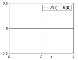
Refer to caption
Refer to caption
Refer to caption
Refer to caption
Refer to caption
Refer to caption
Refer to caption
Refer to caption
Refer to caption
Figure 1: Time evolution of the quantity 1R(t)1𝑅𝑡1-R(t) (left), the center of mass xcj(t)superscriptsubscript𝑥𝑐𝑗𝑡x_{c}^{j}(t) (middle), and the component mass ψj2superscriptnormsubscript𝜓𝑗2\|\psi_{j}\|^{2} and the total energy (t)𝑡\mathcal{E}(t) (right) for Case 1 in Example 4.9 for \textcolorblackκ=0,2,20𝜅0220\kappa=0,2,20 (top to bottom).

(a) (b) (c) (d)

Refer to caption
Refer to caption
Refer to caption
Refer to caption
Refer to caption
Refer to caption
Refer to caption
Refer to caption
Refer to caption
Refer to caption
Refer to caption
Refer to caption
Figure 2: Time evolution of the quantity 1R(t)1𝑅𝑡1-R(t) (left), the center of mass xcj(t)superscriptsubscript𝑥𝑐𝑗𝑡x_{c}^{j}(t) (middle), and the component mass ψj2superscriptnormsubscript𝜓𝑗2\|\psi_{j}\|^{2} and the total energy (t)𝑡\mathcal{E}(t) (right) for Case 2 in Example 4.9 for \textcolorblackκ=0,2,10,20𝜅021020\kappa=0,2,10,20 (top to bottom).
Example 4.10.

Here, we consider the six-component system in 2D, i.e., we take N=6𝑁6N=6 and d=2𝑑2d=2 in (2). To this end, we here only consider the identical case, i.e., we choose αj=1=βj=1subscript𝛼𝑗1subscript𝛽𝑗1\alpha_{j}=1=\beta_{j\ell}=1 (j,=1,,6formulae-sequence𝑗16j,\ell=1,\cdots,6 ). Let \textcolorblackκ=20𝜅20\kappa=20, we consider four cases of initial setups:

  • Case 3. x0j=(6cos((j1)π/3),6sin((j1)π/3))superscriptsubscript𝑥0𝑗6𝑗1𝜋36𝑗1𝜋3x_{0}^{j}=\big{(}6\,\cos((j-1)\pi/3),6\,\sin((j-1)\pi/3)\big{)},  j=1,,6𝑗16j=1,\cdots,6.

  • Case 4. x0j=(2+4cos(jπ/3π/12),2+4sin(jπ/3π/12))superscriptsubscript𝑥0𝑗24𝑗𝜋3𝜋1224𝑗𝜋3𝜋12x_{0}^{j}=\big{(}2+4\,\cos(j\pi/3-\pi/12),2+4\,\sin(j\pi/3-\pi/12)\big{)},  j=1,,6𝑗16j=1,\cdots,6.

  • Case 5. x0j=(6cos((j1)π/5),6sin((j1)π/5))superscriptsubscript𝑥0𝑗6𝑗1𝜋56𝑗1𝜋5x_{0}^{j}=\big{(}6\,\cos((j-1)\pi/5),6\,\sin((j-1)\pi/5)\big{)},  j=1,,6𝑗16j=1,\cdots,6.

  • Case 6. Random location:

    x01=(3.4707,2.7526),x02=(0.8931,1.9951),formulae-sequencesuperscriptsubscript𝑥013.47072.7526superscriptsubscript𝑥020.89311.9951\displaystyle x_{0}^{1}=(3.4707,2.7526),\quad x_{0}^{2}=(-0.8931,1.9951),
    x03=(0.1809,1.1538),x04=(0.0937,5.8995),formulae-sequencesuperscriptsubscript𝑥030.18091.1538superscriptsubscript𝑥040.09375.8995\displaystyle x_{0}^{3}=(0.1809,-1.1538),\quad x_{0}^{4}=(0.0937,-5.8995),
    x05=(2.9235,2.4171),x06=(3.6423,4.3714).formulae-sequencesuperscriptsubscript𝑥052.92352.4171superscriptsubscript𝑥063.64234.3714\displaystyle x_{0}^{5}=(-2.9235,-2.4171),\quad x_{0}^{6}=(-3.6423,4.3714).
\textcolor

blackFor Case 3-Case 6, Figure 3 illustrates the trajectory and time evolution of the center of mass xcj(t)=:(xc1j(t),xc2j(t))x_{c}^{j}(t)=:(x_{c1}^{j}(t),\,x_{c2}^{j}(t)), Figure 4 depicts the time evolution of |1256(t)1256(0)|subscript1256𝑡subscript12560|\mathcal{R}_{1256}(t)-\mathcal{R}_{1256}(0)|, |2456(t)2456(0)|subscript2456𝑡subscript24560|\mathcal{R}_{2456}(t)-\mathcal{R}_{2456}(0)| and |3456(t)3456(0)|subscript3456𝑡subscript34560|\mathcal{R}_{3456}(t)-\mathcal{R}_{3456}(0)|, and Figure 5 shows the contour plots of |ψ1(x,t)|2superscriptsubscript𝜓1𝑥𝑡2|\psi_{1}(x,t)|^{2} at different times. From these figures and other numerical experiments not shown here for brevity, we can see the following observations.

(i). Complete state aggregation occurs for all cases.

(ii). All the center of mass xcj(t)superscriptsubscript𝑥𝑐𝑗𝑡x_{c}^{j}(t) (j=1,,6𝑗16j=1,\cdots,6) will converge to the same periodic function x¯c(t)subscript¯𝑥𝑐𝑡\bar{x}_{c}(t), which swings exactly along the line connecting the points (x¯c10,x¯c20superscriptsubscript¯𝑥𝑐10superscriptsubscript¯𝑥𝑐20-\bar{x}_{c1}^{0},-\bar{x}_{c2}^{0}) and (x¯c10,x¯c20superscriptsubscript¯𝑥𝑐10superscriptsubscript¯𝑥𝑐20\bar{x}_{c1}^{0},\bar{x}_{c2}^{0} which are defined as the average of the initial center of mass of the six oscillators:

(x¯c10,x¯c20):=(16j=16xc1j(0),16j=16xc2j(0)).assignsuperscriptsubscript¯𝑥𝑐10superscriptsubscript¯𝑥𝑐2016superscriptsubscript𝑗16subscriptsuperscript𝑥𝑗𝑐1016superscriptsubscript𝑗16subscriptsuperscript𝑥𝑗𝑐20\left(\bar{x}_{c1}^{0},\bar{x}_{c2}^{0}\right):=\left(\frac{1}{6}\sum_{j=1}^{6}x^{j}_{c1}(0),\frac{1}{6}\sum_{j=1}^{6}x^{j}_{c2}(0)\right).

Thus, when x¯c10=x¯c20=0superscriptsubscript¯𝑥𝑐10superscriptsubscript¯𝑥𝑐200\bar{x}_{c1}^{0}=\bar{x}_{c2}^{0}=0, the center of mass will stay steady at the origin (cf. Figure 3 (a)), which also agrees with the conclusion in Remark 4.2 of [11].

\textcolor

black(iii) Before complete state aggregation, all density profiles |ψj(x,t)|2superscriptsubscript𝜓𝑗𝑥𝑡2|\psi_{j}(x,t)|^{2} (j=1,,6𝑗16j=1,\cdots,6) will evolve similarly, i.e., the same dynamical pattern as those shown in Figure 5 for |ψ1|2superscriptsubscript𝜓12|\psi_{1}|^{2} (only differ from the ‘color’, i.e., the more blurred humps imply the centers of the other five component, while the lighter one shows the one of the current component). While after complete state aggregation (around t=0.4𝑡0.4t=0.4, which corresponds to the moment the center of mass xcjsuperscriptsubscript𝑥𝑐𝑗x_{c}^{j} (j=1,,6𝑗16j=1,\cdots,6) meet together in Figure 3), all ψj(x,t)subscript𝜓𝑗𝑥𝑡\psi_{j}(x,t) (hence also for all density profiles) will converge to the same function, whose density changes periodically in time (as shown in columns 4–6 in Figure 5, which also indicate the periodic dynamics for the center of mass that illustrated in Figure 3). In addition, before complete state aggregation, although numerical schemes cannot conserve the cross-ratio like quantities ijkl(t)(1i,j,k,l6)subscript𝑖𝑗𝑘𝑙𝑡formulae-sequence1𝑖𝑗𝑘𝑙6\mathcal{R}_{ijkl}(t)(1\leq i,j,k,l\leq 6) in discretized level, the difference of those quantities from their initial ones are still small (cf. Figure 4).

(a) (b) (c) (d)
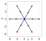
Refer to caption
Refer to caption
Refer to caption
Refer to caption
Refer to caption
Refer to caption
Refer to caption
Refer to caption
Refer to caption
Refer to caption
Refer to caption
Refer to caption
Figure 3: First two columns: trajectory of center of mass xcj(t)superscriptsubscript𝑥𝑐𝑗𝑡x_{c}^{j}(t) in t[0,tc]𝑡0subscript𝑡𝑐t\in[0,t_{c}] and t[tc,10]𝑡subscript𝑡𝑐10t\in[t_{c},10] (tc=1.5subscript𝑡𝑐1.5t_{c}=1.5 for first row while 0.5 for the others). The third column: time evolution of xc1j(t)superscriptsubscript𝑥𝑐1𝑗𝑡x_{c1}^{j}(t) and xc2j(t))x_{c2}^{j}(t)) (right). \circ denotes location of xcj(0)superscriptsubscript𝑥𝑐𝑗0x_{c}^{j}(0), while \Diamond denotes the one of xcj(tc)superscriptsubscript𝑥𝑐𝑗subscript𝑡𝑐x_{c}^{j}(t_{c}).
Refer to caption
Refer to caption
Refer to caption
Refer to caption
Figure 4: Time evolution of |1256(t)1256(0)|subscript1256𝑡subscript12560|\mathcal{R}_{1256}(t)-\mathcal{R}_{1256}(0)|, |2456(t)2456(0)|subscript2456𝑡subscript24560|\mathcal{R}_{2456}(t)-\mathcal{R}_{2456}(0)| and |3456(t)3456(0)|subscript3456𝑡subscript34560|\mathcal{R}_{3456}(t)-\mathcal{R}_{3456}(0)| for Case 3-6 (Left to right).

(a) (b) (c) (d)
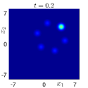
Refer to caption
Refer to caption
Refer to caption
Refer to caption
Refer to caption
Refer to caption
Refer to caption
Refer to caption
Refer to caption
Refer to caption
Refer to caption
Refer to caption
Refer to caption
Refer to caption
Refer to caption
Refer to caption
Refer to caption
Refer to caption
Refer to caption
Refer to caption
Refer to caption
Refer to caption
Refer to caption
Refer to caption
Refer to caption
Refer to caption
Figure 5: Contour plots of \textcolorblack|ψ1(x,t)|2superscriptsubscript𝜓1𝑥𝑡2|\psi_{1}(x,t)|^{2} at different time t𝑡t for Cases 3-5 in Example 4.10 (the top 4 rows) and color bars of the contour plots at t=0.5𝑡0.5t=0.5 (bottom left) and other time t𝑡t (bottom right).

5 Conclusion

In this survey paper, we have reviewed state-of-the-art results on the collective behaviors for two Lohe type aggregation models (the Lohe tensor model and the Schrödinger-Lohe model). The former deals with the aggregation dynamics of tensors with the same rank and size, and it turns out to be a generalized model for previously known first-order aggregation models such as the Kuramoto model, the swarm sphere model and the Lohe matrix model. Of course, the Lohe tensor model can be reduced to aggregation models on the hermitian sphere and nonsquare matrix group which are not known in previous literature. For the collective dynamics, we adopt two concepts of aggregation (complete state aggregation and practical aggregation). When all state aggregates to the same state, we call it as complete state aggregation. This phenomenon occurs for a homogeneous ensemble in which all particles follow the same free flow. In contrast, when states are governed by different free flows, complete state aggregation cannot occur. Of course, the rate of state change (we call it velocity) can aggregate to the same value. At present, this strong estimate is not available for the aforementioned models yet.

The latter describes the collective aggregation of the coupled Schrödinger equations for wave functions. For a special case, it can be reduced to the swarm sphere and Kuramoto models. For this model, we can also adopt the same universal approaches (Lyapunov functional approach and dynamical systems theory approach for two-point correlation functions). Similar to the Lohe tensor model, this model exhibits the same aggregation phenomena for homogeneous and heterogeneous ensembles. As we have already mentioned, we do not have a complete theory for dealing with a heterogeneous ensemble except for a weak aggregation estimate (practical aggregation). Thus, we would say that our reviewed results for a heterogeneous ensemble are still far from completeness. This will be an interesting research direction for those who are interested in collective dynamics.

Acknowledgments

The content of this paper is based on a lecture given by the first author at the Institute of Mathematical Sciences of National University of Singapore in December 2019. The authors acknowledge the Institute of Mathematical Sciences for generous support and especially thank Prof. Weizhu Bao for the invitation and his warm hospitality. The work of S.-Y. Ha is supported by the NRF grant (2020R1A2C3A01003881) and the work of D. Kim was supported by the National Research Foundation of Korea (NRF) grant funded by the Korea government (MSIT) (No.2021R1F1A1055929).

References

  • [1] J. A. Acebron, L. L. Bonilla, C. J. P. Pérez Vicente, F. Ritort and R. Spigler, “The Kuramoto model: a simple paradigm for synchronization phenomena’,’ Rev. Mod. Phys., 77 (2005), 137–185.
  • [2] G. Albi, N. Bellomo, L. Fermo, S.-Y. Ha, J. Kim, L. Pareschi, D. Poyato and J. Soler, “Vehicular traffic, crowds and swarms: From kinetic theory and multiscale methods to applications and research perspectives.”, Math. Models Methods Appl. Sci., 29 (2019), 1901–2005.
  • [3] X. Antoine and R. Duboscq, “ Robust and efficient preconditioned Krylov spectral solvers for computing the ground states of fast rotating and strongly interacting Bose-Einstein condensates”, J. Comput. Phys., 258 (2014), 509–523.
  • [4] P. Antonelli and P. Marcati, “A model of synchronization over quantum networks”, J. Phys. A., 50 (2017), 315101.
  • [5] W. Bao, “Ground states and dynamics of multicomponent Bose-Einstein condensates”, Multiscale Model. SImul., 2 (2004), 210–236.
  • [6] W. Bao and Y. Cai,“Mathematical models and numerical methods for spinor Bose-Einstein condensates”, Commun. Comput. Phys., 24 (2018), 899–965.
  • [7] W. Bao and Y. Cai, “Mathematical theory and numerical methods for Bose-Einstein condensation”, Kinet. Relat. Models, 6 (2013), 1–135.
  • [8] W. Bao and Y. Cai, “Uniform error estimates of finite difference methods for the nonlinear Schrödinger equation with wave operator”, SIAM J. Numer. Anal., 50 (2012), 492–521.
  • [9] W. Bao, I. Chern and F. Lim, “Efficient and spectrally accurate numerical methods for computing ground and first excited states in Bose-Einstein condensates”, J. Comput. Phys., 219 (2006), 836–854.
  • [10] W. Bao, D. Jaksch and P. A. Markowich, “Numerical solution of the Gross-Pitaevskii equation for Bose-Einstein condensation”, J. Comput. Phys., 187 (2003), 318–342.
  • [11] W. Bao, S.-Y. Ha, D. Kim and Q. Tang, “Collective synchronization of the multi-component Gross-Pitaevskii-Lohe system”, Phys. D, 400 (2019), 132158.
  • [12] J. Bronski, T. Carty and S. Simpson, “A matrix valued Kuramoto model”, J. Stat. Phys., 178 (2020), 595–624.
  • [13] J. Buck and E. Buck, “Biology of synchronous flashing of fireflies”, Nature, 211 (1966), 562–564.
  • [14] J. Byeon, S.-Y. Ha, G. Hwang and H. Park, “Emergent behaviors of the kinetic Lohe Hermitian sphere model”, Archived as arXiv:2104.13036.
  • [15] J. Byeon, S.-Y. Ha, and H. Park, “Asymptotic interplay of states and adapted coupling gains in the Lohe hermitian sphere model”, Archived as arXiv:2101.03450.
  • [16] J. A. Carrillo, Y.-P. Choi, C. Totzeck and O. Tse, “An analytical framework for consensus-based global optimization method”, Math. Models Methods Appl. Sci., 28 (2018), 1037–1066.
  • [17] J. A. Carrillo, S. Jin, L. Li and Y. Zhu, “A consensus-based global optimization method for high dimensional machine learning problems”, ESAIM: COCV, 27 (2021), S5.
  • [18] D. Chi, S.-H. Choi and S.-Y. Ha, “Emergent behaviors of a holonomic particle system on a sphere”, J. Math. Phys., 55 (2014), 052703.
  • [19] J. Cho, S.-H. Choi and S.-Y. Ha, “Practical quantum synchronization for the Schrödinger-Lohe system”, J. Phys. A, 49 (2016), 205203.
  • [20] S.-H. Choi and S.-Y. Ha, “Time-delayed interactions and synchronization of identical Lohe oscillators”, Quart. Appl. Math., 74 (2016), 297==319.
  • [21] S.-H. Choi and S.-Y. Ha, “Large-time dynamics of the asymptotic Lohe model with a small time-delay”, J. Phys. A., 48 (2015), 425101.
  • [22] S.-H. Choi and S.-Y. Ha, “Quantum synchronization of the Schrödinger-Lohe model”, J. Phys. A, 47 (2014), 355104.
  • [23] S.-H. Choi and S.-Y. Ha, “Complete entrainment of Lohe oscillators under attractive and repulsive couplings”, SIAM J. Appl. Dyn. Syst., 13 (2014), 1417–1441.
  • [24] F. Cucker and S. Smale, “Emergent behavior in flocks”, IEEE Trans. Automat. Control, 52 (2007), 852–862.
  • [25] P. Degond, A. Frouvelle, S. Merino-Aceituno and A. Trescases, “Quaternions in collective dynamics”, Multiscale Model. Simul., 16 (2018), 28–77.
  • [26] L. DeVille, “Synchronization and stability for quantum Kuramoto”, J. Stat. Phys., 174 (2019), 160–187.
  • [27] F. Dörfler and F. Bullo, “Synchronization in complex networks of phase oscillators: A survey”, Automatica, 50 (2014), 1539–1564.
  • [28] M. Fornasier, H. Huang, L. Pareschi and P. Sunnen, “Consensus-based optimization on the sphere II: Convergence to global minimizers and machine learning.” Archived as arXiv:2001.11988.
  • [29] Fornasier, M., Huang, H., Pareschi, L. and Sunnen, P.:Consensus-based optimization on hypersurfaces: Well-posedness and mean-field limit. Math. Models Methods Appl. Sci. 30 (2020), 2725–2751.
  • [30] F. Golse, and S.-Y. Ha, “A mean-field limit of the Lohe matrix model and emergent dynamics.” Arch. Rational Mech. Anal., 234 (2019), 1445–1491.
  • [31] S.-Y. Ha, G. Hwang, and D. Kim, “Remarks on the stability properties for the continuous and discrete Schrödinger-Lohe system”, In preparation.
  • [32] S.-Y. Ha, G. Hwang and H. Park, “Emergent behaviors of Lohe Hermitian sphere particles under time-delay interactions”, Netw. Heterog Media, (2021).
  • [33] S.-Y. Ha, M. Kang and H. Park, “Collective behaviors of the Lohe Hermitian sphere model with inertia”, Commun. Pure Appl. Anal., (2021).
  • [34] S.-Y. Ha, M. Kang and H. Park, “Emergent dynamics of the Lohe Hermitian sphere model with frustration”, J. Math. Phys., 62 (2021), 052701.
  • [35] S.-Y. Ha and D. Kim, “Emergence of synchronous behaviors for the Schrödinger-Lohe model with frustration”, Nonlinearity, 32 (2019), 4609–4637.
  • [36] S.-Y. Ha and D. Kim, “Uniform stability and emergent dynamics of particle and kinetic Lohe matrix models”, Under review.
  • [37] S.-Y. Ha, D. Kim, J. Lee and S. E. No, “Particle and kinetic models for swarming particles on a sphere and stability properties”, J. Stat. Phys., 174 (2019), 622–655.
  • [38] S.-Y. Ha, D. Kim and H. Park, “Existence and emergent dynamics of quadratically separable states to the Lohe tensor model”, Archived as arXiv:2103.17029.
  • [39] S.-Y. Ha, D. Kim and H. Park, “On the completely separable state for the Lohe tensor model”, J. Stat. Phys., 183 (2021).
  • [40] S.-Y. Ha, D. Ko, J. Park and X. Zhang, “Collective synchronization of classical and quantum oscillators”, EMS Surv. Math. Sci., 3 (2016), 209–267.
  • [41] S.-Y. Ha and H. Park, “A gradient flow formulation of the Lohe matrix model with a high-order polynomial coupling”, To appear in J. Stat. Phys.
  • [42] S.-Y. Ha and H. Park, “Emergent behaviors of the generalized Lohe matrix model”, Discrete Contin. Dyn. Syst. B, 26 (2021), 4227–4261.
  • [43] S.-Y. Ha and H. Park, “Complete aggregation of the Lohe tensor model with the same free flow”, J. Math. Phys., 61 (2020), 102702.
  • [44] S.-Y. Ha and H. Park, ”From the Lohe tensor model to the Lohe Hermitian sphere model and emergent dynamics”, SIAM J. Appl. Dyn. Syst., 19 (2020), 1312–1342.
  • [45] S.-Y. Ha and H. Park, “Emergent behaviors of Lohe tensor flock”, J. Stat. Phys., 178 (2020), 1268–1292.
  • [46] S.-Y. Ha and S. W. Ryoo, “On the emergence and orbital Stability of phase-locked states for the Lohe model”, J. Stat. Phys., 163 (2016), 411–439.
  • [47] H. Huh and S.-Y. Ha, “Dynamical system approach to synchronization of the coupled Schrödinger–Lohe system”, Quart. Appl. Math., 75 (2017), 555–579.
  • [48] H. Huh, S.-Y. Ha and D. Kim, “Emergent behaviors of the Schrödinger-Lohe model on cooperative-competitive network”, J. Differential Equations, 263 (2017), 8295–8321.
  • [49] H. Huh, S.-Y. Ha and D. Kim, “Asymptotic behavior and stability for the Schrödinger-Lohe model”, J. Math. Phys., 59 (2018), 102701.
  • [50] V. Jaćimović and A. Crnkić, “Low-dimensional dynamics in non-Abelian Kuramoto model on the 3-sphere”, Chaos, 28 (2018), 083105.
  • [51] T. Kanamori and A. Takeda, “Non-convex optimization on Stiefel manifold and applications to machine learning”, International Conference on Neural Information Processing, Springer, 2012, 109–116.
  • [52] J. Kennedy and R. Eberhart, “Particle swarm optimization”, Proceedings of ICNN’95-International Conference on Neural Networks, vol. 4, IEEE, 1995, 1942–1948.
  • [53] Y. Kuramoto, Self-entrainment of a population of coupled non-linear oscillators, In International Symposium on Mathematical Problems in Mathematical Physics. Lecture Notes in Theoretical Physics 30 (1975), 420–422.
  • [54] N. E. Leonard, D. A. Paley, F. Lekien, R. Sepulchre, D. M. Fratantoni and R. E. Davis,“Collective motion, sensor networks and ocean sampling”, Proc. IEEE, 95 (2007), 48-74.
  • [55] M. A. Lohe, “On the double sphere model of synchronization”, Phys. D., 412 (2020), 132642.
  • [56] M. A. Lohe, “Quantum synchronization over quantum networks”, J. Phys. A, 43 (2010), 465301.
  • [57] M. A. Lohe, “Non-Abelian Kuramoto model and synchronization”, J. Phys. A, 42 (2009), 395101.
  • [58] J. Markdahl, J. Thunberg and J. Gonçalves, “Almost global consensus on the n-sphere”, IEEE Trans. Automat. Control, 63 (2018), 1664–1675.
  • [59] R. Olfati-Saber,“Swarms on sphere: A programmable swarm with synchronous behaviors like oscillator network”, Proc. of the 45th IEEE conference on Decision and Control, (2006), 5060–5066.
  • [60] S. Motsch and E. Tadmor, “Heterophilious dynamics enhances consensus”, SIAM. Rev., 56 (2014), 577–621.
  • [61] D. A. Paley, N. E. Leonard, R. Sepulchre, D. Grunbaum and J. K. Parrish, “Oscillator models and collective motion”, IEEE Contr. Syst. Mag., 27 (2007), 89–105.
  • [62] C. S. Peskin, Mathematical Aspects of Heart Physiology, Courant Institute of Mathematical Sciences, New York, 1975.
  • [63] A. Pikovsky, M. Rosenblum and J. Kurths, Synchronization: A universal concept in nonlinear sciences. Cambridge University Press, Cambridge, 2001.
  • [64] R. Pinnau, C. Totzeck, O. Tse and S. Martin, “A consensus-based model for global optimization and its mean-field limit”, Math. Models Methods Appl. Sci., 27 (2017), 183–204.
  • [65] C. W. Reynolds, “Flocks, herds and schools: A distributed behavioral model”, Proceeding SIGGRAPH 87 Proceedings of the 14th annual conference on Computer graphics and interactive techniques, (1987), 25–34.
  • [66] S. H. Strogatz, “From Kuramoto to Crawford: Exploring the onset of synchronization in populations of coupled oscillators”, Phys. D, 143 (2000), 1–20.
  • [67] J. Thunberg, J. Markdahl, F. Bernard and J. Goncalves, “A lifting method for analyzing distributed synchronization on the unit sphere”, Automatica, 96 (2018), 253–258.
  • [68] C. M. Topaz, A. L. Bertozzi and M. A. Lewis, “A nonlocal continuum model for biological aggregation”, Bull. Math. Biol., 68 (2006), 1601–1623.
  • [69] C. M. Topaz and A. L. Bertozzi, “Swarming patterns in a two-dimensional kinematic model for biological groups”, SIAM J. Appl. Math., 65 (2004), 152–174.
  • [70] T. Vicsek, A. Czirók, E. Ben-Jacob, I. Cohen and O. Shochet, “Novel type of phase transition in a system of self-driven particles”, Phys. Rev. Lett., 75 (1995), 1226–1229.
  • [71] T. Vicsek and A. Zefeiris, “Collective motion”, Phys. Rep., 517 (2012), 71–140.
  • [72] A. T. Winfree, The geometry of biological time. Springer, New York, 1980.
  • [73] A. T. Winfree, “Biological rhythms and the behavior of populations of coupled oscillators”, J. Theor. Biol., 16 (1967), 15–42.
  • [74] J. Zhu,“Synchronization of Kuramoto model in a high-dimensional linear space”, Phys. Lett. A, 377 (2013), 2939–2943.