Exclusive Group Lasso for Structured Variable Selection

Abstract

A structured variable selection problem is considered in which the covariates, divided into predefined groups, activate according to sparse patterns with few nonzero entries per group. Capitalizing on the concept of atomic norm, a composite norm can be properly designed to promote such exclusive group sparsity patterns. The resulting norm lends itself to efficient and flexible regularized optimization algorithms for support recovery, like the proximal algorithm. Moreover, an active set algorithm is proposed that builds the solution by successively including structure atoms into the estimated support. It is also shown that such an algorithm can be tailored to match more rigid structures than plain exclusive group sparsity. Asymptotic consistency analysis (with both the number of parameters as well as the number of groups growing with the observation size) establishes the effectiveness of the proposed solution in terms of signed support recovery under conventional assumptions. Finally, a set of numerical simulations further corroborates the results.

Keywords: Structured sparsity, exclusive group Lasso, proximal, active set, asymptotic consistency.

1 Introduction

The problem of estimating a sparse signal that has some known structural properties has arisen a lot of interest in statistical inference over the past decade. The problem was originally focused on recovering certain data or signal by exploiting a given parsimonious representation that describes it Candès et al. (2006); Donoho (2006). The underlying idea is that the observation can be modeled as a sparse linear combination of the columns of a certain measurement matrix, a fact that can be exploited in order to retrieve the signal with a number of measurements that is essentially commensurate with the sparsity level of the model rather than the number of free parameters.

This basic sparse representation can be generalized to include more elaborate descriptions of the data, which have traditionally been referred to as structured sparsity. According to these models, the observation can be described as a linear combination of very few columns of a measurement matrix, where the activation of a certain covariate is inherently coupled with the activation of some additional ones. The most relevant example of this type of inherent signal structure is strong group sparsity Huang and Zhang (2010), where groups of covariates are simultaneously activated in the underlying linear model.

Recently, there has been an increased interest in other types of sparsity structure which have been shown to be a more accurate description of data in real applications. This is the case of exclusive group sparsity, which accounts for the fact that the covariates in the underlying model can be collected in groups, so that only few covariates per group are in practice activated. This type of structure is more general than conventional strong group sparsity and therefore more difficult to exploit. Note, in fact, that exclusive group sparsity becomes conventional group sparsity when the activation of a certain covariate in a group is linked to the activation of some fixed covariates in the other ones. This higher degree of abstraction of exclusive group sparsity models has recently spurred its application in a number of fields, as diverse as multi-label image classification Chen et al. (2011), object tracking Zhang et al. (2016), behavioral research Kok et al. (2019), parallel acquisition Chun and Adcock (2017), MIMO radar Dorsch and Rauhut (2017), gene selection or nuclear magnetic resonance spectroscopy Campbell and Allen (2017).

In the recent literature, exclusive group sparsity has also been referred to as “sparsity in levels” Adcock et al. (2017). Lately, there has been considerable interest in the link between exclusive group sparsity and multi-level sampling methods based on isometries. In particular, Adcock et al. (2017) provided some non-uniform recovery guarantees of exclusive group sparse signals by $\ell_{1}$ norm minimization in combination with multi-label sampling of an isometry measurement matrix. Later, in Li and Adcock (2019) and Bastounis and Hansen (2017) these recovery bounds were generalized to uniform guarantees by imposing a certain restricted isometry property in levels of the underlying matrix.

Additional efforts have recently been focused on improved recovery methods for exclusive group sparsity problems. In particular, several recent works have focused on the use of optimization penalties that mimic the effect of classical Lasso Tibshirani (1996) and group Lasso Yuan and Lin (2006) regularizers. The equivalent problem in exclusive group sparsity models is usually referred to as exclusive Lasso, and consists of a penalty first introduced in Zhou et al. (2010) in the context of multi-task feature selection. This regularizer is in fact a composite norm, where the $\ell_{1}$ norm is applied group-wise, the outcome of which is then combined according to a conventional $\ell_{2}$ norm. In this sense, the exclusive group Lasso penalty can be seen as a direct transposition of conventional group Lasso, where the $\ell_{2}$ norm is applied to the different columns, which are then combined according to an $\ell_{1}$ paradigm. In exclusive group Lasso these norms are applied in reverse order.

One of the most extensive studies of the exclusive group sparse regularizer was presented in Campbell and Allen (2017). This paper considered this type of regularization in linear regression problems and studied the statistical consistency properties of the associated estimators. The fact that the exclusive Lasso penalty is not continuously differentiable (due to the presence of the $\ell_{1}$ norm at the group level) has motivated the study of optimized solutions to the associated optimization problem. For example, Campbell and Allen (2017) proposed a coordinate descent method, whereas Kong et al. (2014) and Yamada et al. (2017) considered the use of iteratively re-weighted algorithms to solve the penalized problem. Recently, Lin et al. (2019) proposed a dual Newton based preconditioned proximal point algorithm for a weighted version of the exclusive Lasso.

It should be stressed here that the exclusive group sparse regularizer can be seen as a special case of more general mixed norm regularizers, where the $\ell_{p}$ norm is applied at the group level and the $\ell_{q}$ norm is used to combine the result. Kowalski (2009) considered the use of these general mixed norm regularizers in regression problems and provided an expression for the proximal of the square of the weighted exclusive sparsity norm, which was then used as the basis of a thresholded Landweber algorithm. This can be used to formulate direct proximal gradient methods for the exclusive group Lasso, see also Lin et al. (2019).

The objective of this paper is to study the application of exclusive group sparse penalty in order to promote certain sparsity structures beyond covariance exclusivity. To that effect, we will propose an active set algorithm based on the use of exclusive Lasso for agglomerative activation of covariates according to some promoted sparsity structure. We will also extend the work in Campbell and Allen (2017) by establishing sharp recovery bounds for signed support recovery. To that effect we will consider the signal recovery via linear regression with exclusive sparsity norm penalization and follow the approach originally established in Wainwright (2009).

The rest of the paper is organized as follows. Section 2 introduces the exclusive group sparsity norm from the mathematical perspective and compares it with some other penalties in the literature that promote structured sparsity. Section 3 presents some useful properties of the exclusive group sparsity norm that will be used throughout the paper. For minimization problems that include the exclusive group sparsity norm as a regularizer, Section 4 proposes an efficient solving algorithm based on the proximal operator. Section 5 introduces an active set algorithm that is able to promote some sparsity structures along a certain evolution path. Section 6 studies the conditions that guarantee signed support consistency of the corresponding exclusive Lasso algorithm. Section 7 provides a comparative numerical assessment of the proposed algorithm and finally Section 8 concludes the paper. Most of the technical proofs can be found in the Appendix.

2 Exclusive group sparsity formulation

Our objective is the recovery of a certain $p$-dimensional column vector $\mathbf{x}$ that presents an exclusive group sparsity structure. The entries of $\mathbf{x}$ will indistinctively be referred to as covariates, variables or entries, and will be denoted as $x_{i}$, $i\in[p]$, where $[p]=\{1,\ldots,p\}$. We will define the support of $\mathbf{x}$ as $\mathcal{J}=\operatorname{supp}\{\mathbf{x}\}=\{i\in[p]:x_{i}\neq 0\}$. The complementary of the support will be written as $\mathcal{J}^{\mathrm{c}}=[p]\backslash\mathcal{J}$.

Let us consider a general partition $\mathcal{G}$ of the set of indices $[p]=\{1,2,\dots,p\}$, that is $\bigcup_{G\in\mathcal{G}}G=[p]$ and $G\cap G^{\prime}=\emptyset$ for all $G,G^{\prime}\in\mathcal{G},G\neq G^{\prime}$. For any $\mathbf{x}\in\mathbb{R}^{p}$, $p\in\mathbb{N}$, the exclusive group sparsity norm is defined as

$$\Omega_{\mathrm{excl}}(\mathbf{x})=\sqrt{\sum_{G\in\mathcal{G}}\lVert\mathbf{x}_{G}\rVert_{1}^{2}}$$ (1)

where $\lVert\cdot\rVert_{1}$ denotes the $\ell_{1}$ norm and where $\mathbf{x}_{G}$ is a $|G|$-dimensional subvector of $\mathbf{x}$ with entries indexed by $G$. Observe that, as explained above, this definition corresponds to a composite norm, where the $\ell_{1}$ norm is applied at the group level ($\lVert\mathbf{x}_{G}\rVert_{1}$, $G\in\mathcal{G}$) whereas the $\ell_{2}$ norm combines the contributions from the different groups. The conventional group sparsity norm follows the same approach and can simply be recovered by interchanging the order in which these two norms are applied.

Remark 1

In some parts of the paper, we will need to build a $p$-dimensional vector with all zero entries except for those indexed by $G\in\mathcal{G}$, which correspond to $\mathbf{x}_{G}$. We will denote this $p$-dimensional vector as $\mathbf{x}_{\{G\}}$.

The objective of this paper is to explore the properties of norm $\Omega_{\mathrm{excl}}(\mathbf{x})$ and to derive some efficient algorithms to tackle optimization problems where $\Omega_{\mathrm{excl}}(\mathbf{x})$ regularizes the solution in favor of a characteristic sparsity pattern. Specifically, we are interested in solution vectors where the active entries are evenly distributed among the groups of partition $\mathcal{G}$ while promoting the selection of a sparse number of variables within each group (hence the name exclusive group sparsity).

The exclusive group sparsity structure enforced by $\Omega_{\mathrm{excl}}(\mathbf{x})$ becomes apparent once noticing that our norm is the composition between the $\ell_{1}$ norm (within each group) and the $\ell_{2}$ norm (among groups). This composite norm can also be seen as the atomic norm (see Chandrasekaran et al. (2010)) induced by the set of atoms

$$\mathcal{A}=\Bigl{\{}\mathbf{a}\in\mathbb{R}^{p}:\mathbf{a}_{G}=\alpha_{G}\mathbf{e}_{i}^{\lvert G\rvert},\quad i\in[\lvert G\rvert],\quad\alpha_{G}\in\mathbb{R},\quad\forall G\in\mathcal{G},\quad\text{s.to }\sum_{G\in\mathcal{G}}\alpha_{G}^{2}=1\Bigr{\}}$$

where $\{\mathbf{e}_{i}^{\lvert G\rvert}\}_{i=1,2,\dots,\lvert G\rvert}$ denotes the canonical basis of $\mathbb{R}^{\lvert G\rvert}$. More formally,

$$\Omega_{\mathrm{excl}}(\mathbf{x})=\inf\Biggl{\{}\sum_{\mathbf{a}\in\mathcal{A}}c_{\mathbf{a}}:\mathbf{x}=\sum_{\mathbf{a}\in\mathcal{A}}c_{\mathbf{a}}\mathbf{a},\quad c_{\mathbf{a}}\geq 0\Biggr{\}}.$$ (2)

Here, we focus on practical aspects that arise when facing the regularized optimization problems

$$\operatorname*{minimize\,}_{\mathbf{x}\in\mathbb{R}^{p}}L(\mathbf{x})+\lambda\Omega_{\mathrm{excl}}(\mathbf{x})\quad\text{or}\quad\operatorname*{minimize\,}_{\mathbf{x}\in\mathbb{R}^{p}}L(\mathbf{x})+\frac{\mu}{2}\Omega_{\mathrm{excl}}^{2}(\mathbf{x})$$ (3)

where $L:\mathbb{R}^{p}\to\mathbb{R}_{+}$ is a convex and continuously differentiable loss function. It is worth recalling that the two problems above can always be made equivalent by properly choosing the values of the two regularization parameters $\lambda,\mu\in\mathbb{R}_{+}$, see Bach et al. (2012).

2.1 Other approaches to structured sparsity

A noticeable duality exists between the norm in (1) and the group-Lasso penalty $\sum_{G\in\mathcal{G}}\lVert\mathbf{x}_{G}\rVert_{2}$, which also consists in the composition of the $\ell_{1}$ and $\ell_{2}$ norms but in the opposite order to $\Omega_{\mathrm{excl}}(\mathbf{x})$ (see, e.g., Yuan and Lin (2006)). As one may expect, the effect is profoundly different: In the group-Lasso penalty, the group is the structural atom and, as such, all its elements are either active or set to zero (Huang et al. (2011)). Conversely, as we will prove in the next sections, penalty $\Omega_{\mathrm{excl}}(\mathbf{x})$ ensures that all groups are active and contain a comparable number of nonzero regression coefficients.

Obozinski et al. (2011) extends the group-Lasso approach by applying the $\ell_{1}/\ell_{2}$ norm to groups that may overlap (that is, they do not form a partition of $[p]$ any more, even though all entries of $\mathbf{x}$ belong to at least one group). Their approach is similar to the one developed here, in the sense that both approaches can be formulated as a minimum-weight atomic representation analogous to the Minkowski functional. Specifically, let $\mathcal{H}$ denote the family of overlapping groups and $\mathbf{a}_{H}$ be the generic vector supported by $H\in\mathcal{H}$ (the latent vectors in the nomenclature of that paper). Then, the latent group Lasso penalty is defined as

$$\Omega_{\textrm{latent}}(\mathbf{x})=\inf_{\{\mathbf{a}_{H},c_{H}\}_{H\in\mathcal{H}}}\Biggl{\{}\sum_{H\in\mathcal{H}}c_{H}:\mathbf{x}=\sum_{H\in\mathcal{H}}c_{H}\mathbf{a}_{H},\quad c_{H}\geq 0,\quad\lVert\mathbf{a}_{H}\rVert_{2}=d_{H}^{-1}\Biggr{\}}.$$ (4)

where $d_{H}>0$ is a fixed weight assigned to group $H\in\mathcal{H}$. The benefit of latent group Lasso over classic group Lasso is the possibility to consider sparsity patterns with more flexible structure than well-localized groups of correlated covariates.

Interestingly enough, the affinity between the latent group Lasso and our penalty (1) is not limited to the underlying atomic formulation. Indeed, it is sometimes possible to define the families of groups $\mathcal{G}$, associated to the exclusive group sparse penalty, and $\mathcal{H}$, for the latent group Lasso, so that the induced sparsity structures are almost equivalent. For instance, in (Obozinski et al., 2011, Section 6.3), it is shown that the latent group Lasso norm in the case $p=4$ and $\mathcal{H}=\{\{1,2\},\{1,3\},\{2,4\},\{3,4\}\}$ is equivalent to the exclusive group sparsity norm with groups $\mathcal{G}=\{\{1,4\},\{2,3\}\}$, namely

$$\Omega_{\textrm{latent}}(\mathbf{x})=\Omega_{\mathrm{excl}}(\mathbf{x})=\sqrt{(\lvert x_{1}\rvert+\lvert x_{4}\rvert)^{2}+(\lvert x_{2}\rvert+\lvert x_{3}\rvert)^{2}}.$$

Even if it is usually not possible to draw an exact equivalence between the two norms as in this example, one can sometimes map the latent groups $\mathcal{H}$ into a family $\mathcal{G}$ that induces a similar, though slightly relaxed, sparsity structure. It is worth noticing that, conversely to the exclusive group sparsity norm in (1), the latent group Lasso penalty usually lacks a closed-form expression.

Several other works deal with structured sparsity, although there is no direct correspondence between their models and ours (see, e.g., Shervashidze and Bach (2015); Rao et al. (2016); Bayram and Bulek (2017)). A special mention is deserved to Jenatton et al. (2011a), since it inspired the active set algorithm derived in Section 5. In that paper the focus is still on overlapping groups, with the considered norm being

$$\Omega_{\textrm{svs}}(\mathbf{x})=\sum_{H\in\mathcal{H}}\lVert\mathbf{d}_{H}\odot\mathbf{x}\rVert_{2}$$ (5)

where $\mathbf{d}_{H}$ is a vector supported by $H$ of positive weights and $\odot$ denotes the Hadamard element-wise product (and “svs” stands for structured variable selection). The main characteristic of the structured variable selection approach is that it induces a solution support that is the intersection of a subset of the groups contained in $\mathcal{H}$. Conversely, the latent group Lasso in (4) promotes solutions whose support is the union of a subset of groups in $\mathcal{H}$. The outcome of both approaches is fundamentally different from the support patterns that are favored by the exclusive group sparse penalty, which promotes the activation of very few elements within each group of $\mathcal{G}$, while guaranteeing that their contribution is evenly distributed across all groups. As we will see in Section 7, this fact has a significant impact on the support structures that can be detected.

3 Norm proprieties

In this section we provide some basic properties of norm $\Omega_{\mathrm{excl}}(\mathbf{x})$ which will be useful in the rest of the paper. Besides, they offer a different perspective for understanding the behavior of the norm as a regularizer and for grasping more insight into the promoted sparsity structure.

3.1 Dual norm and subdifferential

To begin with, we give a closed-form expression for the dual norm associated to $\Omega_{\mathrm{excl}}(\mathbf{x})$ that, by definition, is given by $\Omega_{\mathrm{excl}}^{*}(\mathbf{u})=\sup\{\mathbf{u}^{\mathrm{T}}\mathbf{x}:\mathbf{u}\in\mathbb{R}^{p},\Omega_{\mathrm{excl}}(\mathbf{x})\leq 1\}$. Routine computation shows that, for the norm in (1), the dual norm is

$$\Omega_{\mathrm{excl}}^{*}(\mathbf{u})=\sqrt{\sum_{G\in\mathcal{G}}\lVert\mathbf{x}_{G}\rVert_{\infty}^{2}}$$ (6)

where we recall that $\mathcal{G}$ is a partition of $[p]$.

Knowing the dual norm allows the following convenient characterization of the subdifferential of the norm, that is the set of all subgradients of $\Omega_{\mathrm{excl}}(\cdot)$ at $\mathbf{x}\in\mathbb{R}^{p}$ (see, e.g., (Bach et al., 2012, Remark 1.1)):

$$\partial\Omega_{\mathrm{excl}}(\mathbf{x}) =\{\mathbf{u}\in\mathbb{R}^{p}:\Omega_{\mathrm{excl}}(\mathbf{y})\geq\Omega_{\mathrm{excl}}(\mathbf{x})+\mathbf{u}^{\mathrm{T}}(\mathbf{y}-\mathbf{x}),\forall\mathbf{y}\in\mathbb{R}^{p}\}$$

$$=\{\mathbf{u}\in\mathbb{R}^{p}:\mathbf{u}^{\mathrm{T}}\mathbf{x}=\Omega_{\mathrm{excl}}(\mathbf{x})\text{ and }\Omega_{\mathrm{excl}}^{*}(\mathbf{u})\leq 1\}.$$ (7)

Indeed, the Fenchel–Young inequality states that, for $\mathbf{u},\mathbf{x}\in\mathbb{R}^{p}$, we have $\mathbf{x}^{\mathrm{T}}\mathbf{u}\leq\Omega_{\mathrm{excl}}(\mathbf{x})+\mathbb{I}_{\Omega_{\mathrm{excl}}^{\ast}(\mathbf{u})\leq 1}$, where $\mathbb{I}_{A}$ is the identity function associated to the event $A$ ($\mathbb{I}_{A}=0$ when $A$ is true and $\mathbb{I}_{A}=+\infty$ otherwise). Furthermore, strict equality holds if and only if $\mathbf{u}\in\partial\Omega_{\mathrm{excl}}(\mathbf{x})$. We can therefore identify the elements of $\partial\Omega_{\mathrm{excl}}(\mathbf{x})$ with the elements $\mathbf{u}\in\mathbb{R}^{p}$ for which Fenchel–Young holds with equality, that is (7).

The following characterization of the subdifferential will be helpful in deriving the results of the next sections.

Lemma 2

For all $\mathbf{x}\in\mathbb{R}^{p}\setminus\{\mathbf{0}\}$, $\mathbf{u}\in\partial\Omega_{\mathrm{excl}}(\mathbf{x})$ if and only if

$$\lvert u_{i}\rvert=\frac{\lVert\mathbf{x}_{G_{i}}\rVert_{1}}{\Omega_{\mathrm{excl}}(\mathbf{x})}\qquad\text{and}\qquad\operatorname{sign}(u_{i})=\operatorname{sign}(x_{i}) \forall i:x_{i}\neq 0$$

$$\hskip 85.35826pt\lvert u_{i}\rvert\leq\frac{\lVert\mathbf{x}_{G_{i}}\rVert_{1}}{\Omega_{\mathrm{excl}}(\mathbf{x})} \forall i:x_{i}=0$$

where $G_{i}$ is the (unique) group containing index $i$.

Proof  Sufficiency is direct once we observe that the conditions on $\lvert u_{i}\rvert$ imply that

$$\lVert\mathbf{u}_{G}\rVert_{\infty}=\frac{\lVert\mathbf{x}_{G}\rVert_{1}}{\Omega_{\mathrm{excl}}(\mathbf{x})}$$

for all $G\in\mathcal{G}$.

To prove necessity, we can proceed as follows. By (7) and the definition of dual norm, we have

$$\Omega_{\mathrm{excl}}(\mathbf{x})=\mathbf{u}^{\mathrm{T}}\mathbf{x}\leq\Omega_{\mathrm{excl}}(\mathbf{x})\Omega_{\mathrm{excl}}^{*}(\mathbf{u})\leq\Omega_{\mathrm{excl}}(\mathbf{x})$$

which implies that $\mathbf{u}\in\partial\Omega_{\mathrm{excl}}(\mathbf{x})$, $\mathbf{x}\neq\mathbf{0}$, if and only if equality holds everywhere. But,

$$\mathbf{u}^{\mathrm{T}}\mathbf{x}=\sum_{G\in\mathcal{G}}\mathbf{u}_{G}^{\mathrm{T}}\mathbf{x}_{G}\stackrel{{\scriptstyle\mathrm{(a)}}}{{\leq}}\sum_{G\in\mathcal{G}}\lVert\mathbf{u}_{G}\rVert_{\infty}\lVert\mathbf{x}_{G}\rVert_{1}\stackrel{{\scriptstyle\mathrm{(b)}}}{{\leq}}\sqrt{\sum_{G\in\mathcal{G}}\lVert\mathbf{u}_{G}\rVert_{\infty}^{2}}\sqrt{\sum_{G\in\mathcal{G}}\lVert\mathbf{x}_{G}\rVert_{1}^{2}}=\Omega_{\mathrm{excl}}(\mathbf{x})\Omega_{\mathrm{excl}}^{*}(\mathbf{u})$$

and, by the previous observation, equality must hold everywhere.

An equality in (a) implies that $\lvert u_{i}\rvert=\lVert\mathbf{u}_{G}\rVert_{\infty}$ and $\operatorname{sign}(u_{i})=\operatorname{sign}(x_{i})$ for all $i\in G$ such that $x_{i}\neq 0$, as well as $\lvert u_{i}\rvert\leq\lVert\mathbf{u}_{G}\rVert_{\infty}$ for all $i\in G$ such that $x_{i}=0$. Also, (b) follows from the Cauchy–Schwarz inequality and holds with equality if and only if $\lVert\mathbf{u}_{G}\rVert_{\infty}=\alpha\lVert\mathbf{x}_{G}\rVert_{1}$ for some $\alpha>0$ and for all $G\in\mathcal{G}$. In summary, if $\mathbf{u}\in\partial\Omega_{\mathrm{excl}}(\mathbf{x})$ then, for all $G$, $\mathbf{u}_{G}$ has constant amplitude on the support of $\mathbf{x}_{G}$ and

$$1=\bigl{(}\Omega_{\mathrm{excl}}^{*}(\mathbf{u})\bigr{)}^{2}=\sum_{G\in\mathcal{G}}\lVert\mathbf{u}_{G}\rVert_{\infty}^{2}=\alpha^{2}\sum_{G\in\mathcal{G}}\lVert\mathbf{x}_{G}\rVert_{1}^{2}=\alpha^{2}\Omega_{\mathrm{excl}}^{2}(\mathbf{x}).$$

Whence, $\alpha=1/\Omega_{\mathrm{excl}}(\mathbf{x})$ and

$$\lVert\mathbf{u}_{G}\rVert_{\infty}=\frac{\lVert\mathbf{x}_{G}\rVert_{1}}{\Omega_{\mathrm{excl}}(\mathbf{x})}\qquad\forall G\in\mathcal{G}$$

which yields the requirements on $\lvert u_{i}\rvert$.  

3.2 Variational formulations

Next, we introduce an expression for norm $\Omega_{\mathrm{excl}}(\mathbf{x})$ that is alternative to the closed form in (1) and to the gauge function of the atom set in (2), which may also be considered a variational formulation.

Lemma 3 (Second variational formulation)

For any $\mathbf{x}\in\mathbb{R}^{p}$, norm $\Omega_{\mathrm{excl}}(\mathbf{x})$ can also be expressed in terms of the following maximization problem:

$$\Omega_{\mathrm{excl}}(\mathbf{x})=\max_{\mathbf{u}\in\mathbb{R}^{p},\{t_{G}\}}\mathbf{u}^{\mathrm{T}}\mathbf{x}\quad\text{s.to }u_{i}^{2}\leq t_{G}\quad\forall i\in G,\forall G\in\mathcal{G}\text{ and }\sum_{G\in\mathcal{G}}t_{G}\leq 1.$$ (8)

Proof  This result proceeds directly from writing $\Omega_{\mathrm{excl}}(\mathbf{x})$ as the dual norm of its dual norm (6) and casting the underlying maximization problem as a conic program:

$$\Omega_{\mathrm{excl}}(\mathbf{x}) =\max_{\mathbf{u}\in\mathbb{R}^{p}}\mathbf{u}^{\mathrm{T}}\mathbf{x}\quad\text{s.to }\Omega_{\mathrm{excl}}^{*}(\mathbf{u})\leq 1$$

$$=\max_{\mathbf{u}\in\mathbb{R}^{p}}\mathbf{u}^{\mathrm{T}}\mathbf{x}\quad\text{s.to }\sum_{G\in\mathcal{G}}\lVert\mathbf{u}_{G}\rVert_{\infty}^{2}\leq 1$$

$$=\max_{\mathbf{u}\in\mathbb{R}^{p},\{t_{G}\}}\mathbf{u}^{\mathrm{T}}\mathbf{x}\quad\text{s.to }\sum_{G\in\mathcal{G}}t_{G}\leq 1\text{ and }\lVert\mathbf{u}_{G}\rVert_{\infty}^{2}\leq t_{G},\forall G.$$

 
This formulation allows us to introduce the scalars $\{t_{G}\}_{G\in\mathcal{G}}$, which can be seen as an upper bound on the square of the infinity norm of the dual variables, that is $\|\mathbf{u}_{G}\|_{\infty}^{2}$. By formulating the Karush-Khun-Tucker conditions of the problem in (8), one readily sees that, inside any group $G$, $u_{i}^{2}=t_{G}$ whenever $x_{i}\neq 0$, $i\in G$, and $u_{i}^{2}\leq t_{G}$ otherwise. Also, as a consequence of the above lemma, it is evident that the set of solutions of (8) is given by the subdifferential $\partial\Omega_{\mathrm{excl}}(\mathbf{x})$ in (7).

4 Proximal operator

Remark 4

The algorithm described in this section was developed autonomously. However, we later became aware that similar techniques had already been published, see e.g. Lin et al. (2019). For this reason, we decided not to include it in the peer-reviewed version of the paper. In any case, we point out that previously derived expressions for the proximal refer to the square of the exclusive sparsity norm, rather than the norm itself (which is the one derived here).

Having assessed the main properties of the exclusive group sparsity norm $\Omega_{\mathrm{excl}}(\mathbf{x})$, we now steer our focus towards the regularized optimization problems in (3), starting from

$$\operatorname*{minimize\,}_{\mathbf{x}\in\mathbb{R}^{p}}L(\mathbf{x})+\lambda\Omega_{\mathrm{excl}}(\mathbf{x}).$$

Proximal gradient methods (or simply proximal methods) are a very common and successful approach to this type of problems, where the objective function is composed by a convex differentiable term (i.e., the loss function $L(\mathbf{x})$) and a convex but nonsmooth term (i.e., the penalty $\lambda\Omega_{\mathrm{excl}}(\mathbf{x})$), as indicated by the conspicuous number of related works (e.g., Villa et al. (2014); Jenatton et al. (2011b)). This is especially true in high dimensional settings, where other approaches like the interior-point method become too complex for practical applications.

To be more specific, let us first recall the definition of the proximal operator for norm $\Omega_{\mathrm{excl}}(\mathbf{x})$, namely

$$\operatorname{\mathrm{prox}}_{\Omega_{\mathrm{excl}}}(\mathbf{x})=\arg\min_{\mathbf{z}}\frac{1}{2}\lVert\mathbf{z}-\mathbf{x}\rVert_{2}^{2}+\Omega_{\mathrm{excl}}(\mathbf{z}).$$ (9)

which suggests a strong connection to the projection of $\mathbf{x}$ onto a level set of $\Omega_{\mathrm{excl}}(\cdot)$ (i.e., $\arg\min_{\mathbf{z}}\frac{1}{2}\lVert\mathbf{z}-\mathbf{x}\rVert_{2}^{2}$ subject to $\Omega_{\mathrm{excl}}(\mathbf{z})\leq\beta$ for some $\beta\geq 0$). Indeed, the proximal method can be seen as an extension of the projected gradient method and, as such, it shares most of the appealing features first introduced by Nesterov (1983). In particular, a convergence rate of $O(k^{-2})$, with $k$ the iteration index, can be proven for the iteration

$$\mathbf{x}^{k} =\operatorname{\mathrm{prox}}_{\frac{\lambda}{\gamma_{L}}\Omega_{\mathrm{excl}}}\biggl{(}\mathbf{w}^{k}-\frac{1}{\gamma_{L}}\nabla L(\mathbf{x}^{k-1})\biggr{)}$$ (10a)

$$\xi^{k+1} =\biggl{(}1+\sqrt{1+4(\xi^{k})^{2}}\biggr{)}/2$$ (10b)

$$\mathbf{w}^{k+1} =\mathbf{x}^{k}+\frac{\xi^{k}-1}{\xi^{k+1}}(\mathbf{x}^{k}-\mathbf{x}^{k-1})$$ (10c)

when $L(\mathbf{x})$ is Lipschitz continuous gradient with constant $\gamma_{L}$ (see Beck and Teboulle (2009) or, for a different yet equivalent step (10b), Nesterov (2007)). Note that the proximal operator for the scaled norm in (10a) is related to the original one in (9) through the trivial identity $\operatorname{\mathrm{prox}}_{\lambda\Omega_{\mathrm{excl}}}(\mathbf{x})=\lambda\operatorname{\mathrm{prox}}_{\Omega_{\mathrm{excl}}}(\lambda^{-1}\mathbf{x})$.

Given that all other operations in (10) are pretty straightforward, the computational bottleneck of the proximal method is the complexity of the proximal operator itself. Fortunately, the exclusive group sparsity norm results in a fairly simple proximal operator.

Theorem 5

For any $\mathbf{x}\in\mathbb{R}^{p}$, the proximal operator of the norm defined by (1) maps $\mathbf{x}$ to the vector $\operatorname{\mathrm{prox}}_{\Omega_{\mathrm{excl}}}(\mathbf{x})$ with components

$$(\operatorname{\mathrm{prox}}_{\Omega_{\mathrm{excl}}}(\mathbf{x}))_{G}=\operatorname{\mathcal{S}}_{t_{G}}(\mathbf{x}_{G})$$

for all $G\in\mathcal{G}$, where $\operatorname{\mathcal{S}}_{t}(\mathbf{x})$ is the soft-thresholding operator applied entry-wise, i.e.,

$$(\operatorname{\mathcal{S}}_{t}(\mathbf{x}))_{i}=\begin{cases}\frac{x_{i}}{\lvert x_{i}\rvert}(\lvert x_{i}\rvert-t)&\text{if }\lvert x_{i}\rvert\geq t\\ 0&\text{otherwise}\end{cases}$$

where thresholds $\{t_{G}\}_{G\in\mathcal{G}}$ are given by

$$t_{G}=\frac{1}{n_{G}+\eta}\sum_{i\in\bar{G}}\lvert x_{i}\rvert$$

and where $\bar{G}=\{i\in G:\lvert x_{i}\rvert\geq t_{G}\}$, $n_{G}=\lvert\bar{G}\rvert$ and $\eta$ is a positive constant such that

$$\sum_{G\in\mathcal{G}}t_{G}^{2}=\sum_{G\in\mathcal{G}}\frac{\biggl{(}\sum_{i\in\bar{G}}\lvert x_{i}\rvert\biggr{)}^{2}}{(n_{G}+\eta)^{2}}=1.$$ (11)

Before getting into the details of the proof, it is worth pointing out that, in spite of the lack of a closed-form expression, thresholds $\{t_{G}\}_{G\in\mathcal{G}}$ can be easily computed by the waterfilling-like procedure (Boyd and Vandenberghe, 2004, Example 5.2) in Algorithm 1.

Algorithm 1 Compute $\operatorname{\mathrm{prox}}_{\Omega_{\mathrm{excl}}}(\mathbf{x})$

1:Input: vector $\mathbf{x}\in\mathbb{R}^{p}$;

2:Output: vector $\operatorname{\mathrm{prox}}_{\Omega_{\mathrm{excl}}}(\mathbf{x})\in\mathbb{R}^{p}$;

3:Initialize: $\bar{G}\leftarrow\{\arg\max_{i\in G}\{\lvert x_{i}\rvert\}\}$ for all $G\in\mathcal{G}$;

4:compute $\eta$ from (11) by means of, e.g., the Newton–Raphson method;

5:while condition (14) does not hold for all groups do

6:     choose the group $G^{*}$ that, by activating the largest inactive entry, corresponds to the “change of piece” in (15) that is closest to the current value of $\eta$

7:     $\bar{G^{*}}\leftarrow\bar{G^{*}}\cup\{\arg\max_{i\in G^{*}\setminus\bar{G^{*}}}\lvert x_{i}\rvert\}$

8:     compute $\eta$ from (11) by means of, e.g., the Newton–Raphson method;

9:end while

10:$t_{G}\leftarrow\frac{1}{n_{G}+\eta}\sum_{i\in\bar{G}}\lvert x_{i}\rvert$ for all $G\in\mathcal{G}$;

11:$\operatorname{\mathrm{prox}}_{\Omega_{\mathrm{excl}}}(\mathbf{x})\leftarrow(\operatorname{\mathcal{S}}_{t_{G}}(\mathbf{x}_{G}))_{G\in\mathcal{G}}$.

Proof  Leveraging the well known result (see, e.g., Moreau (1962); Combettes and Pesquet (2011)),

$$\operatorname{\mathrm{prox}}_{\Omega_{\mathrm{excl}}}(\mathbf{x})=\mathbf{x}-\Pi_{\Omega_{\mathrm{excl}}^{*}}(\mathbf{x})$$

where $\Pi_{\Omega_{\mathrm{excl}}^{*}}(\mathbf{x}):\mathbb{R}^{p}\to\mathbb{R}^{p}$ is the projection of $\mathbf{x}$ onto the unitary ball of $\Omega_{\mathrm{excl}}^{*}(\cdot)$, i.e. the dual norm of $\Omega_{\mathrm{excl}}(\cdot)$, the computation of the proximal operator reduces to solving the optimization problem

$$\Pi_{\Omega_{\mathrm{excl}}^{*}}(\mathbf{x})=\arg\min_{\mathbf{z}\in\mathbb{R}^{p}}\frac{1}{2}\lVert\mathbf{z}-\mathbf{x}\rVert_{2}^{2}\quad\text{s.to }\Omega_{\mathrm{excl}}^{*}(\mathbf{z})\leq 1.$$

Plugging (6) into the previous identity and introducing the auxiliary variables $\{t_{G}\}_{G\in\mathcal{G}}$, the projection can be equivalently written as

$$\Pi_{\Omega_{\mathrm{excl}}^{*}}(\mathbf{x})=\arg_{\mathbf{z}}\min_{\mathbf{z}\in\mathbb{R}^{p},\{t_{G}\}_{G\in\mathcal{G}}}\frac{1}{2}\lVert\mathbf{z}-\mathbf{x}\rVert_{2}^{2}\quad\text{s.to }\sum_{G\in\mathcal{G}}t_{G}^{2}\leq 1\text{ and }\lVert\mathbf{z}_{G}\rVert_{\infty}\leq t_{G},\forall G\in\mathcal{G}.$$

The minimization with respect to $\mathbf{z}$ yields

$$(\Pi_{\Omega_{\mathrm{excl}}^{*}}(\mathbf{x}))_{G}=\mathbf{x}_{G}-\operatorname{\mathcal{S}}_{t_{G}^{*}}(\mathbf{x}_{G})$$

where

$$\{t_{G}^{*}\}_{G\in\mathcal{G}} =\arg\min_{\{t_{G}\}_{G\in\mathcal{G}}}\frac{1}{2}\sum_{G\in\mathcal{G}}\lVert\operatorname{\mathcal{S}}_{t_{G}}(\mathbf{x}_{G})\rVert_{2}^{2}\quad\text{s.to }\sum_{G\in\mathcal{G}}t_{G}^{2}\leq 1$$

$$=\arg\min_{\{t_{G}\}_{G\in\mathcal{G}}}\frac{1}{2}\sum_{G\in\mathcal{G}}\sum_{i\in G:\lvert x_{i}\rvert\geq t_{G}}(\lvert x_{i}\rvert-t_{G})^{2}\quad\text{s.to }\sum_{G\in\mathcal{G}}t_{G}^{2}\leq 1.$$ (12)

Let $\langle i\rangle_{G}:[\lvert G\rvert]\to G$ be a bijection such that $\lvert x_{\langle 1\rangle_{G}}\rvert\geq\lvert x_{\langle 2\rangle_{G}}\rvert\geq\dots\geq\lvert x_{\langle|G|\rangle_{G}}\rvert$. Then, the Lagrangian of the above minimization problem reads

$$\mathcal{L}(\{t_{G}\},\eta)=\frac{1}{2}\sum_{G\in\mathcal{G}}\sum_{i:\lvert x_{\langle i\rangle_{G}}\rvert\geq t_{G}}(\lvert x_{\langle i\rangle_{G}}\rvert-t_{G})^{2}+\frac{\eta}{2}\Biggl{(}\sum_{G\in\mathcal{G}}t_{G}^{2}-1\Biggr{)}.$$

Taking derivatives with respect to $t_{G}$ we obtain

$$\frac{\partial\mathcal{L}}{\partial t_{G}}=\begin{cases}\eta t_{G}&\text{if }t_{G}>\lvert x_{\langle 1\rangle_{G}}\rvert\\ \sum_{i=1}^{n}(t_{G}-\lvert x_{\langle i\rangle_{G}}\rvert)+\eta t_{G}&\text{if }\lvert x_{\langle n+1\rangle_{G}}\rvert<t_{G}\leq\lvert x_{\langle n\rangle_{G}}\rvert\end{cases}$$ (13)

for $n=1,2,\dots,\lvert G\rvert$ and where we have introduced the definition $x_{\langle\lvert G\rvert+1\rangle_{G}}=0$. Note that $\mathcal{L}(\{t_{G}\},\eta)$ is piecewise-defined, continuous and differentiable (right and left derivatives at $t_{G}=\lvert x_{\langle i\rangle_{G}}\rvert$ coincide) with respect to any of the variables $t_{G}$.

By examining the Karush-Khun-Tucker conditions of the above problem we can reach the conclusion that either $\eta=0$ and $\sum_{G\in\mathcal{G}}\lVert\mathbf{x}_{G}\rVert_{\infty}^{2}<1$, or $\eta>0$ and $t^{\ast}_{G}\leq\lVert\mathbf{x}_{G}\rVert_{\infty}$ for all $G\in\mathcal{G}$. Indeed, consider first the case $\eta=0$ and assume that there exists an integer $n_{G},1\leq n_{G}\leq|G|$, such that $\lvert x_{\langle n_{G}+1\rangle_{G}}\rvert<t^{\ast}_{G}\leq\lvert x_{\langle n_{G}\rangle_{G}}\rvert$. Using the stationarity conditions obtained by forcing (13) to zero, we know that $t^{\ast}_{G}=\frac{1}{n_{G}}\sum_{i=1}^{n_{G}}|x_{\langle i\rangle_{G}}|\geq|x_{\langle n_{G}\rangle_{G}}|$. But since $t^{\ast}_{G}\leq|x_{\langle n_{G}\rangle_{G}}|$ by assumption, we see that one must have $t^{\ast}_{G}=\lvert x_{\langle n_{G}\rangle_{G}}\rvert=\ldots=\lvert x_{\langle 1\rangle_{G}}\rvert=\|\mathbf{x}_{G}\|_{\infty}$. When it is not possible to select such an $n_{G}$, we will have $t^{\ast}_{G}>|x_{\langle 1\rangle_{G}}|=\|x_{G}\|_{\infty}$, so that either way we can write $t^{\ast}_{G}\geq\|x_{G}\|_{\infty}$ for all $G\in\mathcal{G}$. Now, by the complementary slackness condition we see that $\sum_{G\in\mathcal{G}}\lVert\mathbf{x}_{G}\rVert_{\infty}^{2}\leq\sum_{G\in\mathcal{G}}(t^{\ast}_{G})^{2}<1$ as we wanted to show.

Consider now the case $\eta>0$. In this second situation, we focus again on the stationarity conditions obtained by forcing (13) to zero. The case $t^{\ast}_{G}>\|\mathbf{x}_{G}\|_{\infty}$ would imply $t^{\ast}_{G}=0$, meaning that necessarily $t^{\ast}_{G}=\|\mathbf{x}_{G}\|_{\infty}=0$, a contradiction. Therefore, one must always have $t^{\ast}_{G}\leq\|\mathbf{x}_{G}\|_{\infty}$ if $\eta>0$. Consider the situation where $\lvert x_{\langle n_{G}+1\rangle_{G}}\rvert<t^{\ast}_{G}\leq\lvert x_{\langle n_{G}\rangle_{G}}\rvert$, implying that

$$t_{G}^{*}=\frac{1}{n_{G}+\eta}\sum_{i=1}^{n_{G}}\lvert x_{\langle i\rangle_{G}}\rvert$$

where here again $n_{G}$ denotes the number of active entries in group $G$, namely $n_{G}=\lvert\{i\in G:\lvert x_{i}\rvert\geq t^{\ast}_{G}\}\rvert$ for all $G$. Note that, because of (13), we must have

$$\lvert x_{\langle n_{G}+1\rangle_{G}}\rvert<\frac{1}{n_{G}+\eta}\sum_{i=1}^{n_{G}}\lvert x_{\langle i\rangle_{G}}\rvert\leq\lvert x_{\langle n_{G}\rangle_{G}}\rvert$$

or, equivalently,

$$\frac{\sum_{i=1}^{n_{G}-1}\lvert x_{\langle i\rangle_{G}}\rvert}{\lvert x_{\langle n_{G}\rangle_{G}}\rvert}-(n_{G}-1)\leq\eta<\frac{\sum_{i=1}^{n_{G}}\lvert x_{\langle i\rangle_{G}}\rvert}{\lvert x_{\langle n_{G}+1\rangle_{G}}\rvert}-n_{G}$$ (14)

which confirms that $\eta>0$ and, thus, $\eta$ is dual feasible. Moreover, primal feasibility and complementary slackness imply that

$$\sum_{G\in\mathcal{G}}(t_{G}^{*})^{2}=\sum_{G\in\mathcal{G}}\frac{\biggl{(}\sum_{i=1}^{n_{G}}\lvert x_{\langle i\rangle_{G}}\rvert\biggr{)}^{2}}{(n_{G}+\eta)^{2}}=1.$$

Finally, let us consider the following family of piecewise-defined functions $\{f_{G}(\cdot)\}$ as

$$f_{G}(\eta)=\frac{\biggl{(}\sum_{i=1}^{k}\lvert x_{\langle i\rangle_{G}}\rvert\biggr{)}^{2}}{(k+\eta)^{2}}\qquad\text{if }\frac{\sum_{i=1}^{k-1}\lvert x_{\langle i\rangle_{G}}\rvert}{\lvert x_{\langle k\rangle_{G}}\rvert}-(k-1)\leq\eta<\frac{\sum_{i=1}^{k}\lvert x_{\langle i\rangle_{G}}\rvert}{\lvert x_{\langle k+1\rangle_{G}}\rvert}-k$$ (15)

for all $k=1,2,\dots,\lvert G\rvert$. One readily sees that each function $f_{G}(\eta)$ is continuous and decreasing in $\eta$ in each definition interval. Then, $f_{G}(\eta)$ is decreasing in $\eta$ over $[0,+\infty)$, with $f_{G}(0)=\lVert\mathbf{x}_{G}\rVert_{\infty}^{2}$ and $f_{G}(\eta)\to 0$ as $\eta\to\infty$. Since the sum of decreasing functions is a decreasing function and since we are considering the case $\sum_{G\in\mathcal{G}}\lVert\mathbf{x}_{G}\rVert_{\infty}^{2}\geq 1$, we can ensure that $\sum_{G\in\mathcal{G}}f_{G}(\eta)=1$ has a unique solution and, in turn, that the minimum point of problem (12) can be computed by Algorithm 1.  

5 Active set

Active set algorithms typically offer substantial computational advantages in comparison to proximal methods. In an active set algorithm, the support of the estimate $\hat{\mathbf{x}}$ is recovered iteratively, starting from the empty set (that is $\hat{\mathbf{x}}=\mathbf{0}$). At each successive step, the current support $\mathcal{J}$ is checked against an optimality condition: If the condition is satisfied, the algorithm ends; otherwise, new inactive variables are included in the support and a new iteration is carried out. They constitute an extremely appealing option when the support of the solution is expected to be fairly small. We present next an active set algorithm for the minimization problem with the squared-norm regularizer, namely

$$\operatorname*{minimize\,}_{\mathbf{x}\in\mathbb{R}^{p}}L(\mathbf{x})+\frac{\mu}{2}\Omega_{\mathrm{excl}}^{2}(\mathbf{x}).$$ (16)

Note that the proposed active set method is a forward, greedy algorithm, meaning that variables may only enter the active set and in no case are we allowed to change our mind and set an active variable back to 0. Therefore, the evolution path must be strategically designed so that it reflects the way the solution support actually grows. When, as in our case, the regularizer enforces a sparsity structure that admits an “atomic” representation [see (2)], a natural approach consists in assuming that the support expands one atom at a time, from the null set to the entire $[p]$. In other words, the solution vector is built by including, at each iteration of the active set algorithm, the atom that most improves the quality of the solution in terms of duality gap, as explained next. The evolution of the support throughout the algorithm can thus be represented by a directed acyclic graph, as the one depicted in Figure 1 for $p=6$ and groups $\mathcal{G}=\{\{1,3,5\},\{2,4,6\}\}$.

Let us explain a bit more the example in Figure 1 in order to illustrate the mechanics of the proposed active set method. The algorithm starts by assuming $\mathcal{J}=\emptyset$ and $\hat{\mathbf{x}}=0$, which corresponds to the first node on the left. From this node, one can progress to the right by following one of the outgoing edges into nine possible support updates. These new supports are associated to the nodes that are depicted in the second column of Figure 1. They correspond to potential solutions with exactly one active element in each of the two groups of $\mathcal{G}$, that is one active element in an even position and another active element in an odd position. Assume that in the first step the algorithm selects the node at the top of the second column, i.e. $\mathcal{J}=\{5,6\}$ (see also the cyan arrows in Figure 1). At the next step, these two entries are assumed active, and the algorithm considers expansions of the support that require the activation of either one additional element of one of the two groups of $\mathcal{G}$ (giving rise to the supports $\{4,5,6\},\{2,5,6\},\{3,5,6\},\{1,5,6\}$) or two additional elements of either one of these two groups (giving rise to the supports $\{3,4,5,6\},\{2,3,5,6\},\{1,4,5,6\},\{1,2,5,6\}$). The algorithm then proceeds by selecting the appropriate edge according to a criterion that will be discussed below until some stopping condition is met.

Interestingly, this interpretation also implies that we can artificially modify the evolution graph (for instance, by allowing only a subset of the evolution path at each step) to enforce sparsity structures that are not specifically addressed by the regularizer alone. For instance, the framed configurations in Figure 1 correspond to the evolution path of the latent group Lasso with overlapping groups $\mathcal{H}=\{\{1,2\},\{2,3\},\{3,4\},\{4,5\},\{5,6\}\}$. This means that we can apply the proposed algorithm in order to deal with the sparsity structures that are enhanced in the latent group Lasso algorithm. We will further investigate this approach by comparing the two algorithms in the numerical results section.

Figure 1: Evolution path of $\Omega_{\mathrm{excl}}(\cdot)$ for $p=6$ and $\mathcal{G}=\{\{1,3,5\},\{2,4,6\}\}$. The cyan edges refer to the example in the main text. The framed configurations correspond to the evolution path of the latent group norm with groups $\mathcal{H}=\{\{1,2\},\{2,3\},\{3,4\},\{4,5\},\{5,6\}\}$.

Now that we have a suitable evolution path, we only need to specify the optimality rule that allows, at each iteration, growing the support so that the quality of the solution improves. To that end, we propose a suboptimal approach that consists in a two-step rule: a necessary condition and a sufficient condition. The algorithm starts by checking the necessary condition only, which ensures that the current support is included in the true one. Once the necessary condition is satisfied, new variables are included in the solution support until we can ensure that the duality gap is sufficiently small.

Before proceeding further, let us introduce some helpful notation. For any set of indices $\mathcal{I}\subseteq[p]$, let $\mathcal{G}_{\mathcal{I}}\subseteq\mathcal{G}$ be the family of groups $G$ with at least one element in $\mathcal{I}$, that is

$$\mathcal{G}_{\mathcal{I}}=\{G\in\mathcal{G}:G\cap\mathcal{I}\neq\emptyset\}.$$

Also, let $\mathcal{J}^{\mathrm{c}}$ be the complementary set of $\mathcal{J}$ in $[p]$. The next proposition establishes a necessary property that a solution $\hat{\mathbf{x}}$ to the problem in (16) should have in terms of its support, which we denote as $\mathcal{J}$. The proof is provided in Appendix B.

Proposition 6 (Necessary Condition)

If vector $\hat{\mathbf{x}}$ with support $\mathcal{J}$ is an optimal point for (16), then necessarily

$$\max_{\mathcal{K}\in\Pi(\mathcal{J})}\max_{G\in\mathcal{G}_{\mathcal{J}}\cap\mathcal{G}_{\mathcal{K}\setminus\mathcal{J}}}\frac{\Bigl{\lVert}[\nabla L(\hat{\mathbf{x}})]_{G\cap(\mathcal{K}\setminus\mathcal{J})}\Bigr{\rVert}_{\infty}}{\lVert\hat{\mathbf{x}}_{G\cap\mathcal{J}}\rVert_{1}}\leq\mu$$ (17)

and

$$[\nabla L(\hat{\mathbf{x}})]_{G}=\mathbf{0}\qquad\forall G:G\cap\mathcal{J}=\emptyset$$ (18)

where $\Pi(\mathcal{J})$ is the set of possible active sets that can be reached from $\mathcal{J}$ following the evolution path.

The necessary condition in (18) basically states that the gradient of the loss function at the solution (i.e., $\nabla L(\hat{\mathbf{x}})$) is zero at positions corresponding to inactive groups (groups that do not intersect with the solution support). On the other hand, the necessary condition in (17) focuses on inactive entries of active groups (i.e. entries not contained in the solution support $\mathcal{J}$ but still contained in a group with active entries). The gradient of the loss function at the positions corresponding to these entries is, up to a constant $\mu$, upper bounded by the 1-norm of the active entries of that group.

The following proposition provides a sufficient condition for a particular $\hat{\mathbf{x}}$, with support $\mathcal{J}$, to be sufficiently close to the solution of the problem in (16) in the sense that the duality gap is below a certain threshold. To that effect, we will assume that the $|\mathcal{J}|$-dimensional vector $\hat{\mathbf{x}}_{\mathcal{J}}$ is the solution to the problem constrained to the support $\mathcal{J}$ (see also Appendix A) and establish conditions that guarantee that this is close enough to the solution of the general problem, in the sense that the duality gap is below a certain $\epsilon>0$. The proof is given in Appendix B. To formulate this result, we define $L_{\mathcal{J}}(\mathbf{x}_{\mathcal{J}})$ and $\Omega_{\mathrm{excl},\mathcal{J}}(\mathbf{x}_{\mathcal{J}})$ as the restriction of $L(\mathbf{x})$ and $\Omega_{\mathrm{excl}}(\mathbf{x})$ to arguments with support in $\mathcal{J}$.

Proposition 7 (Sufficient Condition)

Let $\hat{\mathbf{x}}$ be a vector of support $\mathcal{J}$ such that $\hat{\mathbf{x}}_{\mathcal{J}}$ is the solution to the reduced problem

$$\operatorname*{minimize\,}_{\mathbf{x}_{\mathcal{J}}\in\mathbb{R}^{\lvert\mathcal{J}\rvert}}L_{\mathcal{J}}(\mathbf{x}_{\mathcal{J}})+\frac{\mu}{2}\Omega_{\mathrm{excl},\mathcal{J}}^{2}(\mathbf{x}_{\mathcal{J}}).$$

Then, if

$$\begin{cases}\displaystyle\sum_{G\in\mathcal{G}_{\mathcal{J}}}\Bigl{\lVert}\bigl{[}\nabla L(\hat{\mathbf{x}})\bigr{]}_{G\cap\mathcal{J}^{\mathrm{c}}}\Bigr{\rVert}_{\infty}^{2}\leq 2\mu\epsilon+\mu^{2}\Omega_{\mathrm{excl},\mathcal{J}}^{2}(\hat{\mathbf{x}}_{\mathcal{J}})\\ \displaystyle\sum_{G\in(\mathcal{G}_{\mathcal{J}})^{\mathrm{c}}}\Bigl{\lVert}\bigl{[}\nabla L(\hat{\mathbf{x}})\bigr{]}_{G}\Bigr{\rVert}_{\infty}^{2}\leq 2\mu\epsilon+\mu^{2}\Omega_{\mathrm{excl},\mathcal{J}}^{2}(\hat{\mathbf{x}}_{\mathcal{J}})\end{cases}$$

vector $\hat{\mathbf{x}}$ is an approximate solution to the full problem (16) that achieves a duality gap not larger than $\epsilon>0$.

The sufficient conditions are established on the magnitude of the gradient of the loss function evaluated at inactive entries (i.e. entries outside the support $\mathcal{J}$). More specifically, the first condition is established on the magnitude of the gradient at inactive entries of active groups, whereas the second is established on the magnitude of the gradient at inactive groups (i.e. groups that do not intersect with the support). In both cases, we consider the sum of squares of maximum magnitude of the gradient at the inactive entries of each group. It is sufficient to establish that this sum is upper bounded by the squared exclusive group sparse penalty plus a small constant that is proportional to the duality gap associated to the intended solution $\hat{\mathbf{x}}$.

Roughly speaking, the two conditions are supporting the idea that we can solve a simpler, typically well-conditioned version of the problem with a known support $\mathcal{J}$. This restricted solution $\hat{\mathbf{x}}$ provides a good approximation of the solution to original problem as long as the gradient of the loss function, namely $\nabla L(\cdot)$, is well behaved at $\hat{\mathbf{x}}$, meaning that no entry is excessively large as compared to the magnitude of $\hat{\mathbf{x}}$. Algorithm 2 applies this approach to determine the support of the solution to problem (16).

Algorithm 2 Active set algorithm.

1:Input: Cost function $L$, regularization parameter $\mu$ and sparsity upper bound $s$;

2:Output: Active set $\mathcal{J}$ and approximated solution $\hat{\mathbf{x}}$;

3:Initialize: $\mathcal{J}\leftarrow\emptyset$, $\hat{\mathbf{x}}\leftarrow 0$;

4:while the necessary condition in Proposition 6 fails and $\lvert\mathcal{J}\rvert<s$ do

5:     find the group that violates Proposition 6 the most (either the $G\notin\mathcal{G}_{\mathcal{J}}$ with the highest $\Bigl{\lVert}\bigl{[}\nabla L(\hat{\mathbf{x}})\bigr{]}_{G}\Bigr{\rVert}_{\infty}$ or the $G\in\mathcal{G}_{\mathcal{J}}$ with the largest product $\Bigl{\lVert}\bigl{[}\nabla L(\hat{\mathbf{x}})\bigr{]}_{G\cap\mathcal{J}^{\mathrm{c}}}\Bigr{\rVert}_{\infty}\lVert\hat{\mathbf{x}}_{G\cap\mathcal{J}}\rVert_{1}^{-1}$);

6:     $\mathcal{J}\leftarrow\mathcal{J}\cup\Bigl{\{}i=\arg\max_{i\in G}\bigl{\lvert}\bigl{[}\nabla L(\hat{\mathbf{x}})\bigr{]}_{i}\bigr{\rvert}\Bigr{\}}$;

7:     compute $\hat{\mathbf{x}}$ given the current active set $\mathcal{J}$;

8:end while

9:while the sufficient condition in Proposition 7 fails and $\lvert\mathcal{J}\rvert<s$ do

10:     $\mathcal{J}\leftarrow\mathcal{J}\cup\Bigl{\{}i=\arg\max_{i\notin\mathcal{J}}\bigl{\lvert}\bigl{[}\nabla L(\hat{\mathbf{x}})\bigr{]}_{i}\bigr{\rvert}\Bigr{\}}$;

11:     compute $\hat{\mathbf{x}}$ given the current active set $\mathcal{J}$.

12:end while

6 Support consistency

Having described some efficient approaches to the minimization problems in (3), we investigate next whether their solutions provide consistent estimates of the true parameter vector $\mathbf{x}^{*}$ in the classic linear regression framework where

$$L(\mathbf{x})=\frac{1}{2n}\lVert\mathbf{y}-\mathbf{A}\mathbf{x}\rVert_{2}^{2}=\frac{1}{2n}\lVert\mathbf{A}(\mathbf{x}^{*}-\mathbf{x})+\mathbf{w}\rVert_{2}^{2}.$$ (19)

Here, the observations $\mathbf{y}\in\mathbb{R}^{n}$ are assumed to depend on $\mathbf{x}^{*}$ according to the linear model $\mathbf{y}=\mathbf{A}\mathbf{x}^{*}+\mathbf{w}$, where $\mathbf{A}\in\mathbb{R}^{n\times p}$ is a (known) feature matrix and $\mathbf{w}\in\mathbb{R}^{n}$ is a noise vector.

As for other Lasso-like estimators, it is expected that (3) promotes sparsity in the parameter vector at the cost of some shrinkage of the magnitude of their entries Oymak et al. (2013). For this reason, our primary interest is not in bounding the estimation error but rather in whether the regularized problems in (3) are capable of reconstructing the signed support of $\mathbf{x}^{*}$, which we will hereafter denote by $\operatorname{\mathbb{S}_{\pm}}(\mathbf{x}^{*})$, with

$$\bigl{[}\operatorname{\mathbb{S}_{\pm}}(\mathbf{x})\bigr{]}_{i}=\begin{cases}+1&\text{if }x_{i}>0\\ -1&\text{if }x_{i}<0\\ 0&\text{if }x_{i}=0.\end{cases}$$

Indeed, if the support is recovered correctly, a more precise estimate can be obtained by solving a restricted optimization problem without regularization terms.

Our interest will be on the probability of recovering $\operatorname{\mathbb{S}_{\pm}}(\mathbf{x})$ when $n$ grows large. To that effect, we consider a sequence of feature matrices $(\mathbf{A}_{n})_{n\geq 1}$ and observation vectors $(\mathbf{y}_{n})_{n\geq 1}$ of growing dimensions, indexed by $n$. To simplify the notation, we sometimes omit the subscript $n$ in all these quantities when their dimension is clear from the context. Moreover, we allow $p$ to also depend on $n$, in the sense that $p=p(n)\rightarrow\infty$ as $n\to\infty$. For each $n$ we consider the estimated parameter vector

$$\hat{\mathbf{x}}_{n}=\arg\min_{\mathbf{x}\in\mathbb{R}^{p}}\frac{1}{2n}\lVert\mathbf{y}_{n}-\mathbf{A}_{n}\mathbf{x}\rVert_{2}^{2}+\lambda_{n}\Omega_{\mathrm{excl}}(\mathbf{x})$$ (20)

where $\lambda_{n}\to 0$ as $n\to\infty$. The underlying partition $\mathcal{G}$ in the definition of the norm $\Omega_{\mathrm{excl}}$ is also allowed to depend on $n$, so that both the number of groups and their elements are allowed to depend on $n$ (we choose to obviate this dependence in the notation for simplicity).

In the following, we will denote by $\mathbf{A}_{\mathcal{I}}$ the submatrix of $\mathbf{A}_{n}$ corresponding to the columns indexed by the set $\mathcal{I}\subset[p]$ (this index set is allowed to depend on $n$, even if this is omitted in the notation). Moreover, we will make the following assumptions.

(A1)

The observation $\mathbf{y}_{n}$ can be expressed as $\mathbf{y}_{n}=\mathbf{A}_{n}\mathbf{x}_{n}^{\ast}+\mathbf{w}_{n}$ where the entries of $\mathbf{w}_{n}$ are independent and identically distributed subgaussian random variables with zero mean and variance $\sigma^{2}$.

(A2)

Denoting $\mathcal{J}=\operatorname{supp}(\mathbf{x}_{n}^{*})$, which may generally depend on $n$ (even if we choose to omit this in the notation). Then, the minimum and maximum eigenvalues of $n^{-1}\mathbf{A}_{\mathcal{J}}^{\mathrm{T}}\mathbf{A}_{\mathcal{J}}$ are bounded away from zero. In other words, there exists a positive constant $C_{\min}$ such that

$$\inf_{n}\lambda_{\min}\biggl{(}\frac{1}{n}\mathbf{A}_{\mathcal{J}}^{\mathrm{T}}\mathbf{A}_{\mathcal{J}}\biggr{)}\geq C_{\min}>0$$

where $\lambda_{\min}$ denotes the minimum eigenvalue of an Hermitian matrix. We additionally require that there exists a positive $C_{\infty}$ constant such that

$$\sup_{n}\left\|\left(\frac{1}{n}\mathbf{A}_{\mathcal{J}}^{\mathrm{T}}\mathbf{A}_{\mathcal{J}}\right)^{-1}\right\|_{\Omega_{\mathrm{excl},\mathcal{J}}^{\ast}\to\infty}<C_{\infty}<+\infty$$ (21)

where $\|\cdot\|_{\Omega_{\mathrm{excl},\mathcal{J}}^{\ast}\to\infty}$ is the operator norm between the spaces $(\mathbb{R}^{|\mathcal{J}|},\Omega_{\mathrm{excl},\mathcal{J}}^{\ast})$ and $(\mathbb{R}^{|\mathcal{J}|},\lVert\cdot\rVert_{\infty})$.

(A3)

The absolute value of the non-zero entries of the true parameter vector $\mathbf{x}_{n}^{\ast}$ are contained in a compact interval of the positive real axis independent of $n$, which is denoted as $[|x^{\ast}|_{\min},|x^{\ast}|_{\max}]$. In other words,

$$0<|x^{\ast}|_{\min}\leq\inf_{n}\min_{j\in\mathcal{J}}|x_{n,j}^{\ast}|\leq\sup_{n}\max_{j\in\mathcal{J}}|x_{n,j}^{\ast}|\leq|x^{\ast}|_{\max}<+\infty$$

where $x^{\ast}_{n,j}$ is the $j$th entry of $\mathbf{x}^{\ast}_{n}$. Furthermore, the support of $\mathbf{x}_{n}^{\ast}$ does not asymptotically privilege any of the groups, in the sense that

$$\limsup_{n\to\infty}\frac{\max_{G\in\mathcal{G}}|G\cap\mathcal{J}|}{\min_{G\in\mathcal{G}}|G\cap\mathcal{J}|}<+\infty.$$ (22)

(A4)

There exists a sequence of positive numbers $\gamma_{n}\in(0,1)$ such that

$$\min_{G\in\mathcal{G}}\left(\frac{\lVert\mathbf{x}_{G}^{\ast}\rVert_{1}}{\Omega_{\mathrm{excl}}(\mathbf{x}_{n}^{\ast})}-\left\|\mathbf{A}_{G\cap\mathcal{J}^{\mathrm{c}}}^{\mathrm{T}}\mathbf{A}_{\mathcal{J}}\left(\mathbf{A}_{\mathcal{J}}^{\mathrm{T}}\mathbf{A}_{\mathcal{J}}\right)^{-1}\right\|_{\Omega_{\mathrm{excl},\mathcal{J}}^{*}\to\infty}\right)>\gamma_{n}>0.$$ (23)

The above assumptions are similar in nature to those that are typically imposed in this type of analysis (see, e.g., Wainwright (2009); Jenatton et al. (2011a); Obozinski et al. (2011)), and the conventional assumptions can be recovered under the particular case where the partition $\mathcal{G}$ consists of only one group. In particular, the condition in (21) generalizes the conventional assumption that the $\ell_{\infty}$-norm of $n(\mathbf{A}_{\mathcal{J}}^{\mathrm{T}}\mathbf{A}_{\mathcal{J}})^{-1}$ is bounded to the general case where the partition $\mathcal{G}$ is not trivial. More specifically, if we use the shorthand notation $\mathbf{B}=n(\mathbf{A}_{\mathcal{J}}^{\mathrm{T}}\mathbf{A}_{\mathcal{J}})^{-1}$, we see that we are interested in matrices $\mathbf{B}=[\boldsymbol{\beta}_{1}\quad\boldsymbol{\beta}_{2}\quad\cdots\quad\boldsymbol{\beta}_{|\mathcal{J}|}]^{\mathrm{T}}\in\mathbb{R}^{\lvert\mathcal{J}\rvert\times\lvert\mathcal{J}\rvert}$ such that

$$\lVert\mathbf{B}\rVert_{\Omega_{\mathrm{excl},\mathcal{J}}^{*}\to\infty}=\sup_{\begin{subarray}{c}\mathbf{z}\in\mathbb{R}^{\lvert\mathcal{J}\rvert}\\ \Omega_{\mathrm{excl},\mathcal{J}}^{*}(\mathbf{z})\leq 1\end{subarray}}\lVert\mathbf{B}\mathbf{z}\rVert_{\infty}=\max_{1\leq i\leq\lvert\mathcal{J}\rvert}\Omega_{\mathrm{excl},\mathcal{J}}(\boldsymbol{\beta}_{i})$$

is bounded in $n$. By Jensen’s inequality and the fact that $\sum_{i}{\lvert x_{i}\rvert^{2}}<(\sum_{i}{\lvert x_{i}\rvert})^{2}$, we see that $\lvert\mathcal{G}\rvert^{-1/2}\lVert\mathbf{x}_{\mathcal{J}}\rVert_{1}\leq\Omega_{\mathrm{excl},\mathcal{J}}(\mathbf{x}_{\mathcal{J}})\leq\lVert\mathbf{x}_{\mathcal{J}}\rVert_{1}$. In particular, $\lVert\mathbf{B}\rVert_{\Omega_{\mathrm{excl},\mathcal{J}}^{*}\to\infty}\leq\lVert\mathbf{B}\rVert_{\infty\to\infty}$, meaning that we are generally considering a wider set of matrices as compared to the conventional $\ell_{1}$ case.

Assumption (A3) implies that the amplitude of the optimum parameter vector should not completely vanish or grow without bound on any of the groups of the partition. Furthermore, the support that this parameter vector shares with each of the groups of the partition should be asymptotically balanced, in the sense that the support is not allowed to grow asymptotically faster in any of the groups. In the trivial case where $\mathcal{G}$ has only one group, this means that the support should not grow at the same rate as the potential number of variables $p$.

Finally, assumption (A4) is perhaps the most technical and difficult to interpret. In the trivial case where $\mathcal{G}$ has only one group, this condition takes the familiar form

$$\lVert\mathbf{A}_{\mathcal{J}^{\mathrm{c}}}^{\mathrm{T}}\mathbf{A}_{\mathcal{J}}\left(\mathbf{A}_{\mathcal{J}}^{\mathrm{T}}\mathbf{A}_{\mathcal{J}}\right)^{-1}\rVert_{\infty\to\infty}<1-\gamma_{n}$$

which has been widely used in e.g. Wainwright (2009) when $\gamma_{n}$ is a fixed constant. In our case, the assumption reflects the fact that we want to allow for the situation where the number of groups of the partition $|\mathcal{G}|$ increases without bound. In this situation, we may have $G\in\mathcal{G}$ for which

$$\frac{\lVert\mathbf{x}^{\ast}_{G}\rVert_{1}}{\Omega_{\mathrm{excl}}(\mathbf{x}_{n}^{\ast})}\to 0$$

as $n\to\infty$. Hence, according to (A4) we need to impose that

$$\lVert\mathbf{A}_{G\cap\mathcal{J}^{\mathrm{c}}}^{\mathrm{T}}\mathbf{A}_{\mathcal{J}}\left(\mathbf{A}_{\mathcal{J}}^{\mathrm{T}}\mathbf{A}_{\mathcal{J}}\right)^{-1}\rVert_{\Omega_{\mathrm{excl},\mathcal{J}}^{\ast}\to\infty}<\frac{\lVert\mathbf{x}^{\ast}_{G}\rVert_{1}}{\Omega_{\mathrm{excl}}(\mathbf{x}_{n}^{\ast})}\to 0$$

so that obviously $\gamma_{n}\to 0$ as well. The sequence $\gamma_{n}$ controls the rate at which the two quantities on either side of the above inequality stay bounded away from one another as $n$ grows large.

Having presented the main technical assumptions, we now present the sufficiency result for consistency in signed support recovery.

Theorem 8

Consider the assumptions (A1)–(A4), and assume that $\lambda_{n}$ is chosen so that $\lambda_{n}\rightarrow 0$ while $\log p/n\to 0$ as $n\to\infty$. Furthermore, assume that there exists an $\eta>0$ such that

$$\lambda_{n}^{2}\gamma_{n}^{2}n^{1-\eta}\rightarrow\infty.$$ (24)

Then, for all $n$ sufficiently large,

$$\Pr(\operatorname{\mathbb{S}_{\pm}}(\hat{\mathbf{x}}_{n})=\operatorname{\mathbb{S}_{\pm}}(\mathbf{x}_{n}^{\ast}))\geq 1-\exp(-n^{\eta}).$$

Proof  See Appendix C.  

The above result imposes some important requirements on the sequence $\lambda_{n}$ to guarantee the asymptotic recovery of the signed support. In particular, the sequence $\lambda_{n}$ must converge to zero at a sufficiently slow rate, so that (24) can be ensured for some $\eta>0$. Let us analyze this condition under some specific scenarios.

Consider first the case where the number of groups $\lvert\mathcal{G}\rvert$ is fixed and does not depend on $n$. Observe that for each $G\in\mathcal{G}$ we can write

$$\frac{\lVert\mathbf{x}_{G}^{\ast}\rVert_{1}}{\Omega_{\mathrm{excl},\mathcal{J}}(\mathbf{x}^{\ast}_{n})}\geq\frac{\lvert x^{\ast}\rvert_{\min}}{\lvert x^{\ast}\rvert_{\max}}\frac{\lvert G\cap\mathcal{J}\rvert}{\Phi_{\mathcal{J}}(\mathcal{G})}$$

where we have introduced the quantity

$$\Phi_{\mathcal{J}}(\mathcal{G})=\sqrt{\sum_{G\in\mathcal{G}}|G\cap\mathcal{J}|^{2}}.$$ (25)

According to (22), we can find a positive constant $K\geq 1$ (independent of $n$) such that $\max_{G\in\mathcal{G}}\lvert G\cap\mathcal{J}\rvert\leq K\min_{G\in\mathcal{G}}\lvert G\cap\mathcal{J}\rvert$ for all large $n$, and consequently

$$\frac{\lVert\mathbf{x}_{G}\ast\rVert_{1}}{\Omega_{\mathrm{excl},\mathcal{J}}(\mathbf{x}^{\ast}_{n})}\geq\frac{\lvert x^{\ast}\rvert_{\min}}{\lvert x^{\ast}\rvert_{\max}}\frac{1}{K\sqrt{|\mathcal{G}|}}>0$$

for all large $n$. In this situation, (A4) holds provided that we can select a constant $\gamma\in(0,\frac{\lvert x^{\ast}\rvert_{\min}}{\lvert x^{\ast}\rvert_{\max}}\frac{1}{K\sqrt{|\mathcal{G}|}})$ independent of $n$ such that

$$\max_{G\in\mathcal{G}}\left\|\mathbf{A}_{G\cap\mathcal{J}^{\mathrm{c}}}^{\mathrm{T}}\mathbf{A}_{\mathcal{J}}\left(\mathbf{A}_{\mathcal{J}}^{\mathrm{T}}\mathbf{A}_{\mathcal{J}}\right)^{-1}\right\|_{\Omega_{\mathrm{excl},\mathcal{J}}^{*}\to\infty}<\frac{\lvert x^{\ast}\rvert_{\min}}{\lvert x^{\ast}\rvert_{\max}}\frac{1}{K\sqrt{|\mathcal{G}|}}-\gamma.$$ (26)

Assuming that the measurement matrix $\mathbf{A}$ is properly designed so that the above incoherence condition holds, we can build $\lambda_{n}$ as any sequence such that $\lambda_{n}\to 0$ while $\lambda_{n}^{2}n^{1-\eta}\to\infty$, which essentially are the conventional conditions that need to be imposed in the trivial case where $\mathcal{G}$ has only one group. In particular, $\lambda_{n}=O(n^{-k})$ for $0<k<(1-\eta)/2$ will work.

The case where the number of groups $\lvert\mathcal{G}\rvert$ is allowed to increase with $n$ is far more interesting. Assume that the measurement matrix $\mathbf{A}$ is designed so that the incoherence condition in (26) holds with $\gamma$ replaced by a positive sequence decreasing to zero such that $\gamma_{n}<\frac{\lvert x^{\ast}\rvert_{\min}}{\lvert x^{\ast}\rvert_{\max}}\frac{1}{K\sqrt{|\mathcal{G}|}}$ for each $n$. In particular, we see that $\gamma_{n}$ should go to zero at a rate at least faster than $O(\lvert\mathcal{G}\rvert^{-1/2})$. Now, assuming that we choose $\lambda_{n}=O(n^{-k})$ and $\gamma_{n}=O(n^{-r})$ for some $k,r>0$, in order to verify (24) we must have that $k+r<(1-\eta)/2$. In particular, one must have $r<1/2$ and $\gamma_{n}=o(n^{-1/2})$, so that necessarily one must have $\lvert\mathcal{G}\rvert=o(n)$ in order to guarantee asymptotic signed support recovery.

7 Numerical results

We consider here a numerical evaluation of the structured linear regression problem in which the columns of the measurement matrix $\mathbf{A}$ consisted of $p=200$ columns independently generated according to a uniform distribution in the unit sphere. The number of measurements $n$ is either $n=110$ or $n=180$ and for each choice we ran $200$ experiments changing the corresponding measurement matrix $\mathbf{A}$. The parameter vector $\mathbf{x}$ consisted of two strings of all ones with length equal to $10$ starting at positions $4$ and $173$. The observation was generated according to the equation $\mathbf{y}=\mathbf{A}\mathbf{x}+\mathbf{w}$ where $\mathbf{w}$ was zero-mean Gaussian distributed with zero mean and covariance $\sigma^{2}\mathbf{I}_{n}$, with $\sigma^{2}=1$ or $\sigma^{2}=0.01$.

Different recovery algorithms were tested, all of them penalized versions of the loss function in (19) with regularizer parameter ranging from $5e-3$ to $2.5$. Following the notation in (3), the regularizer parameter is denoted as $\lambda$ when the penalty is a norm and $\mu$ when the penalty is the square of a norm. We considered also the following algorithms.

Exclusive (Proximal):

The exclusive group Lasso regularizer in (1), solved with the FISTA-inspired proximal algorithm of Section 4.

Exclusive (Active Set):

The exclusive group Lasso regularizer in (1), implemented according to the proposed active set algorithm in Section 5, without enforcing the string structure of the parameters in the evolution path.

Exclusive (Active Strings):

The exclusive group Lasso regularizer in (1), also implemented with the proposed active set algorithm in Section 5 but now enforcing the string structure in the evolution path (i.e. only connecting the orange boxes in Figure 1).

Classic:

The conventional Lasso regularizer ($\ell_{1}$ norm) implemented through the fast iterative shrinkage/thresholding algorithm (FISTA) Beck and Teboulle (2009).

Latent:

The latent Group Lasso penalty in (4) solved according to the FISTA approach (see Villa et al. (2014)).

Structured (Active Set):

The group Lasso regularizer in (5) implemented according to the corresponding active set algorithm in Jenatton et al. (2011b).

The groups are taken differently depending on the algorithm. In the exclusive group Lasso approaches, the groups are selected as the $10$ subsets of $[p]$ such that, for $i=0,\ldots,9$, the $i$th subset contains all possible indices of $[p]$ congruent with $i$ modulo $10$. In the latent group Lasso approach, the groups are taken as the $p$ possible subsets of $[p]$ containing exactly $10$ consecutive indices (modulo $p$). In the classic Lasso approach, obviously, no underlying structure is specified. For the structured Lasso, the groups are those described in Jenatton et al. (2011b).

Recalling the activation pattern of the parameter vector (see above), one readily sees that this consists of two active entries per group in the case of the exclusive group Lasso, and two active groups in the case of the latent group Lasso, while there is no real match for the structured Lasso.

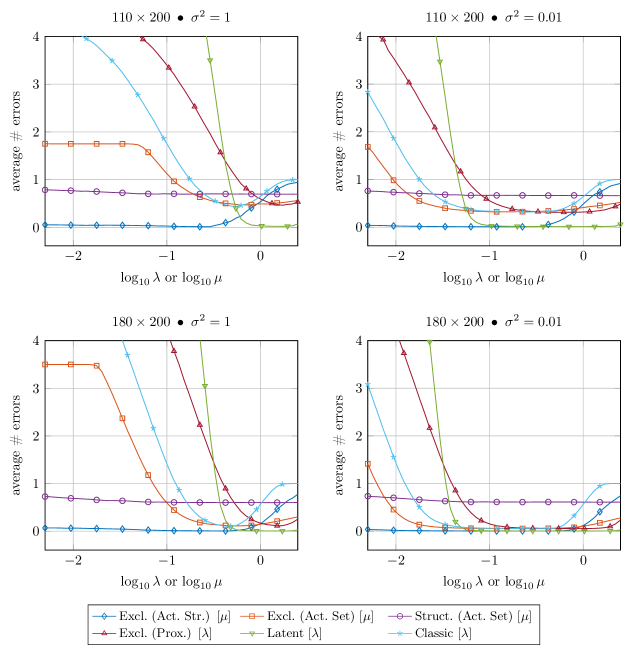
Figure 2: Average number of errors in the recovery of the signed support for different numbers of observations (top–bottom) and different noise variances (left–right).

Figure 2 shows the average number of errors in the recovery of the signed support for the six strategies above. We can observe that, when the regularizer parameter (either $\lambda$ or $\mu$) is properly set, both the algorithms presented in this paper—“Exclusive (Proximal)” and “Exclusive (Active Set)”—perform at least as well as the “Classic” Lasso regularizer. Note that no major gains were expected since the structure promoted by the exclusive group sparsity norm (that is, few uncorrelated active entries inside each group) is rather weak and not much more constraining than plain sparsity.

Nevertheless, the exclusive group sparsity is quite flexible and more rigid structures can be built upon it by including extra information. For instance, looking at the activation pattern of the parameter vector, we see that not only does it imply two active entries per group, but it also requires that entries from different groups are activated consecutively, forming a string. The “Active String” algorithm (a minor modification of the “Active Set”) has been designed to enforce this structure and, even though empirical, it provides the same performance as the “Latent” group Lasso, the natural choice for the activation pattern at hand.

As a final comment, the poor performance of the “Structured” Lasso algorithm was also expected since, as mentioned before, the promoted sparsity pattern (a single, continuous string) is not a match with the simulated activation pattern.

8 Conclusions

The paper provides a thorough characterization of the exclusive group sparsity norm and derives two efficient methods for solving optimization problems that include such norm as a regularizer. The effectiveness of the norm in promoting the desired sparsity is proven both theoretically, by studying asymptotic estimation consistency, and through simulations. Even though the exclusive group sparsity by itself does not offer a strong structure to exploit for support recovery, its flexibility allows tailoring the proposed optimization algorithms (specifically, the active set one) to fit more complex sparsity patterns and achieve performances that are as good as those of rigid, dedicated regularizers.

Acknowledgments

This work has been supported by the Spanish Government under grants TEC2014-59255-C3-1-R and RTI2018-099722-B-I00.

A General results

This appendix provides a set of theoretical tools which the proofs of Appendices B and C are built upon.

A.1 Notation and preliminary facts

Aiming at a self-contained paper, we review here some basic properties of the problems of the form

$$\operatorname*{minimize\,}_{\mathbf{x}\in\mathbb{R}^{p}}L(\mathbf{x})+\frac{\mu}{2}\Phi^{2}(\mathbf{x})$$

where $\Phi(\cdot)$ may be any norm in $\mathbb{R}^{p}$ and not necessarily the one defined in (1). By doing so, we will also introduce some notation that will prove useful in the following. It is worth mentioning that the results of this section are well known and a proof can be found in, e.g., Jenatton et al. (2011a).

Being interested in solutions with sparse support, we often deal with restricted versions of the loss function and of the norm. Namely, for a generic index set $\mathcal{I}\subseteq[p]$, the restricted loss function $L_{\mathcal{I}}(\mathbf{x}_{\mathcal{I}}):\mathbb{R}^{\lvert\mathcal{I}\rvert}\to\mathbb{R}_{+}$ maps $\mathbf{x}_{\mathcal{I}}$ to $L_{\mathcal{I}}(\mathbf{x}_{\mathcal{I}})=L({\mathbf{x}_{\{\mathcal{I}\}}})$, where we recall that ${\mathbf{x}_{\{\mathcal{I}\}}}\in\mathbb{R}^{p}$ is the “zero-padded” extension of $\mathbf{x}_{\mathcal{I}}$, that is $(\mathbf{x}_{\{\mathcal{I}\}})_{\mathcal{I}}=\mathbf{x}_{\mathcal{I}}$ and $(\mathbf{x}_{\{\mathcal{I}\}})_{\mathcal{I}^{\mathrm{c}}}=\mathbf{0}$. It is straightforward to see that $L_{\mathcal{I}}(\cdot)$ preserves the convexity and differentiability of $L(\cdot)$.

The restricted norm $\Phi_{\mathcal{I}}(\mathbf{x}_{\mathcal{I}})$, which is a proper norm, is defined accordingly. It is worth mentioning that, for the specific case of the exclusive group sparsity norm defined in (1), the restricted norm takes the form

$$\Omega_{\mathrm{excl},\mathcal{I}}(\mathbf{x}_{\mathcal{I}})=\sqrt{\sum_{G\in\mathcal{G}_{\mathcal{I}}}\lVert\mathbf{x}_{G\cap\mathcal{I}}\rVert_{1}^{2}}$$

where we recall that $\mathcal{G}_{\mathcal{I}}=\{G\in\mathcal{G}:G\cap\mathcal{I}\neq\emptyset\}$ is the subset of $\mathcal{G}$ with only groups that contain at least one index of $\mathcal{I}$.

Finally, for a dual characterization of the optimization problem, we also need to introduce two new functions $\mathbb{R}^{\lvert\mathcal{I}\rvert}\to\mathbb{R}_{+}$, namely

$$L_{\mathcal{I}}^{*}(\mathbf{u}_{\mathcal{I}}) =\sup_{\mathbf{x}_{\mathcal{I}}\in\mathbb{R}^{\lvert\mathcal{I}\rvert}}\mathbf{u}_{\mathcal{I}}^{\mathrm{T}}\mathbf{x}_{\mathcal{I}}-L_{\mathcal{I}}(\mathbf{x}_{\mathcal{I}})$$

$$\Phi_{\mathcal{I}}^{*}(\mathbf{u}_{\mathcal{I}}) =\sup_{\mathbf{x}_{\mathcal{I}}:\Phi_{\mathcal{I}}(\mathbf{x}_{\mathcal{I}})\leq 1}\mathbf{u}_{\mathcal{I}}^{\mathrm{T}}\mathbf{x}_{\mathcal{I}}$$

that is the Fenchel conjugate of $L_{\mathcal{I}}(\mathbf{x}_{\mathcal{I}})$ and the dual norm of $\Phi_{\mathcal{I}}(\mathbf{x}_{\mathcal{I}})$, respectively. Note that, even though $L_{\mathcal{I}}(\cdot)$ and $\Phi_{\mathcal{I}}(\cdot)$ extend to $L(\cdot)$ and $\Phi(\cdot)$ in the sense explained above, the same property does not hold, in general, for the Fenchel conjugates, $L_{\mathcal{I}}^{*}(\cdot)$ and $L^{*}(\cdot)$, or for the dual norms, $\Phi_{\mathcal{I}}^{*}(\cdot)$ and $\Phi^{*}(\cdot)$.

We are now in possession of all the tools needed to analyze the restricted minimization problem and its Fenchel dual, which read

$$\operatorname*{minimize\,}_{\mathbf{x}_{\mathcal{I}}\in\mathbb{R}^{\lvert\mathcal{I}\rvert}}L_{\mathcal{I}}(\mathbf{x}_{\mathcal{I}})+\frac{\mu}{2}\Phi_{\mathcal{I}}^{2}(\mathbf{x}_{\mathcal{I}})$$

$$\operatorname*{minimize\,}_{\mathbf{u}_{\mathcal{I}}\in\mathbb{R}^{\lvert\mathcal{I}\rvert}}L_{\mathcal{I}}^{*}(\mathbf{u}_{\mathcal{I}})+\frac{1}{2\mu}[\Phi_{\mathcal{I}}^{*}(\mathbf{u}_{\mathcal{I}})]^{2}$$

where we used the fact that the Fenchel conjugate of $\frac{\mu}{2}\Phi_{\mathcal{I}}^{2}(\cdot)$ is $\frac{1}{2\mu}[\Phi_{\mathcal{I}}^{*}(\cdot)]^{2}$ (Boyd and Vandenberghe, 2004, Example 3.27). From here, one can straightforwardly show (e.g., (Bertsekas, 2003, Proposition 5.3.8)) that strong duality holds and that the primal–dual optimal points $(\hat{\mathbf{x}_{\mathcal{I}}},\hat{\mathbf{u}_{\mathcal{I}}})$ are the only ones for which

$$\begin{cases}\hat{\mathbf{u}}_{\mathcal{I}}=\nabla L_{\mathcal{I}}(\hat{\mathbf{x}}_{\mathcal{I}})\\ \hat{\mathbf{u}}_{\mathcal{I}}\in-\partial\Bigl{[}\frac{\mu}{2}\Phi_{\mathcal{I}}^{2}\Bigr{]}(\hat{\mathbf{x}}_{\mathcal{I}})=-\mu\Phi_{\mathcal{I}}(\hat{\mathbf{x}}_{\mathcal{I}})\partial\Phi_{\mathcal{I}}(\hat{\mathbf{x}}_{\mathcal{I}}).\end{cases}$$ (27)

To understand the above point, we can simply realize that the duality gap of this problem is given by

$$\left(L_{\mathcal{I}}(\mathbf{x}_{\mathcal{I}})+L^{\ast}_{\mathcal{I}}(\mathbf{u}_{\mathcal{I}})-\mathbf{x}_{\mathcal{I}}^{\mathrm{T}}\mathbf{u}_{\mathcal{I}}\right)+\left(\frac{\mu}{2}\Phi_{\mathcal{I}}^{2}\left({\mathbf{x}}_{\mathcal{I}}\right)+\frac{1}{2\mu}\left[\Phi^{\ast}_{\mathcal{I}}\left({\mathbf{u}}_{\mathcal{I}}\right)\right]^{2}+\mathbf{x}_{\mathcal{I}}^{\mathrm{T}}\mathbf{u}_{\mathcal{I}}\right)$$ (28)

where the two terms inside parentheses are non-negative due to the Fenchel-Young inequality. Strong duality holds when we have equality in the two terms, which happens when the dual variable of each term ($\mathbf{u}_{\mathcal{I}}$ and $-\mathbf{u}_{\mathcal{I}}$ respectively) belongs to the subdifferential of the corresponding primal functions. In particular, the fist and second terms in parentheses respectively vanish if and only if the first and second conditions in (27) hold true.

Next, we reason that the second condition in (27) is equivalent to

$$-\hat{\mathbf{x}}_{\mathcal{I}}^{\mathrm{T}}\hat{\mathbf{u}}_{\mathcal{I}}=\mu\Phi_{\mathcal{I}}^{2}\left(\hat{\mathbf{x}}_{\mathcal{I}}\right)=\frac{1}{\mu}\left[\Phi^{\ast}_{\mathcal{I}}\left(\hat{\mathbf{u}}_{\mathcal{I}}\right)\right]^{2}.$$ (29)

On the one hand, as a direct consequence of the Fenchel-Young inequality, this condition holds if and only if

$$-\hat{\mathbf{x}}_{\mathcal{I}}^{\mathrm{T}}\hat{\mathbf{u}}_{\mathcal{I}}=\frac{\mu}{2}\Phi_{\mathcal{I}}^{2}\left(\hat{\mathbf{x}}_{\mathcal{I}}\right)+\frac{1}{2\mu}\left[\Phi^{\ast}_{\mathcal{I}}\left(\hat{\mathbf{u}}_{\mathcal{I}}\right)\right]^{2}$$ (30)

On the other hand, we recall from (7) that

$$\partial\Phi_{\mathcal{I}}(\hat{\mathbf{x}}_{\mathcal{I}})=\{\mathbf{z}_{\mathcal{I}}\in\mathbb{R}^{\lvert\mathcal{I}\rvert}:\mathbf{z}_{\mathcal{I}}^{\mathrm{T}}\hat{\mathbf{x}}_{\mathcal{I}}=\Phi_{\mathcal{I}}(\hat{\mathbf{x}}_{\mathcal{I}}),\quad\Phi_{\mathcal{I}}^{*}(\mathbf{z}_{\mathcal{I}})\leq 1\}.$$

Therefore, we have $\hat{\mathbf{u}}_{\mathcal{I}}\in-\mu\Phi_{\mathcal{I}}(\hat{\mathbf{x}}_{\mathcal{I}})\partial\Phi_{\mathcal{I}}(\hat{\mathbf{x}}_{\mathcal{I}})$ if and only if $\hat{\mathbf{u}}_{\mathcal{I}}$ is such that $\hat{\mathbf{u}}_{\mathcal{I}}^{\mathrm{T}}\hat{\mathbf{x}}_{\mathcal{I}}=-\mu\Phi^{2}_{\mathcal{I}}(\hat{\mathbf{x}}_{\mathcal{I}})$ and $\Phi_{\mathcal{I}}^{*}(\hat{\mathbf{u}}_{\mathcal{I}})\leq\mu\Phi_{\mathcal{I}}(\hat{\mathbf{x}}_{\mathcal{I}})$.

In summary, we see that the second condition in (27) implies that

$$\frac{\mu}{2}\Phi_{\mathcal{I}}^{2}(\hat{\mathbf{x}}_{\mathcal{I}})+\frac{1}{2\mu}[\Phi_{\mathcal{I}}^{*}(\hat{\mathbf{u}}_{\mathcal{I}})]^{2}=-\hat{\mathbf{x}}_{\mathcal{I}}^{\mathrm{T}}\hat{\mathbf{u}}_{\mathcal{I}}=\mu\Phi_{\mathcal{I}}^{2}(\hat{\mathbf{x}}_{\mathcal{I}}).$$

which directly leads to (29). Conversely, to see that the identity in (29) implies the second condition in (27) we only need to see that $\Phi_{\mathcal{I}}^{*}(\hat{\mathbf{u}}_{\mathcal{I}})\leq\mu\Phi_{\mathcal{I}}(\hat{\mathbf{x}}_{\mathcal{I}})$. But this follows directly from the definition of dual norm, which implies that $-\hat{\mathbf{x}}_{\mathcal{I}}^{\mathrm{T}}\hat{\mathbf{u}}_{\mathcal{I}}\leq\Phi_{\mathcal{I}}(\hat{\mathbf{x}}_{\mathcal{I}})\Phi_{\mathcal{I}}^{*}(\hat{\mathbf{u}}_{\mathcal{I}})$, so that using (30) we obtain

$$\frac{1}{\mu}\left[\Phi^{\ast}_{\mathcal{I}}\left(\hat{\mathbf{u}}_{\mathcal{I}}\right)\right]^{2}=-\hat{\mathbf{x}}_{\mathcal{I}}^{\mathrm{T}}\hat{\mathbf{u}}_{\mathcal{I}}\leq\Phi_{\mathcal{I}}(\hat{\mathbf{x}}_{\mathcal{I}})\Phi_{\mathcal{I}}^{*}(\hat{\mathbf{u}}_{\mathcal{I}})$$

as we wanted to show. Consequently, the primal–dual optimal points $(\hat{\mathbf{x}}_{\mathcal{I}},\hat{\mathbf{u}}_{\mathcal{I}})$ must satisfy

$$\begin{cases}\hat{\mathbf{u}}_{\mathcal{I}}=\nabla L_{\mathcal{I}}(\hat{\mathbf{x}}_{\mathcal{I}})\\ \hat{\mathbf{x}}_{\mathcal{I}}^{\mathrm{T}}\hat{\mathbf{u}}_{\mathcal{I}}=-\frac{1}{\mu}[\Phi_{\mathcal{I}}^{*}(\hat{\mathbf{u}}_{\mathcal{I}})]^{2}=-\mu\Phi_{\mathcal{I}}^{2}(\hat{\mathbf{x}}_{\mathcal{I}}).\end{cases}$$ (31)

In more general terms, assume that we have a pair of values $(\mathbf{x}_{\mathcal{I}},\mathbf{u}_{\mathcal{I}})$ that are not optimal points, but still chosen so that $\mathbf{u}_{\mathcal{I}}=\nabla L_{\mathcal{I}}(\mathbf{x}_{\mathcal{I}})$. According to the above reasoning, the first term in (28) is zero, so that the duality gap of the reduced problem takes the form

$$\frac{\mu}{2}\Phi_{\mathcal{I}}^{2}(\mathbf{x}_{\mathcal{I}})+\frac{1}{2\mu}[\Phi_{\mathcal{I}}^{*}(\mathbf{u}_{\mathcal{I}})]^{2}+\mathbf{x}_{\mathcal{I}}^{\mathrm{T}}\mathbf{u}_{\mathcal{I}}.$$

To conclude this section, we point out that these results hold for any index set $\mathcal{I}$ and, in particular, also for $\mathcal{I}=[p]$, which corresponds to the original (complete) problem. Then, we can characterize how well a primal–dual optimal point $(\hat{\mathbf{x}}_{\mathcal{I}},\hat{\mathbf{u}}_{\mathcal{I}})$ of the restricted problem behaves as a solution to the original problem. We recall here that $\hat{\mathbf{x}}_{\{\mathcal{I}\}}$ and $\hat{\mathbf{u}}_{\{\mathcal{I}\}}$ contain the primal/dual variable solutions of the restricted problem in the positions indexed by $\mathcal{I}$ and zeros elsewhere. Now, since $\mathbf{u}_{\mathcal{I}}=\nabla L_{\mathcal{I}}(\mathbf{x}_{\mathcal{I}})$ we must have $\mathbf{u}_{\{\mathcal{I}\}}=\nabla L(\mathbf{x}_{\{\mathcal{I}\}})$. Therefore, the solution to the restricted problem will achieve a duality gap:

$$\frac{\mu}{2}\Phi^{2}(\hat{\mathbf{x}}_{\{\mathcal{I}\}}) +\frac{1}{2\mu}[\Phi^{*}(\hat{\mathbf{u}}_{\{\mathcal{I}\}})]^{2}+\hat{\mathbf{x}}_{\{\mathcal{I}\}}^{\mathrm{T}}\hat{\mathbf{u}}_{\{\mathcal{I}\}}=\frac{\mu}{2}\Phi^{2}(\hat{\mathbf{x}}_{\{\mathcal{I}\}})+\frac{1}{2\mu}[\Phi^{*}(\hat{\mathbf{u}}_{\{\mathcal{I}\}})]^{2}+\hat{\mathbf{x}}_{\mathcal{I}}^{\mathrm{T}}\hat{\mathbf{u}}_{\mathcal{I}}$$

$$=\frac{\mu}{2}\Phi^{2}(\hat{\mathbf{x}}_{\{\mathcal{I}\}})+\frac{1}{2\mu}[\Phi^{*}(\hat{\mathbf{u}}_{\{\mathcal{I}\}})]^{2}-\frac{\mu}{2}\Phi_{\mathcal{I}}^{2}(\hat{\mathbf{x}}_{\mathcal{I}})-\frac{1}{2\mu}[\Phi_{\mathcal{I}}^{*}(\hat{\mathbf{u}}_{\mathcal{I}})]^{2}$$ (32)

$$=\frac{1}{2\mu}[\Phi^{*}(\hat{\mathbf{u}}_{\{\mathcal{I}\}})]^{2}-\frac{1}{2\mu}[\Phi_{\mathcal{I}}^{*}(\hat{\mathbf{u}}_{\mathcal{I}})]^{2}$$ (33)

where in (32) we have used the fact that the solution to the restricted problem achieves a zero duality gap and where in (33) we have used the definition of restricted norm.

A.2 Solution characterization

The following lemma further characterizes the solutions to (16) in terms of their support.

Lemma 9

Vector $\hat{\mathbf{x}}$, with support $\mathcal{J}=\operatorname{supp}\{\hat{\mathbf{x}}\}$, is a solution to

$$\operatorname*{minimize\,}_{\mathbf{x}\in\mathbb{R}^{p}}L(\mathbf{x})+\frac{\mu}{2}\Omega_{\mathrm{excl}}^{2}(\mathbf{x})$$

if and only if

$$\begin{cases}[\nabla L(\hat{\mathbf{x}})]_{\mathcal{J}}+\mu\hat{\mathbf{r}}_{\mathcal{J}}=\mathbf{0}\\ \max_{G\in\mathcal{G}_{\mathcal{J}}}\frac{\bigl{\lVert}[\nabla L(\hat{\mathbf{x}})]_{G\cap\mathcal{J}^{\mathrm{off}}}\bigr{\rVert}_{\infty}}{\lVert\hat{\mathbf{x}}_{G\cap\mathcal{J}}\rVert_{1}}\leq\mu\\ [\nabla L(\hat{\mathbf{x}})]_{\mathcal{J}^{\mathrm{inact.}}}=\mathbf{0}\end{cases}$$ (34)

where $\hat{\mathbf{r}}\in\mathbb{R}^{p}$ is a vector with entries

$$\hat{r}_{i}=\begin{cases}\lVert\hat{\mathbf{x}}_{G_{i}\cap\mathcal{J}}\rVert_{1}\operatorname{sign}(\hat{x}_{i})&\text{if }i\in\mathcal{J}\\ 0&\text{if }i\in\mathcal{J}^{\mathrm{c}}\end{cases}$$ (35)

with $G_{i}$ the (unique) group containing index $i$, and where $\mathcal{J}^{\mathrm{off}}=\{i\in\mathcal{J}^{\mathrm{c}}\cap G,\forall G\in\mathcal{G}_{\mathcal{J}}\}$ is the set of inactive entries belonging to active groups. Finally, we denote by $\mathcal{J}^{\mathrm{inact.}}=\mathcal{J}^{\mathrm{c}}\setminus\mathcal{J}^{\mathrm{off}}$ the set of indices belonging to inactive groups.

Moreover, solution $\hat{\mathbf{x}}$ also satisfies the following inequalities:

$$\begin{cases}\Omega_{\mathrm{excl},\mathcal{J}}^{*}\bigl{(}[\nabla L(\hat{\mathbf{x}})]_{\mathcal{J}}\bigr{)}\leq\mu\Omega_{\mathrm{excl}}(\hat{\mathbf{x}})\\ \Omega_{\mathrm{excl},{\mathcal{J}^{\mathrm{off}}}}^{*}\bigl{(}[\nabla L(\hat{\mathbf{x}})]_{\mathcal{J}^{\mathrm{off}}}\bigr{)}\leq\mu\Omega_{\mathrm{excl}}(\hat{\mathbf{x}})\\ \Omega_{\mathrm{excl}}^{*}(\nabla L(\hat{\mathbf{x}}))\leq\mu\Omega_{\mathrm{excl}}(\hat{\mathbf{x}}).\end{cases}$$

Proof  For the purpose of this proof, let $F(\mathbf{x})=L(\mathbf{x})+\frac{\mu}{2}\Omega_{\mathrm{excl}}^{2}(\mathbf{x})$. Then, by convexity, vector $\hat{\mathbf{x}}$ is a solution to (16) if and only if

$$\lim_{\epsilon\to 0^{+}}\frac{F(\hat{\mathbf{x}}+\epsilon\mathbf{w})-F(\hat{\mathbf{x}})}{\epsilon}\geq 0$$

for all directions $\mathbf{w}\in\mathbb{R}^{p}$. In order to see the implications of the above inequality, we first need to show that it can be equivalently rewritten as

$$\mathbf{w}^{\mathrm{T}}\nabla L(\hat{\mathbf{x}})+\mu\hat{\mathbf{r}}_{\mathcal{J}}^{\mathrm{T}}\mathbf{w}_{\mathcal{J}}+\mu\sum_{G\in\mathcal{G}_{\mathcal{J}}}\lVert\hat{\mathbf{x}}_{G\cap\mathcal{J}}\rVert_{1}\lVert\mathbf{w}_{G\cap\mathcal{J}^{\mathrm{c}}}\rVert_{1}\geq 0.$$ (36)

Indeed, recalling the definition of $\Omega_{\mathrm{excl}}(\cdot)$, one has

$$\Omega_{\mathrm{excl}}^{2}(\hat{\mathbf{x}}+\epsilon\mathbf{w}) =\sum_{G\in\mathcal{G}}\Biggl{(}\sum_{i\in G}\lvert\hat{x}_{i}+\epsilon w_{i}\rvert\Biggr{)}^{2}$$

$$=\sum_{G\in\mathcal{G}_{\mathcal{J}}}\Biggl{(}\sum_{i\in G\cap\mathcal{J}}\lvert\hat{x}_{i}+\epsilon w_{i}\rvert+\epsilon\sum_{i\in G\cap\mathcal{J}^{\mathrm{c}}}\lvert w_{i}\rvert\Biggr{)}^{2}+\epsilon^{2}\sum_{G\in\mathcal{G}_{\mathcal{J}}^{\mathrm{c}}}\Biggl{(}\sum_{i\in G}\lvert w_{i}\rvert\Biggr{)}^{2}.$$

Now, let us define $\mathbf{s}=\operatorname{sign}(\hat{\mathbf{x}})$ element-wise. Moreover, since $\epsilon$ is arbitrarily small, we can assume that $\hat{x}_{i}+\epsilon w_{i}$ keeps the same sign as $\hat{x}_{i}$. It follows that

$$\Omega_{\mathrm{excl}}^{2}(\hat{\mathbf{x}}+\epsilon\mathbf{w}) =\sum_{G\in\mathcal{G}_{\mathcal{J}}}\Bigl{(}\lVert\hat{\mathbf{x}}_{G\cap\mathcal{J}}\rVert_{1}+\epsilon\mathbf{s}_{G\cap\mathcal{J}}^{\mathrm{T}}\mathbf{w}_{G\cap\mathcal{J}}+\epsilon\lVert\mathbf{w}_{G\cap\mathcal{J}^{\mathrm{c}}}\rVert_{1}\Bigr{)}^{2}+\epsilon^{2}\sum_{G\in\mathcal{G}_{\mathcal{J}}^{\mathrm{c}}}\lVert\mathbf{w}_{G}\rVert_{1}^{2}$$

$$=\Omega_{\mathrm{excl},\mathcal{J}}^{2}(\hat{\mathbf{x}}_{\mathcal{J}})+2\epsilon\sum_{G\in\mathcal{G}_{\mathcal{J}}}\lVert\hat{\mathbf{x}}_{G\cap\mathcal{J}}\rVert_{1}\Bigl{(}\mathbf{s}_{G\cap\mathcal{J}}^{\mathrm{T}}\mathbf{w}_{G\cap\mathcal{J}}+\lVert\mathbf{w}_{G\cap\mathcal{J}^{\mathrm{c}}}\rVert_{1}\Bigr{)}+o(\epsilon)$$

$$=\Omega_{\mathrm{excl},\mathcal{J}}^{2}(\hat{\mathbf{x}}_{\mathcal{J}})+2\epsilon\hat{\mathbf{r}}_{\mathcal{J}}^{\mathrm{T}}\mathbf{w}_{\mathcal{J}}+2\epsilon\sum_{G\in\mathcal{G}_{\mathcal{J}}}\lVert\hat{\mathbf{x}}_{G\cap\mathcal{J}}\rVert_{1}\lVert\mathbf{w}_{G\cap\mathcal{J}^{\mathrm{c}}}\rVert_{1}+o(\epsilon)$$

where we have used the definition of $\hat{\mathbf{r}}$ given in (35). By plugging the last line into the definition of $F(\hat{\mathbf{x}}+\epsilon\mathbf{w})$, one readily obtains (36).

Now, (34) is a straightforward consequence of the fact that (36) must hold for all $\mathbf{w}$ and, specifically,

$$\inf_{\mathbf{w}:\operatorname{supp}\{\mathbf{w}\}\subseteq\mathcal{I}}\Bigl{\{}\mathbf{w}^{\mathrm{T}}\nabla L(\hat{\mathbf{x}})+\mu\hat{\mathbf{r}}_{\mathcal{J}}^{\mathrm{T}}\mathbf{w}_{\mathcal{J}}+\mu\sum_{G\in\mathcal{G}_{\mathcal{J}}}\lVert\hat{\mathbf{x}}_{G\cap\mathcal{J}}\rVert_{1}\lVert\mathbf{w}_{G\cap\mathcal{J}^{\mathrm{c}}}\rVert_{1}\Bigr{\}}\geq 0$$

for $\mathcal{I}\in\{\mathcal{J},\mathcal{J}^{\mathrm{off}},\mathcal{J}^{\mathrm{inact.}}\}$.

To prove the second part of the lemma, let us start by noting that

$$\mathbf{w}_{\mathcal{J}}^{\mathrm{T}}\hat{\mathbf{r}}_{\mathcal{J}} =\sum_{G\in\mathcal{G}_{\mathcal{J}}}\lVert\hat{\mathbf{x}}_{G\cap\mathcal{J}}\rVert_{1}\sum_{i\in G\cap\mathcal{J}}w_{i}\operatorname{sign}(\hat{x}_{i})$$

$$\leq\sum_{G\in\mathcal{G}_{\mathcal{J}}}\lVert\hat{\mathbf{x}}_{G\cap\mathcal{J}}\rVert_{1}\sum_{i\in G\cap\mathcal{J}}\lvert w_{i}\rvert$$

$$=\sum_{G\in\mathcal{G}_{\mathcal{J}}}\lVert\hat{\mathbf{x}}_{G\cap\mathcal{J}}\rVert_{1}\lVert\mathbf{w}_{G\cap\mathcal{J}}\rVert_{1}$$ (37)

$$\overset{(\mathrm{a})}{\leq}\sqrt{\sum_{G\in\mathcal{G}_{\mathcal{J}}}\lVert\hat{\mathbf{x}}_{G\cap\mathcal{J}}\rVert_{1}^{2}}\sqrt{\sum_{G\in\mathcal{G}_{\mathcal{J}}}\lVert\mathbf{w}_{G\cap\mathcal{J}}\rVert_{1}^{2}}$$

$$=\Omega_{\mathrm{excl},\mathcal{J}}(\hat{\mathbf{x}}_{\mathcal{J}})\Omega_{\mathrm{excl},\mathcal{J}}(\mathbf{w}_{\mathcal{J}})$$

where $(\mathrm{a})$ is an application of the Cauchy–Schwartz inequality, which also applies to the last term of (36) yielding

$$\sum_{G\in\mathcal{G}_{\mathcal{J}}}\lVert\hat{\mathbf{x}}_{G\cap\mathcal{J}}\rVert_{1}\lVert\mathbf{w}_{G\cap\mathcal{J}^{\mathrm{c}}}\rVert_{1}\leq\Omega_{\mathrm{excl},\mathcal{J}}(\hat{\mathbf{x}}_{\mathcal{J}})\Omega_{\mathrm{excl},{\mathcal{J}^{\mathrm{off}}}}(\mathbf{w}_{\mathcal{J}^{\mathrm{off}}}).$$

As a result, the left-hand side of (36) can be upper-bounded by

$$\mathbf{w}^{\mathrm{T}}\nabla L(\hat{\mathbf{x}}) +\mu\Omega_{\mathrm{excl},\mathcal{J}}(\hat{\mathbf{x}}_{\mathcal{J}})\Bigl{(}\Omega_{\mathrm{excl},\mathcal{J}}(\mathbf{w}_{\mathcal{J}})+\Omega_{\mathrm{excl},{\mathcal{J}^{\mathrm{off}}}}(\mathbf{w}_{\mathcal{J}^{\mathrm{off}}})\Bigr{)}$$

$$\geq\mathbf{w}^{\mathrm{T}}\nabla L(\hat{\mathbf{x}})+\mu\hat{\mathbf{r}}_{\mathcal{J}}^{\mathrm{T}}\mathbf{w}_{\mathcal{J}}+\mu\sum_{G\in\mathcal{G}_{\mathcal{J}}}\lVert\hat{\mathbf{x}}_{G\cap\mathcal{J}}\rVert_{1}\lVert\mathbf{w}_{G\cap\mathcal{J}^{\mathrm{c}}}\rVert_{1}\geq 0.$$

Since, once again, the above inequality must hold for all $\mathbf{w}\in\mathbb{R}^{p}$ and, by taking the infimum over all $\mathbf{w}$ with support in $\mathcal{J}$ and $\mathcal{J}^{\mathrm{off}}$, we obtain

$$\begin{cases}\Omega_{\mathrm{excl},\mathcal{J}}^{*}\bigl{(}[\nabla L(\hat{\mathbf{x}})]_{\mathcal{J}}\bigr{)}\leq\mu\Omega_{\mathrm{excl}}(\hat{\mathbf{x}})\\ \Omega_{\mathrm{excl},{\mathcal{J}^{\mathrm{off}}}}^{*}\bigl{(}[\nabla L(\hat{\mathbf{x}})]_{\mathcal{J}^{\mathrm{off}}}\bigr{)}\leq\mu\Omega_{\mathrm{excl}}(\hat{\mathbf{x}})\end{cases}$$

respectively. The same trick can be applied to show

$$\Omega_{\mathrm{excl}}^{*}(\nabla L(\hat{\mathbf{x}}))\leq\mu\Omega_{\mathrm{excl}}(\hat{\mathbf{x}}).$$

Indeed, one has

$$\Omega_{\mathrm{excl}}(\mathbf{w}) =\sqrt{\sum_{G\in\mathcal{G}}\lVert\mathbf{w}_{G}\rVert_{1}^{2}}$$

$$\geq\sqrt{\sum_{G\in\mathcal{G}_{\mathcal{J}}}\lVert\mathbf{w}_{G}\rVert_{1}^{2}}$$

$$=\frac{1}{\Omega_{\mathrm{excl},\mathcal{J}}(\hat{\mathbf{x}}_{\mathcal{J}})}\sqrt{\sum_{G\in\mathcal{G}_{\mathcal{J}}}\lVert\hat{\mathbf{x}}_{G\cap\mathcal{J}}\rVert_{1}^{2}}\sqrt{\sum_{G\in\mathcal{G}_{\mathcal{J}}}\lVert\mathbf{w}_{G}\rVert_{1}^{2}}$$

$$\geq\frac{1}{\Omega_{\mathrm{excl},\mathcal{J}}(\hat{\mathbf{x}}_{\mathcal{J}})}\sum_{G\in\mathcal{G}_{\mathcal{J}}}\lVert\hat{\mathbf{x}}_{G\cap\mathcal{J}}\rVert_{1}\lVert\mathbf{w}_{G}\rVert_{1}$$

$$=\frac{1}{\Omega_{\mathrm{excl},\mathcal{J}}(\hat{\mathbf{x}}_{\mathcal{J}})}\sum_{G\in\mathcal{G}_{\mathcal{J}}}\lVert\hat{\mathbf{x}}_{G\cap\mathcal{J}}\rVert_{1}\Bigl{(}\lVert\mathbf{w}_{G\cap\mathcal{J}}\rVert_{1}+\lVert\mathbf{w}_{G\cap\mathcal{J}^{\mathrm{c}}}\rVert_{1}\Bigr{)}$$

$$\geq\frac{\hat{\mathbf{r}}_{\mathcal{J}}^{\mathrm{T}}\mathbf{w}_{\mathcal{J}}}{\Omega_{\mathrm{excl},\mathcal{J}}(\hat{\mathbf{x}}_{\mathcal{J}})}+\frac{1}{\Omega_{\mathrm{excl},\mathcal{J}}(\hat{\mathbf{x}}_{\mathcal{J}})}\sum_{G\in\mathcal{G}_{\mathcal{J}}}\lVert\hat{\mathbf{x}}_{G\cap\mathcal{J}}\rVert_{1}\lVert\mathbf{w}_{G\cap\mathcal{J}^{\mathrm{c}}}\rVert_{1}$$

which implies

$$\mathbf{w}^{\mathrm{T}}\nabla L(\hat{\mathbf{x}})+\mu\Omega_{\mathrm{excl},\mathcal{J}}(\hat{\mathbf{x}}_{\mathcal{J}})\Omega_{\mathrm{excl}}(\mathbf{w})\geq\mathbf{w}^{\mathrm{T}}\nabla L(\hat{\mathbf{x}})+\mu\hat{\mathbf{r}}_{\mathcal{J}}^{\mathrm{T}}\mathbf{w}_{\mathcal{J}}+\mu\sum_{G\in\mathcal{G}_{\mathcal{J}}}\lVert\hat{\mathbf{x}}_{G\cap\mathcal{J}}\rVert_{1}\lVert\mathbf{w}_{G\cap\mathcal{J}^{\mathrm{c}}}\rVert_{1}\geq 0.$$

Finally, we only need to take the infimum over all possible $\mathbf{w}$ and recall that $\Omega_{\mathrm{excl},\mathcal{J}}(\hat{\mathbf{x}}_{\mathcal{J}})=\Omega_{\mathrm{excl}}(\hat{\mathbf{x}})$ since $\operatorname{supp}\{\hat{\mathbf{x}}\}=\mathcal{J}$.  

For the proof of Proposition 7, we will also make use of the following simple result.

Lemma 10

For any vector $\mathbf{u}\in\mathbb{R}^{p}$ and any index subset $\mathcal{J}\in[p]$, the dual norm $\Omega_{\mathrm{excl}}^{*}(\mathbf{u})$ can be upper-bounded by

$$\Omega_{\mathrm{excl}}^{*}(\mathbf{u})\leq\max\{\Omega_{\mathrm{excl},\mathcal{J}}^{*}(\mathbf{u}_{\mathcal{J}}),\Omega_{\mathrm{excl},{\mathcal{J}^{\mathrm{off}}}}^{*}(\mathbf{u}_{\mathcal{J}^{\mathrm{off}}}),\Omega_{\mathrm{excl},{\mathcal{J}^{\mathrm{inact.}}}}^{*}(\mathbf{u}_{\mathcal{J}^{\mathrm{inact.}}})\}.$$

Proof  By definition of dual norm, we have

$$\Omega_{\mathrm{excl}}^{*}(\mathbf{u}) =\max_{\mathbf{v}\in\mathbb{R}^{p}}\mathbf{u}^{\mathrm{T}}\mathbf{v}\quad\text{s.to }\Omega_{\mathrm{excl}}(\mathbf{v})\leq 1$$

$$=\max_{\mathbf{v}\in\mathbb{R}^{p}}\mathbf{u}^{\mathrm{T}}\mathbf{v}\quad\text{s.to }\sum_{G\in\mathcal{G}}\lVert\mathbf{v}_{G}\rVert_{1}^{2}\leq 1$$

$$=\max_{\mathbf{v}\in\mathbb{R}^{p}}\mathbf{u}^{\mathrm{T}}\mathbf{v}\quad\text{s.to }\sum_{G\in\mathcal{G}_{\mathcal{J}}}\lVert\mathbf{v}_{G}\rVert_{1}^{2}+\sum_{G\in\mathcal{G}_{\mathcal{J}^{\mathrm{inact.}}}}\lVert\mathbf{v}_{G}\rVert_{1}^{2}\leq 1$$

$$=\max_{\mathbf{v}\in\mathbb{R}^{p}}\mathbf{u}^{\mathrm{T}}\mathbf{v}\quad\text{s.to }\sum_{G\in\mathcal{G}_{\mathcal{J}}}\Bigl{(}\lVert\mathbf{v}_{G\cap\mathcal{J}}\rVert_{1}+\lVert\mathbf{v}_{G\cap\mathcal{J}^{\mathrm{off}}}\rVert_{1}\Bigr{)}^{2}+\sum_{G\in\mathcal{G}_{\mathcal{J}^{\mathrm{inact.}}}}\lVert\mathbf{v}_{G}\rVert_{1}^{2}\leq 1$$

$$\leq\max_{\mathbf{v}\in\mathbb{R}^{p}}\mathbf{u}^{\mathrm{T}}\mathbf{v}\quad\text{s.to }\sum_{G\in\mathcal{G}_{\mathcal{J}}}\lVert\mathbf{v}_{G\cap\mathcal{J}}\rVert_{1}^{2}+\sum_{G\in\mathcal{G}_{\mathcal{J}}}\lVert\mathbf{v}_{G\cap\mathcal{J}^{\mathrm{off}}}\rVert_{1}^{2}+\sum_{G\in\mathcal{G}_{\mathcal{J}^{\mathrm{inact.}}}}\lVert\mathbf{v}_{G}\rVert_{1}^{2}\leq 1$$

$$=\max_{\mathbf{v}\in\mathbb{R}^{p},a,b,c}\mathbf{u}^{\mathrm{T}}\mathbf{v}$$

$$\phantom{=mt}\text{s.to }\sum_{G\in\mathcal{G}_{\mathcal{J}}}\lVert\mathbf{v}_{G\cap\mathcal{J}}\rVert_{1}^{2}\leq a,\quad\sum_{G\in\mathcal{G}_{\mathcal{J}}}\lVert\mathbf{v}_{G\cap\mathcal{J}^{\mathrm{off}}}\rVert_{1}^{2}\leq b,\quad\sum_{G\in\mathcal{G}_{\mathcal{J}^{\mathrm{inact.}}}}\lVert\mathbf{v}_{G}\rVert_{1}^{2}\leq c,$$

$$\phantom{=mt\text{s.to }}a+b+c\leq 1.$$

Since sets $\mathcal{J}$, $\mathcal{J}^{\mathrm{off}}$ and $\mathcal{J}^{\mathrm{inact.}}$ form a partition of $[p]$, the result is straightforward (see also (Jenatton et al., 2011a, Lemma 15)).  

B Active set: Proofs

This section provides a proof of Propositions 6 and 7, the two building blocks of the active set algorithm described in Section 5.

B.1 Proof of Proposition 6

Suppose vector $\hat{\mathbf{x}}$ is a solution to (16). Then, (18) has already been proven as a part of Lemma 9 and we only need to focus on (17). The approach follows the same lines as the proof of Lemma 9: Starting from (36), which is necessary and sufficient for vector $\hat{\mathbf{x}}$ with support $\mathcal{J}$ to be a solution to (16), we project the right-hand side onto an accurately chosen subspace to derive the desired necessary condition.

More specifically, we focus on vectors with support in $\mathcal{K}\in\Pi(\mathcal{J})$ and project onto the set of indices $\mathcal{K}\setminus\mathcal{J}$, for any $\mathcal{K}\in\Pi(\mathcal{J})$. Then, (36) takes the form

$$\mathbf{w}_{\mathcal{K}\setminus\mathcal{J}}^{\mathrm{T}}[\nabla L(\hat{\mathbf{x}})]_{\mathcal{K}\setminus\mathcal{J}}+\mu\sum_{G\in\mathcal{G}_{\mathcal{J}}\cap\mathcal{G}_{\mathcal{K}\setminus\mathcal{J}}}\lVert\hat{\mathbf{x}}_{G\cap\mathcal{J}}\rVert_{1}\lVert\mathbf{w}_{G\cap(\mathcal{K}\setminus\mathcal{J})}\rVert_{1}\geq 0.$$

Since, as already proven, $[\nabla L(\hat{\mathbf{x}})]_{i}=0$ for all $i\in\mathcal{J}^{\mathrm{inact.}}$, we can further simplify the last inequality and write

$$\sum_{G\in\mathcal{G}_{\mathcal{J}}\cap\mathcal{G}_{\mathcal{K}\setminus\mathcal{J}}}\mathbf{w}_{G\cap(\mathcal{K}\setminus\mathcal{J})}^{\mathrm{T}}[\nabla L(\hat{\mathbf{x}})]_{G\cap(\mathcal{K}\setminus\mathcal{J})}+\mu\sum_{G\in\mathcal{G}_{\mathcal{J}}\cap\mathcal{G}_{\mathcal{K}\setminus\mathcal{J}}}\lVert\hat{\mathbf{x}}_{G\cap\mathcal{J}}\rVert_{1}\lVert\mathbf{w}_{G\cap(\mathcal{K}\setminus\mathcal{J})}\rVert_{1}\geq 0.$$

By recalling that the inequality must hold for all $\mathbf{w}$ and exploiting the fact that the index sets $G\in\mathcal{G}$ are disjoint, we obtain the equivalent form

$$\sum_{G\in\mathcal{G}_{\mathcal{J}}\cap\mathcal{G}_{\mathcal{K}\setminus\mathcal{J}}}\inf_{\mathbf{w}_{G\cap(\mathcal{K}\setminus\mathcal{J})}}\Bigl{\{}\mathbf{w}_{G\cap(\mathcal{K}\setminus\mathcal{J})}^{\mathrm{T}}[\nabla L(\hat{\mathbf{x}})]_{G\cap(\mathcal{K}\setminus\mathcal{J})}+\mu\lVert\hat{\mathbf{x}}_{G\cap\mathcal{J}}\rVert_{1}\lVert\mathbf{w}_{G\cap(\mathcal{K}\setminus\mathcal{J})}\rVert_{1}\Bigr{\}}\geq 0$$

which implies

$$\max_{G\in\mathcal{G}_{\mathcal{J}}\cap\mathcal{G}_{\mathcal{K}\setminus\mathcal{J}}}\frac{\Bigl{\lVert}[\nabla L(\hat{\mathbf{x}})]_{G\cap(\mathcal{K}\setminus\mathcal{J})}\Bigr{\rVert}_{\infty}}{\lVert\hat{\mathbf{x}}_{G\cap\mathcal{J}}\rVert_{1}}\leq\mu.$$

Being $\mathcal{K}\in\Pi(\mathcal{J})$ arbitrarily chosen, Proposition 6 is proven.

B.2 Proof of Proposition 7

Let $\hat{\mathbf{u}}=\nabla L(\hat{\mathbf{x}})$ and $\hat{\mathbf{u}}_{\mathcal{J}}=\nabla L_{\mathcal{J}}(\hat{\mathbf{x}}_{\mathcal{J}})$ be the feasible dual points associated to $\hat{\mathbf{x}}$ (and, in turn, to $\hat{\mathbf{x}}_{\mathcal{J}}$) as a solution to the full and restricted problems, respectively. Note that the notation is consistent since, indeed, $[\nabla L(\hat{\mathbf{x}})]_{j}=[\nabla L_{\mathcal{J}}(\hat{\mathbf{x}}_{\mathcal{J}})]_{j}$ for all $j\in\mathcal{J}$. However, in general, $[\nabla L(\hat{\mathbf{x}})]_{j}\neq 0$ for $j\notin\mathcal{J}$ and, equivalently, $\hat{\mathbf{u}}\neq\hat{\mathbf{u}}_{\{\mathcal{J}\}}$, that is $\hat{\mathbf{u}}$ may be non-zero outside the support of $\hat{\mathbf{x}}$.

As proven in Section A.1, the duality gap obtained by considering $\hat{\mathbf{x}}$ as a solution to the full problem is given by (33). Then, by Lemma 10, this duality gap can be majorized by

$$\frac{1}{2\mu}[\Omega_{\mathrm{excl}}^{*}(\hat{\mathbf{u}})]^{2}-\frac{1}{2\mu}[\Omega_{\mathrm{excl},\mathcal{J}}^{*}(\hat{\mathbf{u}}_{\mathcal{J}})]^{2}\\ \leq\frac{1}{2\mu}\max\Bigl{\{}0,[\Omega_{\mathrm{excl},\mathcal{J}}^{*}(\hat{\mathbf{u}}_{\mathcal{J}^{\mathrm{off}}})]^{2}-[\Omega_{\mathrm{excl},\mathcal{J}}^{*}(\hat{\mathbf{u}}_{\mathcal{J}})]^{2},[\Omega_{\mathrm{excl},{\mathcal{J}^{\mathrm{inact.}}}}^{*}(\hat{\mathbf{u}}_{\mathcal{J}^{\mathrm{inact.}}})]^{2}-[\Omega_{\mathrm{excl},\mathcal{J}}^{*}(\hat{\mathbf{u}}_{\mathcal{J}})]^{2}\Bigr{\}}$$

Then, to achieve a duality gap smaller than $\epsilon$, it suffices that

$$\begin{cases}[\Omega_{\mathrm{excl},{\mathcal{J}^{\mathrm{off}}}}^{*}(\hat{\mathbf{u}}_{\mathcal{J}^{\mathrm{off}}})]^{2}\leq 2\mu\epsilon+[\Omega_{\mathrm{excl},\mathcal{J}}^{*}(\hat{\mathbf{u}}_{\mathcal{J}})]^{2}\\ [\Omega_{\mathrm{excl},{\mathcal{J}^{\mathrm{inact.}}}}^{*}(\hat{\mathbf{u}}_{\mathcal{J}^{\mathrm{inact.}}})]^{2}\leq 2\mu\epsilon+[\Omega_{\mathrm{excl},\mathcal{J}}^{*}(\hat{\mathbf{u}}_{\mathcal{J}})]^{2}.\end{cases}$$

The lemma comes from the definition of the (restricted) dual norm, the fact that we set $\hat{\mathbf{u}}=\nabla L(\hat{\mathbf{x}})$ and (31).

C Proof of Theorem 8

The proof capitalizes on the results of Wainwright (2009) and references therein. We summarize next the salient points and refer to those papers for more specific technical results.

We first point out that a certain $\check{\mathbf{x}}_{n}\in\mathbb{R}^{p}$ is an optimal solution of the problem in (20) if and only if there exists a subgradient $\check{\mathbf{u}}_{n}\in\partial\Omega_{\mathrm{excl}}(\mathbf{x})$ at $\mathbf{x}=\check{\mathbf{x}}_{n}$ such that

$$\frac{1}{n}\mathbf{A}_{n}^{\mathrm{T}}\mathbf{A}_{n}\left(\check{\mathbf{x}}_{n}-\mathbf{x}_{n}^{\ast}\right)-\frac{1}{n}\mathbf{A}_{n}^{\mathrm{T}}\mathbf{w}_{n}+\lambda_{n}\check{\mathbf{u}}_{n}=\mathbf{0}$$ (38)

where we have used the fact that $\mathbf{y}_{n}=\mathbf{A}_{n}\mathbf{x}_{n}^{\ast}+\mathbf{w}_{n}$. Following the steps in Wainwright (2009), we will now construct a sequence of pairs $(\check{\mathbf{x}}_{n},\check{\mathbf{u}}_{n})\in\mathbb{R}^{p}\times\mathbb{R}^{p}$ and check under which asymptotic conditions they are solutions to (38). It is worth remarking that, even though at a first glance it may seem that the true support $\mathcal{J}=\operatorname{supp}(\mathbf{x}_{n}^{*})$ is assumed to be known, the argument below provides a set of equivalent conditions that, if met, ensure that $\mathcal{J}$ is the correct support and, more importantly, that $\operatorname{\mathbb{S}_{\pm}}(\check{\mathbf{x}})=\operatorname{\mathbb{S}_{\pm}}(\mathbf{x}^{*})$. Therefore, any efficient method for solving (20) will converge towards the correct solution when $\lambda_{n}$ is properly set.

On the one hand, we consider first a vector $\check{\mathbf{x}}_{n}\in\mathbb{R}^{p}$ that is built as follows. Take $\check{\mathbf{x}}_{\mathcal{J}}\in\mathbb{R}^{|\mathcal{J}|}$ as the unique solution to the following restricted problem:

$$\check{\mathbf{x}}_{\mathcal{J}}=\arg\min_{\mathbf{x}_{\mathcal{J}}\in\mathbb{R}^{|\mathcal{J}|}}\left\{\frac{1}{2n}\lVert\mathbf{y}_{n}-\mathbf{A}_{\mathcal{J}}\mathbf{x}_{\mathcal{J}}\rVert_{2}^{2}+\lambda_{n}\Omega_{\mathrm{excl},\mathcal{J}}(\mathbf{x}_{\mathcal{J}})\right\}$$ (39)

and force $\check{\mathbf{x}}_{\mathcal{J}^{\mathrm{c}}}=0$. On the other hand, we choose $\check{\mathbf{u}}_{n}\in\mathbb{R}^{p}$ by first taking $\check{\mathbf{u}}_{\mathcal{J}}$ to be any subgradient of $\Omega_{\mathrm{excl},\mathcal{J}}(\mathbf{x}_{\mathcal{J}})$ at the point $\check{\mathbf{x}}_{\mathcal{J}}$. Then, $\check{\mathbf{u}}_{\mathcal{J}^{\mathrm{c}}}$ is fixed so that the complete vector $\check{\mathbf{u}}_{n}$ is a solution to the optimality condition of the global problem in (38). This is possible because we can express this condition as

$$\frac{1}{n}\begin{bmatrix}\mathbf{A}_{\mathcal{J}}^{\mathrm{T}}\mathbf{A}_{\mathcal{J}}&\mathbf{A}_{\mathcal{J}}^{\mathrm{T}}\mathbf{A}_{\mathcal{J}^{\mathrm{c}}}\\ \mathbf{A}_{\mathcal{J}^{\mathrm{c}}}^{\mathrm{T}}\mathbf{A}_{\mathcal{J}}&\mathbf{A}_{\mathcal{J}^{\mathrm{c}}}^{\mathrm{T}}\mathbf{A}_{\mathcal{J}^{\mathrm{c}}}\end{bmatrix}\begin{bmatrix}\check{\mathbf{x}}_{\mathcal{J}}-\mathbf{x}_{\mathcal{J}}^{\ast}\\ \mathbf{0}\end{bmatrix}-\frac{1}{n}\begin{bmatrix}\mathbf{A}_{\mathcal{J}}^{\mathrm{T}}\\ \mathbf{A}^{\mathrm{T}}_{\mathcal{J}^{\mathrm{c}}}\end{bmatrix}\mathbf{w}_{n}+\lambda_{n}\begin{bmatrix}\check{\mathbf{u}}_{\mathcal{J}}\\ \check{\mathbf{u}}_{\mathcal{J}^{\mathrm{c}}}\end{bmatrix}=\mathbf{0}$$

so that we only need to choose

$$\check{\mathbf{u}}_{\mathcal{J}^{\mathrm{c}}}=\mathbf{A}_{\mathcal{J}^{\mathrm{c}}}^{\mathrm{T}}\left[\mathbf{A}_{\mathcal{J}}\left(\mathbf{A}_{\mathcal{J}}^{\mathrm{T}}\mathbf{A}_{\mathcal{J}}\right)^{-1}\check{\mathbf{u}}_{\mathcal{J}}+\frac{1}{n\lambda_{n}}\Pi_{\mathbf{A}_{\mathcal{J}}^{\perp}}\mathbf{w}_{n}\right]$$ (40)

where $\Pi_{\mathbf{A}_{\mathcal{J}}^{\perp}}=\mathbf{I}_{p}-\mathbf{A}_{\mathcal{J}}\left(\mathbf{A}_{\mathcal{J}}^{\mathrm{T}}\mathbf{A}_{\mathcal{J}}\right)^{-1}\mathbf{A}_{\mathcal{J}}^{\mathrm{T}}$ is the projection matrix onto the space orthogonal to the span of $\mathbf{A}_{\mathcal{J}}$. From the global optimality condition we can also write

$$\check{\mathbf{x}}_{\mathcal{J}}-\mathbf{x}_{\mathcal{J}}^{\ast}=\left(\frac{1}{n}\mathbf{A}_{\mathcal{J}}^{\mathrm{T}}\mathbf{A}_{\mathcal{J}}\right)^{-1}\left[\frac{1}{n}\mathbf{A}_{\mathcal{J}}^{\mathrm{T}}\mathbf{w}_{n}-\lambda_{n}\check{\mathbf{u}}_{\mathcal{J}}\right].$$ (41)

Now, following the steps of Wainwright (2009), if we are able to check that $\check{\mathbf{u}}_{n}$ is a subgradient of $\Omega_{\mathrm{excl}}$ at $\check{\mathbf{x}}_{n}$ we will have established that $\check{\mathbf{x}}_{n}$ is indeed a solution to the original problem. This means that we need to check the dual feasibility condition (from Lemma 2, with the conditions on $\check{\mathbf{u}}_{\mathcal{J}}$ following directly from its definition)

$$\lVert\check{\mathbf{u}}_{G\cap\mathcal{J}^{\mathrm{c}}}\rVert_{\infty}\leq\frac{\lVert\check{\mathbf{x}}_{G}\rVert_{1}}{\Omega_{\mathrm{excl}}(\check{\mathbf{x}}_{n})},\quad\forall G\in\mathcal{G}.$$

Furthermore, if we are able to prove that the inequality above is strict, we will have shown that $\operatorname{supp}(\check{\mathbf{x}})=\operatorname{supp}(\mathbf{x}^{*})=\mathcal{J}$ and that the solution is unique. Finally, it is also shown in Wainwright (2009) that, if we can check that $\operatorname{sign}(\check{\mathbf{u}}_{\mathcal{J}})=\operatorname{sign}(\mathbf{x}^{\ast}_{\mathcal{J}})$, we will have established that the original problem has a unique solution $\check{\mathbf{x}}$ with the correct signed support, that is $\mathbb{S}_{\pm}(\check{\mathbf{x}}_{n})=\mathbb{S}_{\pm}(\mathbf{x}^{\ast}_{n})$.

In summary, we only need to study the condition

$$\left\|\mathbf{A}_{G\cap\mathcal{J}^{\mathrm{c}}}^{\mathrm{T}}\mathbf{A}_{\mathcal{J}}\left(\mathbf{A}_{\mathcal{J}}^{\mathrm{T}}\mathbf{A}_{\mathcal{J}}\right)^{-1}\check{\mathbf{u}}_{\mathcal{J}}+\frac{1}{n\lambda_{n}}\mathbf{A}_{G\cap\mathcal{J}^{\mathrm{c}}}^{\mathrm{T}}\Pi_{\mathbf{A}_{\mathcal{J}}^{\perp}}\mathbf{w}_{n}\right\|_{\infty}<\frac{\lVert\check{\mathbf{x}}_{G}\rVert_{1}}{\Omega_{\mathrm{excl}}(\check{\mathbf{x}}_{n})},\quad\forall G\in\mathcal{G}$$ (42)

together with, from (41) and since $\operatorname{sign}(\check{\mathbf{u}}_{\mathcal{J}})=\operatorname{sign}(\check{\mathbf{x}}_{\mathcal{J}})$,

$$\operatorname{sign}\left(\check{\mathbf{x}}_{\mathcal{J}}\right)=\operatorname{sign}\left(\mathbf{x}_{\mathcal{J}}^{\ast}+\left(\frac{1}{n}\mathbf{A}_{\mathcal{J}}^{\mathrm{T}}\mathbf{A}_{\mathcal{J}}\right)^{-1}\left(\frac{1}{n}\mathbf{A}_{\mathcal{J}}^{\mathrm{T}}\mathbf{w}_{n}-\lambda_{n}\check{\mathbf{u}}_{\mathcal{J}}\right)\right).$$ (43)

In order to establish (43), it is sufficient to establish that

$$\lVert\check{\mathbf{x}}_{\mathcal{J}}-\mathbf{x}_{\mathcal{J}}^{\ast}\rVert_{\infty}=\biggl{\lVert}\mathbf{A}_{\mathcal{J}}^{\#}\mathbf{w}_{n}-\lambda_{n}\left(\frac{1}{n}\mathbf{A}_{\mathcal{J}}^{\mathrm{T}}\mathbf{A}_{\mathcal{J}}\right)^{-1}\check{\mathbf{u}}_{\mathcal{J}}\biggr{\rVert}_{\infty}<|x^{\ast}|_{\min}$$ (44)

where we have defined $\mathbf{A}_{\mathcal{J}}^{\#}=\left(\mathbf{A}_{\mathcal{J}}^{\mathrm{T}}\mathbf{A}_{\mathcal{J}}\right)^{-1}\mathbf{A}_{\mathcal{J}}^{\mathrm{T}}$.

Let $\Theta_{n}$ and $\widetilde{\Theta}_{n}$ respectively denote the events $\Theta_{n}=\{\text{(\ref{eq:conditionsubg}) holds true}\}$ and $\widetilde{\Theta}_{n}=\{\text{(\ref{eq:conditionSign2}) holds true}\}$. We will now show that, under the theorem assumptions, we can easily control the probability of the event $\Theta_{n}\cap\widetilde{\Theta}_{n}$ (or, equivalently, the event $\Theta_{n}^{\mathrm{c}}\cup\widetilde{\Theta}_{n}^{\mathrm{c}}$) for all $n$ large enough. By virtue of the union bound, it is sufficient to find an upper bound on the two probabilities $\Pr(\Theta_{n}^{\mathrm{c}})$ and $\Pr(\widetilde{\Theta}_{n}^{\mathrm{c}})$ separately.

C.1 Upper bound on $\Pr(\widetilde{\Theta}_{n}^{\mathrm{c}})$

Using the triangle inequality in (44) and the fact that $\Omega_{\mathrm{excl},\mathcal{J}}^{\ast}(\check{\mathbf{u}}_{\mathcal{J}})=1$ we can readily observe that

$$\lVert\check{\mathbf{x}}_{\mathcal{J}}-\mathbf{x}_{\mathcal{J}}^{\ast}\rVert_{\infty} \leq\bigl{\lVert}\mathbf{A}_{\mathcal{J}}^{\#}\mathbf{w}_{n}\bigr{\rVert}_{\infty}+\lambda_{n}\biggl{\lVert}\left(\frac{1}{n}\mathbf{A}_{\mathcal{J}}^{\mathrm{T}}\mathbf{A}_{\mathcal{J}}\right)^{-1}\check{\mathbf{u}}_{\mathcal{J}}\biggr{\rVert}_{\infty}$$

$$\leq\bigl{\lVert}\mathbf{A}_{\mathcal{J}}^{\#}\mathbf{w}_{n}\bigr{\rVert}_{\infty}+\lambda_{n}\biggl{\lVert}\left(\frac{1}{n}\mathbf{A}_{\mathcal{J}}^{\mathrm{T}}\mathbf{A}_{\mathcal{J}}\right)^{-1}\biggr{\rVert}_{\Omega_{\mathrm{excl},\mathcal{J}}^{\ast}\to\infty}\leq\bigl{\lVert}\mathbf{A}_{\mathcal{J}}^{\#}\mathbf{w}_{n}\bigr{\rVert}_{\infty}+\lambda_{n}C_{\infty}.$$

Therefore, using Wainwright (2009), we can see that each entry of $\mathbf{A}_{\mathcal{J}}^{\#}\mathbf{w}_{n}$ is zero-mean and sub-Gaussian with parameter at most

$$\frac{\sigma^{2}}{n}\biggl{\lVert}\Bigl{(}\frac{1}{n}\mathbf{A}_{\mathcal{J}}^{\mathrm{T}}\mathbf{A}_{\mathcal{J}}\Bigr{)}^{-1}\biggr{\rVert}_{2\to 2}\leq\frac{\sigma^{2}}{nC_{\min}}$$

because of (A2) and, for any fixed $\upsilon\in(0,1)$ independent of $n$, we can write

$$\Pr\left(\widetilde{\Theta}^{\mathrm{c}}_{n}\right) \leq\Pr\left(\bigl{\lVert}\mathbf{A}_{\mathcal{J}}^{\#}\mathbf{w}_{n}\bigr{\rVert}_{\infty}\geq\upsilon|x^{\ast}|_{\min}-\lambda_{n}C_{\infty}\right)$$

$$\leq 2\exp\left(-\frac{nC_{\min}}{2\sigma^{2}}\left(\upsilon|x^{\ast}|_{\min}-\lambda_{n}C_{\infty}\right)^{2}+\log|\mathcal{J}|\right)$$

and therefore $\widetilde{\Theta}_{n}$ holds with an exponentially high probability.

C.2 Upper bound on $\Pr(\Theta_{n}^{\mathrm{c}})$

Observing (42), we can write

$$\Pr(\Theta_{n}^{\mathrm{c}})=\Pr\left(\max_{G\in\mathcal{G}}\left\|\mathbf{A}_{G\cap\mathcal{J}^{\mathrm{c}}}^{\mathrm{T}}\left[\mathbf{A}_{\mathcal{J}}\left(\mathbf{A}_{\mathcal{J}}^{\mathrm{T}}\mathbf{A}_{\mathcal{J}}\right)^{-1}\check{\mathbf{u}}_{\mathcal{J}}+\frac{1}{n\lambda_{n}}\Pi_{\mathbf{A}_{\mathcal{J}}^{\perp}}\mathbf{w}_{n}\right]\right\|_{\infty}-\frac{\lVert\check{\mathbf{x}}_{G}\rVert_{1}}{\Omega_{\mathrm{excl}}(\check{\mathbf{x}}_{n})}\geq 0\right).$$ (45)

By the triangle inequality and the definition of $\check{\mathbf{u}}_{\mathcal{J}}$ (and, in particular, the fact that $\Omega_{\mathrm{excl},\mathcal{J}}^{*}(\check{\mathbf{u}}_{\mathcal{J}})=1$), we can write

$$\biggl{\lVert}\mathbf{A}_{G\cap\mathcal{J}^{\mathrm{c}}}^{\mathrm{T}}\biggl{[}\frac{1}{n}\mathbf{A}_{\mathcal{J}}\Bigl{(}\frac{1}{n}\mathbf{A}_{\mathcal{J}}^{\mathrm{T}}\mathbf{A}_{\mathcal{J}}\Bigr{)}^{-1}\check{\mathbf{u}}_{\mathcal{J}}+\frac{1}{n\lambda_{n}}\mathbf{\Pi}_{\mathbf{A}_{\mathcal{J}}^{\perp}}\mathbf{w}_{n}\biggr{]}\biggr{\rVert}_{\infty}\\ \leq\biggl{\lVert}\frac{1}{n}\mathbf{A}_{G\cap\mathcal{J}^{\mathrm{c}}}^{\mathrm{T}}\mathbf{A}_{\mathcal{J}}\Bigl{(}\frac{1}{n}\mathbf{A}_{\mathcal{J}}^{\mathrm{T}}\mathbf{A}_{\mathcal{J}}\Bigr{)}^{-1}\biggr{\rVert}_{\Omega_{\mathrm{excl},\mathcal{J}}^{*}\to\infty}+\biggl{\lVert}\frac{1}{n\lambda_{n}}\mathbf{A}_{G\cap\mathcal{J}^{\mathrm{c}}}^{\mathrm{T}}\mathbf{\Pi}_{\mathbf{A}_{\mathcal{J}}^{\perp}}\mathbf{w}_{n}\biggr{\rVert}_{\infty}\\ <\frac{\lVert\mathbf{x}^{\ast}_{G}\rVert_{1}}{\Omega_{\mathrm{excl}}(\mathbf{x}_{n}^{\ast})}-\gamma_{n}+\biggl{\lVert}\frac{1}{n\lambda_{n}}\mathbf{A}_{G\cap\mathcal{J}^{\mathrm{c}}}^{\mathrm{T}}\mathbf{\Pi}_{\mathbf{A}_{\mathcal{J}}^{\perp}}\mathbf{w}_{n}\biggr{\rVert}_{\infty}$$

where we have used (23). This implies that we can write

$$\Pr(\Theta_{n}^{\mathrm{c}})\leq\Pr\left(\max_{G\in\mathcal{G}}\biggl{\lVert}\frac{1}{n\lambda_{n}}\mathbf{A}_{G\cap\mathcal{J}^{\mathrm{c}}}^{\mathrm{T}}\mathbf{\Pi}_{\mathbf{A}_{\mathcal{J}}^{\perp}}\mathbf{w}_{n}\biggr{\rVert}_{\infty}+\frac{\lVert{\mathbf{x}}^{\ast}_{G}\rVert_{1}}{\Omega_{\mathrm{excl}}({\mathbf{x}}^{\ast}_{n})}-\frac{\lVert\check{\mathbf{x}}_{G}\rVert_{1}}{\Omega_{\mathrm{excl}}(\check{\mathbf{x}}_{n})}>\gamma_{n}\right)\\ \leq\Pr\left(\biggl{\lVert}\frac{1}{n\lambda_{n}}\mathbf{A}_{\mathcal{J}^{\mathrm{c}}}^{\mathrm{T}}\mathbf{\Pi}_{\mathbf{A}_{\mathcal{J}}^{\perp}}\mathbf{w}_{n}\biggr{\rVert}_{\infty}>\frac{\gamma_{n}}{2}\right)+\Pr\left(\max_{G\in\mathcal{G}}\left|\frac{\lVert{\mathbf{x}}^{\ast}_{G}\rVert_{1}}{\Omega_{\mathrm{excl}}({\mathbf{x}}^{\ast}_{n})}-\frac{\lVert\check{\mathbf{x}}_{G}\rVert_{1}}{\Omega_{\mathrm{excl}}(\check{\mathbf{x}}_{n})}\right|>\frac{\gamma_{n}}{2}\right)$$

where we have used the fact that

$$\max_{G\in\mathcal{G}}\biggl{\lVert}\frac{1}{n\lambda_{n}}\mathbf{A}_{G\cap\mathcal{J}^{\mathrm{c}}}^{\mathrm{T}}\mathbf{\Pi}_{\mathbf{A}_{\mathcal{J}}^{\perp}}\mathbf{w}_{n}\biggr{\rVert}_{\infty}=\biggl{\lVert}\frac{1}{n\lambda_{n}}\mathbf{A}_{\mathcal{J}^{\mathrm{c}}}^{\mathrm{T}}\mathbf{\Pi}_{\mathbf{A}_{\mathcal{J}}^{\perp}}\mathbf{w}_{n}\biggr{\rVert}_{\infty}.$$

Now, it is proven in full detail in Wainwright (2009) that, under our assumptions on the noise vector $\mathbf{w}$, we have

$$\Pr\biggl{(}\biggl{\lVert}\frac{1}{n\lambda_{n}}\mathbf{A}_{\mathcal{J}^{\mathrm{c}}}^{\mathrm{T}}\mathbf{\Pi}_{\mathbf{A}_{\mathcal{J}}^{\perp}}\mathbf{w}_{n}\biggr{\rVert}_{\infty}>\frac{\gamma_{n}}{2}\biggr{)}\leq 2\exp\Bigl{\{}-\frac{\lambda_{n}^{2}n\gamma_{n}^{2}}{8\sigma^{2}}+\log(p-\lvert\mathcal{J}\rvert)\Bigr{\}}.$$

On the other hand, for any fixed $G\in\mathcal{G}$, by the triangle inequality,

$$\left|\lVert\check{\mathbf{x}}_{G\cap\mathcal{J}}\rVert_{1}-\lVert\mathbf{x}^{\ast}_{G\cap\mathcal{J}}\rVert_{1}\right|\leq\lVert\check{\mathbf{x}}_{G\cap\mathcal{J}}-\mathbf{x}^{\ast}_{G\cap\mathcal{J}}\rVert_{1}$$

and also

$$\left|\Omega_{\mathrm{excl},\mathcal{J}}\left(\check{\mathbf{x}}_{\mathcal{J}}\right)-\Omega_{\mathrm{excl},\mathcal{J}}\left(\mathbf{x}^{\ast}_{\mathcal{J}}\right)\right|\leq\Omega_{\mathrm{excl},\mathcal{J}}\left(\check{\mathbf{x}}_{\mathcal{J}}-\mathbf{x}^{\ast}_{\mathcal{J}}\right).$$

Using this, we can immediately express

$$\left|\frac{\lVert\check{\mathbf{x}}_{G\cap\mathcal{J}}\rVert_{1}}{\Omega_{\mathrm{excl},\mathcal{J}}(\check{\mathbf{x}}_{\mathcal{J}})}-\frac{\lVert\mathbf{x}^{\ast}_{G\cap\mathcal{J}}\rVert_{1}}{\Omega_{\mathrm{excl},\mathcal{J}}(\mathbf{x}^{\ast}_{\mathcal{J}})}\right|\leq\\ \leq\frac{\lVert\check{\mathbf{x}}_{G\cap\mathcal{J}}\rVert_{1}\left|\Omega_{\mathrm{excl},\mathcal{J}}({\mathbf{x}}^{\ast}_{\mathcal{J}})-\Omega_{\mathrm{excl},\mathcal{J}}(\check{\mathbf{x}}_{\mathcal{J}})\right|}{\Omega_{\mathrm{excl},\mathcal{J}}(\check{\mathbf{x}}_{\mathcal{J}})\Omega_{\mathrm{excl},\mathcal{J}}({\mathbf{x}}^{\ast}_{\mathcal{J}})}+\frac{|\lVert\mathbf{x}^{\ast}_{G\cap\mathcal{J}}\rVert_{1}-\lVert\check{\mathbf{x}}_{G\cap\mathcal{J}}\rVert_{1}|}{\Omega_{\mathrm{excl},\mathcal{J}}(\mathbf{x}^{\ast}_{\mathcal{J}})}\leq\\ \leq\left|\frac{\lVert\check{\mathbf{x}}_{G\cap\mathcal{J}}\rVert_{1}}{\Omega_{\mathrm{excl},\mathcal{J}}(\check{\mathbf{x}}_{\mathcal{J}})}-\frac{\lVert\mathbf{x}^{\ast}_{G\cap\mathcal{J}}\rVert_{1}}{\Omega_{\mathrm{excl},\mathcal{J}}(\mathbf{x}^{\ast}_{\mathcal{J}})}\right|\frac{\Omega_{\mathrm{excl},\mathcal{J}}({\mathbf{x}}^{\ast}_{\mathcal{J}}-\check{\mathbf{x}}_{\mathcal{J}})}{\Omega_{\mathrm{excl},\mathcal{J}}({\mathbf{x}}^{\ast}_{\mathcal{J}})}+\\ +\frac{\lVert\mathbf{x}^{\ast}_{G\cap\mathcal{J}}\rVert_{1}}{\Omega_{\mathrm{excl},\mathcal{J}}(\mathbf{x}^{\ast}_{\mathcal{J}})}\frac{\Omega_{\mathrm{excl},\mathcal{J}}({\mathbf{x}}^{\ast}_{\mathcal{J}}-\check{\mathbf{x}}_{\mathcal{J}})}{\Omega_{\mathrm{excl},\mathcal{J}}({\mathbf{x}}^{\ast}_{\mathcal{J}})}+\frac{\lVert\mathbf{x}^{\ast}_{G\cap\mathcal{J}}-\check{\mathbf{x}}_{G\cap\mathcal{J}}\rVert_{1}}{\Omega_{\mathrm{excl},\mathcal{J}}(\mathbf{x}^{\ast}_{\mathcal{J}})}.$$

Next, observe that we can write, for any given $\mathbf{x}_{\mathcal{J}}$,

$$\Phi_{\mathcal{J}}(\mathcal{G})\min_{j\in\mathcal{J}}|x_{n,j}|\leq\Omega_{\mathrm{excl},\mathcal{J}}(\mathbf{x}_{\mathcal{J}})\leq\Phi_{\mathcal{J}}(\mathcal{G})\max_{j\in\mathcal{J}}|x_{n,j}|$$

where $\Phi_{\mathcal{J}}(\mathcal{G})$ is defined in (25). Hence, using the upper and lower bounds on the nonzero entries of $\mathbf{x}^{\ast}_{n}$ we are able to refine the above inequality as

$$\left|\frac{\lVert\check{\mathbf{x}}_{G\cap\mathcal{J}}\rVert_{1}}{\Omega_{\mathrm{excl},\mathcal{J}}(\check{\mathbf{x}}_{\mathcal{J}})}-\frac{\lVert\mathbf{x}^{\ast}_{G\cap\mathcal{J}}\rVert_{1}}{\Omega_{\mathrm{excl},\mathcal{J}}(\mathbf{x}^{\ast}_{\mathcal{J}})}\right| \leq\left|\frac{\lVert\check{\mathbf{x}}_{G\cap\mathcal{J}}\rVert_{1}}{\Omega_{\mathrm{excl},\mathcal{J}}(\check{\mathbf{x}}_{\mathcal{J}})}-\frac{\lVert\mathbf{x}^{\ast}_{G\cap\mathcal{J}}\rVert_{1}}{\Omega_{\mathrm{excl},\mathcal{J}}(\mathbf{x}^{\ast}_{\mathcal{J}})}\right|\frac{\lVert{\mathbf{x}}^{\ast}_{\mathcal{J}}-\check{\mathbf{x}}_{\mathcal{J}}\rVert_{\infty}}{|x^{\ast}|_{\min}}+$$

$$+\frac{|G\cap\mathcal{J}|}{\Phi_{\mathcal{J}}(\mathcal{G})}\left(1+\frac{|x^{\ast}|_{\max}}{|x^{\ast}|_{\min}}\right)\frac{\lVert{\mathbf{x}}^{\ast}_{\mathcal{J}}-\check{\mathbf{x}}_{\mathcal{J}}\rVert_{\infty}}{|x^{\ast}|_{\min}}.$$

Now, let us consider the error term

$$\Delta_{n}=\frac{\lVert{\mathbf{x}}^{\ast}_{\mathcal{J}}-\check{\mathbf{x}}_{\mathcal{J}}\rVert_{\infty}}{|x^{\ast}|_{\min}}$$

and observe that, according to the above characterization of the event $\widetilde{\Theta}_{n}$, we have $\Delta_{n}<\upsilon$ for any $0<\upsilon<1$, independently of $n$ and with exponentially high probability. We can therefore state that

$$\Pr\left(\max_{G\in\mathcal{G}}\left|\frac{\lVert{\mathbf{x}}^{\ast}_{G}\rVert_{1}}{\Omega_{\mathrm{excl}}({\mathbf{x}}^{\ast}_{n})}-\frac{\lVert\check{\mathbf{x}}_{G}\rVert_{1}}{\Omega_{\mathrm{excl}}(\check{\mathbf{x}}_{n})}\right|>\frac{\gamma_{n}}{2}\right)\\ \leq\Pr\left(\left.\max_{G\in\mathcal{G}}\left|\frac{\lVert{\mathbf{x}}^{\ast}_{G}\rVert_{1}}{\Omega_{\mathrm{excl}}({\mathbf{x}}^{\ast}_{n})}-\frac{\lVert\check{\mathbf{x}}_{G}\rVert_{1}}{\Omega_{\mathrm{excl}}(\check{\mathbf{x}}_{n})}\right|>\frac{\gamma_{n}}{2}\right|_{\Delta_{n}<\upsilon}\right)+\Pr(\Delta_{n}\geq\upsilon)\\ \leq\Pr\left(\left.\frac{\upsilon}{1-\upsilon}\frac{\max_{G\in\mathcal{G}}|G\cap\mathcal{J}|}{\Phi_{\mathcal{J}}(\mathcal{G})}\left(1+\frac{|x^{\ast}|_{\max}}{|x^{\ast}|_{\min}}\right)>\frac{\gamma_{n}}{2}\right|_{\Delta_{n}<\upsilon}\right)+\Pr(\Delta_{n}\geq\upsilon).$$

Now, we observe from (23) that, since

$$\Omega_{\mathrm{excl},\mathcal{J}}(\mathbf{x}^{\ast}_{n})>\min_{G\in\mathcal{G}}\lVert\mathbf{x}^{\ast}_{G}\rVert_{1}\sqrt{|\mathcal{G}|}$$

we have

$$\gamma_{n}<\min_{G\in\mathcal{G}}\frac{\lVert\mathbf{x}_{G}^{\ast}\rVert_{1}}{\Omega_{\mathrm{excl},\mathcal{J}}(\mathbf{x}_{n}^{\ast})}<\frac{1}{\sqrt{|\mathcal{G}|}}$$

and therefore, since $\Phi_{\mathcal{J}}(\mathcal{G})\leq\max_{G\in\mathcal{G}}\lvert G\cap\mathcal{J}\rvert\sqrt{\lvert\mathcal{G}\rvert}$ from (25),

$$\frac{\gamma_{n}\Phi_{\mathcal{J}}(\mathcal{G})}{2\max_{G\in\mathcal{G}}|G\cap\mathcal{J}|}\left(1+\frac{|x^{\ast}|_{\max}}{|x^{\ast}|_{\min}}\right)^{-1}<\frac{1}{2}\left(1+\frac{|x^{\ast}|_{\max}}{|x^{\ast}|_{\min}}\right)^{-1}<\frac{1}{4}.$$

Therefore, if we choose $\upsilon>\frac{4}{5}$ we can guarantee that

$$\Pr\left(\max_{G\in\mathcal{G}}\left|\frac{\lVert{\mathbf{x}}^{\ast}_{G}\rVert_{1}}{\Omega_{\mathrm{excl}}({\mathbf{x}}^{\ast}_{n})}-\frac{\lVert\check{\mathbf{x}}_{G}\rVert_{1}}{\Omega_{\mathrm{excl}}(\check{\mathbf{x}}_{n})}\right|>\frac{\gamma_{n}}{2}\right) \leq\Pr(\Delta_{n}\geq\upsilon)$$

$$\leq 2\exp\left(-\frac{nC_{\min}}{2\sigma^{2}}\left(\upsilon|x^{\ast}|_{\min}-\lambda_{n}C_{\infty}\right)^{2}+\log|\mathcal{J}|\right)$$

for all $n$ sufficiently large, where the last inequality follows from Section C.1. In conclusion, we have shown that

$$\Pr(\widetilde{\Theta}_{n}^{\mathrm{c}}\cup\Theta_{n}^{\mathrm{c}}) \leq 4\exp\left(-\frac{nC_{\min}}{2\sigma^{2}}\left(\upsilon|x^{\ast}|_{\min}-\lambda_{n}C_{\infty}\right)^{2}+\log|\mathcal{J}|\right)$$

$$+2\exp\Bigl{\{}-\frac{\lambda_{n}^{2}n\gamma_{n}^{2}}{8\sigma^{2}}+\log(p-\lvert\mathcal{J}\rvert)\Bigr{\}}$$

for all $n$ sufficiently large. With the choice of $\lambda_{n}$ in the statement of the theorem, the above probability converges to zero at an exponential rate, thus completing the proof.

References

- Adcock et al. (2017) B. Adcock, A. C. Hansen, C. Poon, and B. Roman. Breaking the coherence barrier: a new theory for compressed sensing. Forum of Mathematics, Sigma, 5, 2017.
- Bach et al. (2012) F. Bach, R. Jenatton, J. Mairal, and G. Obozinski. Optimization with sparsity-inducing penalties. Found. Trends Mach. Learn., 4(1):1–106, Aug. 2012.
- Bastounis and Hansen (2017) A. Bastounis and A. C. Hansen. On the absence of uniform recovery in many real-world applications of compressed sensing and the restricted isometry property and nullspace property in levels. SIAM Journal on Imaging Sciences, 10(1):335–371, 2017.
- Bayram and Bulek (2017) İ. Bayram and S. Bulek. A penalty function promoting sparsity within and across groups. IEEE Trans. Signal Process., 65(16):4238–4251, Aug. 2017.
- Beck and Teboulle (2009) A. Beck and M. Teboulle. A fast iterative shrinkage-thresholding algorithm for linear inverse problems. SIAM J. Imaging Sci., 2(1):183–202, Jan. 2009.
- Bertsekas (2003) D. P. Bertsekas. Convex Analysis and Optimization. Athena Scientific, Nashua, NH, USA, 2003. ISBN 978-1886529458.
- Boyd and Vandenberghe (2004) S. Boyd and L. Vandenberghe. Convex Optimization. Cambridge University Press, 2004.
- Campbell and Allen (2017) F. Campbell and G. I. Allen. Within group variable selection through the Exclusive Lasso. Electronic Journal of Statistics, 11(2):4220 – 4257, 2017.
- Candès et al. (2006) E. J. Candès, J. K. Romberg, and T. Tao. Stable signal recovery from incomplete and inaccurate measurements. Communications on Pure and Applied Mathematics, 59(8):1207–1223, 2006.
- Chandrasekaran et al. (2010) V. Chandrasekaran, B. Recht, P. A. Parrilo, and A. S. Willsky. The convex geometry of linear inverse problems. Found. Comput. Math., 12(6):805–849, Dec. 2010.
- Chen et al. (2011) X. Chen, X.-T. Yuan, Q. Chen, S. Yan, and T.-S. Chua. Multi-label visual classification with label exclusive context. In 2011 International Conference on Computer Vision, pages 834–841, 2011.
- Chun and Adcock (2017) I. Y. Chun and B. Adcock. Compressed sensing and parallel acquisition. IEEE Transactions on Information Theory, 63(8):4860–4882, 2017.
- Combettes and Pesquet (2011) P. L. Combettes and J.-C. Pesquet. Proximal splitting methods in signal processing. In H. H. Bauschke, R. S. Burachik, P. L. Combettes, V. Elser, D. R. Luke, and H. Wolkowicz, editors, Fixed-Point Algorithms for Inverse Problems in Science and Engineering, volume 49 of Springer Optimization and Its Applications. Springer, 2011.
- Donoho (2006) D. Donoho. Compressed sensing. IEEE Transactions on Information Theory, 52(4):1289–1306, 2006.
- Dorsch and Rauhut (2017) D. Dorsch and H. Rauhut. Refined analysis of sparse MIMO radar. Journal of Fourier Analysis and Applications, 23(3):485–529, 2017.
- Huang and Zhang (2010) J. Huang and T. Zhang. The benefit of group sparsity. The Annals of Statistics, 38(4):1978 – 2004, 2010.
- Huang et al. (2011) J. Huang, T. Zhang, and D. Metaxas. Learning with structured sparsity. J. Mach. Learn. Res., 12:3371–3412, Nov. 2011.
- Jenatton et al. (2011a) R. Jenatton, J.-Y. Audibert, and F. Bach. Structured variable selection with sparsity-inducing norms. J. Mach. Learn. Res., 12:2777–2824, July 2011a.
- Jenatton et al. (2011b) R. Jenatton, J. Mairal, G. Obozinski, and F. Bach. Proximal methods for hierarchical sparse coding. J. Mach. Learn. Res., 12:2297–2334, July 2011b.
- Kok et al. (2019) B. C. Kok, J. S. Choi, H. Oh, and J. Y. Choi. Sparse extended redundancy analysis: Variable selection via the exclusive lasso. Multivariate Behavioral Research, pages 1–21, 2019. URL https://doi.org/10.1080/00273171.2019.1694477.
- Kong et al. (2014) D. Kong, R. Fujimaki, J. Liu, F. Nie, and C. Ding. Exclusive feature learning on arbitrary structures via -norm. In Z. Ghahramani, M. Welling, C. Cortes, N. Lawrence, and K. Q. Weinberger, editors, Advances in Neural Information Processing Systems, volume 27. Curran Associates, Inc., 2014.
- Kowalski (2009) M. Kowalski. Sparse regression using mixed norms. Applied and Computational Harmonic Analysis, 27(3):303–324, 2009.
- Li and Adcock (2019) C. Li and B. Adcock. Compressed sensing with local structure: Uniform recovery guarantees for the sparsity in levels class. Applied and Computational Harmonic Analysis, 46(3):453–477, 2019. URL https://www.sciencedirect.com/science/article/pii/S1063520317300490.
- Lin et al. (2019) M. Lin, D. Sun, K.-C. Toh, and Y. Yuan. A dual Newton based preconditioned proximal point algorithm for exclusive lasso models, 2019.
- Moreau (1962) J. J. Moreau. Fonctions convexes duales et points proximaux dans un espace Hilbertien. C. R. Acad. Sci. Paris, 255:2897–2899, 1962.
- Nesterov (1983) Y. Nesterov. A method for unconstrained convex minimization problem with the rate of convergence . Soviet Math. Dokl., 27(2):372–376, 1983.
- Nesterov (2007) Y. Nesterov. Gradient methods for minimizing composite objective functions. CORE Discussion Paper 2007/76, Université Catholique de Louvain (UCL), 2007. URL http://www.optimization-online.org/DB_FILE/2007/09/1784.pdf.
- Obozinski et al. (2011) G. Obozinski, L. Jacob, and J.-P. Vert. Group lasso with overlaps: the latent group approach. Technical Report inria-00628498, Inria, 2011. URL https://arxiv.org/abs/1110.0413.
- Oymak et al. (2013) S. Oymak, C. Thrampoulidis, and B. Hassibi. The squared-error of generalized lasso: A precise analysis. In 2013 51st Annual Allerton Conference on Communication, Control, and Computing (Allerton), pages 1002–1009, 2013.
- Rao et al. (2016) N. Rao, R. Nowak, C. Cox, and T. Rogers. Classification with the sparse group lasso. IEEE Trans. Signal Process., 64(2):448–463, Jan. 2016.
- Shervashidze and Bach (2015) N. Shervashidze and F. Bach. Learning the structure for structured sparsity. IEEE Trans. Signal Process., 63(18):4894–4902, Sept. 2015.
- Tibshirani (1996) R. Tibshirani. Regression shrinkage and selection via the lasso. Journal of the Royal Statistical Society. Series B (Methodological), 58(1):267–288, 1996.
- Villa et al. (2014) S. Villa, L. Rosasco, S. Mosci, and A. Verri. Proximal methods for the latent group lasso penalty. Comput. Optim. Appl., 50(2):381–487, June 2014.
- Wainwright (2009) M. J. Wainwright. Sharp thresholds for high-dimensional and noisy sparsity recovery using -constrained quadratic programming (Lasso). IEEE Trans. Inf. Theory, 55(5):2183–2202, May 2009.
- Yamada et al. (2017) M. Yamada, T. Koh, T. Iwata, J. Shawe-Taylor, and S. Kaski. Localized Lasso for High-Dimensional Regression. In A. Singh and J. Zhu, editors, Proceedings of the 20th International Conference on Artificial Intelligence and Statistics, volume 54 of Proceedings of Machine Learning Research, pages 325–333, Fort Lauderdale, FL, USA, 20–22 Apr 2017. PMLR. URL http://proceedings.mlr.press/v54/yamada17a.html.
- Yuan and Lin (2006) M. Yuan and Y. Lin. Model selection and estimation in regression with grouped variables. J. R. Statist. Soc. Ser. B, 68(1):49–67, 2006.
- Zhang et al. (2016) T. Zhang, B. Ghanem, S. Liu, C. Xu, and N. Ahuja. Robust visual tracking via exclusive context modeling. IEEE Transactions on Cybernetics, 46(1):51–63, 2016.
- Zhou et al. (2010) Y. Zhou, R. Jin, and S. C. Hoi. Exclusive lasso for multi-task feature selection. In Y. W. Teh and M. Titterington, editors, Proceedings of the Thirteenth International Conference on Artificial Intelligence and Statistics, volume 9 of Proceedings of Machine Learning Research, pages 988–995, Chia Laguna Resort, Sardinia, Italy, 13–15 May 2010. PMLR. URL http://proceedings.mlr.press/v9/zhou10a.html.