Differentiable programming for particle physics simulations

Abstract

We describe how to apply adjoint sensitivity methods to backward Monte-Carlo schemes arising from simulations of particles passing through matter. Relying on this, we demonstrate derivative based techniques for solving inverse problems for such systems without approximations to underlying transport dynamics. We are implementing those algorithms for various scenarios within a general purpose differentiable programming C++17 library NOA (github.com/grinisrit/noa).

1 Introduction

In this paper, we explore the challenges and opportunities that arise in integrating differentiable programming (DP) with simulations in particle physics.

In our context, we will broadly refer to DP as a program for which some of the inputs could be given the notion of a variable, and the output of that program could be differentiated with respect to them.

Most common examples include the widely used deep learning (DL) models created over the powerful automatic differentiation (AD) engines such as TensorFlow and PyTorch. Since their initial release, those machine learning (ML) frameworks grew up into fully-fledged DP libraries capable of tackling a more diversified set of tasks.

Recently, a very fruitful interaction between DP as we know it in ML and numerical solutions to differential equations started to gather pace with the work of R. Chen et al. [4]. A whole new area tagged now-days Neural Differential Equations arose in scientific ML.

On one hand, using ML we obtain a more flexible framework with a wealth of new tools to tackle a variety of inverse problems in mathematical modeling. On the other hand, many techniques in the latter such as the adjoint sensitivity methods give rise to new powerful algorithms for AD.

A few implementations are now available:

• torchdiffeq is the initial python package developed by [4] providing ODE solvers that not only integrate with PyTorch DL models, but also use those to describe the dynamics.

• torchsde builds off from torchdiffeq and provides the same functionality for SDEs, as well as $\mathcal{O}(1)$-memory gradient computation algorithms, see [8].

• diffeqflux is a Julia package developed by C. Rackauckas et al. [11] and relies on a rich scientific ML ecosystem treating many different types of equations including PDEs.

Unsurprisingly, one can also find roots of this story in computational finance, see for example the work of M. Giles et al. [3]. An AD algorithm is presented there for computing the risk sensitivities for a portfolio of options priced through Monte-Carlo simulation. That set-up is close to our case of interest and therefore represents a great source of inspiration for us.

In fact, for particle physics simulations a similar picture is left almost unexplored so far. The dynamics are richer than the ones considered before, but we also have more tools at our disposal such as the Backward Monte-Carlo (BMC) techniques. We make use of the latter to adapt the adjoint sensitivity methods to the transport of particles through matter simulations.

Ultimately, we obtain a novel methodology for image reconstruction problems when the absorption mechanism is non-linear. In future work, we will demonstrate this approach in the specific case of muography. We are releasing our implementations within the open source library NOA [1].

2 Backward Monte-Carlo

This Monte-Carlo technique seeks to reverse the simulation flow from a given final state up to a distribution of initial states.

Several implementations have been considered, including space radiation problems by L. Desorgher et al. [6] and more recently muon transport by V. Niess et al. [9]. The latter is backed by a dedicated C99 library PUMAS. We shall recall here the main set-up and refer the reader to [9] for a more in depth introduction.

In general, one can represent the transport of particles through matter as a stochastic flow $\varphi$ on a state space S that might include observables such as position coordinates, momentum direction and kinetic energy.

The whole purpose of the simulation is to compute the stationary flux $\phi$ of particles in some given region of interest in the state space S. For example, in the special case of muography, that might be a single space point with a fibre of angles for momentum directions representing the readings on a scintillation detector. As an aside, we note that the latter is unable to determine the kinetic energy of particles as of now.

Considering the transition distribution $\tau$ induced by the flow $\varphi$, one can compute the flux $\phi$ via the convolution:

$$\phi(\textbf{s}_{f})=\int\tau(\textbf{s}_{f};\textbf{s}_{i})\phi(\textbf{s}_{i})d\textbf{s}_{i}$$ (2.1)

at a given final state $\textbf{s}_{f}\in\textbf{S}$. The BMC sampling schemes aim to evaluate the above integral. The stochastic flow $\varphi$ is evolved far enough as to reach a region of the state space S where the flux $\phi$ is known.

If the map $\varphi$ is invertible, one can estimate:

$$\phi(\textbf{s}_{f})\simeq\frac{1}{N}\sum_{k=1}^{N}\omega_{k}\phi(\textbf{s}_{i,k})$$ (2.2)

where $\textbf{s}_{i,k}=\varphi^{-1}(\textbf{s}_{f};x_{k})$ for some independent random variate $x_{k}$ accounting for the stochasticity of $\varphi$ and:

$$\omega_{k}=\det(\nabla_{\textbf{s}_{f}}\varphi^{-1})|_{x_{k}}.$$ (2.3)

In practice, the flow $\varphi$ is broken down into a sequence of $n$ steps:

$$\textbf{s}_{0,k}=\varphi_{1}^{-1}\circ\varphi_{2}^{-1}\circ\dots\circ\varphi_{n}^{-1}(\textbf{s}_{n,k};x_{n,k})$$ (2.4)

with $\textbf{s}_{n,k}=\textbf{s}_{f}$, and so we get:

$$\omega_{k}=\prod_{j=1}^{n}\det(\nabla_{\textbf{s}_{j,k}}\varphi_{j}^{-1})|_{x_{j,k}}.$$ (2.5)

Unfortunately, the simulation flow is not always invertible and one has to rely on biasing techniques. In such situation, we need to construct a regularised version $\varphi_{b}$ of the flow, together with its transition density $\tau_{b}$. Then, provided the Radon–Nikodym derivative of $\tau$ exists w.r.t. $\tau_{b}$ we can set:

$$\omega_{k}=\frac{\tau(\textbf{s}_{f};\textbf{s}_{i,k})}{\tau_{b}(\textbf{s}_{f};\textbf{s}_{i,k})}\det(\nabla_{\textbf{s}_{f}}\varphi_{b}^{-1})|_{x_{k}}$$ (2.6)

where the initial state is obtained as $\textbf{s}_{i,k}=\varphi_{b}^{-1}(\textbf{s}_{f};x_{k})$.

Of special interest to us is the case of mixture distributions:

$$\tau(\textbf{s}_{f};\textbf{s}_{i})=\sum_{\ell=1}^{m}p_{\ell}(\textbf{s}_{i})\tau_{\ell}(\textbf{s}_{f};\textbf{s}_{i})$$ (2.7)

for a partition of unity of the state space $\sum_{{\ell}=1}^{m}p_{\ell}\equiv 1$. For example in the mixture of materials case, at each point s we choose whether to interact with material $\ell$ with probability $p_{\ell}(\textbf{s})$.

One proceeds by constructing an apriori partition of unity $\sum_{\ell=1}^{m}p_{\ell,b}\equiv 1$. It is used to choose the component $\ell_{0}$ to evolve the flow backwards, giving:

$$\omega_{k}=\frac{p_{\ell_{0}}(\textbf{s}_{i,k})}{p_{\ell_{0},b}(\textbf{s}_{f})}\det(\nabla_{\textbf{s}_{f}}\varphi_{\ell_{0}}^{-1})|_{x_{\ell_{0},k}}$$ (2.8)

with $\textbf{s}_{i,k}=\varphi_{\ell_{0}}^{-1}(\textbf{s}_{f};x_{k})$.

Of course, if the map $\varphi_{\ell_{0}}$ is not invertible itself, one needs to construct a regularised map $\varphi_{\ell_{0},b}$, compute $\textbf{s}_{i,k}=\varphi_{\ell_{0},b}^{-1}(\textbf{s}_{f};x_{k})$ and set:

$$\omega_{k}=\frac{p_{\ell_{0}}(\textbf{s}_{i,k})}{p_{\ell_{0},b}(\textbf{s}_{f})}\frac{\tau_{\ell_{0}}(\textbf{s}_{f};\textbf{s}_{i,k})}{\tau_{\ell_{0},b}(\textbf{s}_{f};\textbf{s}_{i,k})}\det(\nabla_{\textbf{s}_{f}}\varphi_{\ell_{0},b}^{-1})|_{x_{k}}.$$ (2.9)

Equation 2.8 is our starting point for integrating differentiable programming with BMC. Following [3], the idea is to commute differentiation with MC sampling by performing a change of measure which is independent of the variables. In our case, if we allow the partition of unity to depend on some variable $\vartheta$:

$$\omega_{k}(\vartheta)=\frac{p_{\ell_{0}}(\textbf{s}_{i},\vartheta)}{p_{\ell_{0},b}(\textbf{s}_{f})}\det(\nabla_{\textbf{s}_{f}}\varphi_{\ell_{0}}^{-1})|_{x_{\ell_{0},k}}$$ (2.10)

then the required change of measure is simply provided by the biasing scheme we are already using to invert the flow. We have been careful to choose the biasing partition of unity $p_{\ell,b}$ independent of the variable $\vartheta$. This type of regularisation can be achieved by picking analytical functions, such as Gaussians which are never vanishing and fast decaying.

Naturally, $\vartheta$ represents the target to estimate for image reconstruction tasks when $p_{\ell}$ describes materials mixture.

3 Differentiable Programming

In this section we will present a toy example, but one which will illustrate the key aspects of the algorithm. We invite the reader to look at the accompanying notebook differentiable_programming_pms.ipynb in NOA [1] to reproduce the results stated here.

Example 1.

We get ourselves into a two dimensional space with the detector placed at the origin, see figure 3.1. We take a partition of unity parameterised by a single Gaussian kernel:

$$1=\exp\left(-\frac{\|\textbf{s}-\vartheta_{\mu}\|^{2}}{\vartheta_{\sigma}^{2}}\right)+\left[1-\exp\left(-\frac{\|\textbf{s}-\vartheta_{\mu}\|^{2}}{\vartheta_{\sigma}^{2}}\right)\right]$$ (3.1)

for a position only state $\mathbf{s}\in\mathbb{R}^{2}$ and parameters $\vartheta_{\mu}\in\mathbb{R}^{2}$, $\vartheta_{\sigma}>0$ to which we typically refer as simply $\vartheta=\left[\vartheta_{\mu}||\vartheta_{\sigma}\right]$.

Let us suppose that the material corresponding to the Gaussian is easy to penetrate and has an attenuation coefficient of 10%. But for the background we set the attenuation to 99%. We have an extreme contrast between the two and we want to localise the first one given measurements at different angles on our detector.

A naive implementation of the BMC scheme to compute the flux in this configuration can be found in the appendix, routine backward_mc 4.

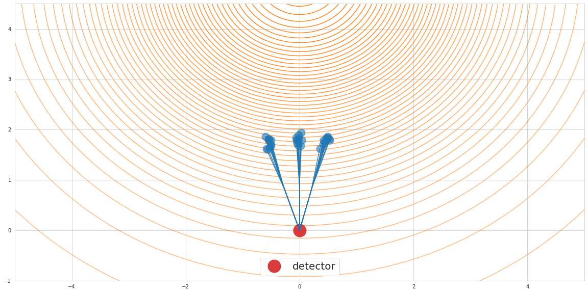
Figure 3.1: The contours correspond to level sets of the materials mixture with $\vartheta_{\mu}=\left(0,5\right)$ and $\vartheta_{\sigma}=\sqrt{10}$. In blue we show the BMC simulated trajectories. For the sake of simplicity, we assume the known particle flux is constant equals to one and is reached after two steps. The measurement angles on the detector have been arbitrarily chosen at $\left(-\frac{\pi}{5},0,\frac{4\pi}{25}\right)$.

If the parameters $\vartheta$ are fixed, the distribution of the flux approaches a normal one with mean estimated by:

$$\hat{\phi}(\textbf{s}_{f};\vartheta)=\frac{1}{N}\sum_{k=1}^{N}\omega_{k}(\vartheta)\cdot\phi(\textbf{s}_{i,k})$$ (3.2)

and variance $\sigma_{N}^{2}=\mathcal{O}(1/N)$ as the number of particles $N\rightarrow\infty$, which we treat as fixed for all purposes.

Let us postulate that the random error in our model follows a normal distribution $N(0,\sigma_{M}^{2})$. Taking a Bayesian approach, we give a normal distribution $\vartheta\sim N(\mu_{\vartheta},\sigma_{\vartheta}^{2})$ to the prior as well. Hence, the log-probability for observing a flux $\phi(\textbf{s}_{f})$ on the detector evaluates to:

$$\mathcal{L}(\vartheta)=-\frac{\|\phi(\textbf{s}_{f})-\hat{\phi}(\textbf{s}_{f};\vartheta)\|^{2}}{\sigma_{M}^{2}}-\frac{\|\vartheta-\mu_{\vartheta}\|^{2}}{\sigma_{\vartheta}^{2}}$$ (3.3)

up to a constant.

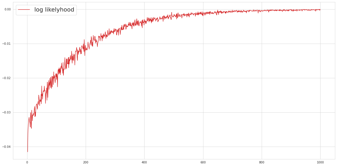
Figure 3.2: SGD convergence over 1000 steps with learning rate 0.05

Example 2.

We note that the routine backward_mc 4 is a differentiable program built on top of LibTorch’s Autograd library. It can be differentiated using torch::autograd::grad, which enables us to run a Stochastic Gradient Descent (SGD) optimisation to solve the inverse problem for $\vartheta$. This can be presented as a maximum likelihood estimation letting $\sigma_{\vartheta}\rightarrow\infty$.

Recalling figure 3.1, let us set $\bar{\vartheta}_{\mu}=\left(-1,5\right)$ and $\bar{\vartheta}_{\sigma}=\sqrt{10}$ as our true values and compute the observed flux for them. Taking out one measurement, at angle 0 say for validation later, we keep in the other two $\left(-\frac{\pi}{5},\frac{4\pi}{25}\right)$ for SGD.

Running the classical SGD update:

$$\vartheta\leftarrow\vartheta+\eta\nabla_{\vartheta}\mathcal{L}$$ (3.4)

starting from $\vartheta_{\mu}=\left(0,5\right)$ we obtain the convergence graph in figure 3.2. Taking the mean over the last 200 values we obtain the optimal parameters $\hat{\vartheta}_{\mu}=\left(-1.0033,4.9891\right)$ and $\hat{\vartheta}_{\sigma}^{2}=9.9611$ which are in good agreement with the true values $\bar{\vartheta}$ as expected. In future works, we will compare this approach against other reconstruction algorithms, with genuine dynamics from particle physics.

To close this section, we would like to demonstrate how one might explore further the fact that backward_mc 4 is a differentiable program.

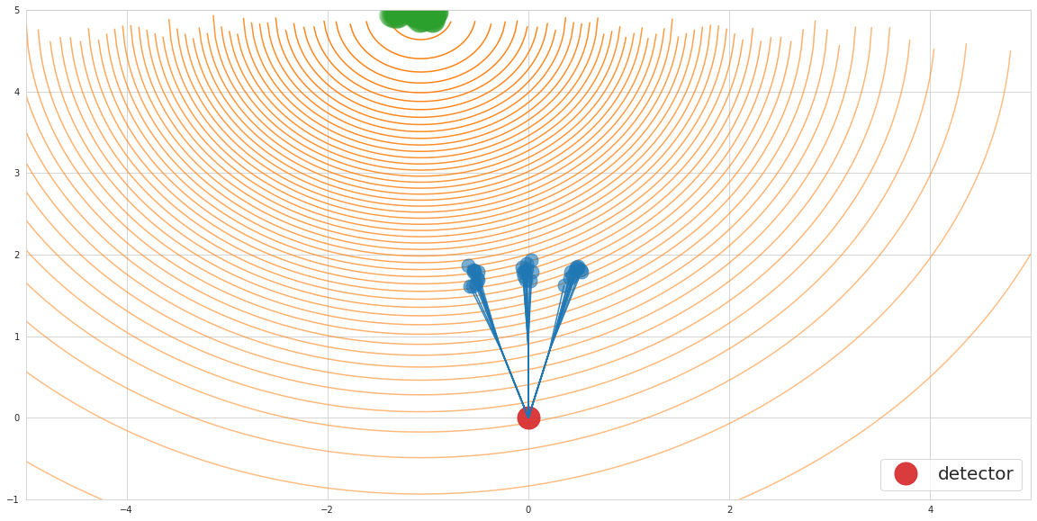
Figure 3.3: Optimal parameters and Bayesian Posterior sample

Example 3.

In example 2, we have left out from the optimisation the measurement at angle 0. We will use it to look at the stability of the optimal solution we found with Bayesian inference. For higher dimensional distributions exhibiting rough curvature standard Markov Chain Monte-Carlo schemes are not suitable. On has to rely on Hamiltonian Monte-Carlo (HMC) which uses Hamiltonian dynamics to build the MC chain.

The library NOA [1] implements Riemannian HMC with an explicit symplectic integrator as in [7], [5]. The Hamiltonian $H$ uses the log-probability density $\mathcal{L}(\vartheta)$ as potential, where $\vartheta\in\mathbb{R}^{d}$ denote the parameters which we augment with momentum coordinate $\chi\in\mathbb{R}^{d}$:

$$H(\vartheta,\chi)=\frac{1}{2}\chi^{t}M(\vartheta)^{-1}\chi+\frac{1}{2}\log\det(M(\vartheta))-\mathcal{L}(\vartheta).$$ (3.5)

Following M. Betancourt [2], the local metric is obtained applying a regularisation procedure in the form of the softabs map:

$$M=Q\cdot\lambda_{d}\coth(\alpha\lambda_{d})\cdot Q^{t}$$ (3.6)

where $Q(\vartheta),\lambda_{d}(\vartheta)$ stand for the eigendecomposition of $\nabla^{2}\mathcal{L}(\vartheta)$, and typically we set $\alpha=10^{6}$ for the softabs constant. Therefore, we are indirectly using the 3rd order derivative of our model for the flux.

This Hamiltonian is non-separable, and to avoid using an implicit integrator which is computationally heavy, one can rely on the explicit algorithm from M. Tao [12]. The phase space $\vartheta,\chi$ is augmented by $\vartheta^{*},\chi^{*}\in\mathbb{R}^{d}$ and we solve the corresponding separable Hamiltonian dynamics:

$$H^{*}(\vartheta,\chi,\vartheta^{*},\chi^{*})=H(\vartheta,\chi^{*})+H(\vartheta^{*},\chi)+\frac{1}{2}\Omega\cdot(\|\vartheta-\vartheta^{*}\|^{2}_{2}+\|\chi-\chi^{*}\|^{2}_{2})$$ (3.7)

where the constant $\Omega$ needs to be tuned.

We sample 300 points via the HMC scheme for $\mathcal{L}(\vartheta)$ defined using the reading at angle 0 only but with the prior mean given by the optimal solution found in example 2. The result is illustrated in figure 3.3. We reconfirm our result with a posterior sample mean $\hat{\vartheta}_{\mu}=\left(-1.0722,4.9530\right)\pm\left(0.1343,0.0410\right)$.

One important direction for improvement here is to introduce the appropriate form of Stochastic Gradient Riemannian HMC since the log-probability density is evaluated through backward MC.

4 Adjoint sensitivity methods

There is a challenge with the above approach differentiating through the MC simulation using AD. Our algorithm is not constant in the number of steps $n$ for the discretisation of the transport. This issue can be addressed by adjoint sensitivity methods [10].

Let us recall how this technique works for an ODE:

$$\frac{dx}{dt}=f(t,x(t),\vartheta).$$ (4.1)

Imagine that we want to compute the gradient of some scalar function:

$$\mathcal{L}(x(t_{1}))=\mathcal{L}\left(x(t_{0})+\int_{t_{0}}^{t_{1}}f(t,x(t),\vartheta)dt\right)$$ (4.2)

with respect to the parameters $\vartheta$.

An efficient way to tackle this task is to introduce the adjoint:

$$a(t)=\nabla_{x(t)}\mathcal{L}$$ (4.3)

which satisfies the adjoint ODE:

$$\frac{da}{dt}=-a(t)\cdot\nabla_{x}f(t,x(t),\vartheta).$$ (4.4)

The desired gradient is given then by a backward in time integral:

$$\nabla_{\vartheta}\mathcal{L}=-\int_{t_{1}}^{t_{0}}a(t)\cdot\nabla_{\vartheta}f(t,x(t),\theta)dt.$$ (4.5)

In our set-up, we are simulating the evolution back from the final state straightaway. Therefore, we can easily adapt the adjoint sensitivity method to the BMC scheme.

In doing so, we recall that the weight is computed iteratively:

$$\omega_{j+1}(\vartheta)=\frac{p_{\ell_{0}}(\textbf{s}_{j+1},\vartheta)}{p_{\ell_{0},b}(\textbf{s}_{j})}\det(\nabla_{\textbf{s}_{j}}\varphi_{j,\ell_{0}}^{-1})|_{x_{j,\ell_{0}}}\cdot\omega_{j}(\vartheta)$$ (4.6)

for $j=0..n-1$, with $\omega_{0}=1$ and $\omega_{n}$ giving the final weight.

The discrete adjoint sensitivity algorithm yielding $\mathcal{O}(1)$-memory derivative computations is simply obtained by differentiating through the above recursion:

$$\nabla_{\vartheta}^{m}\omega_{j+1}(\vartheta)=\det(\nabla_{\textbf{s}_{j}}\varphi_{j,\ell_{0}}^{-1})|_{x_{j,\ell_{0}}}\sum_{k=0}^{m}{m\choose k}\frac{\nabla_{\vartheta}^{k}p_{\ell_{0}}(\textbf{s}_{j+1},\vartheta)}{p_{\ell_{0},b}(\textbf{s}_{j})}\cdot\nabla_{\vartheta}^{m-k}\omega_{j}(\vartheta).$$ (4.7)

To evaluate $\nabla_{\vartheta}^{k}p_{\ell_{0}}$ one will still rely on the AD engine. However, the computational graph needed for reverse-mode differentiation can be freed after each step and executed in parallel for each particle.

The routine backward_mc_grad 5 in the appendix provides an implementation with first order derivative for the BMC scheme discussed in example 1.

5 Conclusion

In this paper, we have demonstrated how to efficiently integrate automatic differentiation and adjoint sensitivity methods with Backward Monte-Carlo schemes arising in the passage of particles through matter simulations.

We believe that this builds a whole new bridge between scientific machine learning and inverse problems arising in particle physics. In future, we hope to prove the success of this technique in a variety of image reconstruction problems with non-linear dynamics, starting with muography.

Acknowledgments

We would like to thank the MIPT-NPM lab and Alexander Nozik in particular for very fruitful discussions that have led to this work. We are very grateful to GrinisRIT for the support. This work has been initially presented in June 2021 at the QUARKS online workshops 2021 - “Advanced Computing in Particle Physics”.

Email: roland.grinis@grinisrit.com

Moscow Institute of Physics and Technology, Institutsky lane 9, Dolgoprudny, Moscow region, Russia, 141700

Appendix: Code examples

We have collected here the two BMC implementations for our basic example. You can reproduce all the calculations in this paper from the notebook differentiable_programming_pms.ipynb available in NOA [1].

For the specific code snippets here the only dependency is LibTorch:

⬇

#include <torch/torch.h>

The following routine will be used throughout and provides the rotations by a tensor angles for multiple scattering:

⬇

inline torch::Tensor rot(const torch::Tensor &angles)

{

const auto n = angles.numel();

const auto c = torch::cos(angles);

const auto s = torch::sin(angles);

return torch::stack({c, -s, s, c}).t().view({n, 2, 2});

}

Given the set-up in example 1 we define:

⬇

const auto detector = torch::zeros(2);

const auto materialA = 0.9f;

const auto materialB = 0.01f;

inline const auto PI = 2.f * torch::acos(torch::tensor(0.f));

inline torch::Tensor mix_density(

const torch::Tensor &states,

const torch::Tensor &vartheta)

{

return torch::exp(-(states - vartheta.slice(0, 0, 2))

.pow(2).sum(-1) / vartheta[2].pow(2));

}

Example 4.

This implementation relies completely on the AD engine for tensors. The whole trajectory is kept in memory to perform reverse-mode differentiation.

The routine accepts a tensor theta representing the angles for the readings on the detector, the tensor node encoding the mixture of the materials which is essentially our variable, and the number of particles npar.

It outputs the simulated flux on the detector corresponding to theta:

⬇

inline torch::Tensor backward_mc(

const torch::Tensor &theta,

const torch::Tensor &node,

const int npar)

{

const auto length1 = 1.f - 0.2f * torch::rand(npar);

const auto rot1 = rot(theta);

auto step1 = torch::stack({torch::zeros(npar), length1}).t();

step1 = rot1.matmul(step1.view({npar, 2, 1})).view({npar, 2});

const auto state1 = detector + step1;

auto biasing = torch::randint(0, 2, {npar});

auto density = mix_density(state1, node);

auto weights =

torch::where(biasing > 0,

(density / 0.5) * materialA,

((1 - density) / 0.5) * materialB) *

torch::exp(-0.1f * length1);

const auto length2 = 1.f - 0.2f * torch::rand(npar);

const auto rot2 = rot(0.05f * PI * (torch::rand(npar) - 0.5f));

auto step2 =

length2.view({npar, 1}) * step1 / length1.view({npar, 1});

step2 = rot2.matmul(step2.view({npar, 2, 1})).view({npar, 2});

const auto state2 = state1 + step2;

biasing = torch::randint(0, 2, {npar});

density = mix_density(state2, node);

weights *=

torch::where(biasing > 0,

(density / 0.5) * materialA,

((1 - density) / 0.5) * materialB) *

torch::exp(-0.1f * length2);

// assuming the flux is known equal to one at state2

return weights;

}

Example 5.

This routine adopts the adjoint sensitivity algorithm to earlier example 4. It outputs the value of the flux and the first order derivative w.r.t. the tensor node:

⬇

inline std::tuple<torch::Tensor, torch::Tensor> backward_mc_grad(

const torch::Tensor &theta,

const torch::Tensor &node)

{

const auto npar = 1; //work with single particle

auto bmc_grad = torch::zeros_like(node);

const auto length1 = 1.f - 0.2f * torch::rand(npar);

const auto rot1 = rot(theta);

auto step1 = torch::stack({torch::zeros(npar), length1}).t();

step1 = rot1.matmul(step1.view({npar, 2, 1})).view({npar, 2});

const auto state1 = detector + step1;

auto biasing = torch::randint(0, 2, {npar});

auto node_leaf = node.detach().requires_grad_();

auto density = mix_density(state1, node_leaf);

auto weights_leaf = torch::where(biasing > 0,

(density / 0.5) * materialA,

((1 - density) / 0.5) * materialB) * torch::exp(-0.01f * length1);

bmc_grad += torch::autograd::grad({weights_leaf}, {node_leaf})[0];

auto weights = weights_leaf.detach();

const auto length2 = 1.f - 0.2f * torch::rand(npar);

const auto rot2 = rot(0.05f * PI * (torch::rand(npar) - 0.5f));

auto step2 = length2.view({npar, 1}) * step1 / length1.view({npar, 1});

step2 = rot2.matmul(step2.view({npar, 2, 1})).view({npar, 2});

const auto state2 = state1 + step2;

biasing = torch::randint(0, 2, {npar});

node_leaf = node.detach().requires_grad_();

density = mix_density(state2, node_leaf);

weights_leaf = torch::where(biasing > 0,

(density / 0.5) * materialA,

((1 - density) / 0.5) * materialB) * torch::exp(-0.01f * length2);

const auto weight2 = weights_leaf.detach();

bmc_grad = weights * torch::autograd::grad({weights_leaf}, {node_leaf})[0]

+ weight2 * bmc_grad;

weights *= weight2;

// assuming the flux is known equal to one at state2

return std::make_tuple(weights, bmc_grad);

}

References

- [1] Differentiable Programming for Optimisation Algorithms over LibTorch. https://github.com/grinisrit/noa
- [2] M. Betancourt. A general metric for Riemannian manifold Hamiltonian Monte Carlo. International Conference on Geometric Science of Information, Springer, 327-334, 2013.
- [3] L. Capriotti and M. B. Giles. Algorithmic differentiation: Adjoint greeks made easy. SSRN Electronic Journal, 2011.
- [4] R. T. Q. Chen, Y. Rubanova, J. Bettencourt, and D. K. Duvenaud. Neural ordinary differential equations. Advances in neural information processing systems, 6571-6583, 2018.
- [5] A. Cobb, A. Baydin, A. Markham, and S. Roberts. Introducing an explicit symplectic integration scheme for Riemannian manifold Hamiltonian Monte-Carlo. preprint arXiv:1910.06243, 2019.
- [6] L. Desorgher, F. Lei, and G. Santin. Implementation of the reverse/adjoint Monte Carlo method into Geant4. Nucl. Instrum. Meth., A621:247-257, 2010.
- [7] M. Girolami and B. Calderhead. Riemann manifold Langevin and Hamiltonian Monte Carlo methods. Journal of the Royal Statistical Society Series B, 73(2):123-214, 2011.
- [8] X. Li, T.-K. L. Wong, R. T. Q. Chen, and D. K. Duvenaud. Scalable gradients for stochastic differential equations International Conference on Artificial Intelligence and Statistics, 2020
- [9] V. Niess, A. Barnoud, C. Carloganu, and E. Le Menedeu. Backward Monte-Carlo applied to muon transport. Comput. Phys. Comm., 229(54), 2018.
- [10] L. S. Pontryagin, E. F. Mishchenko, V. G. Boltyanskii, and R. V. Gamkrelidze. The mathematical theory of optimal processes. John Wiley S., New York, London, 1962.
- [11] C. Rackauckas, Y. Ma, J. Martensen, C. Warner, K. Zubov, R. Supekar, D. Skinner, and A. Ramadhan. Universal differential equations for scientific machine learning. preprint arXiv:2001.04385, 2020.
- [12] M. Tao. Explicit high-order symplectic integrators for charged particles in general electromagnetic fields. J. of Comp. Phys., 327:245-251, 2016.