Some unusual wormholes in general relativity

K. A. Bronnikov
Center for Gravitation and Fundamental Metrology, VNIIMS, Ozyornaya ul. 46, Moscow 119361, Russia;
Institute of Gravitation and Cosmology, Peoples’ Friendship University of Russia (RUDN University),
         ul. Miklukho-Maklaya 6, Moscow 117198, Russia;
National Research Nuclear University “MEPhI”, Kashirskoe sh. 31, Moscow 115409, Russia

In this short review we present some recently obtained traversable wormhole models in the framework of general relativity (GR) in four and six dimensions that somehow widen our common ideas on wormhole existence and properties. These are, first, rotating cylindrical wormholes, asymptotically flat in the radial direction and existing without exotic matter. The topological censorship theorems are not violated due to lack of asymptotic flatness in all spatial directions. Second, these are cosmological wormholes constructed on the basis of the Lemaître-Tolman-Bondi solution. They connect two copies of a closed Friedmann world filled with dust, or two otherwise distant parts of the same Friedmann world. Third, these are wormholes obtained in six-dimensional GR, whose one entrance is located in “our” asymptotically flat world with very small extra dimensions while the other “end” belongs to a universe with large extra dimensions and therefore different physical properties. The possible observable features of such wormholes are briefly discussed.

1 Introduction

Wormhole physics has become quite a popular research area, even though nobody has ever seen a real wormhole in Nature. Thus, on August 1, 2021, a search for the term “wormhole” on the site arxiv.org gave 2,154 results for all years and 303 results for past 12 months. This popularity looks natural since a wormhole is one more, in addition to a black hole, and even simpler manifestation of a strongly curved space-time which can lead to many effects of great interest.

The term “wormhole” is multi-valued: while it originally means a kind of tunnel or shortcut between different space-times or between otherwise distant regions of the same space-time (it is also called a Lorentzian wormhole), many authors discuss what they call quantum and Euclidean wormholes, giving this name to wave functions or objects in spaces with Euclidean signature whose properties resemble those of “tunnels”. They are not our subject here. Among Lorentzian wormholes, one often speaks of traversable or nontraversable ones, and some of them can also be one-way traversable. A lack of two-way traversability is generally caused by the existence of horizons, and, in my opinion,  it is then more correct to call such objects black holes thus avoiding their confusion with wormholes. Curiously, the first mentions of wormhole-like geometries (though, purely spatial ones) by Flamm [1] and by Einstein and Rosen [2] actually referred to the Schwarzschild and Reissner-Nordström black hole space-times. In this paper we are going to discuss only two-way traversable wormholes without indicating this each time.

Another issue is that of “unusual” wormholes. Which of them could be called “usual” if none have been observed as yet? The answer is — those which are most frequently discussed, hence, spherically or axially symmetric ones, possibly with rotation, connecting spatial regions with similar properties, those which are most frequently asymptotically flat or asymptotically AdS and, if considered in the framework of GR, necessarily require for their support some kind of exotic (or phantom) matter, violating the Null Energy Condition (NEC), a part of the Weak Energy Condition (WEC) that provides nonnegativity of the energy density in any reference frame. In GR extensions, the role of exotic matter may be implemented by some geometric quantities like torsion, nonmetricity or nonlinear curvature constructs, maybe of extra-dimensional origin. There are many interesting tasks and problems on this trend, connected with their possible observable features, their stability, evolution, etc., see, e.g., the reviews [3, 4, 5], but we will leave them aside in the present paper.

One kind of “unusual” wormholes to be discussed here is connected with topological features that make impossible asymptotic flatness in all spatial directions: these are cylindrically symmetric configurations, looking like cosmic strings when observed from afar. It turns out that this structure allows one to avoid the well-known topological censorship theorems [6, 7] and to construct stationary wormhole models in GR without WEC violation [8, 9, 10].

Other wormholes of interest are those cosmological in nature: they exist in the framework of cosmological models and may be, above all, relevant to early Universe descriptions, for example, those with two de Sitter asymptotic regions may connect otherwise distant parts of an inflationary Universe [11], thus increasing its causal connection. We, however, focus here on the recent and somewhat unexpected inference [12, 13] that cosmological wormholes may be supported by evolving dust distributions and obtained based on the Lemaître-Tolman-Bondi (LTB) famous solution [14, 15, 16].

Lastly, among the diverse wormhole models in multidimensional gravity theories, we will single out and discuss a curious class of wormholes in six-dimensional (6D) GR [17, 18] able to connect our 4D space-time possessing small and invisible extra dimensions with another one, where the extra dimensions are large, or maybe with a multidimensional region of our own Universe if such regions do exist.

Sections 2–4 are devoted to these three kinds of unusual wormholes, and Section 5 is a conclusion.

2 Cylindrical symmetry and phantom-free models

An important topological censorship theorem [6] asserts that in GR, if an asymptotically flat, globally hyperbolic space-time (${\mathbb{M}},g_{\mu\nu}$) satisfies the averaged NEC, then every causal curve from past null infinity to future null infinity is homotopic to a topologically trivial curve of this kind. As a consequence, if there emerges a wormhole-like structure, it cannot be traversed even by light, to say nothing on massive bodies, probably due to a rapid collapse of such an object. Somewhat weaker versions of this theorem concern static wormholes, proving the necessity of NEC violation at wormhole throats, i.e., their narrowest parts [19, 20].

Is it possible to circumvent these theorems? A straightforward way of obtaining wormhole solutions in GR is to violate the NEC by introducing some kind of exotic or phantom matter, for example, a scalar field with negative kinetic energy or thin shells, as is done in a lot of studies. One can also recall such axially symmetric wormhole structures in GR as the Kerr metric with a supercritical angular momentum, Zipoy’s static solutions [21], their extensions with electromagnetic and scalar fields [22, 23, 24]: each of them connects two different flat infinities, being free from exotic matter but, instead, containing a naked ring singularity around a disk-shaped throat, thus violating global hyperbolicity.

One more way to phantom-free wormholes is to replace GR with some extended theory of gravity, delegating the role of exotic matter to geometric quantities like torsion or the Gauss-Bonnet invariant, see the reviews [3, 4, 5].

Let us. however, discuss the fourth way: remaining in the framework of GR, we abandon asymptotic flatness in all directions, assuming, in the simplest case, cylindrical symmetry. To describe a stringlike object observable from a weakly curved region of space, a cylindrical metric should be asymptotically flat in the radial directions, whereas in the longitudinal direction the curvature does not change and remains arbitrarily large.

2.1 Definitions of a cylindrical wormhole

A stationary cylindrically symmetric space-time can be described by the metric

$$ds^{2}={\rm\,e}^{2\gamma(x)}[dt-E(x){\rm\,e}^{-2\gamma(x)}\,d\varphi]^{2}-{\rm\,e}^{2\alpha(x)}dx^{2}-{\rm\,e}^{2\mu(x)}dz^{2}-{\rm\,e}^{2\beta(x)}d\varphi^{2},$$ (1)

where $x$, $z\in{\mathbb{R}}$ and $\varphi\in[0,2\pi)$ are the radial, longitudinal and angular coordinates, respectively, and $x$ is specified up to a substitution $x\to f(x)$, hence its range depends both on its choice (“gauge”) and on the geometry under consideration. The quantity $r(x)={\rm\,e}^{\beta}$ is the circular radius, whose possible regular minimum can be identified as a wormhole throat (a so-called “r-throat”).

There is an alternative definition of a throat (an “a-throat”) as a regular minimum of the “area function” $a(x)={\rm\,e}^{\beta+\mu}$, but it is in general less applied since $r(x)$ is more evident. Also, if the whole configuration is asymptotically flat at large radii on both ends of the $x$ range, it evidently means that there are throats according to both definitions. Therefore we will pay attention to both of them.

The off-diagonal metric component $E$ describes rotation, unless $E{\rm\,e}^{-2\gamma}={\rm const}$; in the latter case the metric is static, and $E=0$ is easily obtained by redefining the time coordinate ($t\mapsto t+{\rm const}\cdot\varphi$).

A wormhole with the metric (1) may be defined as a regular space-time region with finite functions $\alpha,\beta,\gamma,\mu,E$, containing a throat $x=x_{\rm th}$ (by one or both of the above definitions), and such that the radius $r(x)$ and/or the area function $a(x)$ reach values much larger than at $x=x_{\rm th}$ on both sides of the throat.

2.2 A static wormhole with a magnetic field source

It is not a problem to find solutions to the Einstein equations with r-throats and non-phantom sources. One such example is a static solution ($E=0$) with an azimuthal magnetic field [25, 26, 27] written in terms of the harmonic radial coordinate $x$ satisfying the gauge condition $\alpha=\beta+\gamma+\mu$:

$${}ds^{2}=\frac{q^{2}\cosh^{2}kx}{k^{2}}\Big{[}e^{2a}dt^{2}-e^{2(a+b)x}dx^{2}-e^{2bx}d\phi^{2}\Big{]}-\frac{k^{2}dz^{2}}{q^{2}\cosh^{2}kx},$$

$${}q,a,b,k={\rm const}>0;\qquad ab=k^{2};$$

$${}F^{xz}=q{\rm\,e}^{-2\alpha(x)},\qquad F_{xz}=q{\rm\,e}^{2\mu(z)};\qquad B^{2}=q^{2}{\rm\,e}^{2\mu-2\alpha}=\frac{k^{4}{\rm\,e}^{-2(a+b)x}}{q^{2}\cosh^{4}kx},$$ (2)

where $x\in{\mathbb{R}}$, $F_{\mu\nu}$ is the electromagnetic field tensor, and $B$ is the $\varphi$-directed magnetic induction created by an effective current $q$ along the $z$ axis, The solution (2.2) describes a wormhole if $a>k$ since in this case $r={\rm\,e}^{\beta}\to\infty$ at both ends, $x\to\pm\infty$. The wormhole is highly asymmetric, for example, $B\to 0$ at the right end ($x\to\infty$) and to infinity at the left end, from which it is clear that $x\to-\infty$ is a singularity. Meanwhile, we have ${\rm\,e}^{\mu}\to 0$ (a shrinking longitudinal scale) on both ends. Moreover, the area function $a(x)={\rm\,e}^{\beta+\mu}={\rm\,e}^{bx}$ has no minimum, and (2.2) is a wormhole solution only by the definition related to $r(x)$.

2.3 A rotating wormhole with a scalar field source

Another example is a rotating cylindrical wormhole with a massless scalar field $\phi$ [28] having the Lagrangian $L_{\phi}={\tfrac{1}{2}}\varepsilon\phi^{,\mu}\phi_{,\mu}$, where $\varepsilon=+1$ corresponds to a canonical scalar field, and $\varepsilon=-1$ to a phantom one. In terms of the metric (1) and the harmonic radial coordinate $x$, the solution reads

$${}{\rm\,e}^{2\alpha}={\rm\,e}^{(4m-2h)x},\qquad\qquad{\rm\,e}^{2\beta}=\frac{k{\rm\,e}^{2hx}}{2\omega_{0}\sin kx},$$

$${}{\rm\,e}^{2\gamma}=\frac{2\omega_{0}}{k}{\rm\,e}^{2hx}\sin kx,\qquad{\rm\,e}^{2\mu}={\rm\,e}^{-2mx},\qquad\phi=Cx,$$

$${}E=\frac{{\rm\,e}^{2hx}}{k}\big{[}E_{0}\sin kx+k\cos kx\big{]},\qquad\omega=\omega_{0}{\rm\,e}^{-\mu-2\gamma}=\frac{k{\rm\,e}^{(m-2h)x}}{2\sin kx},$$ (3)

where $\omega$ is the vorticity defined as the angular velocity of tetrad rotation [29], while $C,h,k,m,E_{0}$ and $\omega_{0}$ are integration constants related by

$$k^{2}=4h(2m-h)-2\kappa\varepsilon C^{2},$$ (4)

where $\kappa=8\pi G$ is the gravitational constant.

The range of the coordinate $x$ in (2.3) is $x\in(0,\pi)$, and its both extremes possess $r(x)={\rm\,e}^{\beta}\to\infty$ and $a(x)={\rm\,e}^{\beta+\mu}\to\infty$, but the metric is singular there due to $g_{tt}={\rm\,e}^{2\gamma}\to 0$. It can also be noticed that this wormhole solution exists with both phantom and canonical scalar fields ($\varepsilon=\pm 1$) and even in the vacuum case ($C=0\ \Rightarrow\ \phi=0$).

It is known, however, that to support a static cylindrical wormhole with an a-throat, its matter source should necessarily violate the WEC and NEC [26]. Hence it is rotation that provides the wormhole nature of (2.3).

2.4 The rotational part of Ricci and Einstein tensors

To explain why rotation favours the emergence of wormholes, let us assume that the matter source of the metric (1) is taken in its comoving reference frame, in particular, its velocity in the $\varphi$ direction is zero. Then we can directly integrate the Einstein equation $R^{3}_{0}\propto(\omega{\rm\,e}^{2\gamma+\mu})^{\prime}=0$ (the prime stands for $d/dx$) to obtain $\omega=\omega_{0}{\rm\,e}^{-\mu-2\gamma}$ with $\omega_{0}={\rm const}$. Then the nonzero components of the Ricci tensor for the metric (1) have the form

$$R^{0}_{0} = -{\rm\,e}^{-2\alpha}[\gamma^{\prime\prime}+\gamma^{\prime}(\sigma^{\prime}-\alpha^{\prime})]-2\omega^{2},$$

$${}R^{1}_{1} = -{\rm\,e}^{-2\alpha}[\sigma^{\prime\prime}+\sigma^{\prime}{}^{2}-2U-\alpha^{\prime}\sigma^{\prime}]+2\omega^{2},$$

$${}R^{2}_{2} = -{\rm\,e}^{-2\alpha}[\mu^{\prime\prime}+\mu^{\prime}(\sigma^{\prime}-\alpha^{\prime})],$$

$${}R^{3}_{3} = -{\rm\,e}^{-2\alpha}[\beta^{\prime\prime}+\beta^{\prime}(\sigma^{\prime}-\alpha^{\prime})]+2\omega^{2},$$

$${}R^{0}_{3} = G^{0}_{3}=E{\rm\,e}^{-2\gamma}(R^{3}_{3}-R^{0}_{0}),$$ (5)

under an arbitrary choice of the coordinate $x$, with the notations

$$\sigma=\beta+\gamma+\mu,\qquad U=\beta^{\prime}\gamma^{\prime}+\beta^{\prime}\mu^{\prime}+\gamma^{\prime}\mu^{\prime}.$$ (6)

We see that the rotational parts of the Ricci tensor and the Einstein tensor $G_{\mu}^{\nu}=R_{\mu}^{\nu}-{\tfrac{1}{2}}\delta_{\mu}^{\nu}R$ are separated from their static parts, corresponding to (1) with $E\equiv 0$:

$${}R_{\mu}^{\nu}=R_{\mu}^{\nu}{}_{\rm(st)}+R_{\mu}^{\nu}{}_{\rm(rot)},\qquad R_{\mu}^{\nu}{}_{\rm(rot)}=\omega^{2}\mathop{\rm diag}\nolimits(-2,2,0,2),$$

$${}G_{\mu}^{\nu}=G_{\mu}^{\nu}{}_{\rm(st)}+G_{\mu}^{\nu}{}_{\rm(rot)},\qquad G_{\mu}^{\nu}{}_{\rm(rot)}=\omega^{2}\mathop{\rm diag}\nolimits(-3,1,-1,1).$$ (7)

In the Einstein equations $G_{\mu}^{\nu}=-\kappa T_{\mu}^{\nu}$, the stress-energy tensor (SET) $T_{\mu}^{\nu}$ thus actually acquires quite an exotic contribution $G_{\mu}^{\nu}{}_{\rm rot}/\kappa$ due to rotation, with negative effective energy density equal to $-3\omega^{2}/\kappa$.

2.5 How to obtain asymptotically flat rotating wormholes

If our aim is to obtain phantom-free cylindrical wormholes which could be observable from weakly curved regions of space on each side from the throat, we should require their asymptotic flatness in the radial direction at both ends of the $x$ range. We have seen that it is impossible with static wormholes due to conditions on an a-throat. Rotation allows for more or less easily finding solutions with both kinds of throats, but it becomes quite a hard problem to obtain asymptotic flatness. The following trick was suggested in [28] to overcome this difficulty: having obtained a phantom-free cylindrical wormhole solution, cut out from it a regular region containing the throat and join it to two flat regions extended to infinity on each side from the throat. The whole system will thus become twice asymptotically flat and potentially observable from each side. To form a single space-time in this way, the external and internal metrics on the two junction surfaces $\Sigma_{+}$ and $\Sigma_{-}$ should be identified, but the derivatives of the metric in the direction across $\Sigma_{+}$ and $\Sigma_{-}$ — that is, in the radial direction — will in general suffer discontinuities, which, according to the Darmois-Israel formalism [30, 31], mean that there are some surface matter distributions on $\Sigma_{\pm}$. Then, to obtain a completely phantom-free wormhole model, we should require that this surface matter should satisfy the WEC (and NEC as its part).

The first attempts to realize this program were undertaken in [28] using rotating wormhole solutions with scalar fields with or without self-interaction potentials. With such interior solutions, it turned out to be impossible to satisfy the WEC on both surfaces $\Sigma_{p}m$. Later on, a no-go theorem was proved [32], claiming that the threefold construction described above cannot be phantom-free if the SET of matter in the internal (wormhole) region satisfies the equality $T^{t}_{t}=T^{z}_{z}$. This equality holds for all kinds of scalar fields $\phi(x)$ minimally coupled to gravity, for example, those of generalized k-essence type, with an arbitrary Lagrangian of the form $L(\phi,X)$ with $X=g^{\mu\nu}\phi_{,\mu}\phi_{,\nu}$.

Successful models of this kind were obtained later in [8] with a wormhole solution sourced by a certain kind of anisotropic fluid, in [9] with an isotropic maximally stiff perfect fluid with the equation of state $p=\rho$, and in [10] with a source consisting of a perfect fluid with $p=w\rho$ ($|w|<1$), and a magnetic field along the $z$ axis whose source is a circular electric current in the angular direction. The model of [10] tends to that of [9] in the limit $w\to 1$, while in the same limit the azimuthal current and the magnetic field vanish. In the next subsection we briefly describe the model of [9].

2.6 An asymptotically flat rotating wormhole model with stiff matter

In a perfect fluid with the equation of state $p=\rho$, the speed of sound is equal to the speed of light, which greatly simplifies the equations of motion and has led to obtaining numerous solutions which are either unique or much simpler than their counterparts with other equations of state: see, e.g., [33, 27] for a general exposition, [34, 35, 36, 37] for static solutions, [38] for wavy ones, and [39, 40, 41, 42, 43] for stationary ones; applications of stiff matter in modern theoretical cosmology can also be mentioned, see, e.g., [44, 45]; see also references therein.

As before, let us use the Einstein equations for the metric (1) with the harmonic radial coordinate, $\alpha=\beta+\gamma+\mu$. For matter density, the conservation law gives $\rho=\rho_{0}{\rm\,e}^{-2\gamma}$. Furthermore, one of the equations reads simply

$$\mu^{\prime\prime}=0\ \ \Rightarrow\ \ \mu=mx+\mu_{0},\hskip 28.45274ptm,\mu_{0}={\rm const},$$ (8)

and we put $\mu_{0}=0$ by properly rescaling the $z$ axis. Other equations then imply

$$\beta^{\prime\prime}=2\omega_{0}^{2}{\rm\,e}^{2\beta-2\gamma},\hskip 28.45274pt\beta^{\prime\prime}+\gamma^{\prime\prime}=2\kappa\rho_{0}{\rm\,e}^{2\beta+2mx}.$$ (9)

For simplicity let us assume symmetry under reflections $x\to-x$, so that $m=0$, and $\gamma\equiv 0$. We then obtain

$$\beta^{\prime\prime}=2\omega_{0}^{2}{\rm\,e}^{2\beta},\hskip 28.45274pt\kappa\rho_{0}=\omega_{0}^{2}.$$ (10)

From the three branches of solutions to the Liouville equation for $\beta$, we choose the one where the function $\beta(x)$ has a minimum, necessary for obtaining a wormhole solution. We thus have

$${\rm\,e}^{\beta}=\frac{k}{\sqrt{2\omega_{0}^{2}}\cos(kx)},\hskip 28.45274ptk={\rm const}>0,\hskip 28.45274ptx\in(-\pi/2,\pi/2)$$ (11)

under a proper choice of the zero point of $x$. It remains to find $E(x)$, and to do that we use the expression following from the definition of $\omega(x)$ in terms of $E$ and the expression of $\omega(x)$ implied by the assumed comoving nature of the reference frame (see, e.g, [28, 9]):

$$\omega(x)={\dfrac{1}{2}}(E{\rm\,e}^{-2\gamma})^{\prime}{\rm\,e}^{\gamma-\beta-\alpha}=\omega_{0}{\rm\,e}^{-\mu-2\gamma}$$ (12)

As a result, we have

$$E=2\omega_{0}{\rm\,e}^{2\gamma}\int{\rm\,e}^{\alpha+\beta-\mu-3\gamma}dx=\frac{1}{\omega_{0}}\int\frac{k^{2}dx}{\cos^{2}(kx)}=\frac{k}{\omega_{0}}\tan(kx),$$ (13)

where we have chosen the integration constant so that $E(x)$ is an odd function, it is convenient for the subsequent matching with the exterior Minkowski metric. For the same purpose we introduce an arbitrary time scale by putting $dt\mapsto\sqrt{P}d\tau$, $P={\rm const}>0$. We also have $\kappa\rho_{0}=\omega_{0}^{2}$.

Thus we know the solution completely. It is most conveniently expressed in terms of a new radial coordinate, $y=k\tan(kx)$:

$$dx=\frac{dy}{k^{2}+y^{2}},\qquad{\rm\,e}^{2\beta}=\frac{k^{2}+y^{2}}{2\omega_{0}^{2}},\qquad E=\frac{\sqrt{P}y}{\omega_{0}},$$ (14)

and consequently

$$ds^{2}=\bigg{(}\sqrt{P}dt-\frac{y}{\omega_{0}}d\varphi\bigg{)}^{2}-\frac{dy^{2}}{2\omega_{0}^{2}(k^{2}+y^{2})}-dz^{2}-(k^{2}+y^{2})\frac{d\varphi^{2}}{2\omega_{0}^{2}}.$$ (15)

The solution is regular at all $y\in{\mathbb{R}}$, and a minimum of $r(x)$ occurs at $y=0$. One can notice, however, that at $y^{2}>k^{2}$ it becomes $g_{33}>0$, so that the coordinate circles $0<\phi<2\pi$ are closed timelike curves, violating causality.

Having obtained this wormhole solution, let us try to match it at some values of $y$, both positive and negative, to the Minkowski metric, taken in a rotating reference frame:

$$ds_{\rm M}^{2}=dt^{2}-dX^{2}-dz^{2}-X^{2}(d\varphi+\Omega dt)^{2},$$ (16)

so that in the notations of (1) we have

$${}{\rm\,e}^{\alpha}=1,\qquad{\rm\,e}^{2\gamma}=1-\Omega^{2}X^{2},\qquad{\rm\,e}^{2\beta}=\frac{X^{2}}{1-\Omega^{2}X^{2}},\qquad E=\Omega X^{2},\qquad\omega=\frac{\Omega}{1-\Omega^{2}X^{2}},$$

$${}\gamma^{\prime}=-\frac{\Omega X}{1-\Omega^{2}X^{2}},\qquad\mu^{\prime}=0,\qquad\beta^{\prime}=\frac{1}{X}+\frac{\Omega^{2}X}{1-\Omega^{2}X^{2}}.$$ (17)

If we identify a surface $y=y_{0}$ in the wormhole space-time (15) with a surface $X=X_{0}$ in (16), the matching conditions are

$$[\beta]=0,\quad[\mu]=0,\quad[\gamma]=0,\quad[E]=0,$$ (18)

where, as usual, for any $f(x)$, $[f]$ denotes its jump at the junction $\Sigma$. With (18), the coordinates $t,z,\phi$ can be identified in the whole space. The choice of the radial coordinates may be different on different sides from $\Sigma$, but it is unimportant since all quantities involved in the matching conditions are insensitive to this coordinate choice.

The junction surface $\Sigma$ having been identified, we can determine its material content using the Darmois-Israel formalism [30, 31, 46]: its SET $S_{a}^{b}$ is found in terms of the extrinsic curvature $K_{a}^{b}$ as

$${}S_{a}^{b}=\kappa^{-1}[\tilde{K}_{a}^{b}],\qquad\tilde{K}_{a}^{b}:=K_{a}^{b}-\delta_{a}^{b}K^{c}_{c},$$ (19)

where $a,b,c=0,2,3$. The WEC requirements for the surface SET read

$$S_{00}/g_{00}=\sigma_{s}\geq 0,\qquad\ S_{ab}\xi^{a}\xi^{b}\geq 0,$$ (20)

where $\sigma_{s}$ is the surface energy density and $\xi^{a}$ an arbitrary null vector on $\Sigma$. As shown in [8, 9], the requirements (20) reduce to

$$a+c+\sqrt{(a-c)^{2}+4d^{2}} \geq 0,$$ (21)

$$a+c+\sqrt{(a-c)^{2}+4d^{2}}+2b \geq 0,$$ (22)

$$a+c \geq 0,$$ (23)

with

$$a=\big{[}{\rm\,e}^{-\alpha}(\beta^{\prime}+\mu^{\prime})\big{]},\qquad b=\big{[}{\rm\,e}^{-\alpha}(\beta^{\prime}+\gamma^{\prime})\big{]},\qquad c=\big{[}{\rm\,e}^{-\alpha}(\gamma^{\prime}+\mu^{\prime})\big{]},\qquad d=-[\omega],$$ (24)

where the prime denotes a derivatives in the radial coordinate used in the corresponding spatial region.

Let us apply these conditions, beginning, for certainty, with the surface $\Sigma_{+}$ ($y=y_{0}>0$, $X=X_{0}>0$). The condition $[\mu]=0$ is trivial, while the other three conditions (18) give

$$P=1-\Omega^{2}X^{2},\hskip 28.45274pt\Omega X^{2}=\frac{y\sqrt{P}}{\omega_{0}},\hskip 28.45274pt\frac{k^{2}+y^{2}}{2\omega_{0}^{2}}=\frac{X^{2}}{P}.$$ (25)

where the index “zero” at $X$ and $y$ is omitted with no risk of confusion, and we assume $\omega_{0}>0$. There are initially six independent parameters [$P,k,\omega_{0},y$ in the internal metric (15) and $\Omega,X$ in (16)], and they are connected by three conditions (25). We can choose the following independent parameters: $X=X_{0}$ with the dimension of length (specifying the length scale of the model), and the dimensionless $y=y_{0}$ and $P$, then for the remaining parameters we obtain:

$$\Omega=\frac{\sqrt{1-P}}{X},\hskip 28.45274pt\omega_{0}=\frac{\sqrt{P}y}{\sqrt{1-P}X},\hskip 28.45274ptk^{2}=y^{2}\frac{1+P}{1-P},$$ (26)

which leads to the following expressions for the quantities $a,b,c,d$ from (21):

$${}a=\frac{P^{3/2}y-1}{PX},\qquad b=\frac{1-y\sqrt{P}}{X},\qquad c=\frac{P-1}{PX},\qquad d=\frac{\sqrt{P}y-1+P}{XP\sqrt{1-P}}.$$ (27)

Ignoring the common factor $1/X$, it is straightforward to verify that the requirements (21), (22), (23) are fulfilled under the condition

$$y\geq\frac{2-P}{P^{3/2}}.$$ (28)

Now let us discuss the same requirements on $\Sigma_{-}$, specified by $X=-X_{0}<0$ and $y=-y_{0}<0$. In all expressions (27) the factor $1/X$ is now negative. But, at the same time, the signs of all discontinuities also change: on $\Sigma_{+}$ we took $[f]=f_{\rm out}-f_{\rm in}$ for every quantity $f$, whereas on $\Sigma_{-}$ the opposite must be taken. As a result, the parameters $a,b,c$ preserve their form (27) with $X$ replaced by $|X|$ (where we denote $y=|y_{0}|>0$). For $d=-[\omega]$ we must bear in mind that, by (25), $\Omega(\Sigma_{-})=-\Omega(\Sigma_{+})$, whereas in the internal solution $\omega(\Sigma_{-})=\omega(\Sigma_{+})$, therefore, on $\Sigma_{-}$

$$d\ \mapsto\ d_{-}=-\frac{1-P+|y|\sqrt{P}}{|X|P\sqrt{1-P}},$$

so that $|d_{-}|>|d|$, making it even easier to fulfill the requirement (22). Thus all WEC requirements are fulfilled under the same condition (28), and so this condition leads to a completely phantom-free wormhole model.

Moreover, from (26) it follows $y_{0}^{2}<k^{2}$, hence $y^{2}<k^{2}$ in the whole internal region, therefore closed timelike curves are absent. For $P\in(0,1)$, according to (28), the parameters $y=y_{0}$ and $k$ should be large enough, see Fig. 1.

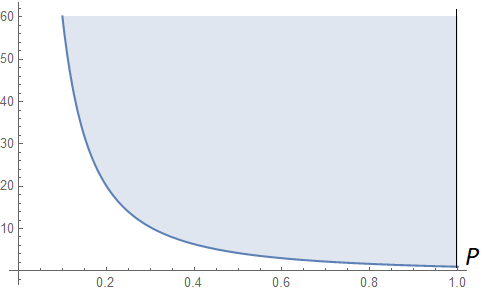
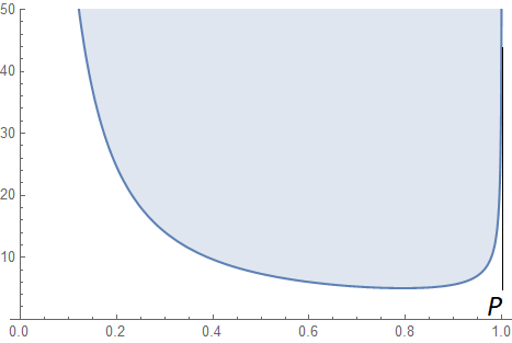
Figure 1: Admissible values of the parameters $y_{0}$ (left panel) and $k$ (right panel) in our wormhole model are shown by gray areas.

The model described, though quite simple, looks rather artificial, but the very existence of such models proves an important statement: it is possible to obtain phantom-free wormholes in the framework of GR, but at the expense of lacking asymptotic flatness in all directions. Other models of this kind have been constructed in [8, 10].

To describe the external regions of cylindrical wormholes, we have been using the Minkowski metric in the form (16). In the same way, we can consider, instead, a cosmic string metric: to do so, it is sufficient to replace $X$ in all equations with $X\sqrt{1-{\tilde{\alpha}}/(2\pi)}$, where the angular deficit $\tilde{\alpha}$ is interpreted as resulting from an effective linear density $\tilde{\mu}$ of the cosmic string [47], $\tilde{\alpha}=16\pi^{2}G\tilde{\mu}$.

In the case of flat asymptotic regions, a wormhole like those considered here might probably be observed only when particles or celestial bodies reach and encounter its junction surface. In the case of the string asymptotic behavior, all observational properties of cosmic strings should be added.

Two static, spherically symmetric wormhole models of interest have been recently constructed with sources in the form of a pair of classical electrically charged spinor fields [48, 49], and they were claimed to be free from exotic matter. The latter statement evidently contradicts the topological censorship theorems, therefore it seems more correct to say that the spinor fields in these models acquire exotic properties and violate the NEC [50]. A static, spherically symmetric wormhole in GR, supported by a three-form field with a correct sign of kinetic energy, was described in [51]; the necessary NEC violation is provided in this model by a suitable quartic potential.

3 Cosmological wormholes

3.1 General observations

There are quite a lot of papers that connect the wormhole concept with cosmology. This means, above all, that the asymptotic behavior cannot be flat and should correspond to an expanding Universe. Wormholes themselves are in this case mostly dynamic, for which the key notion of a throat can be introduced in different ways, which in turn leads to different inferences on the wormhole existence and properties. The definitions by Hochberg and Visser [52] and Hayward [53] use, though in different ways, the behavior of null congruences and have been shown to require WEC violation from the supporting matter. The definition suggested by Tomikawa, Izumi and Shiromizu [54] also rests on the properties of null congruences, but can avoid NEC violation in space-times with singularities [55]. Maeda, Harada and Carr [56] expressed an opinion that the definitions of [52, 53] are not well motivated in a cosmological background and suggested a more intuitively clear definition of throats as surfaces of minimum area on spacelike hypersurfaces. Bittencourt, Klippert and Santos [55] compared all these definitions in application to a particular wormhole model and, for some reasons, gave preference to Hayward’s definition. We will here still prefer the one from [56] which directly generalizes the “static” definition and is more frequently used by the researchers, despite its ambiguity due to arbitrariness in choosing the appropriate family of spacelike hypersurfaces.

With any definition of a throat, a wormhole is understood as a space-time region containing a throat and extending sufficiently far from this throat in both sides.

In this section we restrict ourselves to spherically symmetric space-times, both for simplicity and because the great majority of dynamic wormhole solutions obtained thus far are spherically symmetric.

One class of what may be called cosmological wormholes is represented by formally static solutions to the Einstein equations with a cosmological constant $\Lambda$: those with $\Lambda<0$ are, in general, asymptotically anti-de Sitter (AdS) (assuming that other matter sources decay rapidly enough at infinity) and are globally static, while those with $\Lambda>0$ are asymptotically de Sitter and inevitably have cosmological horizons. So they are really cosmological and can connect otherwise distant parts of an expanding de Sitter universe or different de Sitter universes.

It was repeatedly noticed that the possible phantom nature of Dark Energy responsible for the accelerated expansion of our Universe may be favorable for wormhole existence. This Dark Energy should possess isotropic pressure to govern the expansion of our isotropic (at large) Universe. But a simple no-go theorem proved in [11] shows that isotropic matter of any kind, be it phantom or not, cannot support wormholes with flat and AdS asymptotics, whereas the de Sitter behavior far from the throat is quite possible, and a number of such solutions have been obtained and studied [11, 57, 54], see also references therein.

Wormhole-like models somewhat similar to those with $\Lambda>0$ but with a de Sitter asymptotic only at one end and flat at the other, or de Sitter at both ends but with different effective cosmological constants, can be obtained in models with phantom (or partly phantom, so-called “trapped ghost”) scalar fields [59, 60, 61, 62].

Many other cosmological wormhole models are constructed by multiplying a static wormhole metric by a time-dependent conformal factor which may be interpreted as a cosmological scale factor, e.g., [63, 64, 65, 66], and it was noticed that NEC violation can be avoided owing to this scale factor. Some models have been obtained by assuming special kinds of matter as a source of gravity in time-dependent wormholes with cosmological asymptotic regions: a Chaplygin gas [67] and nonlinear electromagnetic fields with Lagrangians of the form $L(F)$, $F=F_{\mu\nu}F^{\mu\nu}$ [68, 69]. It has turned out that such wormhole solutions require some special forms of the function $L(F)$ with non-Maxwell behavior at small $F$ [69].

Of special interest are attempts to obtain wormholes with such a realistic source as dust (a perfect fluid with zero pressure) due to their possible relation to the matter-dominated stage of expansion in our Universe [70, 12]. With spherical symmetry, one then naturally uses the famous Lemaître-Tolman-Bondi (LTB) solution to the Einstein equations [14, 15, 16] or its generalization with radial electric or magnetic fields [71, 72, 73, 74, 75, 76]. In [70], a wormhole joining two spatially flat LTB universes was sustained by a thin shell satisfying the WEC, which is an interesting but somewhat undesired feature. In [12], by properly choosing the arbitrary functions of the LTB solution, the authors obtained a model of a collapsing dust ball with inner wormhole structure but globally forming a black hole. Our recent study [13], has confirmed that the LTB solution or its electric/magnetic generalization cannot lead to an asymptotically flat (even dynamic) wormhole, but it is shown to be possible to obtain a cosmological wormhole connecting two closed isotropic universes or distant parts of the same universe without any thin shells. The following subsections briefly describe such a model.

3.2 LTB solution with a radial magnetic field

Let us begin with a brief presentation of the LTB solution generalized to include a contribution from an external radial electric or magnetic field (to be called a q-LTB solution). In a comoving reference frame for neutral dust particles, the metric may be written in the synchronous diagonal form

$$ds^{2}=d\tau^{2}-{\rm\,e}^{2\lambda(R,\tau)}dR^{2}-r^{2}(R,\tau)d\Omega^{2},$$ (29)

with $\tau$ the proper time along particle trajectories, and $R$ a radial coordinate specified up to a reparametrization $R\to F(R)$, and $d\Omega^{2}$ is the metric on a unit 2-sphere. At fixed $R$ we are dealing with a spherical shell of dust particles with a radius evolving as $r(R,\tau)$. The SET of dustlike matter with density $\rho$, in its comoving frame, has the only nonzero component $T^{0}_{0}=\rho$, while the SET of a radial electromagnetic field has the form

$${T_{\mu}^{\nu}}^{[{\rm em}]}=\frac{q^{2}}{8\pi Gr^{4}}\mathop{\rm diag}\nolimits(1,\ 1,\ -1,\ -1),$$ (30)

in properly chosen units, where $q={\rm const}$ is a charge to be interpreted, for certainty, as a magnetic one.

The Einstein equations can be written as

$${}2r\ddot{r}+\dot{r}{}^{2}+1-e^{-2\lambda}r^{\prime}{}^{2}=\frac{q^{2}}{r^{2}},$$ (31)

$${}\frac{1}{r^{2}}(1+\dot{r}^{2}+2r\dot{r}\dot{\lambda})-\frac{{\rm\,e}^{-2\lambda}}{r^{2}}(2rr^{\prime\prime}+r^{\prime}{}^{2}-2rr^{\prime}\lambda^{\prime})=8\pi G\rho+\frac{q^{2}}{r^{4}},$$ (32)

$${}\dot{r}^{\prime}-\dot{\lambda}r^{\prime}=0.$$ (33)

where dots denote $\partial/\partial\tau$ and primes $\partial/\partial R$. Integrating Eq. (33)) in $\tau$, we obtain

$${\rm\,e}^{2\lambda}=\frac{r^{\prime}{}^{2}}{1+f(R)},$$ (34)

with an arbitrary function $f(R)>-1$. With (34), Eq. (31) leads to

$$2r\ddot{r}+\dot{r}^{2}=f(R)+\frac{q^{2}}{r^{2}},$$ (35)

and its first integral is

$$\dot{r}^{2}=f(R)+\frac{F(R)}{r}-\frac{q^{2}}{r^{2}},$$ (36)

$F(R)$ being one more arbitrary function. From (36) it is clear that the function $f(R)$ characterizes the initial velocity distribution of dust particles. With $f\geq 0$, a particle can reach arbitrary large radii $r$, so that $f>0$ corresponds to hyperbolic motion and $f=0$ to parabolic motion. Accordingly, $f(R)<0$ describes elliptic motion, at which a particle cannot reach infinity, and a maximum accessible value of $r$ for given $R$ can be found from Eq. (36) by imposing $\dot{r}=0$.

The constraint equation (32), after substitution of (34) and (36), gives for the density

$$\rho=\frac{1}{8\pi G}\frac{F^{\prime}(R)}{r^{2}r^{\prime}},$$ (37)

whence it follows

$$F(R)=2GM(R)=8\pi G\int\rho r^{2}r^{\prime}dR.$$ (38)

where $M(R)$ is called the mass function. In space-times with a regular center, integrating in (38) from this center to a given $R$, we obtain $M(R)$ as the mass of a body inside the sphere with this $R$, and $F(R)$ is its Schwarzschild radius. However, the relations (37) and (38) are still valid if a regular center is absent. Note that $F$, and $q$ have the dimension of length while $f$ is dimensionless.

The results of further integration of (36) in $\tau$ depend on the sign of $f(R)$:

$${}f>0:\quad\pm[\tau-\tau_{0}(R)]=\frac{\sqrt{fr^{2}+Fr-q^{2}}}{f}-\frac{F}{f^{3/2}}\ln\!\Big{(}F+\!2fr+\!2\sqrt{f}\sqrt{fr^{2}+\!Fr-\!q^{2}}\Big{)},$$ (39)

$${}f=0:\quad\pm[\tau-\tau_{0}(R)]=\frac{2\sqrt{Fr-q^{2}}(Fr+2q^{2})}{3F^{2}},$$ (40)

$${}f<0:\quad\pm[\tau-\tau_{0}(R)]=\frac{1}{h}\sqrt{-hr^{2}+Fr-q^{2}}+\frac{F}{2h^{3/2}}\arcsin\frac{F-2hr}{F^{2}-4hq^{2}},.$$ (41)

where for $f<0$ we denote $-f(R)=h(R)>0$, and the arbitrary function $\tau_{0}(R)$ corresponds to the choice of a zero point of $\tau$ on each comoving sphere with fixed $R$. The elliptic model (41) exists under the requirement that the quadratic equation $hr^{2}-Fr+q^{2}=0$ for the maximum accessible radius $r$ has real roots, whence $F^{2}-4hq^{2}\geq 0$

If we put $F=2GM={\rm const}$ in this solution, we obtain $\rho=0$ and the Reissner-Nordström metric with mass $M$ and charge $q$, written in a geodesic reference frame, perfectly suitable for smooth matching with the internal solution with variable $F(R)$. It is therefore easy to obtain a global solution for a dust cloud surrounded by an empty Reissner-Nordström region. A global configuration can be formed by the q-LTB solution with variable $F(R)$ in some range of $R$ (for example, $R<R_{0}$) and constant outside it.

This leads to an interpretation of the function $M(R)$ in any q-LTB solution, even without a center or with a singular center: $M(R)$ is the Schwarzschild mass in the external Reissner-Nordström or Schwarzschild solution that can be joined and matched to the present solution at this particular value of $R$.

3.3 Possible throats in LTB space-times

Let us try to obtain a wormhole model on the basis of the q-LTB solution. According to the above-said, we will define a throat as a minimum of $r(R,\tau)$ on spatial sections $\tau={\rm const}$ of our space-time. It means that on such a throat we must have $r^{\prime}=0$ and $r^{\prime\prime}>0$ in terms of some admissible $R$ coordinate, quite similarly to the conditions used in static, spherically symmetric metrics. (Note that the coordinate $r$ or its multiple with a constant factor, used in many studies, is not admissible on a throat.)

In particular, manifestly admissible is the Gaussian coordinate $l$, equal to length in the radial direction, such that ${\rm\,e}^{2\lambda}=1$ (which can always be achieved at least locally). With $R=l$, according to (34), $r^{\prime 2}=1-f(R)$, and we have on the throat $R=R_{0}$

$$r^{\prime 2}=1+f(R_{0})=0\ \ \ \Rightarrow\ \ \ f(R_{0})=-1,\ \ \ {\rm or}\ \ \ h(R_{0})=1.$$ (42)

It immediately follows that only elliptic models (41) are compatible with throats. Next, to keep the metric (29) nondegenerate, it must be $1+f=1-h>0$, and we conclude that $h=1$ can only take place at a particular value of $R$, so that $R=R_{0}$ is a maximum of $h(R)$, whence $h^{\prime}(R_{0})=0$ and $h^{\prime\prime}(R_{0})<0$.

Calculating $r^{\prime\prime}$ from (34) for $R=l$ (i.e., ${\rm\,e}^{\lambda}=1$), we obtain

$$r^{\prime\prime}\Big{|}_{R=R_{0}}=-\frac{h^{\prime}}{2r^{\prime}}\Big{|}_{R=R_{0}}>0.$$ (43)

Thus $h^{\prime}$ should vanish at $R=R_{0}$ along with $r^{\prime}$, and there ratio should be finite and negative.

Requiring that the density should be positive, we should have $F^{\prime}/r^{\prime}>0$ on the throat, therefore, as $R$ changes, both $F^{\prime}$ and $r^{\prime}$ should change their sign simultaneously. (Note that wormholes in q-LTB space-times with negative matter density have been studied in [78].)

Thus we can summarize that on a regular throat $R=R_{0}$ with $\rho>0$ it holds

$${}r^{\prime}=0,\quad\ h=1,\quad\ h^{\prime}=0,\quad\ h^{\prime\prime}<0;\quad\ \frac{h^{\prime}}{r^{\prime}}<0;$$

$${}F^{\prime}=0,\quad\ \frac{F^{\prime}}{r^{\prime}}>0,\quad\ F^{2}-4hq^{2}>0.$$ (44)

Further on it will be helpful to use the well-known parametric presentation of the elliptic solution (41) [77]: assuming the synchronization function $\tau_{0}(R)\equiv 0$ in (41), we have

$$r = \frac{F}{2h}(1-\Delta\cos\eta),$$

$${}\tau = \frac{F}{2h^{3/2}}(\eta-\Delta\sin\eta),\qquad\Delta=\sqrt{1-\frac{4hq^{2}}{F^{2}}},$$ (45)

where $0<\Delta\leq 1$, and $\Delta=1$ corresponds to $q=0$, the LTB solution with pure dust. This LTB solution possesses singularities $r=0$ at $\eta=0,2\pi,$ etc., while at $q\neq 0$ we have $\Delta<1$, and the value $r=0$ is never achieved. With $q=0$ ($\Delta=1$), under the assumptions

$$F(\chi)=2a_{0}\sin^{3}\chi,\qquad h(\chi)=\sin^{2}\chi,\qquad a_{0}={\rm const}$$ (46)

(using the radial coordinate $R=\chi$ of angular nature), the solution describes Friedmann’s closed isotropic universe filled with dust [77], such that

$$r=r(\eta,\chi)=a(\eta)\sin\chi,\qquad a(\eta)=a_{0}(1-\cos\eta),$$ (47)

where $a(\eta)$ is the cosmological scale factor.

Let us return to possible throats in q-LTB space-times. By (3.3), the derivative $r^{\prime}$ on a constant-$t$ spatial section of our space-time is given by

$${}r^{\prime}=\frac{Fh^{\prime}N_{1}(R,\eta)+2hF^{\prime}N_{2}(R,\eta)}{4\Delta h^{2}(1-\Delta\cos\eta)},$$

$${}N_{1}(R,\eta)=\cos\eta-3\Delta+3\Delta^{2}(\cos\eta+\eta\sin\eta)+\Delta^{3}(-2+\cos^{2}\eta),$$

$${}N_{2}(R,\eta)=-\cos\eta+2\Delta-\Delta^{2}(\cos\eta+\eta\sin\eta)$$ (48)

Consider the finite limit $\lim\limits_{R\to R_{0}}[Fh^{\prime}/(F^{\prime}h)]=-B$, so that $B={\rm const}>0$. Then we have on such a throat

$${}r^{\prime}\Big{|}_{R_{0}}=\frac{2N_{2}-BN_{1}}{2\Delta\,(1-\Delta\,\cos\eta)},$$ (49)

$${}\rho\big{|}_{R_{0}}=\frac{F^{\prime}}{8\pi Gr^{2}r^{\prime}}\bigg{|}_{R_{0}}=\frac{\Delta(1-\Delta\,\cos\eta)}{2\pi Gr^{2}(2N_{2}-BN_{1})}\bigg{|}_{R_{0}}.$$ (50)

One more important observation follows from a comparison of the q-LTB solution with the definition of R- and T-regions. Indeed (see, e.g., [5]), a T-region is characterized by a timelike gradient of $r(R,\tau)$, an R-region by its spacelike nature, and this gradient is null at an apparent horizon. For the solution under study, by (34) and (36),

$$r^{,\alpha}r_{,\alpha}=\dot{r}^{2}-{\rm\,e}^{-2\lambda}r^{\prime}{}^{2}=-1+\frac{F(R)}{r}-\frac{q^{2}}{r^{2}},$$ (51)

Since $F(R)=2M(R)$, we see that the R- and T-regions are here quite similar to the Reissner-Nordström space-time, but the mass of a gravitating center is here replaced by the current value of the mass function $M(R)$.

Substituting the condition (42) and $r(R,\tau)$ from (3.3), we find that on a throat in q-LTB space-time, we have

$$r^{,\alpha}r_{,\alpha}=\frac{1}{r^{2}}\sin^{2}\eta\Big{(}\frac{F^{2}}{4}-q^{2}\Big{)}\geq 0.$$ (52)

Thus such a throat is, in general, located in a T-region, except for the instants $\eta=\pi n,\ n\in{\mathbb{N}}$ (at which $r(R,\tau)$ takes extremal values as a function of $\tau$), at which the throat is located at a horizon. This means, in particular, that matching of a q-LTB wormhole configuration to a Reissner-Nordström external region cannot lead to an asymptotically flat wormhole but only to a black hole. Such models are studied in [12, 13]. The same q-LTB solution with an electric field, has been used for a study of a possible structure of charged particles in [79].

3.4 Wormholes in a dust-filled universe

Let us try to construct an example of a q-LTB wormhole solution, choosing the following simple functions of $R=:x$ in agreement with the requirements (3.3):

$$h(x)=\frac{1}{1+x^{2}},\quad\ F(x)=2b(1+x^{2}),\ \ \Rightarrow\ \ \Delta=\sqrt{1-\frac{q^{2}}{b^{2}(1+x^{2})^{3}}},$$ (53)

($b={\rm const}>0$), so that

$$r(x,\eta)=b(1+x^{2})^{2}(1-\Delta\cos\eta),\qquad r^{\prime}(x,\eta)=\frac{bx(1+x^{2})(2N_{2}-N_{1})}{\Delta(1-\Delta\cos\eta)},$$ (54)

with $N_{1,2}$ defined in Eq. (49). The throat is located at $x=0$, and the whole solution is symmetric with respect to it. Different signs of the derivatives of $h(x)$ and $F(x)$, under the condition $N_{2}(x,\eta)>0$, provide $\rho>0$ on the throat and some its neighborhood, but the same is not guaranteed at all $x$ and $\eta$. The time evolution of the throat radius $r(0,\eta)$ is shown in Fig. 2, and the behavior of $r^{\prime}$ outside the throat in Fig. 3 (on the throat itself we obviously have $r^{\prime}\equiv 0$). The quantity $b$ is an arbitrary length scale, and in calculations for all figures we have assumed $b=1$.

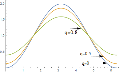
Figure 2: Time dependence of the throat radius $r(0,\eta)$ for $q=0,0.5,0.8$

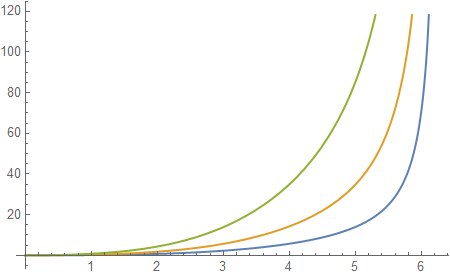
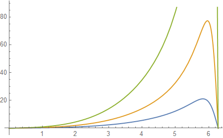
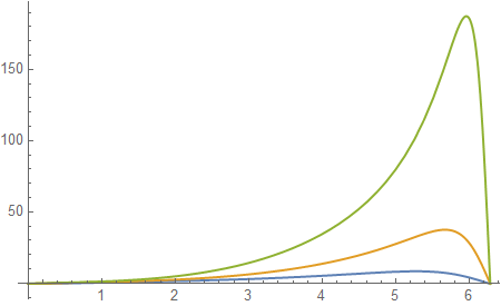
Figure 3: Time dependence of $r^{\prime}(x,\eta)$ for $q=0$ (left), $q=0.5$ (middle) and $q=0.9$ (right).

.

It is of interest that the dependence of the proper time $\tau$ on the time parameter $\eta$ is almost insensitive to a nonzero “charge” $q$, see Fig. 4.

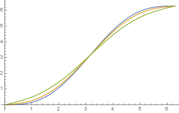
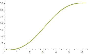
Figure 4: Proper time $\tau$ in terms of $\eta$ for $q=0,0.5,0.8$ on the throat $x=0$ (left, the plot is less steep for larger $q$) and $x=1$ (right, the plots almost merge).

As we already know, the equality $r^{\prime}=0$, if not on a throat, means that there is a singularity with infinite matter density, and to have finite $\rho>0$ we need $r^{\prime}>0$ at $x>0$ and $r^{\prime}<0$ at $x<0$. As follows from calculations and is illustrated in Fig. 3, we observe a good wormhole behavior of our solution at all $\eta\in(0,2\pi)$.

The density $\rho$ calculated according to (37) is also positive and well-behaved, as illustrated in Fig. 5. The density diverges as $\eta^{-6}$ at $\eta\to 0$, i.e., at the beginning of the evolution, and as $(2\pi-\eta)^{-3}$ at its end ($\eta\to 2\pi$) for dust ($q=0$) but is everywhere and always finite for $q\neq 0$, with qualitatively the same time dependence.

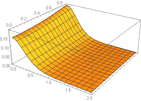
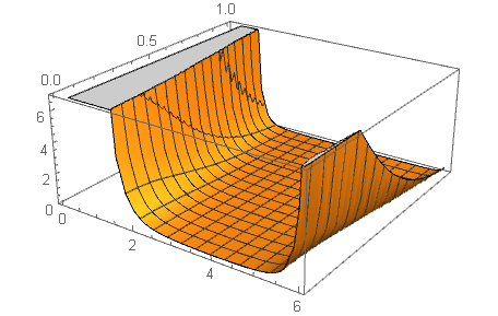
Figure 5: The quantity $\rho/(8\pi)$ as a function of $x$ and $q$ for $\eta=\pi$ (left) and as a function of $x$ and $\eta$ for $q=0$ (right).

Now, let us see how to inscribe such a wormhole into the cosmological model (46), (47). To match two q-LTB solutions with different choices of the arbitrary functions $F(R)$ and $h(R)$ at some value $R=R^{*}$, one should first of all identify the junction hypersurface as seen “from the left” and “from the right,” to be treated as the same surface in unified space-time, hence, in the metric (29) the coefficients $g_{\tau\tau}\equiv 1$ and $g_{\theta\theta}=r^{2}$ must coincide. For $g_{\tau\tau}$ it is trivial, while the requirement to the jump $[r^{2}]=0$ is meaningful. Next, to avoid the emergence of a thin shell of matter on the junction surface, its second quadratic form should also have no jump [30, 31]. For the metric (29), this requirement reduces to $[{\rm\,e}^{-\lambda}r^{\prime}]=0$, while a similar requirement to $g_{\tau\tau}$ is again trivial. With Eqs. (34) and (3.3), the above requirements take the form

$$[r]=0,\quad\ [{\rm\,e}^{-\lambda}r^{\prime}]=0\ \ \ \Rightarrow\ \ \ [h]=0,\quad[F]=0.$$ (55)

In other words, to match two particular solutions, we must simply identify the values of $F(R)$ and $h(R)$ on the junction surface. The charge $q$ should certainly be the same in both solutions to provide continuity of the electromagnetic field. It is of utmost importance that due to (3.3) these matching conditions hold at all times as long as both solutions remain regular. There is no need to adjust the radial coordinate choice in the two solutions since both $r$ and ${\rm\,e}^{-\lambda}r^{\prime}$ are insensitive to this choice, and consequently the same is true for $h(R)$ and $F(R)$ which behave as scalars under transformations of $R$.

Let us apply the conditions (55) to the solutions (46), (47) and (53), (54), in which we must put $q=0$. If the junction surface is specified by $\chi=\chi^{*}$ and $x=x^{*}$, we obtain

$$x^{*}=\cot\chi^{*},\qquad b=a_{0}\sin^{5}\chi^{*}.$$ (56)

This ensures matching at $x^{*}>0$. With the even functions (53), the same matching is implemented at $x^{*}<0$, and the whole configuration consists of two closed evolving Friedmann universes connected through a wormhole, and one can imagine something like a dumbbell (replacing 3D spherical spaces with 2D spherical surfaces).

Some numerical estimates are in order. Assuming $a_{0}\sim 10^{28}$ cm, approximately the size of the visible part of our Universe, let us require that the throat radius $r_{\rm th}\sim b$ should be much larger that the Planck length, $b\gg l_{\rm pl}\sim 10^{-33}$ cm. Then from (56) it is easy to obtain

$$\sin\chi^{*}\gg 10^{-12},\qquad x^{*}\ll 10^{12},$$ (57)

so that $r^{*}=r(x^{*})\gg 10^{16}$ cm $\sim 0.01$ light year. Thus the wormhole region must be large enough on the astronomical scale in order to provide a reasonable size of the throat. Assuming $r^{*}\sim 100$ light years, the size of a small stellar cluster, we obtain $\chi^{*}\sim 10^{-8}$ and $r_{\rm th}\sim 10^{20}l_{\rm pl}$, approximately the nuclear size of the throat. Assuming a galactic size of the wormhole region, $r^{*}\sim 30\ {\rm kpc}\sim 10^{23}$ cm, we have $\chi\sim 10^{-5}$ and consequently $r^{*}\sim 10^{3}$ cm, a macroscopic size of the throat.

The density obeys Eq. (37), which for our model (53) and $q=0$ gives

$$\rho=\frac{1}{2\pi Gb^{2}}\,\frac{1}{(1+x^{2})^{5}(1-\cos\eta)(2N_{2}-N_{1})}$$ (58)

where $2N_{2}-N_{1}$ is, for $\Delta=1$, a function of $\eta$, positive in the range $\eta\in(0,2\pi)$. The time-dependent part of (58) may be approximated by $1/10$, which is true for a larger part of the time range, and then we obtain, by order of magnitude,

$$\rho\sim\frac{10^{-30}}{(1+x^{2})^{5}\sin^{10}\chi^{*}}\ \rm g/cm^{3}.$$ (59)

For the throat $x=0$ this expression gives about $10^{50}\ \rm g/cm^{3}$ if $\chi^{*}=10^{-8}$ and about $10^{20}\ \rm g/cm^{3}$ if $\chi^{*}=10^{-5}$, a value still substantially exceeding the nuclear density. On the other hand, since $x^{*}\sim 1/\chi^{*}$, for the density at the junction surface $x=x^{*}$ we obtain a universal value of $\sim 10^{-30}\ \rm g/cm^{3}$, close to the mean cosmological density, independently of the $\chi^{*}$ value.

Such estimates will certainly change, though probably not too drastically, if we choose $F(R)$ and $h(R)$ other than in (53).

The same procedure applied to solutions with $q\neq 0$ would describe a wormhole joining two Friedmann universes deformed by the magnetic field, but their discussion is beyond the scope of this paper.

4 Wormholes leading to extra dimensions

The studies of multidimensional wormholes are as diverse as are multidimensional extensions of GR. Therefore, let us here, without trying to review this vast area of research, which can be a subject of a much larger project, simply refer to a number of relevant papers [80, 81, 82, 83, 84, 85, 86, 87, 88, 89], where further references can be found. In this section we consider a case of interest where the size of compact extra dimensions is small enough at one entrance to a wormhole to make them invisible and is much larger at the other entrance [17, 18]. Such solutions to the field equations thus describe a transition from an effectively 4D geometry to a multidimensional space-time.

4.1 Field equations

Consider 6-dimensional GR with a minimally coupled scalar field $\phi$ with a potential $V(\phi)$ as the only source of gravity. The Lagrangian is

$$L=R_{6}+2\varepsilon_{\phi}g^{AB}\partial_{A}\phi\partial_{B}\phi-2V(\phi),$$ (60)

where $R_{6}$ is the 6D Ricci scalar, $\varepsilon_{\phi}$ is $+1$ for a canonical scalar field and $-1$ for a phantom one, and $A,B,\ldots=\overline{0,5}$. The equations of motion include the scalar field equation $2\varepsilon_{\phi}\Box_{6}\phi+dV/d\phi=0$ ($\Box_{6}=\nabla^{A}\nabla_{A}$ is the 6D d’Alembertian) and the Einstein equations which may be written in the form

$${}R^{A}_{B}=-{\tilde{T}}^{A}_{B}\equiv-T^{A}_{B}-\tfrac{1}{4}\delta^{A}_{B}T^{C}_{C}=-2\varepsilon_{\phi}\partial^{A}\phi\partial_{B}\phi+{\tfrac{1}{2}}V(\phi)\delta^{A}_{B},$$ (61)

$R^{A}_{B}$ being the 6D Ricci tensor and $T^{A}_{B}$ the scalar field SET.

Let the 6D space-time be a direct product of three 2D subspaces, ${\mathbb{M}}={\mathbb{M}}_{0}\times{\mathbb{M}}_{1}\times{\mathbb{M}}_{2}$, where ${\mathbb{M}}_{0}$ is 2D Lorentzian space-time parametrized by the coordinates $x^{0}=t$ and $x^{1}=x$, while ${\mathbb{M}}_{1}$ and ${\mathbb{M}}_{2}$ are compact spaces of nonnegative constant curvature, i.e., each of them is either a sphere or a torus. The 6D metric is assumed in the form:

$$ds^{2}=A(x)dt^{2}-\frac{dx^{2}}{A(x)}-R(x)d\Omega_{1}^{2}-P(x)d\Omega_{2}^{2},$$ (62)

where $A(x),\ R=r^{2}(x),\ P=p^{2}(x)$ depend on the “radial” coordinate $x$, satisfying the condition $g_{tt}g_{xx}=-1$ (the “quasiglobal gauge” [5]), while $d\Omega_{1}^{2}$ and $d\Omega_{2}^{2}$ are $x$-independent metrics on the manifolds ${\mathbb{M}}_{1}$ and ${\mathbb{M}}_{2}$ of unit size. It is also assumed $\phi=\phi(x)$.

We do not specify which of the subspaces ${\mathbb{M}}_{1,2}$ belongs to our “external” 4D space-time and which is “extra.” Thus, if ${\mathbb{M}}_{1}$ is large and spherical while ${\mathbb{M}}_{2}$ is small and toroidal, we have a static, spherically symmetric 4D space-time with a toroidal extra space; if $M_{1}$ is small and spherical and ${\mathbb{M}}_{2}$ is large and toroidal, then we are dealing with toroidally symmetric 4D space-time and a spherical extra space, and so on.

The scalar field equation can be derived from (61), and among the latter there are four independent ones, which may be written in the form

$$R^{t}_{t}=-{\tilde{T}}^{t}_{t}\ \ \Rightarrow\ \ -(PR)^{-1}(A^{\prime}PR)^{\prime}=V(\phi),$$ (63)

$$R^{t}_{t}-R^{x}_{x}=-{\tilde{T}}^{t}_{t}+{\tilde{T}}^{x}_{x}\ \ \Rightarrow\ \ \frac{r^{\prime\prime}}{r}+\frac{p^{\prime\prime}}{p}=-\varepsilon_{\phi}\phi^{\prime}{}^{2},$$ (64)

$$R^{t}_{t}-R^{\underline{a}}_{a}=0\ \ \Rightarrow\ \ [P(AR^{\prime}-A^{\prime}R)]^{\prime}=2\varepsilon_{1}P,$$ (65)

$${}R^{t}_{t}-R^{\underline{m}}_{m}=0\ \ \Rightarrow\ \ [R(AP^{\prime}-A^{\prime}P)]^{\prime}=2\varepsilon_{2}R,$$ (66)

where the prime denotes $d/dx$, the index $a=2,3$ (belonging to ${\mathbb{M}}_{1}$), while $m=4,5$ (belonging to ${\mathbb{M}}_{2}$), and there is no summing over an underlined index; furthermore, $\varepsilon_{1}=1$ if ${\mathbb{M}}_{1}$ is a sphere and $\varepsilon_{1}=0$ if it is a torus, and similarly for $\varepsilon_{2}$ and ${\mathbb{M}}_{2}$.

Equations (65) and (66) can be considered separately as two equations for the three metric functions $A(x),P(x),R(x)$, so that there is arbitrariness in one function. Further, if we know the metric functions, we can use the other two equations, (63) and (64), to find the scalar field $\phi$ and the potential $V$.

As follows from Eq. (64), if we assume that $r>0$ and $p>0$ in the whole range $x\in{\mathbb{R}}$, this is only compatible with $\varepsilon_{\phi}=-1$, a phantom scalar, otherwise at least one of these radii will turn to zero at some finite $x$.

4.2 Possible asymptotic behavior of the metric

The following types of geometry are possible with the metric (62):

(i)

SS (double spherical) space-times if $\varepsilon_{1}=\varepsilon_{2}=1$.

(ii)

ST (spherical-toroidal) space-times if $\varepsilon_{1}=1,\ \varepsilon_{2}=0$ or vice versa.

(iii)

TT (double toroidal) space-times if $\varepsilon_{1}=\varepsilon_{2}=0$.

For any of these types, we are interested in configurations where $x\in{\mathbb{R}}$ and where one of the subspaces ${\mathbb{M}}_{1}$ or ${\mathbb{M}}_{2}$ is large on both ends $x\to\pm\infty$ while the size of the other is radically different. In particular, a 4D flat asymptotic region times small extra dimensions as $x\to-\infty$ and something different on the other end.

Some restrictions can be obtained from the analysis of Eqs. (65) and (66), without addressing the scalar field properties. Consider, for example, a 4D asymptotically flat space-time with everywhere finite extra dimensions in SS geometry. It means that

$$A(x)\to{\rm finite},\quad\ R(x)\sim x^{2},\quad\ P(x)\to{\rm finite}\quad{\rm as}\ \ x\to\infty.$$ (67)

Let us use these conditions in Eqs. (65) and (66). From (67) it follows that $R^{\prime}\sim x$, $A^{\prime}\sim x^{-3}$ or even smaller (since for a finite limit of $A$ it should be $A=A_{-}+A_{-2}/x^{2}+\ldots$), and the l.h.s. of (65) tends, in general, to a nonzero constant, which conforms to the assumed limit of $P$ on the r.h.s.. However, the expression in square brackets in Eq. (66) tends to a constant, its derivative thus vanishes, whereas the r.h.s. is $2R\sim x^{2}$. We have to conclude that the conditions (67) contradict the field equations.

The same reasoning applies to $x\to-\infty$ and/or exchanged $R(x)$ and $P(x)$. Other opportunities can be tested in the same manner. An analysis shows [18] that SS space-times cannot possess a flat Minkowski asymptotic region times a sphere of finite size, while a de Sitter behaviour times a finite sphere can take place. In ST geometry, we can obtain effectively 6D asymptotics (that is, $R$ and $P$ equally large), as well as an asymptotically flat spherically symmetric 4D space-time times constant extra dimensions. In general, one can obtain similar or different asymptotic behaviors at the two ends, $x\to\pm\infty$. We will present two examples of such solutions to Eqs. (63)–(66) with a 4D geometry with small extra dimensions at one end and an effectively 6D geometry at the other.

4.3 Example 1: ST geometry, wormholes with a massless scalar

An asymptotically flat spherically symmetric geometry with small extra dimensions at one end and the same with much larger extra dimensions at the other can be found among known solutions for a massless scalar field ($V=0$) [90, 91]. The solution of interest has the form [17]

$${}ds^{2}=dt^{2}-{\rm\,e}^{-4nu}\big{[}dz^{2}+(z^{2}+k^{2})d\Omega_{1}^{2}\big{]}-{\rm\,e}^{2nu}d\Omega_{2}^{2},$$

$${}\phi=Cu\equiv(C/k)\cot^{-1}(-z/k),$$ (68)

where $z\in{\mathbb{R}}$, $n>0,\ C,\ k>0$ are integration constants connected by the relation $2C^{2}=k^{2}+3n^{2}$. In the 4D subspace ${\mathbb{M}}_{0}\times{\mathbb{M}}_{1}$ it represents a spherically symmetric, twice asymptotically flat wormhole, while the extra subspace ${\mathbb{M}}_{2}$ is toroidal, with its coordinates $x^{4},x^{5}$ ranging from zero to some fixed length $a$. Thus at $z=-\infty$ (hence $u=0$) the size of extra dimensions is equal to $a$, while at the other end, $u=\pi/k$, corresponding to $z=+\infty$, we have the size $a_{+}={\rm\,e}^{n\pi/k}a$. In the trivial case $n=0$ the solution reduces to the Ellis 4D wormhole [92, 93] times an extra 2D toroidal space of constant size.

Let us suppose that the size $a$ of extra dimensions at the left end, $z=-\infty$, is sufficiently small to be invisible for the existing experimental means, say, $a=10^{-17}$ cm. The size $a_{+}$ corresponding to $z\to\infty$ depends on the ratio $n/k$ and can be arbitrarily large. Thus, we obtain $p_{+}\sim 1$ m if we take $n/k\approx 14$. To get a size of stellar order, $p_{+}\sim 10^{6}\ {\rm km}=10^{11}$ cm, we should assume $n/k\approx 20.5$.

The wormhole throat is found at a minimum of the 4D radius $r$ ($g_{22}={\rm\,e}^{-4nu}(z^{2}+k^{2})$), which occurs at $z=2n$ and is given by

$$r_{\min}=\sqrt{k^{2}+4n^{2}}\exp{\Big{(}\frac{2n}{k}\cot^{-1}\frac{2n}{k}\Big{)}}.$$ (69)

This radius can be made sufficiently large by properly choosing the parameters $k$ and $n$. Thus, if $n/k\gg 1$ (as required for obtaining large $a_{+}$), we have $r_{\min}\approx 2n{\rm\,e}\approx 5.4n$, and the lengths $n$ and $k$ should be very large as compared to $a$. For example, to have the throat size $r_{\min}=10$ m, large enough to transport macroscopic bodies, we should take $n\sim 2\ {\rm m}=2\times 10^{19}a$.

4.4 Example 2: ST geometry, asymptotically AdS wormholes

Solutions to Einstein-scalar equations with nonzero potentials $V(\phi)$ can be found, in most cases, only numerically. For our system (63)–(66), there is an exception: assuming $\varepsilon_{2}=0$, integrating Eq. (66) and putting the emerging integration constant equal to zero, we obtain $P=cA$, $c={\rm const}$, and Eq. (65) takes the form $A^{3}(R/A)^{\prime}]^{\prime}=2A$, that is, one equation for two functions $A(x)$ and $R(x)$. It may be rewritten as

$$\Big{(}\frac{R}{A}\Big{)}^{\prime}=\frac{2}{A^{3}}\int A(x)dx.$$ (70)

and is thus solved by quadratures if the function $A(x)$ is specified. Let us try to obtain a configuration where the 4D subspace is asymptotically flat on the left end and tends to AdS behavior on the right. We thus suppose $A\to 1$ as $x\to-\infty$ and $A\sim x^{2}$ as $x\to+\infty$. It is rather hard to invent $A(x)$ with such asymptotic properties that would yield more or less simple analytic expressions for other quantities. Therefore, we have obtained a desirable example by choosing a piecewise smooth function $A(x)$ [17]:

$$A(x)=1,\ \ x\leq 0;\qquad A(x)=1+3x^{2}/a^{2},\ \ x\geq 0\qquad(a={\rm const}>0).$$ (71)

The resulting metric is $\rm C^{1}$ smooth, but there are jumps in the functions $\phi^{\prime}(x)$ and $V(x)$ (Fig. 6). As mentioned above, the relation $P=cA$ holds at all $x$, while $R(x)$ is given by

$$R(x)=x^{2}+b^{2}\ \ (x\leq 0),\qquad R(x)=\Big{(}1+\frac{3x^{2}}{a^{2}}\Big{)}\biggl{[}b^{2}+\frac{x^{2}(1+2x^{2}/a^{2})}{(1+3x^{2}/a^{2})^{2}}\biggr{]}\ \ (x\geq 0),$$ (72)

with $b={\rm const}>0$ (so that $x=0$ is a throat of radius $b$). At $x<0$ the scalar field is massless, $V(x)\equiv 0$, and $\phi(x)=\arctan(x/b)$, while at $x>0$ the corresponding expressions are rather bulky.

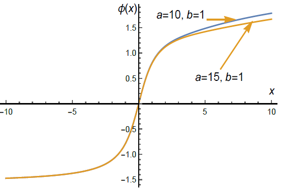
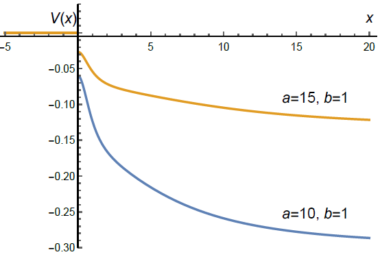
Figure 6: The scalar field $\phi(x)$ (left) and the potential $V(x)$ (right) in example 2

We obtain a configuration which is asymptotically flat times constant (arbitrarily small) extra dimensions on one side of the wormhole and behaves as a 6D AdS space on the other side, with the potential $V$ tending to a negative constant value, becoming there an effective cosmological constant.

Let us note that it is easy to remove the jumps in $V(x)$ and $\phi^{\prime}(x)$ at $x=0$ by adding arbitrarily small quantities to $A(x)$ making it smoother than $\rm C^{1}$.

5 Conclusion

We have considered three different kinds of wormholes in GR, showing some possible nonstandard features of these hypothetic objects.

The existence of stationary cylindrical wormholes respecting the WEC not only shows a way to circumvent topological censorship but also illustrates the exotic properties of vortex gravitational fields due to rotation, see Eq. (2.4). Similar solutions in the cosmological context were obtained and discussed in [94]. The results of [48, 49], where spherically symmetric wormholes were obtained with spinor sources of gravity, probably show that the spin of matter can also manifest exotic properties, and this issue deserves a further study. One can notice that topology alone, without rotation, cannot lead to viable phantom-free wormhole solutions, as follows, in particular, from the properties of static cylindrical wormholes [26] and the recently obtained static toroidal wormholes [95].

Cosmological wormholes can probably be relevant in the early Universe, and the presently reported results show that they could naturally exist not only at the inflationary stage but also at the matter-dominated one. It supports the idea that wormholes with de Sitter asymptotic regions that existed at the inflationary stage might somehow survive at the radiation-dominated and later stages and still exist in the present Universe, as is discussed by a number of researchers, e.g., in [96, 97, 66, 70, 98] and others.

In 6D GR with a minimally coupled phantom scalar as a source of gravity, we have constructed examples of space-times which are effectively 4D in a certain part of the whole space-time and effectively 6D on the far end. The existence of such “bubbles” or their analogues with a different number of extra dimensions, surrounded by domain walls, in our Universe cannot be a priori excluded, as shown, in particular, in [99], and their possible observational consequences can be a subject of further studies. One of such consequences can be black hole formation due to domain wall shrinking, which, if these “bubbles” were numerous enough in the early Universe, could result in a wealth of primordial black holes substantially contributing to the Dark Matter density [99]. As follows from our discussion, the anomalous domains can communicate with those of conventional 4D physics not only by photons or gravitational waves crossing the domain walls, but also through wormholes.

Acknowledgments.

I thank Milena Skvortsova, Sergei Bolokhov, Sergey Sushkov and Pavel Kashargin for collaboration and helpful discussions. This publication was supported by the RUDN University Strategic Academic Leadership Program. It was also funded by the Ministry of Science and Higher Education of the Russian Federation, Project “Fundamental properties of elementary particles and cosmology” N 0723-2020-0041, and by RFBR Project 19-02-00346.

References

- [1] L. Flamm, Beiträge zur Einsteinschen Gravitationstheorie, Phys. Z. 17, 448 (1916).
- [2] A. Einstein and N. Rosen, The particle problem in the general theory of relativity, Phys. Rev. 48, 73-77 (1935).
- [3] M. Visser, Lorentzian Wormholes: From Einstein to Hawking (Springer-Verlag, Berlin, 1997).
- [4] F.S.N. Lobo, Exotic solutions in general relativity: Traversable wormholes and “warp drive” spacetimes. In: Classical and Quantum Gravity Research (Nova Science Publishers, NY, 2008), p. 1–78.
- [5] K.A. Bronnikov and S.G. Rubin, Black Holes, Cosmology and Extra Dimensions (2nd edition, World Scientific, Singapore, 2021).
- [6] J.L. Friedman, K. Schleich and D.M. Witt, Topological Censorship, Phys. Rev. Lett. 71, 1486 (1993); Erratum: Phys. Rev. Lett. 75, 1872(E) (1995).
- [7] G.J. Galloway, On the topology of the domain of outer communication, Class. Quantum Grav. 12, L99 (1995).
- [8] K.A. Bronnikov and V.G. Krechet, Potentially observable cylindrical wormholes without exotic matter in GR, Phys. Rev. D 99, 084051 (2019); arXiv: 1807.03641.
- [9] S.V. Bolokhov, K.A. Bronnikov, and M.V. Skvortsova, Cylindrical wormholes: A search for viable phantom-free models in GR, Int. J. Mod. Phys. D 28, 1941008 (2019); arXiv: 1903.09862.
- [10] K.A. Bronnikov, V.G. Krechet and V.B. Oshurko, Rotating Melvin-like universes and wormholes in general relativity, Symmetry 2020, 12, 1306 (2020); arXiv: 2007.01145.
- [11] K.A. Bronnikov, K.A. Baleevskikh and M.V. Skvortsova, Wormholes with fluid sources: A no-go theorem and new examples, Phys. Rev. D 96, 124039 (2017); arXiv: 1708.02324.
- [12] P. Kashargin and S. Sushkov, Collapsing wormholes sustained by dustlike matter, Universe 6 (10), 186 (2020).
- [13] K.A. Bronnikov, P. Kashargin and S.V. Sushkov, Magnetized dusty black holes and wormholes, in preparation.
- [14] G. Lemaître, L’Univers en expansion, Ann. Soc. Sci. Brussels A 53, 51 (1933); reprinted: Gen. Rel. Grav. 29, 641 (1997).
- [15] R.C. Tolman, Effect of inhomogeneity on cosmological models, Proc. Nat. Acad. Sci. USA 20, 169 (1934); reprinted: Gen. Rel. Grav. 29, 931 (1997).
- [16] H. Bondi, Spherically symmetrical models in general relativity, Mon. Not. R. Astron. Soc. 107, 410 (1947). reprinted: Gen. Rel. Grav. 31, 1783 (1999).
- [17] K.A. Bronnikov and M.V. Skvortsova, Wormholes leading to extra dimensions. Grav. Cosmol. 22, 316 (2016).
- [18] K.A. Bronnikov, P.A. Korolyov, A, Makhmudov and M.V. Skvortsova, Wormholes and black universes communicated with extra dimensions, J. Phys. Conf. Series 798, 012091 (2017).
- [19] M. Morris, K. S. Thorne, and U. Yurtsever, Wormholes, time machines, and the Weak Energy Condition, Phys. Rev. Lett. 61, 1446 (1988).
- [20] D. Hochberg and M. Visser, Geometric structure of the generic static traversable wormhole throat, Phys. Rev. D 56, 4745 (1997).
- [21] D. Zipoy, Topology of some spheroidal metrics. J. Math. Phys. 7, 1137-1143 (1966).
- [22] K.A. Bronnikov and J.C. Fabris, Weyl spacetimes and wormholes in D-dimensional Einstein and dilaton gravity, Class. Quantum Grav. 14, 831-842 (1997).
- [23] Gérard Clément, Spinning ring wormholes: a classical model for elementary particles? arXiv: gr-qc/9810075.
- [24] A. Burinskii, Stringlike structures in the real and complex Kerr-Schild geometry, J. Phys. Conf. Ser. 532, 012004 (2014); arXiv: 1410.2462.
- [25] K.A. Bronnikov, Static, cylindrically symmetric Einstein-Maxwell fields, in Problems in gravitation theory and particle theory (PGTPT) (Ed. K.P. Staniukovich, 10th issue, p. 37–50, Atomizdat, Moscow, 1979, in Russian).
- [26] K.A. Bronnikov and José P.S. Lemos, Cylindrical wormholes, Phys. Rev. D 79, 104019 (2009).
- [27] K.A. Bronnikov, Nilton Santos and Anzhong Wang, Cylindrical systems in general relativity (review). Class. Quantum Grav. 37, 113002 (2020); arXiv: 1901.06561.
- [28] K.A. Bronnikov, V.G. Krechet, and José P.S. Lemos, Rotating cylindrical wormholes. Phys. Rev. D 87, 084060 (2013); arXiv: 1303.2993.
- [29] V.G. Krechet and D.V. Sadovnikov, Spin-spin interaction in general relativity and induced geometries with nontrivial topology, Grav. Cosmol. 15, 337 (2009).
- [30] G. Darmois, Les équations de la gravitation einsteinienne. In: Mémorial des Sciences Mathematiques, vol. 25 (Gauthier-Villars, Paris, 1927).
- [31] W. Israel, Singular hypersurfaces and thin shells in general relativity. Nuovo Cim. B 48, 463 (1967).
- [32] K.A. Bronnikov, Rotating cylindrical wormholes: A no-go theorem. J. Phys. Conf. Series 675, 012028 (2016); arXiv: 1509.06924.
- [33] H. Stephani, D. Kramer, M.A.H. MacCallum, C. Hoenselaers, E. Herlt, Exact Solutions of Einstein’s Field Equations, Cambridge Monographs on Mathematical Physics (Cambridge University Press, 2009).
- [34] J. Safko and L. Witten, Some properties of cylindrically symmetric gravitational field, Phys. Rev. D 5, 293–300 (1972).
- [35] A.B. Evans, Static fluid cylinders in general relativity, J. Phys. A: Math. Gen. 10, 1303–1311 (1977).
- [36] K.A. Bronnikov, Static fluid cylinders and plane layers in general relativity, J. Phys. A: Math. Gen. 12, 201–207 (1979).
- [37] K.A. Bronnikov, V. Abdel-Sattar, E.N. Chudaeva and G.N. Shikin, Static, cylindrically symmetric perfect fluid configurations, Vestnik RUDN 1, 85–95 (2009).
- [38] K.A. Bronnikov, Gravitational and sound waves in stiff matter, J. Phys. A: Math. Gen. 13, 3455–3463 (1980).
- [39] N.O. Santos and R.P. Mondaini, Rigidly rotating relativistic generalized dust cylinder. Nuovo Cim. B 72, 13 (1982).
- [40] D. Sklavenites, Stationary perfect fluid cylinders, Class. Quantum Gravity 16, 2753 (1999).
- [41] B.V. Ivanov, On rigidly rotating perfect fluid cylinders, Class. Quantum Gravity 19, 3851 (2002).
- [42] F. Debbasch, L. Herrera, P.R.C.T. Pereira, and N.O. Santos, Stationary cylindrical anisotropic fluid, Gen. Rel. Grav. 38, 1825 (2006); gr-qc/0609068.
- [43] S.V. Bolokhov, K.A. Bronnikov, and M.V. Skvortsova. Rotating cylinders with anisotropic fluids in general relativity. Grav. Cosmol. 25 122–130 (2019); arXiv: 1904.06727.
- [44] S.D. Odintsov, V.K. Oikonomou, The early-time cosmology with stiff era from modified gravity, arXiv: 1711.04571
- [45] G. Brando, J.C. Fabris, F.T. Falciano, O. Galkina, Stiff matter solution in Brans-Dicke theory and the general relativity limit, arXiv: 1810.07860
- [46] V.A. Berezin, V.A. Kuzmin, and I.I. Tkachev, Dynamics of bubbles in general relativity, Phys. Rev. D 36, 2919 (1987).
- [47] A. Vilenkin, Gravitational Field of Vacuum Domain Walls and Strings, Phys. Rev. D 23, 852 (1981).
- [48] Jose Luis Blázquez-Salcedo, Christian Knoll, and Eugen Radu, Traversable wormholes in Einstein-Dirac-Maxwell theory, Phys. Rev. Lett. 126, 101102 (2021); arXiv: 2010.07317.
- [49] R. A. Konoplya and A. Zhidenko, Traversable wormholes in general relativity without exotic matter, arXiv: 2106.05034.
- [50] Kirill Bronnikov, Sergey Bolokhov, Serguey Krasnikov, and Milena Skvortsova, Comment on “Traversable wormholes in Einstein-Dirac-Maxwell theory,” arXiv: 2104.10933.
- [51] Mariam Bouhmadi-López, Che-Yu Chen, Xiao Yan Chew, Yen Chin Ong and Dong-han Yeom, Traversable wormhole in Einstein 3-form theory with self-interacting potential. arXiv: 2108.07302.
- [52] D. Hochberg and M. Visser, Dynamic wormholes, antitrapped surfaces, and energy conditions, Phys. Rev. D 58, 044021 (1998).
- [53] S. A. Hayward, Dynamic wormholes, Int. J. Mod. Phys. D 8, 373 (1999); gr-qc/9805019.
- [54] Y. Tomikawa, K. Izumi and T. Shiromizu, New definition of a wormhole throat, Phys. Rev. D 91, 104008 (2015).
- [55] E. Bittencourt, R. Klippert, and G.B. Santos, Dynamical wormhole definitions confronted, Class.Quantum Grav. 35, 55009 (2018); 1707.01078.
- [56] Hideki Maeda, Tomohiro Harada and B.J. Carr, Cosmological wormholes, Phys. Rev. D 79, 044034 (2009); arXiv: 0901.1153.
- [57] J.P.S. Lemos, F.S.N. Lobo and S.Q. de Oliveira, Morris-Thorne wormholes with a cosmological constant, Phys. Rev. D 68, 064004 (2003); gr-qc/0302049.
- [58] Mauricio Cataldo and Sergio del Campo, Two-fluid evolving Lorentzian wormholes, Phys. Rev. D 85,104010 (2012); arXiv: 1204.0753.
- [59] K.A. Bronnikov and J.C. Fabris, Regular phantom black holes, Phys. Rev. Lett. 96, 251101 (2006); gr-qc/0511109.
- [60] K.A. Bronnikov, H. Dehnen and V.N. Melnikov, Regular black holes and black universes, Gen. Rel. Grav. 39, 973 (2007); gr-qc/0611022.
- [61] S.V. Bolokhov, K.A. Bronnikov, and M.V. Skvortsova, Magnetic black universes and wormholes with a phantom scalar, Class. Quantum Grav. 29, 245006 (2012); arXiv: 1208.4619.
- [62] K.A. Bronnikov, Scalar fields as sources for wormholes and regular black holes, Particles 2018, 1, 56–81 (2018); arXiv: 1802.00098.
- [63] Sayan Kar, Evolving wormholes and the weak energy condition, Phys. Rev. D 49, 862 (1994).
- [64] Sung-Won Kim, Cosmological model with a traversable wormhole, Phys. Rev. D 53, 6889 (1996).
- [65] Luis A. Anchordoqui, Diego F. Torres, Marta L. Trobo, and Santiago E. Perez Bergliaffa, Evolving wormhole geometries, Phys. Rev. D 57, 829 (1998); gr-qc/9710026.
- [66] Sergey V. Sushkov and Yuan-Zhong Zhang, Scalar wormholes in cosmological setting and their instability, Phys. Rev. D 77, 024042 (2008); arXiv: 0712.1727.
- [67] Anna Mokeeva and Vladimir Popov, Nonsingular Chaplygin gas cosmologies in universes connected by a wormhole, Grav. Cosmol. 19, 57 (2013); arXiv: 1205.1542.
- [68] A.V.B. Arellano and F.S.N. Lobo, Evolving wormhole geometries within nonlinear electrodynamics, Class. Quantum Grav. 23, 5811 (2006); gr-qc/0608003.
- [69] K. A. Bronnikov, Nonlinear electrodynamics, regular black holes and wormholes, Int. J. Mod. Phys. D 27, 1841005 (2018); arXiv: 1711.00087.
- [70] I. Bochicchio and Valerio Faraoni, A Lemaître–Tolman–Bondi cosmological wormhole, Phys. Rev. D 82, 044040 (2010); arXiv: 1007.5427.
- [71] M.A. Markov and V.P. Frolov, Metrics of the closed Friedman world perturbed by electric charge (to the theory of electromagnetic *friedmons*), Teor. Mat. Fiz. 3, 3–17 (1970).
- [72] M. Bailyn, Oscillatory behavior of charge-matter fluids with , Phys. Rev. D 8, 1036 (1973)
- [73] P.A. Vickers, Charged dust spheres in general relativity, Ann. Inst. Henri Poincaré A 18, 137 (1973).
- [74] D.D. Ivanenko, V.G. Krechet, and V.G. Lapchinskii, The dynamics of charged dust in the general theory of relativity, Sov. Phys. J. 16, 1675–1679 (1973); https://doi.org/10.1007/BF00893659.
- [75] Yu.A. Khlestkov, Three types of solutions of the Einstein-Maxwell equations, J. Exp. Teor. Fis. 41 (2), 188 (1975).
- [76] I.S. Shikin, An investigation of a class of gravitational fields for a charged dustlike medium, J. Exp. Teor. Fis. 40 (2), 215 (1975).
- [77] L.D. Landau and E.M. Lifshitz, The Classical Theory of Fields (4th ed., Butterworth-Heinemann, 1987).
- [78] Alexander Shatskiy, I.D. Novikov and N.S. Kardashev, New analytic models of traversable wormholes, Phys. Usp. 51, 457–464 (2008); arXiv: 0810.0468.
- [79] Yu. A. Khlestkov and L. A. Sukhanova, Internal structure of wormholes — geometric images of charged particles in general relativity, Grav. Cosmol. 24, 360 (2018).
- [80] Gérard Clément, A class of wormhole solutions to higher-dimensional general relativity, Gen. Rel. Grav, 16, 131 (1984).
- [81] K.A. Bronnikov, Block-orthogonal brane systems, black holes and wormholes, Grav. Cosmol. 4, 49 (1998); hep-th/9710207.
- [82] V. Dzhunushaliev and H.-J. Schmidt, Wormholes and flux tubes in the 7D gravity on the principal bundle with SU(2) gauge group as the extra dimensions, Phys. Rev. D 62, 044035 (2000); gr-qc/9911080.
- [83] A. DeBenedictis and A. Das. Higher-dimensional wormhole geometries with compact dimensions, Nucl. Phys. B 653, 279 (2003); gr-qc/0207077.
- [84] K.A. Bronnikov and Sung-Won Kim. Possible wormholes in a brane world, Phys. Rev. D 67, 064027 (2003).
- [85] Francisco S.N. Lobo. General class of braneworld wormholes, Phys. Rev. D 75, 064027 (2007).
- [86] Vladimir Dzhunushaliev and Vladimir Folomeev, Kaluza-Klein wormholes with the compactified fifth dimension, Mod. Phys. Lett. A 29, 1450025 (2014).
- [87] Gustavo Dotti, Julio Oliva, and Ricardo Troncoso. Static wormhole solution for higher-dimensional gravity in vacuum, Phys. Rev. D 75, 024002 (2007).
- [88] Peter K. F. Kuhfittig, Traversable wormholes sustained by an extra spatial dimension, Phys. Rev. D 98, 064041 (2018); arXiv: 1809.01993.
- [89] Anshuman Baruah and Atri Deshamukhya, Traversable wormholes in higher-dimensional theories of gravity, J. Phys.: Conf. Ser. 1330, 012001 (2019); arXiv: 1904.04928.
- [90] K.A. Bronnikov. Spherically symmetric solutions in D-dimensional dilaton gravity, Grav. Cosmol. 1, 67 (1995); gr-qc/9505020.
- [91] K.A. Bronnikov, V.D. Ivashchuk and V.N. Melnikov, The Reissner-Nordström problem for intersecting electric and magnetic -branes, Grav. Cosmol. 3, 203 (1997); gr-qc/9710054.
- [92] K.A. Bronnikov, Scalar-tensor theory and scalar charge. Acta Phys. Polon. B 4, 251 (1973).
- [93] H. Ellis, Ether flow through a drainhole: a particle model in general relativity, J. Math. Phys. 14, 104 (1973).
- [94] Mustapha Azreg-Aïnou, Rotating cosmological cylindrical wormholes in GR and TEGR sourced by anisotropic fluids, Physics of the Dark Universe 32, 100802 (2021); arXiv: 2012.03431.
- [95] Vladimir Dzhunushaliev, Vladimir Folomeev, Burkhard Kleihaus and Jutta Kunz, Thin-shell toroidal wormhole, Phys. Rev. D 99, 044031 (2019); arXiv:1901.07545.
- [96] T. A. Roman, Inflating Lorentzian wormholes, Phys. Rev. D 47, 1370 (1993); gr-qc/9211012.
- [97] N.S. Kardashev, I.D. Novikov and A.A. Shatskiy, Astrophysics of wormholes, Int. J. Mod. Phys. D 16, 909 (2007); astro-ph/0610441.
- [98] A.A. Kirillov and E.P. Savelova, Cosmological wormholes, Int. J. Mod. Phys.D 25,1650075 (2016); arXiv: 1512.01450.
- [99] K.A. Bronnikov and S.G. Rubin, Local regions with expanding extra dimensions, arXiv: 2107.13893.