Separable convolutions for optimizing 3D Stereo Networks

Abstract

Deep learning based 3D stereo networks give superior performance compared to 2D networks and conventional stereo methods. However, this improvement in the performance comes at the cost of increased computational complexity, thus making these networks non-practical for the real-world applications. Specifically, these networks use 3D convolutions as a major work horse to refine and regress disparities. In this work first, we show that these 3D convolutions in stereo networks consume up to $94$% of overall network operations and act as a major bottleneck. Next, we propose a set of “plug-&-run” separable convolutions to reduce the number of parameters and operations. When integrated with the existing state of the art stereo networks, these convolutions lead up to $7\times$ reduction in number of operations and up to $3.5\times$ reduction in parameters without compromising their performance. In fact these convolutions lead to improvement in their performance in the majority of cases.

Index Terms—  Stereo Matching, Separable Convolutions, Disparity Estimation, Computational Efficiency, CNNs

1 Introduction

Estimating depth from an input stereo pair is an actively pursued goal in the computer vision domain. This typically involves two steps: (i) image rectification based on epipolar constraints and (ii) disparity estimation. A typical disparity estimation pipeline mainly consists of matching cost computation and cost aggregation steps [1]. In the matching cost step, features are computed from both images and matched to generate a potential set of matches. In the cost aggregation step, global [2, 3] or local neighbourhood [4, 1] constraints are applied to refine the potential matches and generate the disparity values.

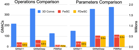
Fig. 1: Relative comparison between 3D convolutions, FwSCs, FDwSCs w.r.t. number of operations and parameters. Here $\times$ represents the reduction factor.

With the renaissance of deep learning, many new methods have been proposed to improve the overall density estimation pipeline. These methods target either a specific step [5, 6, 7] or work in end-to-end fashion [8, 9, 10] to improve the overall pipeline. End-to-end deep learning methods, in general, have two main stages. In the first stage, a backbone network is used to compute features from both the input images. In the second stage, features from both the images are merged to form a cost volume; this cost volume is then further processed via a sequence of convolutional layers to regress the final disparities. Broadly speaking, these end-to-end methods can be classified to 2D or 3D methods – depending on their methodology of merging features, types of layers and convolutions in the second stage – c.f. Sec. 2. Overall, 2D networks use 2D convolutions after merging features, whereas 3D methods use 3D convolutions over 4D cost volumes to regress and refine disparities.

Even though 3D methods give far superior performance compared to 2D methods, this performance improvement comes at the cost of extra computational budget. In fact, these 3D methods are orders of magnitude slower than 2D ones. A lot of efforts in the community have been recently targeted to make these methods computationally efficient [11, 12, 13]. Although majority of these methods target optimization of the cost-volume construction step, they still use the costly 3D convolutions for disparity regression. In this work, we aim to further reduce the overall computational footprint of the 3D methods by optimizing 3D convolutions.

For this, we first do a thorough empirical investigation of the state of the art 3D stereo methods [10, 9] to identify major contributing factors to the overall computational cost of these methods. As expected, our investigations conclude that 3D convolutions are by far the most costly operations in these methods. For instance, in GANetdeep, 3D convolutions consume around 94% of operations – c.f. Table 1. Next, we propose methods for optimizing 3D convolutions, i.e. how we can optimize 3D convolutions without sacrificing 3D stereo networks performance.

To this end, motivated by the recent performance of light-weight 3D networks for visual recognition [14, 15], we propose to replace costly 3D convolution operations in 3D stereo networks with their light-weight counterparts (i.e. separable 3D convolutions) to build efficient stereo networks. For this we design and explore three different versions of separable 3D convolutions: (i) Feature-wise Separable Convolutions (FwSCs); (ii) Disparity-wise Separable Convolutions (DwSCs); and their extremely separable version (iii) Feature-&-Disparity-wise Separable Convolutions (FDwSCs). We empirically evaluate these separable 3D convolution versions as “plug-&-run” replacement for existing 3D convolutions.

Overall, we make the following contributions: (i) we present an in-depth cost analysis of major building blocks of state of the art 3D stereo networks; (ii) we design and propose separable 3D convolutions for stereo networks; (iii) we empirically evaluate and show the “plug-&-run” characteristic of proposed convolutions for state of the art methods on standard datasets. Our results show that FwSCs and FDwSCs can be reliably used as a replacement for 3D convolutions in stereo networks without sacrificing their performance while reducing the number of operations (up to $7.2\times$) and number of parameters (up to $3.5\times$) – c.f. Fig. 1 & Table 3. To the best of our knowledge, this is the first work to explicitly optimize 3D convolutions involved in 3D stereo networks.

2 Related Work

Generally speaking, deep learning stereo methods can be broadly categorized into 2D or 3D learning methods [16] based on how they merge information across views and then process it. For instance, 2D methods merge features from the left and right images into a 3D cost volume and then apply 2D convolutions. DispNet-C [17], iResNet [18], MADNet [19], SegStereo [20], EdgeStereo [21] are some examples of 2D methods. On the other hand, 3D methods first generate a 4D cost volume by merging features from the left and right images (under stereo constraints) and use 3D convolutional layers to refine and regress dense disparities. GC-Net [8], PSMNet [9], GANet [10], AnyNet [11] and DeepPruner [13] are some examples of 3D methods. Overall 3D methods produce better results but at the expense of extra computational cost. Although recent methods propose to optimize the 3D cost volume construction step, they still use costly 3D convolutions for cost aggregations, refinement and disparity regression. For instance, [11] use hierarchical 3D cost volumes to reduce 4D volume construction cost while [12] introduce bottleneck matching modules to efficiently match features across disparities. In another work [13] employs patch-matching to sample a range of disparities during volume construction.

3 Methodology

Generally, an end-to-end 3D stereo pipeline consists of these modules: (i) Feature extraction: a 2D shared backbone-network to extract features from left and right images of a rectified stereo pair; (ii) Volume construction: a 4D cost volume constructed by merging left and right images features maps; and (iii) Cost aggregation & disparity regression: a 3D network to aggregate cost volume and then regress and refine disparities from aggregated cost volume.

Table 1: Detailed computational cost profiling of 3D stereo networks.

Model	Metric	Feature Network		Cost Aggregation and Disparity Regression		Total
		2D CNNs		3D CNNs
GANet11	# Params (M)	$\numprint{2.37}$	$\numprint{53.33}\%$	$\numprint{0.76}$	$\numprint{17.7}\%$	$\numprint{4.48}$
	# Ops (GMACs)	$\numprint{4.80}$	$\numprint{2.03}\%$	$\numprint{217.44}$	$\numprint{91.92}\%$	$\numprint{236.56}$
GANetdeep	# Params (M)	$\numprint{2.37}$	$\numprint{36.31}\%$	$\numprint{1.80}$	$\numprint{27.21}\%$	$\numprint{6.58}$
	# Ops (GMACs)	$\numprint{4.80}$	$\numprint{1.25}\%$	$\numprint{358.85}$	$\numprint{93.51}\%$	$\numprint{383.75}$
PSMNet	# Params (M)	$\numprint{3.34}$	$\numprint{63.52}\%$	$\numprint{1.89}$	$\numprint{36.5}\%$	$\numprint{5.22}$
	# Ops (GMACs)	$\numprint{58.19}$	$\numprint{31.40}\%$	$\numprint{127.12}$	$\numprint{68.6}\%$	$\numprint{185.31}$

3.1 Profiling 3D Stereo Networks

As the first step, we profile the overall computational requirements of the state of the art 3D stereo networks [10, 9]. Specifically, we record the number of parameters and operations involved in feature extraction and cost aggregation & disparity regression modules – c.f. Table 1. Here operations are reported as the number of MACs (Multiply-ACcumulate operations) where $1\mbox{MAC}=1$ multiplication + $1$ addition operations. We can observe from Table 1 that despite having fewer parameters than 2D networks, 3D networks consume more operations in all the networks and thus represent clear bottlenecks. For instance, in GANet11 [10] 3D CNN contains $0.8\times 10^{6}$ ($17\%$ relative to complete network) parameters compared to 2D feature extraction module’s $2.4\times 10^{6}$ parameters ($52.8\%$). However, it consumes $217$ GMACs operations ($91.9\%$ of overall operations) compared to $4.8$ GMACs ($2$ %) of the 2D network. Similar observations can be made about other networks.

Once we have built a detailed insight into the reasons behind these networks computational overhead, we set out to network design choices to reduce the computational overhead without compromising their performance.

3.2 Separable 3D Stereo Networks

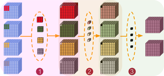
Fig. 2: Pictorial description of steps involved in the computation of FwSCs (left) and FDwSCs (right).

Model	#3D	Metric	3D	FwSCs		FDwSCs
	Convs		Convs		Reduction		Reduction
GANet11	$11$	# Params (M)	$\numprint{0.76}$	$\numprint{0.26}$	$2.9\times$	$\numprint{0.25}$	$3.0\times$
		# Ops (GMACs)	$\numprint{217.44}$	$\numprint{43.05}$	$5.1\times$	$\numprint{40.60}$	$5.4\times$
GANetdeep	$15$	# Params (M)	$\numprint{1.80}$	$\numprint{0.53}$	$3.4\times$	$\numprint{0.52}$	$3.5\times$
		# Ops (GMACs)	$\numprint{358.85}$	$\numprint{64.03}$	$5.6\times$	$\numprint{60.06}$	$6.0\times$
PSMNet	$22$	# Params (M)	$\numprint{1.89}$	$\numprint{0.58}$	$3.3\times$	$\numprint{0.57}$	$3.3\times$
		# Ops (GMACs)	$\numprint{127.12}$	$\numprint{19.06}$	$6.7\times$	$\numprint{17.70}$	$7.2\times$

Table 2: Comparison of 3D convolutions parameters and operations with separable 3D Convs.

Recently light-weight convolutional networks (like MobileNet, ShuffleNet, etc. [22, 23]) have been proposed to improve the computational efficiency of 2D visual recognition convolutional networks. These methods propose to use depth-wise separable variants of 2D convolutions to reduce the number of operations. However, in comparison to a 2D convolution kernel, a 3D convolution kernel works on a 4D volume and aggregates information across spatial, depth and channels dimensions, and thus there are different possible ways a 3D convolution can be made separable. For instance, a 3D kernel ($k\times k\times k$, e.g. $k=5$) working on an input 4D cost volume of size $h_{i}\times w_{i}\times d_{i}\times c_{i}$ (input height, width, depth (disparity), and channels) aggregates information from a window of size $k\times k\times k\times c_{i}$ in each of its applications. Furthermore, as a 3D convolutional layer contains many 3D kernels each producing a new feature map so overall there are $(h_{i}\times w_{i}\times d_{i}\times(k\times k\times k\times c_{i}))\times c_{o}$ operations performed in each layer – here $c_{o}$ is number of output channels (number of kernels) in a layer. From this, we can see that these 3D convolutions can be made separable across either $d_{i}$ or $c_{i}$ dimension or even simultaneously both across $d_{i}$ and $c_{i}$. We intend to reduce computational requirement by making 3D convolutions separable in one or more of the given dimensions.

3.2.1 Feature-wise Separable Convolutions (FwSCs):

As a first replacement for 3D convolutions in stereo networks, we propose to split the convolutions across the feature (or channel) dimension. FwSCs works in two steps: in the first step, the 4D cost volume of size $h_{i}\times w_{i}\times d_{i}\times c_{i}$ is split into $c_{i}$ cubes, and $c_{i}$ kernels of size $k\times k\times k$ are applied to generate $c_{i}$ output cubes – c.f. Fig. 2 (left).

In the second step, $c_{o}$ point-wise kernels of size $1\times 1\times 1\times c_{i}$ are applied to aggregate information across the $c_{i}$ cubes. These steps lead to a significant reduction in the number of operations, as total the number of operations reduces to $(h_{i}\times w_{i}\times d_{i}\times k\times k\times k)\times c_{i}+(h_{i}\times w_{i}\times d_{i}\times 1\times 1\times 1\times c_{i})\times c_{o}$ compared to 3D convolutions. When applied in the state of the art stereo networks, FwSCs lead up to $6.7\times$ reduction in GMACs (see Table 2) with better performance than 3D convolutions in the majority of cases (Sec. 4).

3.2.2 Disparity-wise Separable Convolutions (DwSCs):

DwSCs are identical to FwSCs, except the separable operation is performed in the disparity dimension. Precisely, in the first step the 4D cost volume of size $h_{i}\times w_{i}\times d_{i}\times c_{i}$ is split into $d_{i}$ cubes (after permuting $h_{i}\times w_{i}\times d_{i}\times c_{i}$ to $h_{i}\times w_{i}\times c_{i}\times d_{i}$) and $d_{i}$ kernels of size $k\times k\times k$ are applied to produce $d_{i}$ output cubes.

In the second step, $c_{o}$ kernels of size $1\times 1\times 1\times d_{i}$ are applied to aggregate information across the $d_{i}$ cubes. Finally, the output volume is permuted back. Although DwSCs lead to a reduction in the number of operations, the overall reduction is not as significant as in FwSCs, because usually in stereo networks size of disparity dimension is greater than the size of feature dimension. For instance, in GANetdeep the size of disparity dimension is 48 whereas in almost all the layers feature dimension is 32.

Moreover, for a given pixel first aggregating the information across the feature dimension and then across the disparity dimension does not appear to be the optimal choice. This was confirmed by our initial experiments, which returned much worse results thus we do not report further experimental results on the DwSCs.

3.2.3 Feature-Disparity-wise Separable Convolutions (FDwSCs)

FDwSCs are extremely separable variants of 3D convolutions and built by adding an extra layer of separability on FwSC. These convolutions are built in three steps (see Fig. 2 (right)). In the first step, similar to FwSCs, the input cost volume is split into $c_{i}$ cubes, and $c_{i}$ disparity-wise separable kernels of size $k\times k\times 1$ are applied to each cube to aggregate spatial information and generate $c_{i}$ output cubes. In the second step, $c_{i}$ point-wise kernels of size $1\times 1\times k$ are applied to each cube independently to aggregate disparity information. In the final step $c_{o}$ kernels of size $1\times 1\times 1\times c_{i}$ are applied to aggregate information across feature dimension. The total number of operations involved in FDwSCs is equal to $(h_{i}\times w_{i}\times d_{i}\times(k\times k\times 1))\times c_{i}+(h_{i}\times w_{i}\times d_{i}\times(1\times 1\times k))\times c_{i}+(h_{i}\times w_{i}\times d_{i}\times 1\times 1\times 1\times c_{i})\times c_{o}$.

As a result, FDwSCs lead to a further reduction in the number of parameters and operations than all other types of convolutions discussed. Precisely, they lead to a reduction of $3.3\times$ in parameters and $7.2\times$ in GMACs for PSMNet and $3.5\times$ in parameters and $6.0\times$ in GMACs for GANetdeep – c.f. Table 2. Surprisingly, this reduction in the number of parameters and operations does not significantly impact the performance – c.f. Table 3.

		SceneFlow			KITTI 2015
Model	Metric	3D Convs	FwSCs	FDwSCs	3D Convs	FwSCs	FDwSCs
GANet11	$3$ px (%)	$4.21$	$4.02$	$3.94$	$2.01$	$1.94$	$2.07$
	D1 error (%)	$3.49$	$3.36$	$3.25$	$1.92$	$1.85$	$1.95$
	EPE	$0.99$	$0.92$	$0.94$	$0.67$	$0.67$	$0.68$
GANetdeep	$3$ px (%)	$4.01$	$3.74$	$4.13$	$1.67$	$1.67$	$1.73$
	D1 error (%)	$3.29$	$3.03$	$3.45$	$1.61$	$1.57$	$1.65$
	EPE	$1.01$	$0.90$	$0.99$	$0.63$	$0.64$	$0.71$
PSMNet	$3$ px (%)	$4.20$	$3.72$	$3.76$	$2.10$	$2.57$	$2.18$
	D1 error (%)	$3.48$	$3.08$	$3.10$	$2.00$	$2.50$	$2.08$
	EPE	$0.99$	$0.90$	$0.90$	$0.88$	$0.92$	$0.90$

Table 3: Quantitative results of networks trained using 3D and separable 3D convolutions based stereo networks on benchmark datasets.

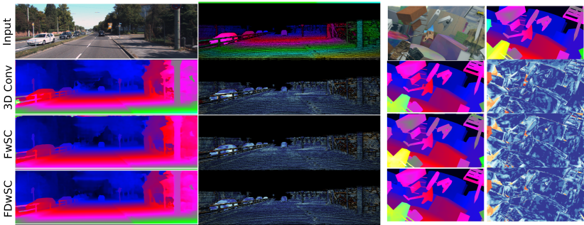
Fig. 3: Qualitative Results of GANet11 model on sample images from KITTI 2015 (left) and SceneFlow (right) datasets. Here the second and fourth columns represent the error maps w.r.t. ground truth. Darker red and blue colors represent higher and lower disparity errors, respectively.

4 Experimental Results

We trained and evaluated our networks on two popular stereo benchmark datasets.
SceneFlow [17] is a large scale synthetic dataset and contains $35,454$ training images and $4,370$ test images of size $540\times 960$ with dense annotations. For our experiments, we further divide the training dataset to $32,454$ training and $3000$ validation pairs following [10] .
KITTI 2015 [24] is a real dataset of driving scenes. It only contains $200$ training and $200$ test image pairs of size $376\times 1240$ pixels with sparse annotations. For our experiments, we further divide the training dataset into $150$ training and $50$ validation pairs as in [10].

4.1 Training Details

For our baseline networks, we use the publicly released code of GANetdeep and PSMNet. For fair comparison and to show the “plug-&-run” capabilities of separable 3D convolutions we use identical training settings for both baseline networks (i.e. networks with 3D convolutions) and optimized networks (i.e. networks with separable 3D convolutions). Furthermore, it is important to mention that we do not perform any type of hyperparameters tuning and train all the networks from scratch (given in Table 3) with default values as in base networks.
GANet: All the input images are cropped to the size of $240\times 528$ while the maximum disparity is set to $192$. Furthermore, all the images are standard normalized using the mean and standard deviation of the training set. For training, we use the Adam Optimizer ($\lambda=1\text{e-}3$, $\beta_{1}=0.9$ and $\beta_{2}=0.999$) with a training batch size of $4$. For KITTI 2015, we transfer learned the models trained on SceneFlow for $650$ epochs with the learning rate reduced to $1\text{e-}4$ after $300$ epochs.
PSMNet: The majority of settings are identical to the baseline except that the images are randomly cropped to $256\times 512$ during training, and we use a batch size of $8$. Moreover, for transfer learning on KITTI 2015 the learning rate is reduced after $200$ epochs.

4.2 Results

For quantitative comparison, following the SceneFlow and KITTI 2015 evaluation protocols, we report three evaluation metrics including $3$-pixels, D1 and End-Point-Errors (EPE) [17, 24] for all the networks . On the SceneFlow dataset (Table 3 (left)) we notice that for most of the cases, networks with FwSCs outperform baseline networks with 3D convolutions despite having around $6.7\times$ less operations and $3.3\times$ fewer parameters. The better performance of FwSCs, compared to 3D convolutions, can be attributed to the fact that a cost volume contains a lot of redundant information (the majority of an image neighbouring disparities do not change) and these separable 3D convolutions contain enough representation power to model disparity variations. Surprisingly, even extremely separable FDwSCs perform better than regular 3D convolutions in most of the cases. However, their performance is a little inferior to FwSC, which is somewhat expected, due to the loss of their correlation modeling capabilities in disparity dimension.

By looking at the quantitative results from the KITTI 2015 dataset from Table 3 (right) we can draw similar conclusions as on the SceneFlow dataset. FwSCs still outperform 3D convolutional networks with a relatively smaller number of 3D convolutional layers, e.g. GANetdeep has $15$ convolutional layers. However, for the networks with a far higher number of 3D convolutional layers, e.g. PSMNet ($22$ convolutional layers) we see a slight deterioration in their performance – this might be because KITTI 2015 is a small and sparse dataset. FDwSCs also give comparable performance to FwSCs and 3D convolutions.

Fig. 3 shows qualitative results on sample examples from the KITTI 2015 validation and SceneFlow test set. Here once again we can verify that separable 3D convolutions are giving comparable results to their 3D convolutions counterparts.

5 Conclusions

In this work, we have shown that 3D convolutional layers are the major bottleneck in overall execution of 3D stereo networks. To circumvent this we have proposed and empirically shown that separable 3D convolutions can considerably reduce the number of operations and parameters for stereo matching in state of the art networks. These proposed convolutions not only lead to leaner networks but they also consistently lead to better performance of these networks. We believe that these convolutions “plug-&-run” nature can lead to their integration into many other 3D stereo networks.

References

- [1] Daniel Scharstein and Richard Szeliski, “A taxonomy and evaluation of dense two-frame stereo correspondence algorithms,” International journal of computer vision, vol. 47, no. 1-3, pp. 7–42, 2002.
- [2] Asmaa Hosni, Christoph Rhemann, Michael Bleyer, Carsten Rother, and Margrit Gelautz, “Fast cost-volume filtering for visual correspondence and beyond,” IEEE TPAMI, vol. 35, no. 2, pp. 504–511, 2012.
- [3] Kuk-Jin Yoon and In So Kweon, “Adaptive support-weight approach for correspondence search,” IEEE TPAMI, vol. 28, no. 4, pp. 650–656, 2006.
- [4] Dongbo Min, Jiangbo Lu, and Minh N Do, “A revisit to cost aggregation in stereo matching: How far can we reduce its computational redundancy?,” in 2011 International Conference on Computer Vision. IEEE, 2011, pp. 1567–1574.
- [5] Jure Žbontar and Yann LeCun, “Stereo Matching by Training a Convolutional Neural Network to Compare Image Patches,” arXiv:1510.05970 [cs], May 2016, arXiv: 1510.05970.
- [6] Akihito Seki and Marc Pollefeys, “SGM-Nets: Semi-Global Matching with Neural Networks,” in 2017 IEEE Conference on Computer Vision and Pattern Recognition (CVPR), Honolulu, HI, July 2017, pp. 6640–6649, IEEE.
- [7] Wenjie Luo, Alexander G Schwing, and Raquel Urtasun, “Efficient deep learning for stereo matching,” in Proceedings of the IEEE CVPR, 2016, pp. 5695–5703.
- [8] Alex Kendall, Hayk Martirosyan, Saumitro Dasgupta, Peter Henry, Ryan Kennedy, Abraham Bachrach, and Adam Bry, “End-to-end learning of geometry and context for deep stereo regression,” 2017.
- [9] Jia-Ren Chang and Yong-Sheng Chen, “Pyramid Stereo Matching Network,” in 2018 IEEE/CVF Conference on Computer Vision and Pattern Recognition, Salt Lake City, UT, June 2018, pp. 5410–5418, IEEE.
- [10] Feihu Zhang, Victor Prisacariu, Ruigang Yang, and Philip H. S. Torr, “GA-Net: Guided Aggregation Net for End-to-end Stereo Matching,” arXiv:1904.06587 [cs], Apr. 2019, arXiv: 1904.06587.
- [11] Yan Wang, Zihang Lai, Gao Huang, Brian H. Wang, Laurens van der Maaten, Mark Campbell, and Kilian Q. Weinberger, “Anytime Stereo Image Depth Estimation on Mobile Devices,” arXiv:1810.11408 [cs], Mar. 2019, arXiv: 1810.11408.
- [12] Stepan Tulyakov, Anton Ivanov, and Francois Fleuret, “Practical deep stereo (pds): Toward applications-friendly deep stereo matching,” 2018.
- [13] Shivam Duggal, Shenlong Wang, Wei-Chiu Ma, Rui Hu, and Raquel Urtasun, “Deeppruner: Learning Efficient Stereo Matching Via Differentiable Patchmatch,” arXiv:1909.05845 [cs], Sept. 2019, arXiv: 1909.05845.
- [14] Zhaofan Qiu, Ting Yao, and Tao Mei, “Learning spatio-temporal representation with pseudo-3d residual networks,” 2017.
- [15] Rongtian Ye, Fangyu Liu, and Liqiang Zhang, “3D Depthwise Convolution: Reducing Model Parameters in 3D Vision Tasks,” arXiv:1808.01556 [cs], Aug. 2018, arXiv: 1808.01556.
- [16] Matteo Poggi, Fabio Tosi, Konstantinos Batsos, Philippos Mordohai, and Stefano Mattoccia, “On the Synergies between Machine Learning and Stereo: a Survey,” arXiv:2004.08566 [cs], Apr. 2020, arXiv: 2004.08566.
- [17] Nikolaus Mayer, Eddy Ilg, Philip Hausser, Philipp Fischer, Daniel Cremers, Alexey Dosovitskiy, and Thomas Brox, “A Large Dataset to Train Convolutional Networks for Disparity, Optical Flow, and Scene Flow Estimation,” in 2016 IEEE Conference on Computer Vision and Pattern Recognition (CVPR), Las Vegas, NV, USA, June 2016, pp. 4040–4048, IEEE.
- [18] Zhengfa Liang, Yiliu Feng, Yulan Guo, Hengzhu Liu, Wei Chen, Linbo Qiao, Li Zhou, and Jianfeng Zhang, “Learning for Disparity Estimation through Feature Constancy,” arXiv:1712.01039 [cs], Mar. 2018, arXiv: 1712.01039.
- [19] Alessio Tonioni, Fabio Tosi, Matteo Poggi, Stefano Mattoccia, and Luigi Di Stefano, “Real-time self-adaptive deep stereo,” arXiv:1810.05424 [cs], Oct. 2018, arXiv: 1810.05424.
- [20] Guorun Yang, Hengshuang Zhao, Jianping Shi, Zhidong Deng, and Jiaya Jia, “SegStereo: Exploiting Semantic Information for Disparity Estimation,” arXiv:1807.11699 [cs], July 2018, arXiv: 1807.11699.
- [21] Xiao Song, Xu Zhao, Hanwen Hu, and Liangji Fang, “EdgeStereo: A Context Integrated Residual Pyramid Network for Stereo Matching,” arXiv:1803.05196 [cs], Sept. 2018, arXiv: 1803.05196.
- [22] Mark Sandler, Andrew Howard, Menglong Zhu, Andrey Zhmoginov, and Liang-Chieh Chen, “Mobilenetv2: Inverted residuals and linear bottlenecks,” in Proceedings of the IEEE CVPR, 2018, pp. 4510–4520.
- [23] Xiangyu Zhang, Xinyu Zhou, Mengxiao Lin, and Jian Sun, “Shufflenet: An extremely efficient convolutional neural network for mobile devices,” in Proceedings of the IEEE CVPR, 2018, pp. 6848–6856.
- [24] Moritz Menze and Andreas Geiger, “Object scene flow for autonomous vehicles,” in 2015 IEEE Conference on Computer Vision and Pattern Recognition (CVPR), Boston, MA, USA, June 2015, pp. 3061–3070, IEEE.