Non-split singularities and conifold transitions in F-theory

Abstract

In F-theory, if a fiber type of an elliptic fibration involves a condition that requires an exceptional curve to split into two irreducible components, it is called “split” or “non-split” type depending on whether it is globally possible or not. In the latter case, the gauge symmetry is reduced to a non-simply-laced Lie algebra due to monodromy. We show that this split/non-split transition is, except for a special class of models, a conifold transition from the resolved to the deformed side, associated with the conifold singularities emerging where the codimension-one singularity is enhanced to $D_{2k+2}$ $(k\geq 1)$ or $E_{7}$. We also examine how the previous proposal for the origin of non-local matter can be actually implemented in our blow-up analysis.

1 Introduction

In F-theory Vafa , singularities play an essential role for the theory to geometrically realize various aspects of string theory MV1 ; MV2 ; BIKMSV ; KatzVafa . An F-theory compactified on an elliptic Calabi-Yau $n$-fold is basically a type IIB theory compactified on an $(n-1)$-dimensional base of a Calabi-Yau manifold with 7-branes in it, where the configuration of the axio-dilaton of type IIB string is described by that of the elliptic modulus of the fibration. A codimension-one locus of the base over which the elliptic fibers become singular is the place where a collection of 7-branes reside on top of each other and typically realizes a non-abelian gauge symmetry depending on the fiber type following Kodaira’s classification. Similarly, a codimension-two locus in the base is involved in matter generation. A codimension-three locus in the base is also possible in four-dimensional F-theory on a Calabi-Yau four-fold, involving Yukawa couplings.

Kodaira’s classification Kodaira of singular fibers of an elliptic surface is based on the intersection diagrams of exceptional curves that arise after the resolutions (table 1). For an elliptic Calabi-Yau $n$-fold which also allows a fibration of an elliptic surface over an $(n-2)$-fold, the singularities of (singular fibers of) these fibered elliptic surfaces are aligned all the way along the $(n-2)$-fold, forming a codimension-two locus in the total elliptic Calabi-Yau $n$-fold, whose projection to the base (of the elliptic fibration) is the “codimension-one” locus mentioned above. We can blow up these “codimension-one” singularities in the base (codimension-two in the total space) to yield a collection of exceptional curves aligned along the “codimension-one” locus, so we can still talk about the fiber type of the singularity over a generic point on the “codimension-one” locus.

Table 1: Kodaira’s classification of singularities of an elliptic surface.

ord$(f)$	ord$(g)$	ord$(\Delta)$	Fiber type	$G$
$\geq 0$	$\geq 0$	$0$	smooth	none
$0$	$0$	$n$	$I_{n}$	$A_{n-1}$
$\geq 1$	$1$	$2$	$II$	none
$1$	$\geq 2$	$3$	$III$	$A_{1}$
$\geq 2$	$2$	$4$	$IV$	$A_{2}$
$2$	$\geq 3$	$n+6$	$I_{n}^{*}$	$D_{n+4}$
$\geq 2$	$3$	$n+6$	$I_{n}^{*}$	$D_{n+4}$
$\geq 3$	$4$	$8$	$IV^{*}$	$E_{6}$
$3$	$\geq 5$	$9$	$III^{*}$	$E_{7}$
$\geq 4$	$5$	$10$	$II^{*}$	$E_{8}$
$\geq 4$	$\geq 6$	$\geq 12$	non-minimal

Table 2: Singularities of the split and non-split types. For the $I_{2k+1}$ fiber type, $I_{2k+1}^{os}$ denotes the “over-split type” which is explained in the text.

$\begin{array}[]{c}\raisebox{-4.30554pt}{Kodaira's}\\ \raisebox{4.30554pt}{fiber type}\\ \end{array}$	ord$(b_{2})$	ord$(b_{4})$	ord$(b_{6})$	ord$(b_{8})$	ord$(\Delta)$	$\begin{array}[]{c}\raisebox{-4.30554pt}{Additional}\\ \raisebox{4.30554pt}{constraint(s)}\\ \end{array}$	$\begin{array}[]{c}\raisebox{-4.30554pt}{Split/non-split}\\ \raisebox{4.30554pt}{fiber type}\\ \end{array}$
$I_{2k}(k\geq 2)$	$0$	$k$	$2k$	$2k$	$2k$	$b_{2,0}=c_{1,0}^{2}$	$I_{2k}^{s}$
						$b_{2,0}$ generic	$I_{2k}^{ns}$
$I_{2k+1}(k\geq 1)$	$0$	$k$	$2k$	$2k+1$	$2k+1$	$\left\{\begin{array}[]{l}b_{2,0}=c_{1,0}^{2}\\ b_{4,k}=c_{1,0}c_{3,k}\\ b_{6,2k}=c_{3,k}^{2}\end{array}\right.$	$I_{2k+1}^{s}$
						$\left\{\begin{array}[]{l}b_{2,0}~{}\mbox{generic}\\ b_{4,k}=b_{2,0}c_{2,k}\\ b_{6,2k}=b_{2,0}c_{2,k}^{2}\end{array}\right.$	$I_{2k+1}^{ns}$
						$\left\{\begin{array}[]{l}b_{2,0}=c_{1,0}^{2}\\ b_{4,k}=c_{1,0}^{2}c_{2,k}\\ b_{6,2k}=c_{1,0}^{2}c_{2,k}^{2}\end{array}\right.$	$I_{2k+1}^{os}$
$I_{0}^{*}$	$1$	$2$	$3$	$4$	$6$	$\left\{\begin{array}[]{l}b_{2,1}=4(p_{2,1}+q_{2,1}+r_{2,1})\\ b_{4,2}=2(p_{2,1}q_{2,1}+q_{2,1}r_{2,1}+r_{2,1}p_{2,1})\\ b_{6,3}=4p_{2,1}q_{2,1}r_{2,1}\end{array}\right.$	$I_{0}^{*s}$
						$\left\{\begin{array}[]{l}b_{2,1}=4(p_{2,1}+q_{2,1})\\ b_{4,2}=2(p_{2,1}q_{2,1}+r_{4,2})\\ b_{6,3}=4p_{2,1}r_{4,2}\end{array}\right.$	$I_{0}^{*ss}$
						$\begin{array}[]{c}\raisebox{-4.30554pt}{$b_{2,1},b_{4,2},b_{6,3}$}\\ \raisebox{4.30554pt}{generic}\end{array}$	$I_{0}^{*ns}$
$I_{2k-3}^{*}\,(k\geq 2)$	$1$	$k+1$	$2k$	$2k+1$	$2k+3$	$b_{6,2k}=c_{3,k}^{2}$	$I_{2k-3}^{*s}$
						$b_{6,2k}$ generic	$I_{2k-3}^{*ns}$
$I_{2k-2}^{*}\,(k\geq 2)$	$1$	$k+1$	$2k+1$	$2k+2$	$2k+4$	$b_{8,2k+2}=c_{4,k+1}^{2}$	$I_{2k-2}^{*s}$
						$b_{8,2k+2}$ generic	$I_{2k-2}^{*ns}$
$IV$	$1$	$2$	$2$	$3$	$4$	$b_{6,2}=c_{3,1}^{2}$	$IV^{s}$
						$b_{6,2}$ generic	$IV^{ns}$
$IV^{*}$	$2$	$3$	$4$	$6$	$8$	$b_{6,4}=c_{3,2}^{2}$	$IV^{*s}$
						$b_{6,4}$ generic	$IV^{*ns}$

In these lower-dimensional F-theories, unlike the eight-dimensional theory on just a single elliptic surface, if the fiber type involves a condition that requires an exceptional curve to split into two irreducible components, these two split curves on a generic point generally meet on top of each other at some point along the “codimension-one” locus. If such exceptional fibers of an elliptic surface constitute part of the same smooth irreducible locus in the total space of the Calabi-Yau, the fiber type is called “non-split” BIKMSV . If this happens, the two apparently distinct exceptional fibers are swapped with each other at some point when one goes along the $(n-2)$-fold, and hence are considered to be identical. This phenomenon is known as a monodromy. The expected $G$ (simply-laced) gauge symmetry is then subject to a projection by a diagram automorphism, reduced to a corresponding non-simply-laced gauge symmetry. Such identification of exceptional fibers can occur when the fiber type is $I_{n}$ $(n=3,4,\ldots)$, $I_{n}^{*}$ $(n=0,1,\ldots)$, $IV$ or $IV^{*}$. If, on the other hand, the two split exceptional fibers of each elliptic surface belong to different irreducible exceptional surfaces in the total Calabi-Yau and hence are split globally, the fiber type is called “split”, yielding the expected $G$ gauge symmetry implied by Kodaira’s classification BIKMSV .

The points where the two exceptional curves overlap constitute a special codimension-two locus in the base space (of the elliptic fibration), where the singularity is enhanced from $G$ to higher in the sense of the fiber type of Kodaira directly over that point. In the split case, there typically (but not always) arises a conifold singularity MT ; EsoleYau , and a wrapped M2-brane (in the M-theory dual) around a new two-cycle, which emerges due to the small resolution, accounts for the generation of the localized matter multiplet KatzVafa .

For example, in a six-dimensional F-theory with $SU(5)$ gauge symmetry compactified on an elliptic Calabi-Yau 3-fold over a Hirzebruch surface $\hbox{\mybb F}_{n}$, there are $n+2$ codimension-two loci on the base where a generic split $I_{5}$ fiber becomes $I_{1}^{*}$, and $3n+16$ loci where it becomes $I_{6}$. Therefore, if a 10 of $SU(5)$ appears at the “$SO(10)$ point” and 5 at the “$SU(6)$ point”, they together with the $5n+36$ neutral hypers from the complex structure moduli exactly satisfy the anomaly cancellation condition $n_{H}-n_{V}=30n+112$ GSWest ; BIKMSV .

On the other hand, in the non-split $I_{5}$ case, while 5’s are still expected to appear at the $SU(6)$ points where the structure of the singularity does not change, the anomaly cancellation condition cannot be satisfied no matter what kind of matter field is assumed to be locally generated at the $SO(10)$ points, which are twice as many as the split case. On top of that, the conifold singularity does not appear, even though the singularity in the sense of Kodaira is apparently enhanced to $SO(10)$ over that point. Rather, by blowing up a nearby “codimension-one” singularity, the singularity there is simultaneously resolved together. Thus there is no sign of a localized matter field in the non-split case, although the anomaly cancellation condition (in six dimensions in particular) requires a definite amount of chiral matter field to arise even in the non-split model with a non-simply-laced gauge symmetry. Such a phenomenon is widespread in other non-split models BIKMSV ; AKM ; GHLST ; AGW ; EJK ; EK ; EJ .

In fact, Ref. AKM has proposed a mechanism for non-local matter generation that does not require any new exceptional curves in those non-split models. The idea is as follows: As mentioned above, in a non-split model, some of the exceptional curves are identified in pairs. Each such pair forms a ruled (=$\hbox{\mybb P}^{1}$-fibered) (complex) surface whose base is a (real two-dimensional) Riemann surface of genus $g$, where $2g+2$ is the number of the places where the conifold singularities disappear on the gauge divisor in the transition to the non-split model. According to Witten’s and Katz-Morrison-Plesser(KMP)’s discussions Witten ; KMP , they claim that from each pair there appear $g$ hypermultiplets from (the harmonic 1-forms of) the genus-$g$ Riemann surface, corresponding to a short simple root of the non-simply-laced gauge Lie algebra of the non-split model. It was argued that all these hypermultiplets, together with ones coming from the monodromy-invariant exceptional curves, generate the whole desired representation at the desired multiplicities AKM .

This proposal works well, but some questions remain:
(1) In split models, conifold singularities appear, and hypermultiplets are generated from their small resolutions. On the other hand, AKM proposed that hypermultiplets appear from the genus-$g$ Riemann surface. Are they related, and if so, how?
(2) AKM is based on Witten’s and KMP’s discussions of hypermultiplet generation, but in the latter the situation is that there is originally a genus-$g$ Riemann surface with a singularity on it, whereas in the present case the gauge divisor is genus-zero. (That is consistent with the spectrum not including the adjoint hyper.) Certainly a blow-up gives rise to a ruled surface on a genus-$g$ Riemann surface, but if there are multiple pairs of exceptional curves that are identified by monodromy, it appears that multiple ruled surfaces on different genus-$g$ Riemann surfaces arise. Can we still in that case apply AKM ’s argument which assumes only a single Riemann surface of genus $g$?

In this paper, we perform blow-ups in all models where there is a distinction between split and non-split fiber types, and by doing so we specifically examine the proposal of AKM for non-local generation of matter fields in the non-split models of F-theory . We will deal with a 6D F-theory compactified on an elliptic Calabi-Yau threefold (and stable degenerations thereof) on the Hirzebruch surface MV1 ; MV2 ; BIKMSV . We will show that the split/non-split transition is, except for some special cases, a conifold transition CdlOGP ; CGH ; CdlO ; CdlO2 ; AGM ; Strominger from the resolved to the deformed side, associated with conifold singularities emerging at codimension-two loci in the base of the split models. The “genus-$g$ curve” of AKM can be obtained as an intersection of this local deformed conifold and some appropriate divisors. This will answer the question (1).

It turns out that there are several different patterns of the transition. We found that, at the codimension-two loci of the base where the relevant conifold singularities arise after the codimension-one blow-ups, the singularity there is always enhanced to $D_{2k+2}$ ($k\geq 1$), or $E_{7}$ which is the only case for the $IV^{*s}\leftrightarrow IV^{*ns}$ transition, except for a special class of models in which no conifold singularity appears at the relevant codimension-two singularity in the split models. We will also show that the $I_{2k+1}$ split models ($k\geq 1$), which do not generically have the $D_{2k+2}$ enhanced points, do not transition directly to $I_{2k+1}$ non-split models, but do via special $I_{2k+1}$ split models where the complex structure is tuned in such a way that they may develop $D_{2k+2}$ enhanced points. We will refer to these specially tuned split models as “over-split” models and denote them by $I_{2k+1}^{os}$.

In all these cases where a conifold transition occurs, the conifold singularities are resolved in the split models by small resolutions to yield exceptional curves which are two-cycles. Thus the split models are on the resolved side of the conifold transition. On the other hand, we will show that modifying the sections relevant to the transition from the split to the non-split model amounts to deforming the conifold singularities to yield local deformed conifolds, where three-cycles appear instead of two-cycles on the resolved (split) side.

We will explicitly show the equation of the genus-$g$ curve for each pair of exceptional curves that join smoothly at a branch point of it represented as a 2-sheeted Riemann surface. Since such a complex two-surface “swept” by a pair of curves constitutes a root of the non-simply-laced gauge Lie algebra and arises at each step of the blow-up, a priori the genus-$g$ base could be different for each pair if there is more than one pair of exceptional curves that are identified (in the cases of $C_{k}$ and $F_{4}$). If so, that would be a problem, since AKM assumes the existence of only one genus-$g$ base (“$M_{2}$” in AKM ), whose zero modes are responsible for the generation of the necessary hypermultiplets. Happily, we show that the genus-$g$ bases are all identical and common in these cases, so we can have a well-defined single genus-$g$ base for these cases as well. This is the answer to the question (2).

The rest of this paper is organized as follows. In section 2, we summarize the basic set-ups of 6D F-theory on an elliptic Calabi-Yau threefold over a Hirzebruch surface, which will be used in the subsequent sections. Sections 3 to 7 consider separately all fiber types in which a non-split type exists. We deal with the $I_{2k}$ models first in section 3, and show in detail that the split/non-split transition there is a conifold transition associated with the conifold singularities arising at the $D_{2k}$ points. The last subsection gives a short summary of the proposal of AKM for non-local matter generation and answer to the questions stated above. The fiber types $I_{2k+1}$, $IV$ and $IV^{*}$ are studied in sections 4,5 and 6, respectively, and a similar conclusion is reached, with an exception that the relevant conifold transition occurs at the $E_{7}$ points in the $IV^{*}$ model. Section 7 is devoted to the study of the final example, the $I_{n}^{*}$ models, where it is shown that in the $I_{2k-3}^{*}$ models, the split/non-split transition is similarly understood as a conifold transition, while in the $I_{2k-2}^{*}$ models, no conifold singularity arises at the relevant enhanced points. Finally, we conclude in section 8.

2 Summary of 6D F-theory on an elliptic Calabi-Yau threefold over a Hirzebruch surface

Let us consider six-dimensional F-theory compactified on an elliptic Calabi-Yau threefold $Y_{3}$ with a section fibered over a Hirzebruch surface $\hbox{\mybb F}_{n}$ ($n\geq 0$) MV1 ; MV2 . We define $Y_{3}$ as a hypersurface

$$-(y^{2}+a_{1}xy+a_{3}y)+x^{3}+a_{2}x^{2}+a_{4}x+a_{6}=0$$ (1)

in a complex four-dimensional ambient space $X_{4}$, which itself is a $\hbox{\mybb P}^{2}$ fibration over $\hbox{\mybb F}_{n}$. $(x,y)$ are the affine coordinates in a coordinate patch of $\hbox{\mybb P}^{2}$ where one of the homogeneous coordinates does not vanish and hence is set to 1. Let ${\cal K}$ be the canonical bundle of $\hbox{\mybb F}_{n}$, then $x$, $y$ are sections of ${\cal K}^{-2}$, ${\cal K}^{-3}$, whereas $a_{j}$ $(j=1,2,3,4,6)$ are ones of ${\cal K}^{-j}$, respectively, so that the hypersurface (1) defines a Calabi-Yau threefold.

A Hirzebruch surface $\hbox{\mybb F}_{n}$ is a $\hbox{\mybb P}^{1}$ fibration over $\hbox{\mybb P}^{1}$, defined as a toric variety with the following toric charges

(5)

$(u^{\prime}:v^{\prime})$ are the homogeneous coordinates of the base $\hbox{\mybb P}^{1}$, while $(u:v)$ are the ones of the fiber $\hbox{\mybb P}^{1}$. The anti-canonical bundle corresponds to the divisor $(n+2)D_{u^{\prime}}+2D_{v}$, where we denote, for a given coordinate $X$, by $D_{X}$ a divisor defined by the zero locus $X=0$. Thus, if we define affine coordinates $z\equiv\frac{u}{v}$, $w\equiv\frac{u^{\prime}}{v^{\prime}}$ in a patch $v\neq 0$ and $v^{\prime}\neq 0$, the section $a_{j}$ is given as a $2j$th degree polynomial in $z$ and a $j(n+2)$th degree polynomial in $w$.

The hypersurface so defined is also a K3 fibration, the base of which is the base $\hbox{\mybb P}^{1}$ of $\hbox{\mybb F}_{n}$. We next consider the stable degeneration limit of this K3. Schematically, this is regarded as a limit of splitting into a pair of rational elliptic surfaces ${\rm dP}_{9}$ glued together along the torus fiber over the “infinite points” of the respective bases. See MV2 ; Aspinwall for a more rigorous definition.

It is convenient to move on to a ${\rm dP}_{9}$ fibration over the same $\hbox{\mybb P}^{1}$ with $u^{\prime},v^{\prime}$ being its coordinates. To do this, we have only to change the divisor class of $a_{j}$ from $j((n+2)D_{u^{\prime}}+2D_{v})$ ($=$ the divisor of ${\cal K}^{-j}$) to

$$j((n+2)D_{u^{\prime}}+D_{v}).$$ (6)

With this change, $a_{j}$ is still a $j(n+2)$th degree polynomial in $w$ but becomes $j$th degree in $z$. Likewise, the divisor classes of $x$ and $y$ are modified from $2((n+2)D_{u^{\prime}}+2D_{v})$, $3((n+2)D_{u^{\prime}}+2D_{v})$ to

$$2((n+2)D_{u^{\prime}}+D_{v}),~{}~{}3((n+2)D_{u^{\prime}}+D_{v}),$$ (7)

respectively. This ${\rm dP}_{9}$ fiber describes one $E_{8}$ of the $E_{8}\times E_{8}$ gauge symmetry. The terms of degrees from $j+1$ to $2j$ appearing in $a_{j}$ for the K3 fibration correspond to the other ${\rm dP}_{9}$ residing “beyond the infinity”. For generic ${\rm dP}_{9}$ fibrations, $a_{j}$ is expanded as

$$a_{j}=a_{j,0}+a_{j,1}z+\cdots+a_{j,j-1}z^{j-1}+a_{j,j}z^{j}~{}~{}~{}(j=1,2,3,4,6),$$ (8)

then the section $a_{j,k}$ of each coefficient becomes a ($(j-k)n+2j$)th degree polynomial in $w$ due to the nonzero $Q^{1}$ charge carried by $u$.

As an equation of an elliptic fiber, (1) is commonly referred to as “Tate’s form”. One can complete the square with respect to $y$ in (1) to obtain (with a redefinition of $y$)

$$-y^{2}+x^{3}+\frac{b_{2}}{4}x^{2}+\frac{b_{4}}{2}x+\frac{b_{6}}{4}=0,$$ (9)

$$b_{2} = a_{1}^{2}+4a_{2},$$

$$b_{4} = a_{1}a_{3}+2a_{4},$$ (10)

$$b_{6} = a_{3}^{2}+4a_{6},$$

which, though less common, we call the “Deligne form” in this paper Deligne . $b_{j}$ is a section of the same line bundle as $a_{j}$ and similarly expanded as

$$b_{j}=b_{j,0}+b_{j,1}z+\cdots+b_{j,j-1}z^{j-1}+b_{j,j}z^{j}~{}~{}~{}(j=2,4,6),$$ (11)

where $b_{j,k}$ is also a ($(j-k)n+2j$)th degree polynomial in $w$. It is also convenient to define BIKMSV

$$b_{8} = \frac{1}{4}(b_{2}b_{6}-b_{4}^{2}),$$ (12)

which is the (minus of the) discriminant of the quadratic equation

$$\frac{b_{2}}{4}x^{2}+\frac{b_{4}}{2}x+\frac{b_{6}}{4}=0$$ (13)

of $x$.

Finally, one can “complete the cube” with respect to $x$ in (9) and find (with a redefinition of $x$)

$$-y^{2}+x^{3}+fx+g=0,$$ (14)

$$f = -\frac{1}{48}(b_{2}^{2}-24b_{4}),$$

$$g = \frac{1}{864}\left(b_{2}^{3}-36b_{2}b_{4}+216b_{6}\right),$$ (15)

which is called the “Weierstrass form”. $f$ and $g$ are sections of the same line bundle as $a_{4}$ and $a_{6}$, respectively, and in the ${\rm dP}_{9}$ fibration they are expanded as

$$f = f_{4,0}+f_{4,1}z+\cdots+f_{4,4}z^{4},$$

$$g = g_{6,0}+g_{6,1}z+\cdots+g_{6,6}z^{6},$$ (16)

where $f_{4,k}$, $g_{6,k}$ are written as $f_{(4-k)n+8}$, $g_{(6-k)n+12}$ in MV1 , whose degrees in $w$ are specified by their subscripts. The discriminant $\Delta$ of (14) is

$$\Delta = 4f^{3}+27g^{2}$$ (17)

$$= \frac{1}{16}\left(b_{2}^{2}b_{8}-9b_{2}b_{4}b_{6}+8b_{4}^{3}+27b_{6}^{2}\right).$$

Consider the case where the elliptic fiber over $z=0$ of the base $\hbox{\mybb P}^{1}$ of this ${\rm dP}_{9}$ (i.e. the fiber $\hbox{\mybb P}^{1}$ of the $\hbox{\mybb F}_{n}$) has a singularity, and the exceptional fibers after the resolution fall into one of Kodaira’s fiber types. It is well-known that the fiber type of a given singularity is determined in terms of the vanishing orders of the sections $f$, $g$ of the Weierstrass form as well as the discriminant $\Delta$ (table 1).

Note that, in Kodaira’s classification, there is no upper limit on the vanishing orders of $f$, $g$ or $\Delta$ (since any large value of $n$ is allowed for the fiber type $I_{n}$ or $I^{*}_{n}$ as a fiber type) , but there is when we try to realize singular fibers in a ${\rm dP}_{9}$ fibration. Since the relationship between the split/non-split transition and the conifold transition discussed below is also a local one in the sense that it does not depend on another singularity located far away, we will also need to consider a high vanishing order that cannot be realized in a ${\rm dP}_{9}$ fibration. So in this paper, we will first start from a ${\rm dP}_{9}$ fibration and consider heterotic duality when it makes sense, while discussing the relationship between the two transitions locally in the same set-up even when the fiber cannot be realized in a ${\rm dP}_{9}$ fibration.

As we already described in Introduction, if the type of a singular fiber is either $I_{n}$ $(n=3,4,\ldots)$, $I_{n}^{*}$ $(n=0,1,\ldots)$, $IV$ or $IV^{*}$ at a generic point $w$ on the divisor $z=0$ in $\hbox{\mybb F}_{n}$, it is further classified as a split type or a non-split type, depending on whether or not the split condition is satisfied globally . We have listed them in table 2 together with the required constraints for the fibers to be classified into the respective types . In the following, we will study these individual cases.

3 Split/non-split transitions as conifold transitions (I): the $I_{2k}$ models

3.1 Generalities of the $I_{n}$ models

Let us first summarize the generalities of the $I_{n}$ models common to both cases when $n$ is even and when $n$ is odd . As displayed in table 2, the vanishing orders of the sections $b_{2}$, $b_{4}$ and $b_{6}$ of (9) are $(0,k,2k)$ for both $I_{2k}$ and $I_{2k+1}$. The only difference is that the order of $b_{8}$ (12) is the generic value $2k$ in the $I_{2k}$ type, while in the $I_{2k+1}$ type $b_{2}$, $b_{4}$ and $b_{6}$ take special values so that the order of $b_{8}$ goes up to $2k+1$. Explicitly, the equation of these models is given by

$$\Phi(x,y,z,w)\equiv -y^{2}+x^{3} +{\textstyle\frac{1}{4}}(b_{2,0}+b_{2,1}z+\cdots)x^{2}$$ (18)

$$+{\textstyle\frac{1}{2}}(b_{4,k}z^{k}+b_{4,k+1}z^{k+1}+\cdots)x$$

$$+{\textstyle\frac{1}{4}}(b_{6,2k}z^{2k}+b_{6,2k+1}z^{2k+1}+\cdots)=0.$$

As mentioned at the end of the previous section, this equation is not well defined as a ${\rm dP}_{9}$ fibration when $k$ is large (e.g., $k\geq 4$), but even in that case we will use it to analyze the local structure near the conifold singularities associated with the split/non-split transition.

The equation (18) has a singularity at $(x,y,z)=(0,0,0)$ for arbitrary $w$ in both cases. We will blow up this singularity, as well as the ones we will subsequently encounter, by taking the usual steps. Let us explain the general procedure of how this is done by taking the present case as an example. Our notation is similar to the one used in our previous paper KMT .

We first replace the point $(x,y,z)=(0,0,0)$ in the complex three-dimensional $(x,y,z)$ space, which is a local patch of the three-dimensional ambient space defining the ${\rm dP}_{9}$, by a $\hbox{\mybb P}^{2}$ by replacing $\hbox{\mybb C}^{3}\ni(x,y,z)$ with

$$\hat{\hbox{\mybb C}}^{3} = \{((x,y,z),(\xi:\eta:\zeta))\in\hbox{\mybb C}^{3}\times\hbox{\mybb P}^{2}~{}|~{}(x:y:z)=(\xi:\eta:\zeta)\}.$$ (19)

We work in inhomogeneous coordinates defined in three different patches of this $\hbox{\mybb P}^{2}$

$$(x:y:z)=(\xi:\eta:\zeta) = (1:y_{1}:z_{1})~{}~{}~{}\mbox{(${\bf 1}_{x}$, $x\neq 0$),}$$ (20)

$$= (x_{1}:1:z_{1})~{}~{}~{}\mbox{(${\bf 1}_{y}$, $y\neq 0$),}$$

$$= (x_{1}:y_{1}:1)~{}~{}~{}\mbox{(${\bf 1}_{z}$, $z\neq 0$)},$$

where ${\bf 1}_{x}$, ${\bf 1}_{y}$ and ${\bf 1}_{z}$ are the names of the coordinate patches. Then replacing $\hbox{\mybb C}^{3}$ with $\hat{\hbox{\mybb C}}^{3}$ (19) is simply achieved by replacing $(x,y,z)$ with $(x,xy_{1},xz_{1})$ in ${\bf 1}_{x}$, $(x_{1}y,y,yz_{1})$ in ${\bf 1}_{y}$ and $(x_{1}z,y_{1}z,z)$ in ${\bf 1}_{z}$ in the equation (18), respectively, followed by dividing by the square of the scale factor

$$x^{-2}\Phi(x,xy_{1},xz_{1},w)\equiv\Phi_{x}(x,y_{1},z_{1},w)=0~{}~{}~{}\mbox{(${\bf 1}_{x}$),}$$

$$y^{-2}\Phi(x_{1}y,y,yz_{1},w)\equiv\Phi_{y}(x_{1},y,z_{1},w)=0~{}~{}~{}\mbox{(${\bf 1}_{y}$),}$$

$$z^{-2}\Phi(x_{1}z,y_{1}z,z,w)\equiv\Phi_{z}(x_{1},y_{1},z,w)=0~{}~{}~{}\mbox{(${\bf 1}_{z}$)}$$ (21)

so as not to change the canonical class.

Then we see that, unless $k=1$ ($I_{2}$ and $I_{3}$), another singularity appears in the patch ${\bf 1}_{z}$ at $(x_{1},y_{1},z)=(0,0,0)$, then we do a similar replacement and factorization

$$x_{1}^{-2}\Phi_{z}(x_{1},x_{1}y_{2},x_{1}z_{2},w)\equiv\Phi_{zx}(x_{1},y_{2},z_{2},w)=0~{}~{}~{}\mbox{(${\bf 2}_{zx}$),}$$

$$y_{1}^{-2}\Phi_{z}(x_{2}y_{1},y_{1},y_{1}z_{2},w)\equiv\Phi_{zy}(x_{2},y_{1},z_{2},w)=0~{}~{}~{}\mbox{(${\bf 2}_{zy}$),}$$

$$z^{-2}\Phi_{z}(x_{2}z,y_{2}z,z,w)\equiv\Phi_{zz}(x_{2},y_{2},z,w)=0~{}~{}~{}\mbox{(${\bf 2}_{zz}$).}$$ (22)

for each patch of another $\hbox{\mybb P}^{2}$ put at $(x_{1},y_{1},z)=(0,0,0)$. Again, if $k$ is larger than two, we find a singularity in the patch ${\bf 2}_{zz}$, which we blow up to obtain $\Phi_{zzz}(x_{3},y_{3},z,w)$. Repeating these steps $k$ times yields $\Phi_{\underbrace{\mbox{\scriptsize$z\cdots z$}}_{k}}(x_{k},y_{k},z,w)$, the properties of which differ between the types $I_{2k}$ and $I_{2k+1}$.

In the following, we will use the following $j$-times blown-up equations recursively defined by

$$z^{-2}\Phi_{\underbrace{\mbox{\scriptsize$z\cdots z$}}_{j-1}}(x_{j}z,y_{j}z,z,w) \equiv \Phi_{\underbrace{\mbox{\scriptsize$z\cdots z$}}_{j}}(x_{j},y_{j},z,w)=0~{}~{}~{}(\mbox{\boldmath$j$}_{\underbrace{\mbox{\scriptsize$z\cdots z$}}_{j}}),$$ (23)

$$x_{j-1}^{-2}\Phi_{\underbrace{\mbox{\scriptsize$z\cdots z$}}_{j-1}}(x_{j-1},x_{j-1}y_{j},x_{j-1}z_{j},w) \equiv \Phi_{\underbrace{\mbox{\scriptsize$z\cdots z$}}_{j-1}x}(x_{j-1},y_{j},z_{j},w)=0~{}~{}~{}(\mbox{\boldmath$j$}_{\underbrace{\mbox{\scriptsize$z\cdots z$}}_{j-1}x})$$ (24)

from the $(j-1)$-times blown-up equation $\Phi_{\underbrace{\mbox{\scriptsize$z\cdots z$}}_{j-1}}(x_{j-1},y_{j-1},z,w)=0$ defined in the coordinate patch $\mbox{\boldmath$(j\!-\!1)$}_{\underbrace{\mbox{\scriptsize$z\cdots z$}}_{j-1}}$. (Again, $y_{j}$’s in (23) and (24) are different.)

3.2 “Codimension-one” singularities of the $I_{n}$ models

We have seen in the previous subsection that there appears a singularity in ${\bf 1}_{z}$ at $(x_{1},y_{1},z)=(0,0,0)$ for arbitrary $w$, and after the blow-up there is, if $k\geq 3$, another at $(x_{2},y_{2},z)=(0,0,0)$ in ${\bf 2}_{zz}$ for arbitrary $w$. These singular “points” in the sense of Kodaira are aligned along the base $\hbox{\mybb P}^{1}$ of $\hbox{\mybb F}_{n}$, and hence form complex one-dimensional curves. If, though not considered in this paper, our set-up is generalized to a 4D F-theory compactification where the ${\rm dP}_{9}$ is fibered on some complex two-dimensional base, these singularities are aligned to form complex surfaces. Thus, in this paper, we will call such a singularity in the sense of Kodaira, that forms a codimension-one locus when projected onto the base of the elliptic fibration, a “codimension-one” singularity.

Using this terminology, we can say that, in the process of blowing up, both the $I_{2k}$ and $I_{2k+1}$ models yield a “codimension-one” singularity $p_{j}$ at $(x_{j},y_{j},z,w)=(0,0,0,w)$ for every $j=0,\ldots,k-1$ in ${\mbox{\boldmath$j$}}_{\underbrace{\mbox{\scriptsize$z\cdots z$}}_{j}}$, where we define $(x_{0},y_{0},z,w)\equiv(x,y,z,w)$. The explicit form of $\Phi_{\underbrace{\mbox{\scriptsize$z\cdots z$}}_{j}}(x_{j},y_{j},z,w)$ representing the model in this patch is given by

$$\Phi_{\underbrace{\mbox{\scriptsize$z\cdots z$}}_{j}}(x_{j},y_{j},z,w) = -y_{j}^{2}+x_{j}^{3}z^{j}+{\textstyle\frac{1}{4}}(b_{2,0}+b_{2,1}z+\cdots)x_{j}^{2}$$

$$+{\textstyle\frac{1}{2}}(b_{4,k}z^{k-j}+b_{4,k+1}z^{k-j+1}+\cdots)x_{j}$$

$$+{\textstyle\frac{1}{4}}(b_{6,2k}z^{2(k-j)}+b_{6,2k+1}z^{2(k-j)+1}+\cdots)$$

$$\stackrel{{\scriptstyle z\rightarrow 0}}{{\rightarrow}} -y_{j}^{2}+{\textstyle\frac{1}{4}}b_{2,0}x_{j}^{2}$$

where the exceptional “curve” (in the $\hbox{\mybb P}^{2}$ blown up over some point of the base with fixed (generic) $w$) splits into two lines in the sense of Kodaira. Thus, for each generic $w$, $p_{j}$ is located at the intersection point of these exceptional curves that have arisen from blowing up $p_{j-1}$ $(j=1,\ldots,k-1)$. Blowing up the final singularity $p_{k-1}$ yields a single irreducible exceptional curve for the $I_{2k}$ case, and a pair of split lines for the $I_{2k+1}$ case (see figures 1,2 ). Putting them all together, they constitute the $A_{2k-1}$ and $A_{2k}$ Dynkin diagrams as their intersection diagrams, as is well known.

3.3 Conifold singularities associated with the split/non-split transition in the $I_{2k}$ models

Now let us explain what “conifold singularities associated with the split/non-split transition” are, by taking $I_{2k}$ models as an example. Since there is no distinction between split and non-split fiber types in the fiber type $I_{2}$, let us consider $I_{2k}$ for $k\geq 2$.

The equation of the split $I_{2k}$ model for $k\geq 2$ is given by the equation (18) with

$$b_{2,0}=c_{1,0}^{2}$$ (26)

for some section $c_{1,0}$. A split $I_{2k}$ model exhibits, in addition to these “codimension-one” singularities, conifold singularities on singular fibers over some special loci on the base of the elliptic fibration, where the generic $A_{n-1}$ singularity is enhanced to some higher-rank one.

The discriminant of (18) with (26) reads

$$\Delta = \frac{1}{16}c_{1,0}^{4}b_{8,2k}z^{2k}+\cdots.$$ (27)

$f$ and $g$ (15) derived from (18) are

$$f = -\frac{1}{48}c_{1,0}^{4}+\cdots,$$

$$g = \frac{1}{864}c_{1,0}^{6}+\cdots.$$ (28)

(27) shows that at the zero loci of $c_{1,0}$ and $b_{8,2k}$, the singularity is enhanced from $A_{2k-1}$. Since (28) implies that the vanishing orders of $f$ and $g$ are unchanged at the zero loci of $b_{8,2k}$, they are “$A_{2k}$ points”, which means that they are the places on the base over which the singularities of the fibers are enhanced to $A_{2k}$. On the other hand, at the zero loci of $c_{1,0}$, it turns out that the vanishing orders of $f$ , $g$ and $\Delta$ go up to two, three and $2k+2$, so the zero loci of $c_{1,0}$ are “$D_{2k}$ points”, which similarly means that the singularities are enhanced to $D_{2k}$ there. In fact, they are singularities of the type of the “complete resolution” MT , meaning that they develop the necessary amount of conifold singularities to yield the degrees of freedom of matter hypermultiplets arising there. Thus, according to the general rule KatzVafa , the zero loci of $b_{8,2k}$ are the places (on the base) where a hypermultiplet transforming in ${\bf 2k}$ of $A_{2k-1}$ arises, and those of $c_{1,0}$ are where a hypermultiplet in ${\bf k(2k-1)}$ appears. In general, a section $c_{i,j}$ or $b_{i,j}$ or whatever with a subscript $(i,j)$ is expressed as a polynomial of degree $(i-j)n+2i$ in $w$ MizoguchiTaniLooijenga , so we have $(8-2k)n+16$ hypermultiplets in the ${\bf 2k}$ representation, and $n+2$ hypermultiplets in the ${\bf k(2k-1)}$ representation.

We will focus on the singularity enhancement to $D_{2k}$ at the zero loci of $c_{1,0}$ since it is this singularity enhancement that its associated conifold singularities and their transitions are closely related to the split/non-split transitions in F-theory. Indeed, if we do not impose the condition (26) to (18), we have an equation of the non-split $I_{2k}$ model, for which the corresponding $f$, $g$ and $\Delta$ are the ones obtained by simply replacing every $c_{1,0}^{2}$ with $b_{2,0}$ in (28) and (27). Even then, the vanishing orders of $f$, $g$ and $\Delta$ at the zero loci of $b_{2,0}$ remain the same as those at the loci of $c_{1,0}$, which means that the number of $D_{2k}$ points is doubled ($b_{2,0}$ is represented as a polynomial of degree $2n+4$ in $w$).

Of course, in this process of the transition from the split model to the non-split one, the $D_{2k}$ points, which have doubled in number, cannot continue to produce ${\bf k(2k-1)}$’s after the transition to the non-split side; they are too many to satisfy the anomaly cancellation condition. Therefore, the structure of the conifold singularities that existed before the transition to the non-split model must change after the transition. They are what we call the conifold singularities associated with the split/non-split transition. In contrast, singularity structures of the fibers over the $A_{2k}$ points at which $b_{8,2k}$ vanishes do not change by the replacement $c_{1,0}^{2}\leftrightarrow b_{2,0}$.

3.4 Conifold singularities in the split $I_{2k}$ models for $k\geq 3$

To show how these conifold singularities arise at the $D_{2k}$ points in the blowing-up process of the split $I_{2k}$ models, let us consider the $j$-times blown-up equation $\Phi_{\underbrace{\mbox{\scriptsize$z\cdots z$}}_{j-1}x}(x_{j-1},y_{j},z_{j},w)=0$ in the patch ${\mbox{\boldmath$j$}}_{\underbrace{\mbox{\scriptsize$z\cdots z$}}_{j-1}x}$ for $j=2,\ldots,k-1$ with $k\geq 3$ which is recursively defined in (24) in section 3.1. $k=2$ ($I_{4}$) is a special case, so we will consider it separately in the next subsection.

The left-hand side of this equation is explicitly given by

$$\Phi_{\underbrace{\mbox{\scriptsize$z\cdots z$}}_{j-1}x}(x_{j-1},y_{j},z_{j},w) = -y_{j}^{2}+x_{j-1}^{j}z_{j}^{j-1}$$

$$+{\textstyle\frac{1}{4}}(c_{1,0}^{2}+b_{2,1}x_{j-1}z_{j}+\cdots)$$

$$+{\textstyle\frac{1}{2}}x_{j-1}^{k-j}z_{j}^{k-j+1}(b_{4,k}+b_{4,k+1}x_{j-1}z_{j}+\cdots)$$

$$+{\textstyle\frac{1}{4}}x_{j-1}^{2(k-j)}z_{j}^{2(k-j+1)}(b_{6,2k}+b_{6,2k+1}x_{j-1}z_{j}+\cdots)$$

$$= -y_{j}^{2}+{\textstyle\frac{1}{4}}c_{1,0}^{2}+x_{j-1}z_{j}\left(\rule{0.0pt}{10.76385pt}x_{j-1}^{j-1}z_{j}^{j-2}+{\textstyle\frac{1}{4}}b_{2,1}\right.$$

$$\left.+{\textstyle\frac{1}{2}}b_{4,k}x_{j-1}^{k-j-1}z_{j}^{k-j}+{\textstyle\frac{1}{4}}b_{6,2k}x_{j-1}^{2(k-j)-1}z_{j}^{2(k-j)+1}+O(x_{j-1}z_{j})\right).$$

In general, a conifold is defined in $\hbox{\mybb C}^{4}\ni(z_{1},z_{2},z_{3},z_{4})$ by the equation

$$z_{1}z_{4}+z_{2}z_{3}=0,$$ (30)

where $(z_{1},z_{2},z_{3},z_{4})=(0,0,0,0)$ is the conifold singularity. Thus (LABEL:PhizzzxI2k) shows that the geometry near $y_{j}=c_{1,0}=x_{j-1}=z_{j}=0$ is locally approximated by that of a conifold, and the point itself is the conifold singularity for each $j=2,\ldots,k-1$ ($k\geq 3$).

Since these $k-2$ conifold singularities arise in the blowing-up process of a split $I_{2k}$ model at each zero locus of $c_{1,0}$, the number of which is $n+2$ in total in the present $\hbox{\mybb F}_{n}$ case (because $c_{1,0}$ is a polynomial of degree $n+2$; see subsection 3.3.). Let us pay attention to a particular zero of this $c_{1,0}$, and we can take it to $w=0$ without loss of generality. That is,

$$c_{1,0}=w+O(w^{2})$$ (31)

near $w=0$. Then we see from (LABEL:PhizzzxI2k) that the equation $\Phi_{\underbrace{\mbox{\scriptsize$z\cdots z$}}_{j-1}x}(x_{j-1},y_{j},z_{j},w)=0$ near $(x_{j-1},y_{j},z_{j},w)=(0,0,0,0)$ is

$$-y_{j}^{2}+{\textstyle\frac{1}{4}}w^{2}+\mbox{(const.$\times$)}x_{j-1}z_{j} = 0$$ (32)

up to higher-order terms. The first two terms are factorized to yield the standard conifold equation (30).

The equation (32) tells us that it is precisely the fact that the section $b_{2,0}$ is in the form of a square $c_{1,0}^{2}$ that the blown-up equations $\Phi_{\underbrace{\mbox{\scriptsize$z\cdots z$}}_{j-1}x}(x_{j-1},y_{j},z_{j},w)=0$ give rise to conifold singularities. If $b_{2,0}$ were not in square form $c_{1,0}^{2}$, which implies that the model is non-split, (LABEL:PhizzzxI2k) would be

$$\Phi_{\underbrace{\mbox{\scriptsize$z\cdots z$}}_{j-1}x}(x_{j-1},y_{j},z_{j},w) = -y_{j}^{2}+{\textstyle\frac{1}{4}}b_{2,0}+x_{j-1}z_{j}\left(\cdots\right),$$ (33)

in which $b_{2,0}$ generically vanishes like $w$ near $w=0$, and the corresponding local equation would be

$$-y_{j}^{2}+{\textstyle\frac{1}{4}}w+\mbox{(const.$\times$)}x_{j-1}z_{j} = 0$$ (34)

up to higher-order terms, which is not a conifold equation.

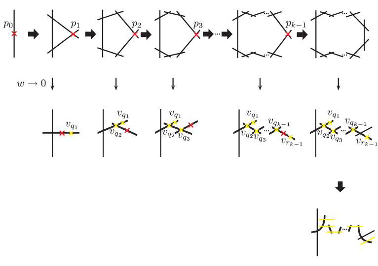
Figure 1: Singularities and exceptional curves arising in the blow-up of a split $I_{2k}$ model near a $D_{2k}$ point $w=0$. “Codimension-one” singularities and conifold singularities are depicted with red and yellow x’s, respectively. Each bold horizontal arrow indicates a blow-up at a “codimension-one” singularity, and the final thick downward arrow means small resolutions of all the conifold singularities. The thin downward arrows denote the $w\rightarrow 0$ limit. The left-most vertical line in each figure represents the original singular fiber.

In the following, we will refer to the $k-2$ conifold singularities arising at each zero locus of $c_{1,0}$ as

$$v_{q_{2}}: (x_{1},y_{2},z_{2},w)=(0,0,0,0)~{}~{}~{}({\mbox{\boldmath$2$}}_{zx}),$$

$$\vdots$$

$$v_{q_{j}}: (x_{j-1},y_{j},z_{j},w)=(0,0,0,0)~{}~{}~{}({\mbox{\boldmath$j$}}_{\underbrace{\mbox{\scriptsize$z\cdots z$}}_{j-1}x}),$$

$$\vdots$$

$$v_{q_{k-1}}: (x_{k-2},y_{k-1},z_{k-1},w)=(0,0,0,0)~{}~{}~{}({\mbox{\boldmath$(\!k-1\!)$}}_{\underbrace{\mbox{\scriptsize$z\cdots z$}}_{k-2}x}).$$ (35)

They are depicted with a yellow x in figure 1.

In addition to the $k-2$ conifold singularities $v_{q_{2}},\ldots,v_{q_{k-1}}$, there are two more conifold singularities. One is the one on the locus of the one-time blown-up equation $\Phi_{z}(x_{1},y_{1},z,w)=0$ given by (3.2) with $j=1$, where $b_{2,0}$ satisfies the split condition $b_{2,0}=c_{1,0}^{2}$. If $k\geq 3$, $\Phi_{z}(x_{1},y_{1},z,w)$ can be written as

$$\Phi_{z}(x_{1},y_{1},z,w) = -y_{1}^{2}+{\textstyle\frac{1}{4}}c_{1,0}^{2}x_{1}^{2}+z\left(\rule{0.0pt}{10.76385pt}x_{1}^{3}+{\textstyle\frac{1}{4}}b_{2,1}x_{1}^{2}+O(z)\rule{0.0pt}{10.76385pt}\right),$$ (36)

so focusing on a particular zero of $c_{1,0}$ and set $c_{1,0}=w$, the equation becomes

$$-y_{1}^{2}+{\textstyle\frac{1}{4}}w^{2}x_{1}^{2}+z\left(\rule{0.0pt}{10.76385pt}x_{1}^{3}+{\textstyle\frac{1}{4}}b_{2,1}x_{1}^{2}\rule{0.0pt}{10.76385pt}\right) = 0$$ (37)

near $z=w=0$. $y_{1}=w=z=x_{1}=0$ is a special case of $p_{1}$, so assuming $x_{1}\neq 0$, we find

$$v_{q_{1}}: (x_{1},y_{1},z,w)=(-{\textstyle\frac{1}{4}}b_{2,1},0,0,0)~{}~{}~{}({\mbox{\boldmath$1$}}_{z})$$ (38)

is a conifold singularity that arises besides $v_{q_{2}},\ldots,v_{q_{k-1}}$.

The other conifold singularity can be found on the locus of $\Phi_{\underbrace{\mbox{\scriptsize$z\cdots z$}}_{k-1}}(x_{k-1},y_{k-1},z,w)$, which is given by (3.2) with setting $j=k-1$. We have already discussed that it has a codimension-one singularity $p_{k-1}$ at $(x_{k-1},y_{k-1},z,w)=(0,0,0,w)$. We can show that it also has a conifold singularity if $b_{2,0}=c_{1,0}^{2}$ for some $c_{1,0}$ by writing, for $k\geq 3$,

$$\Phi_{\underbrace{\mbox{\scriptsize$z\cdots z$}}_{k-1}}(x_{k-1},y_{k-1},z,w) = -y_{k-1}^{2}+{\textstyle\frac{1}{4}}c_{1,0}^{2}x_{k-1}^{2}$$ (39)

$$+z\left(x_{k-1}^{3}z^{k-2}+{\textstyle\frac{1}{4}}b_{2,1}x_{k-1}^{2}+{\textstyle\frac{1}{2}}b_{4,k}x_{k-1}+O(z)\right).$$

Thus, by setting $c_{1,0}=w$, the blown-up equation is reduced near $z=0$ to

$$-y_{k-1}^{2}+{\textstyle\frac{1}{4}}w^{2}x_{k-1}^{2}+z\left(\rule{0.0pt}{10.76385pt}{\textstyle\frac{1}{4}}b_{2,1}x_{k-1}^{2}+{\textstyle\frac{1}{2}}b_{4,k}x_{k-1}\rule{0.0pt}{10.76385pt}\right) = 0,$$ (40)

which shows that

$$v_{r_{k-1}}: (x_{k-1},y_{k-1},z,w)=\left(-\frac{2b_{4,k}}{b_{2,1}},0,0,0\right)~{}~{}({\mbox{\boldmath$(k-1)$}}_{\underbrace{\mbox{\scriptsize$z\cdots z$}}_{k-1}})$$ (41)

is another conifold singularity.

Thus, the split $I_{2k}$ model gives rise to a total of $k-2+2=k$ conifold singularities at each zero locus of $c_{1,0}$. They are resolved by small resolutions to give $k$ exceptional curves, and comprise, together with the $k$ exceptional curves coming from the codimension-one singularities, the $D_{2k}$ Dynkin diagram (figure 1).

3.5 Conifold singularities in the split $I_{4}$ model (the $k=2$ case)

Although similar, the split $I_{4}$ model, which is the lowest $k(=2)$ case, is slightly different from the models for $k\geq 3$ in the way the conifold singularities appear, so we will briefly comment on this special case for completeness.

We have seen that in a split $I_{2k}$ model with $k\geq 3$, two special conifold singularities $v_{q_{1}}$ and $v_{r_{{k-1}}}$ appear in the patches ${\mbox{\boldmath$1$}}_{z}$ and ${\mbox{\boldmath$(k-1)$}}_{\underbrace{\mbox{\scriptsize$z\cdots z$}}_{k-1}}$, respectively. If $k=2$, they are the same patches. Therefore, in the $k=2$ case, there appear both conifold singularities on the zero locus of $\Phi_{z}(x_{1},y_{1},z,w)$ defined in $({\mbox{\boldmath$1$}}_{z})$, in addition to the “codimension-one” singularity $p_{1}$. After the resolutions, they yield the $D_{4}$ Dynkin diagram as their intersection diagram.

3.6 Split/non-split transitions as conifold transitions in the $I_{2k}$ models

Now, we can discuss the relationship between the split/non-split transition and the conifold transition. To summarize what we have learned so far about the $I_{2k}$ model:

• If $b_{2,0}$ is a square of some $c_{1,0}$, the model is split, otherwise non-split.

• In the split models, $D_{2k}$ points are $n+2$ double roots of the $(2n+4)$th order equation $b_{2,0}=c_{1,0}^{2}=0$ of $w$, while in the non-split models, they are generically $2n+4$ single roots.

• In the split case, there arise $k$ conifold singularities at each zero locus of $c_{1,0}$, while in the non-split case, no conifold singularities appear at the loci of $b_{2,0}$.

So let us consider a deformation of the complex structure (of the total elliptic fibration) in which a particular double root, say $w=0$, “splits” into two single roots $w=\pm\epsilon$ that are minutely separated $|\epsilon|\ll 1$. By deforming just one of the $n+2$ double roots into a pair of single roots, $b_{2,0}$ can no longer be written in the form of a square of anything, so this deformation turns the split model into a non-split model. This deformation is achieved by replacing $w^{2}$ with $w^{2}-\epsilon^{2}$, and turns the conifold

$$-y^{2}+w^{2}+xz=0$$ (42)

into

$$-y^{2}+w^{2}+xz=\epsilon^{2},$$ (43)

which is the deformed conifold !

One can easily verify that all the conifold singularities $v_{q_{1}},\ldots,v_{q_{k-1}},v_{r_{k-1}}$ are deformed into local deformed conifolds by the replacement $w^{2}\rightarrow w^{2}-\epsilon^{2}$. This means that the special deformation of the complex structure of the total elliptic fibration that makes a double zero of $w$ split into a pair is exactly the deformation of the complex structure of the local conifolds.

Suppose that we start from a singular split $I_{2k}$ model given by the equation (18), where $b_{2,0}=c_{1,0}^{2}$, and $b_{2k,8}$ does not vanish. By blowing up all the “codimension-one” singularities of it, we end up with a geometry whose only singularities are conifold singularities. There are two ways to smooth these singularities. One is to resolve them by small resolutions; this just yields a smooth split $I_{2k}$ model. The other is to deform the conifold singularities; this is achieved by replacing $b_{2,0}=c_{1,0}^{2}$ with $b_{2,0}=c_{1,0}^{2}-\epsilon_{1,0}^{2}$ for some section $\epsilon_{1,0}$, then the model is a smooth non-split $I_{2k}$ model. In other words, the split/non-split transition in an $I_{2k}$ model is nothing but a conifold transition.

As we have seen above, there is not just one conifold singularity that appears at each zero locus of $c_{1,0}$ and is involved in the transition. There are $k$ such conifold singularities at each locus, and they are simultaneously deformed to give a non-split model.

3.7 The mechanism proposed by AKM for non-local matter generation

As mentioned in Introduction, the origin of non-local matter was proposed AKM as due to the adjoint hypermultiplets associated with a certain genus-$g$ curve in the elliptically fibered CY3. In this section, let’s see how their proposal can be actually implemented in the blowing-up process we have discussed so far.

In general, fiber degeneration occurs at a codimension-one discriminant locus on the base, which is a curve on the two-dimensional base ($\hbox{\mybb F}_{n}$ in our case) of the CY3. Thus, together with the degenerate $\hbox{\mybb P}^{1}$ fiber, with a possible singularity before blowing up, it forms a ruled (=$\hbox{\mybb P}^{1}$-fibered) surface in the CY3. We are interested in the gauge divisor, over which there is a distinction between the split or the non-split fiber type.

Since we take the gauge divisor to be a divisor of the fiber $\hbox{\mybb P}^{1}$ of the Hirzebruch surface $\hbox{\mybb F}_{n}$ (that is, $z=0$), we may naturally take the base of the ruled surface to be the base $\hbox{\mybb P}^{1}$ of the $\hbox{\mybb F}_{n}$ (parametrized by $w$), which was called $M_{1}$ in AKM . Its genus is $0$; this agrees with Sadov , in which, by an anomaly analysis, the number of the adjoint hypers was shown to coincide with the genus of the gauge divisor, and the fact that there is no massless adjoint hypermultiplet in the spectrum BIKMSV .

The proposal of AKM was as follows: Taking a non-split $I_{2k}$ model as an example, if the singularity of the $\hbox{\mybb P}^{1}$ fiber of the ruled surface is blown up, the singular point at each fixed $w$ is replaced by a collection of $\hbox{\mybb P}^{1}$’s, which form (over the whole base) a smooth surface consisting of multiple components corresponding to different nodes of the $A_{2k-1}$ Dynkin diagram. In the non-split case these $\hbox{\mybb P}^{1}$’s (exceptional fibers) are merged in pairs smoothly, except for the one corresponding to the middle node. This is precisely why the gauge algebra is reduced to a non-simply-laced one by the identification under the diagram automorphism, but in AKM they further note that a component of the surface swept by a particular pair of such exceptional fibers is also a ruled surface, whose base is a 2-sheeted Riemann surface of genus $g$. This genus-$g$ base, called $M_{2}$ in AKM , is a double cover of $M_{1}$ and has $2g+2$ branch points over which the pair of exceptional fibers meet and join smoothly in the non-split model. AKM argued that, according to Witten ; KMP , $g$ hypermultiplets arise from the harmonic 1-forms of the genus-$g$ Riemann surface and are assigned to one of the short simple roots of the $C_{k}$ Dynkin diagram.

Let us consider how this genus-$g$ Riemann surface can be seen in our set-up. We could consider the general equation for $I_{2k}$ given in section 3.4, but to simplify the notation and clarify the issue, we will instead repeat the blow-up procedure with the homogeneous coordinates in the $I_{6}$ model, the simplest case where there are more than one pair of exceptional curves identified by monodromy.

Again, starting from equation (18), let $k=3$. This time, instead of (20), we change the coordinates as

$$(x,y,z) = (\alpha x_{1},\alpha y_{1},\alpha z_{1}),$$ (44)

where $(x_{1}:y_{1}:z_{1})$ are homogeneous coordinates of $\hbox{\mybb P}^{2}$ and $\alpha\in\hbox{\mybb C}$. Plugging (44) into $\Phi(x,y,z,w)$, we define

$$\alpha^{-2}\Phi(\alpha x_{1},\alpha y_{1},\alpha z_{1},w) \equiv \Phi_{\alpha}(x_{1},y_{1},z_{1},\alpha,w)$$ (45)

$$= -y_{1}^{2}+x_{1}^{3}\alpha+{\textstyle\frac{1}{4}}(b_{2,0}+b_{2,1}z_{1}\alpha+\cdots)x_{1}^{2}$$

$$+{\textstyle\frac{1}{2}}(b_{4,3}z_{1}^{3}\alpha^{2}+\cdots)x_{1}$$

$$+{\textstyle\frac{1}{4}}(b_{6,6}z_{1}^{6}\alpha^{4}+\cdots),$$

similarly to (21). Of course, if $z_{1}=1$ and $\alpha$ is renamed $z$, $\Phi_{\alpha}(x_{1},y_{1},z_{1}=1,\alpha=z,w)$ becomes $\Phi_{z}(x_{1},y_{1},z,w)$ (3.2) with $j=1$, $k=3$. As we discussed in the previous section, if the section $b_{2,0}$ is a deformation of a square $c_{1,0}^{2}$, the equation $\Phi_{\alpha}(x_{1},y_{1},z_{1},\alpha,w)=0$ describes a three-manifold with $n+2$ deformed conifold “singularities” near the zero loci of $c_{1,0}$. The exceptional curves can be found at the intersection with the divisor $\alpha=0$:

$$\Phi_{\alpha}(x_{1},y_{1},z_{1},\alpha=0,w) = -y_{1}^{2}+{\textstyle\frac{1}{4}}b_{2,0}(w)x_{1}^{2}~{}~{}=0,$$ (46)

where we have recovered the argument of $b_{2,0}$ to remember that it is a polynomial of degree $2n+4$ in $w$. With fixed $w$, (46) represents a pair of $\hbox{\mybb P}^{1}$’s in $\hbox{\mybb P}^{2}\ni(x_{1}:y_{1}:z_{1})$ if $b_{2,0}(w)\neq 0$ intersecting at $(x_{1}:y_{1}:z_{1})=(0:0:1)$, which is a singularity to be blown up in the next step, thereby it is to be separated into two distinct points on the respective two $\hbox{\mybb P}^{1}$’s. Thus if the value of $w$ is varied, the two $\hbox{\mybb P}^{1}$’s as a whole yield a surface, which comprises $S_{2}$ in AKM .

On the other hand, (46) can also be viewed as a 2-sheeted Riemann surface, and, by “forgeting” $z_{1}$, any point on this (component of the) surface $S_{2}$ has a unique projection onto this Riemann surface. Therefore, it is a ruled surface whose base is a 2-sheeted Riemann surface given by (46) (provided that $(x_{1}:y_{1}:z_{1})=(0:0:1)$ is blown up), which may be called $M_{2}$ in the notation of AKM .

However, another similar Riemann surface arises in the next step of the blow-up. Since $\Phi_{\alpha}(x_{1},y_{1},z_{1},\alpha,w)=0$ is singular at $(x_{1}:y_{1}:z_{1})=(0:0:1)$, we blow up there by defining

$$(x_{1},y_{1},\alpha) = (\beta x_{2},\beta y_{2},\beta\alpha_{2}),$$ (47)

where $(x_{2}:y_{2}:\alpha_{2})$ are also homogeneous coordinates of $\hbox{\mybb P}^{2}$ and $\beta\in\hbox{\mybb C}$. Plugging (47) into $\Phi_{\alpha}(x_{1},y_{1},z_{1},\alpha,w)$, we similarly obtain

$$\beta^{-2}\Phi_{\alpha}(\beta x_{2},\beta y_{2},z_{1},\beta\alpha_{2},w) \equiv \Phi_{\alpha\beta}(x_{2},y_{2},z_{1},\alpha_{2},\beta,w)$$ (48)

$$= -y_{2}^{2}+x_{2}^{3}\alpha_{2}\beta^{2}+{\textstyle\frac{1}{4}}(b_{2,0}+b_{2,1}z_{1}\alpha_{2}\beta+\cdots)x_{2}^{2}$$

$$+{\textstyle\frac{1}{2}}(b_{4,3}z_{1}^{3}\alpha_{2}^{2}\beta+\cdots)x_{2}$$

$$+{\textstyle\frac{1}{4}}(b_{6,6}z_{1}^{6}\alpha_{2}^{4}\beta^{2}+\cdots).$$

The exceptional curves are at the intersection with the divisor $\beta=0$:

$$\Phi_{\alpha\beta}(x_{2},y_{2},z_{1},\alpha_{2},\beta=0,w) = -y_{2}^{2}+{\textstyle\frac{1}{4}}b_{2,0}(w)x_{2}^{2}~{}~{}=0.$$ (49)

This is again a ruled surface (without any further blowing up), whose base is also a Riemann surface given by the same equation (49) with $\alpha_{2}$ forgotten.

Clearly, (46) and (49) are different components of the ruled surface $S_{2}$, residing on different divisors $\alpha=0$ and $\beta=0$, respectively. The important point, however, is that they represent the same Riemann surface as the base space. Indeed, for a given $w$, (46) and (49) respectively determine the ratios $x_{1}:y_{1}$ and $x_{2}:y_{2}$, but they are the same by definition and are consistent. Thus we may successfully say that $S_{2}$ is a ruled surface over a genus-$g$ ($=n+1$ here) Riemann surface $M_{2}$, as AKM claimed.

It is also straightforward to check that, for general $I_{2k}$ $(k\geq 3)$ models defined by (18), all the genus-$g$ bases that appear at each blow-up are the same (except at the final blow-up where such a genus-$g$ curve does not arise). Similar holds for the $I_{2k+1}$ non-split models. In the non-split $I_{n}^{*}$ and $IV$ models, since there is only one pair of exceptional curves identified by monodromy, the problem described above does not arise. Finally, it can be verified that the two genus-$g$ bases appearing in the non-split $IV^{*}$ model are also the same.

Thus we have seen that, even when there are multiple pairs of exceptional curves and $S_{2}$ consists of multiple components, the genus-$g$ Riemann surface $M_{2}$ is well defined and serves the mechanism proposed by AKM .

4 Split/non-split transitions as conifold transitions (II): the $I_{2k+1}$ models

Although the defining equations of the $I_{2k}$ and $I_{2k+1}$ models are common (18), the relationship between the split/non-split transition and the conifold transition in the $I_{2k+1}$ models is quite different from that in the $I_{2k}$ models.

The most significant difference is that in the split $I_{2k+1}$ model, the singularity (in the sense of the Kodaira fiber) is enhanced from $A_{2k}$ to $D_{2k+1}$ at the zero loci of $b_{2,0}$ (which is in the form of a square $c_{1,0}^{2}$ for some $c_{1,0}$), whereas in the non-split model, the singularity at the generic zero loci of $b_{2,0}$ is enhanced to $D_{2k+2}$ instead of to $D_{2k+1}$. Consequently, a generic split $I_{2k+1}$ model does not directly transition to a non-split $I_{2k+1}$ model. Rather, we will show that there is a certain special interface model that connects the split and non-split $I_{2k+1}$ models via a conifold transition.

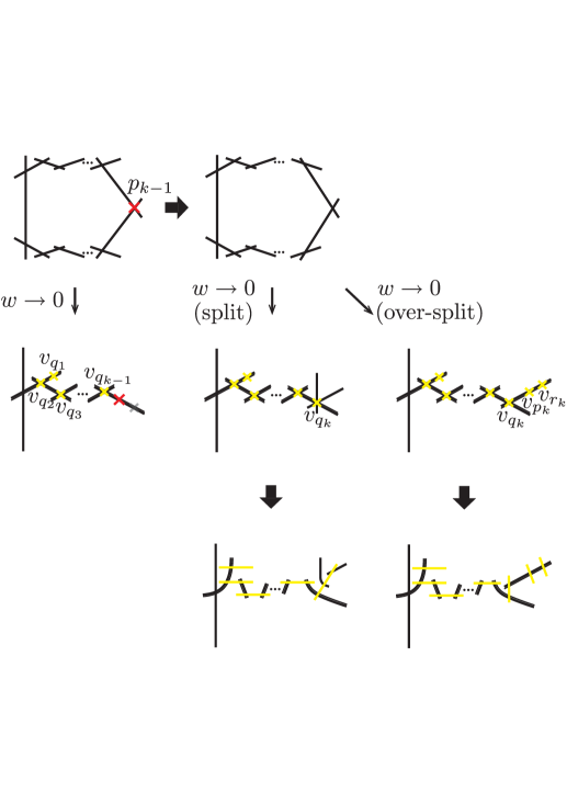
Figure 2: Singularities and exceptional curves in a split and an over-split $I_{2k+1}$ model for $k\geq 2$ near a double root of $c_{1,0}^{2}=0$.

4.1 The split, non-split and “over-split” $I_{2k+1}$ models

The vanishing orders of the sections $b_{2}$, $b_{4}$, $b_{6}$ for a $I_{2k+1}$ model are $0$, $k$, $2k$, respectively, which are the same as those for a $I_{2k}$ model. The difference from the $I_{2k}$ model is that the vanishing order of $b_{8}$ is $2k+1$ instead of $2k$, which means that

$$0=4b_{8,2k}=b_{4,k}^{2}-b_{2,0}b_{6,2k}.$$ (50)

In the split models, $b_{2,0}$ is given by a square $c_{1,0}^{2}$ for some $c_{1,0}$, so we have

$$b_{6,2k}=\left(\frac{b_{4,k}}{c_{1,0}}\right)^{2}.$$ (51)

Thus $b_{4,k}$ must be divisible by $c_{1,0}$. We can then write

$$b_{2,0} = c_{1,0}^{2},$$

$$b_{4,k} = c_{1,0}c_{3,k},$$

$$b_{6,2k} = c_{3,k}^{2}$$ (52)

for some $c_{3,k}$, which is a section of the line bundle specified by its subscripts. Again, $k=1$ is a special case so will be discussed later. For $k\geq 2$, we find

$$f = -\frac{1}{48}c_{1,0}^{4}+\cdots$$

$$\stackrel{{\scriptstyle c_{1,0}\rightarrow 0}}{{\rightarrow}} -\frac{1}{48}b_{2,1}^{2}z^{2}+\cdots,$$

$$g = \frac{1}{864}c_{1,0}^{6}+\cdots$$ (53)

$$\stackrel{{\scriptstyle c_{1,0}\rightarrow 0}}{{\rightarrow}} \frac{1}{864}b_{2,1}^{3}z^{3}+\cdots$$

and

$$\Delta = \frac{1}{16}c_{1,0}^{4}b_{8,2k+1}z^{2k+1}+\cdots$$ (54)

$$\stackrel{{\scriptstyle c_{1,0}\rightarrow 0}}{{\rightarrow}} \frac{1}{64}b_{2,1}^{3}c_{3,k}^{2}z^{2k+3}+\cdots.$$

Therefore, the zero loci of $c_{1,0}$ are where the apparent fiber type changes to $I_{2k-3}^{*}$, or from $A_{2k}$ to $D_{2k+1}$ in terms of the singularity.

In the non-split $I_{2k+1}$ models, (50) is assumed to be satisfied, but $b_{2,0}$ is not assumed to be in the form of a square. So suppose that $b_{2,0}$ is not a complete square but takes the product form

$$b_{2,0} = c_{r,0}^{2}\tilde{b}_{2-2r,0}$$ (55)

for some $c_{r,0}$ and $\tilde{b}_{2-2r,0}$. In this case, $b_{4,k}$ must be divisible by $c_{r,0}$. Then the same discussion as we did in the split $I_{2k+1}$ model can apply to show that at the zero loci of $c_{r,0}$ the fiber type changes there to $I_{2k-3}^{*}$ and the singularity is enhanced to $D_{2k+1}$.

Thus let us assume that $b_{2,0}$ is completely generic and has no square factor, that is, the equation $b_{2,0}=0$ has no double root. In this case, the constraint (50) requires that $b_{4,k}$ is divisible by $b_{2,0}$:

$$b_{2,0} :$$ generic,

$$b_{4,k} = b_{2,0}c_{2,k},$$

$$b_{6,2k} = b_{2,0}c_{2,k}^{2}$$ (56)

for some section $c_{2,k}$ of the line bundle implied by the subscripts. For $k\geq 2$, we can see that the $z$-expansions of $f$ and $g$ are similar to (53), but the discriminant in the present case is

$$\Delta = \frac{1}{16}b_{2,0}^{2}b_{8,2k+1}z^{2k+1}+\cdots$$ (57)

$$\stackrel{{\scriptstyle b_{2,0}\rightarrow 0}}{{\rightarrow}} \frac{1}{64}b_{2,1}^{2}(b_{2,1}b_{6,2k+1}-b_{4,k+1}^{2})z^{2k+4}+\cdots,$$

in which the order of $z$ at the zero loci of $b_{2,0}$ is one order higher than that in the split case. This shows that, in a non-split $I_{2k+1}$ model, the fiber type in the sense of Kodaira changes to $I_{2k-2}^{*}$ instead of $I_{2k-3}^{*}$, and the apparent singularity there is enhanced from $A_{2k}$ to $D_{2k+2}$ instead of $D_{2k+1}$.

Therefore, a generic split $I_{2k+1}$ model cannot directly transition to a non-split $I_{2k+1}$ model. The interface model that connects the split and non-split models can be obtained by tuning the complex structure of a split model so that it can yield the $D_{2k+2}$ points which are originally absent in generic split $I_{2k+1}$ models. The existence of such models was already pointed out in Tani . More specifically, we consider a special class of split $I_{2k+1}$ models in which the relevant sections $b_{2,0}$, $b_{4,k}$ and $b_{6,2k}$ are given by

$$b_{2,0} = c_{1,0}^{2}$$

$$b_{4,k} = c_{1,0}^{2}c_{2,k},$$

$$b_{6,2k} = c_{1,0}^{2}c_{2,k}^{2},$$ (58)

which we call an “over-split $I_{2k+1}$ model.” (58) can be obtained by specializing $c_{3,k}$ to the factorized form $c_{1,0}c_{2,k}$ for some $c_{2,k}$. This in particular implies that $c_{3,k}$ in (54) vanishes as $c_{1,0}\rightarrow 0$. The next non-vanishing order is $2k+4$, yielding the desired enhancement to $D_{2k+2}$. It is also clear that replacing $c_{1,0}^{2}$ with $b_{2,0}$ in (58) yields the specifications of the sections in the non-split models (56).

4.2 Conifold singularities in the $I_{2k+1}$ models for $k\geq 2$

We will now blow up the “codimension-one” singularities of the split and over-split $I_{2k+1}$ models. Since the only difference between the $I_{2k}$ and the $I_{2k+1}$ models (in their definitions) is the vanishing order of $b_{8}$, the way the singularities are blown up is very similar between the two. When we blow up the “codimension-one” singularities of a split $I_{2k+1}$ model, the first difference from the $I_{2k}$ models we encounter is the absence of the conifold singularity $v_{r_{k-1}}$ in the coordinate patch ${\mbox{\boldmath$(k-1)$}}_{\underbrace{\mbox{\scriptsize$z\cdots z$}}_{k-1}}$ (41), which appeared in the $I_{2k}$ models when $w\equiv c_{1,0}\rightarrow 0$. Instead, if we blow up the “codimension-one” singularity $p_{k-1}$, we get a pair of exceptional curves, at the intersection of which there is a conifold singularity $v_{q_{k}}$ (figure 2). If we resolve all the conifold singularities by small resolutions, we obtain the $D_{2k+1}$ Dynkin diagram as the intersection diagram of the resulting exceptional curves.

On the other hand, if we blow up the singularity $p_{k-1}$ in the over-split $I_{2k+1}$ model, the pair of exceptional lines come on top of each other to form a single irreducible line, on which three conifold singularities $v_{p_{k}},v_{q_{k}}$ and $v_{r_{k}}$ appear. Resolving all the conifold singularities gives the $D_{2k+2}$ Dynkin diagram in this case.

How these conifold singularities arise in the blowing-up process of the split and over-split $I_{2k+1}$ models near a double root of $c_{1,0}^{2}=0$ is summarized in figure 2.

4.3 The split/non-split transitions and conifold transitions in the $I_{2k+1}$ models for $k\geq 2$

Again, let us focus on a particular double root of $c_{1,0}^{2}=0$, and let it be $w=0$. Then the local equations yielding the conifold singularities $v_{q_{1}},\ldots,v_{q_{k-1}}$ are the same as those in the split $I_{2k}$ models. To see how the conifold singularities $v_{p_{k}},v_{q_{k}},v_{r_{k}}$ arise, let us consider the $k$-times blown-up equation $\Phi_{\underbrace{\mbox{\scriptsize$z\cdots z$}}_{k-1}x}(x_{k-1},y_{k},z_{k},w)=0$ in the patch ${\mbox{\boldmath$k$}}_{\underbrace{\mbox{\scriptsize$z\cdots z$}}_{k-1}x}$, where

$$\Phi_{\underbrace{\mbox{\scriptsize$z\cdots z$}}_{k-1}x}(x_{k-1},y_{k},z_{k},w) \equiv x_{k-1}^{-2}\Phi_{\underbrace{\mbox{\scriptsize$z\cdots z$}}_{k-1}}(x_{k-1},x_{k-1}y_{k},x_{k-1}z_{k},w)$$ (59)

$$= -y_{k}^{2}+x_{k-1}^{k}z_{k}^{k-1}$$

$$+{\textstyle\frac{1}{4}}(c_{1,0}^{2}+b_{2,1}x_{k-1}z_{k}+\cdots)$$

$$+{\textstyle\frac{1}{2}}(c_{1,0}c_{3,k}z_{k}+b_{4,k+1}x_{k-1}z_{k}^{2}+\cdots)$$

$$+{\textstyle\frac{1}{4}}(c_{3,k}^{2}z_{k}^{2}+b_{6,2k+1}x_{k-1}z_{k}^{3}+\cdots)$$

$$\stackrel{{\scriptstyle x_{k-1}\rightarrow 0}}{{\rightarrow}} -y_{k}^{2}+{\textstyle\frac{1}{4}}(c_{1,0}+c_{3,k}z_{k})^{2}$$

in the split case. The last line shows that the exceptional curve splits into two lines, which intersect at

$$x_{k-1}=y_{k}=c_{1,0}+c_{3,k}z_{k}=0.$$ (60)

If $c_{1,0}=0$, $z_{k}$ also vanishes for generic $c_{3,k}$; this is a conifold singularity. Indeed, we can write $\Phi_{\underbrace{\mbox{\scriptsize$z\cdots z$}}_{k-1}x}(x_{k-1},y_{k},z_{k},w)$ as, setting $c_{1,0}=w$,

$$\Phi_{\underbrace{\mbox{\scriptsize$z\cdots z$}}_{k-1}x}(x_{k-1},y_{k},z_{k},w) = -y_{k}^{2}+{\textstyle\frac{1}{4}}(w+c_{3,k}z_{k})^{2}+x_{k-1}z_{k}\left(x_{k-1}^{k-1}z_{k}^{k-2}\right.$$ (61)

$$\left.+{\textstyle\frac{1}{4}}b_{2,1}+{\textstyle\frac{1}{2}}b_{4,k+1}z_{k}+{\textstyle\frac{1}{4}}b_{6,2k+1}z_{k}^{2}+O(x_{k-1}z_{k})\right).$$

This shows that

$$v_{q_{k}}: (x_{k-1},y_{k},z_{k},w)=(0,0,0,0)~{}~{}~{}({\mbox{\boldmath$k$}}_{\underbrace{\mbox{\scriptsize$z\cdots z$}}_{k-1}x})$$ (62)

is a conifold singularity. This is the only conifold singularity in this patch in the split case. Note that the $w$-dependence of (61) is not only through $w^{2}$.

In the over-split case, (59) becomes

$$\Phi_{\underbrace{\mbox{\scriptsize$z\cdots z$}}_{k-1}x}(x_{k-1},y_{k},z_{k},w) = -y_{k}^{2}+x_{k-1}^{k}z_{k}^{k-1}$$ (63)

$$+{\textstyle\frac{1}{4}}(c_{1,0}^{2}+b_{2,1}x_{k-1}z_{k}+\cdots)$$

$$+{\textstyle\frac{1}{2}}(c_{1,0}^{2}c_{2,k}z_{k}+b_{4,k+1}x_{k-1}z_{k}^{2}+\cdots)$$

$$+{\textstyle\frac{1}{4}}(c_{1,0}^{2}c_{2,k}^{2}z_{k}^{2}+b_{6,2k+1}x_{k-1}z_{k}^{3}+\cdots)$$

$$\stackrel{{\scriptstyle x_{k-1}\rightarrow 0}}{{\rightarrow}} -y_{k}^{2}+{\textstyle\frac{1}{4}}c_{1,0}^{2}(1+c_{2,k}z_{k})^{2}.$$

Thus, the exceptional curves that are split into two lines at $c_{1,0}\neq 0$ overlap into a single line at $c_{1,0}=0$. In this case, by setting $c_{1,0}\equiv w$, (63) can be written as

$$\Phi_{\underbrace{\mbox{\scriptsize$z\cdots z$}}_{k-1}x}(x_{k-1},y_{k},z_{k},w) = -y_{k}^{2}+{\textstyle\frac{1}{4}}w^{2}(1+c_{2,k}z_{k})^{2}+x_{k-1}z_{k}\left(x_{k-1}^{k-1}z_{k}^{k-2}\right.$$ (64)

$$\left.+{\textstyle\frac{1}{4}}b_{2,1}+{\textstyle\frac{1}{2}}b_{4,k+1}z_{k}+{\textstyle\frac{1}{4}}b_{6,2k+1}z_{k}^{2}+O(x_{k-1}z_{k})\right),$$

which shows that there are three conifold singularities at $x_{k-1}=y_{k}=w=0$ and

$$z_{k}({\textstyle\frac{1}{4}}b_{2,1}+{\textstyle\frac{1}{2}}b_{4,k+1}z_{k}+{\textstyle\frac{1}{4}}b_{6,2k+1}z_{k}^{2})=0.$$ (65)

They are shown in figure 2 as $v_{q_{k}}$ (when $z_{k}=0$), $v_{p_{k}}$ and $v_{r_{k}}$ (when $z_{k}$ is one of the roots of ${\textstyle\frac{1}{4}}b_{2,1}+{\textstyle\frac{1}{2}}b_{4,k+1}z_{k}+{\textstyle\frac{1}{4}}b_{6,2k+1}z_{k}^{2}=0$). In the split case, the two points where $z_{k}$ is a non-zero root of the latter equation are not conifold singularities since the second term in (61) is $O(w^{0})$ near these points, whereas in the non-split case, the second term in (64) is $O(w^{2})$ there.

We can see that, unlike the (ordinary) split $I_{2k+1}$ case, the equation (64) is a function of $w^{2}$, so we can do the same unfolding $w^{2}\rightarrow w^{2}-\epsilon^{2}$ as we did in the $I_{2k}$ models. Again, on one hand, this replacement amounts to deforming all the conifold singularities occurring at $w=0$, and on the other hand, one of the square factors of $b_{2,0}$ becomes generic, which turns the over-split $I_{2k+1}$ model into a non-split $I_{2k+1}$ model.

4.4 The split/non-split transitions and conifold transitions in the $I_{3}$ models

Finally, to make the discussion complete, let us briefly describe the split/non-split transitions in the $I_{2k+1}$ models for $k=1$, i.e. the $I_{3}$ model. This lowest $k$ case is rather special and exhibits slightly different intersection patterns of the exceptional curves.

We have shown in figure 3 the singularities and exceptional curves in a split and an over-split $I_{3}$ model near a double root of $c_{1,0}^{2}=0$.

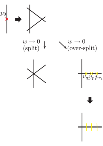
Figure 3: Singularities and exceptional curves in a split and an over-split $I_{3}$ model.

In an ordinary split $I_{3}$ model, no conifold singularity appears once the “codimension-one” singularity is blown up, even when $c_{1,0}\equiv w$ is taken to zero, where the fiber type changes from $I_{3}$ to $IV$. No matter hypermultiplet arises at the zero loci of $c_{1,0}$. In the over-split $I_{3}$ model, where we take

$$b_{2,0} = c_{1,0}^{2}$$

$$b_{4,1} = c_{1,0}^{2}c_{2,1},$$

$$b_{6,2} = c_{1,0}^{2}c_{2,1}^{2},$$ (66)

three conifold singularities appear at each zero locus of $c_{1,0}$, whose small resolutions yield exceptional curves of the $I_{0}^{*}$ type, and the singularity is enhanced from $A_{2}$ to $D_{4}$.

Although the way the conifold singularities appear is slightly different from the cases for $k\geq 2$, the over-split $I_{3}$ model is also turned into the non-split $I_{3}$ model by the replacement $w^{2}\rightarrow w^{2}-\epsilon^{2}$, which is a deformation of a conifold singularity.

5 Split/non-split transitions as conifold transitions (III): $IV$

Let us next consider the $IV$ model. The $IV$ model is defined in the Deligne form (9) for $b_{2}$, $b_{4}$, $b_{6}$ with vanishing orders $1$, $2$, $2$, respectively. The sections $f$, $g$ characterizing the Weierstrass equation read

$$f = -\frac{1}{48}(b_{2,1}^{2}-24b_{4,2})z^{2}+\cdots,$$

$$g = \frac{1}{4}b_{6,2}z^{2}+\cdots,$$

and the discriminant is

$$\Delta = \frac{27}{16}b_{6,2}^{2}z^{4}+\cdots,$$ (68)

so ord$(f,g,\Delta)=(2,2,4)$ and the generic fiber type at $z=0$ is $IV$. At the zero loci of $b_{6,2}$, they are enhanced to $(2,3,6)$, showing that the Kodaira fiber type there is $I_{0}^{*}$. If the section $b_{6,2}$ can be written in the form of a square $c_{3,1}^{2}$ for some $c_{3,1}$, the model is said a split $IV$ model, while if $b_{6,2}$ cannot be written that way, it is said a non-split $IV$ model BIKMSV .

In this case, the only “codimension-one” singularity at a generic point on $z=0$ is $p_{0}:(x,y,z,w)=(0,0,0,w)$, which can be resolved by just a one-time blow-up. The resulting exceptional curves split into two, which intersect the original fiber at a single point; they come on top of each other at $b_{6,2}=0$.

In the split case, they are all double roots, and three new conifold singularities appear on the overlapping exceptional lines. To see this, consider the equation blown up once $\Phi_{z}(x_{1},y_{1},z,w)=0$ with

$$\Phi_{z}(x_{1},y_{1},z,w) = -y_{1}^{2}+x_{1}^{3}z$$ (69)

$$+{\textstyle\frac{1}{4}}(b_{2,1}z+\cdots)x_{1}^{2}+{\textstyle\frac{1}{2}}(b_{4,2}z+\cdots)x_{1}+{\textstyle\frac{1}{4}}(w^{2}+b_{6,3}z+\cdots)$$

$$\stackrel{{\scriptstyle z\rightarrow 0}}{{\rightarrow}} -y_{1}^{2}+{\textstyle\frac{1}{4}}w^{2},$$

in ${\bf 1}_{z}$, where we have set $b_{6,2}=w^{2}$ to focus on a particular double root of $b_{6,2}=0$. (69) indeed shows that the generic exceptional curve splits into two lines, and they coincide with each other at $w=0$. Conifold singularities can be seen by rewriting (69) as

$$\Phi_{z}(x_{1},y_{1},z,w) = -y_{1}^{2}+{\textstyle\frac{1}{4}}w^{2}+z(x_{1}^{3}+{\textstyle\frac{1}{4}}b_{2,1}x_{1}^{2}+{\textstyle\frac{1}{2}}b_{4,2}x_{1}+{\textstyle\frac{1}{4}}b_{6,3}+O(z)).$$ (70)

For generic $b_{2,1}$, $b_{4,2}$, $b_{6,3}$, the cubic equation of $x_{1}$ has three distinct roots, giving rise to three conifold singularities at $y_{1}=w=z=0$. Again, the replacement $w^{2}\rightarrow w^{2}-\epsilon^{2}$ amounts to the transition from the split to non-split $IV$ model, at the same time it unfolds the conifold singularity to yield a local deformed conifold. Singularities and exceptional curves in the split $IV$ model near $w=0$ are depicted in figure 4.

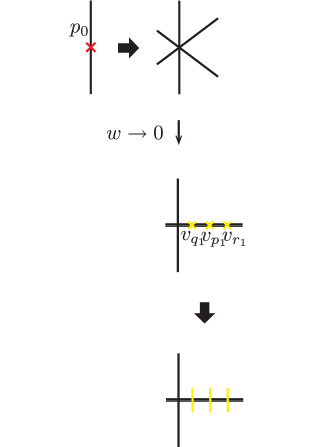
Figure 4: Singularities and exceptional curves in a split $IV$ model.

6 Split/non-split transitions as conifold transitions (IV): $IV^{*}$

In the $IV^{*}$ model, the vanishing orders of $b_{2},b_{4},b_{6}$ are $2,3,4$, respectively. $f$ and $g$ (15) are

$$f = \frac{1}{2}b_{4,3}z^{3}+\cdots,$$

$$g = \frac{1}{4}b_{6,4}z^{4}+\cdots.$$ (71)

The discriminant is

$$\Delta = \frac{27}{16}b_{6,4}^{2}z^{8}+\cdots.$$ (72)

These imply that the fiber type is $IV^{*}$ at a generic point of $z=0$. The split $IV^{*}$ model has $b_{6,4}$ in the form of a square $c_{3,2}^{2}$ for some $c_{3,2}$. The non-split $IV^{*}$ model has generic $b_{6,4}$ BIKMSV . In both the split and non-split models, the vanishing orders of $(f,g,\Delta)$ at the zero locus of $b_{6,4}$ changes from $(3,4,8)$ to $(3,5,9)$, implying that the apparent fiber type there is $III^{*}$, that is, the zero locus of $b_{6,4}$ is an $E_{7}$ point.

We have illustrated in figure 5 how the singularities appear and exceptional curves intersect in the split $IV^{*}$ model near $w=0$, which is one of the double roots of $c_{3,2}^{2}=0$. At the stage where the three “codimension-one” singularities are blown up, there remain three conifold singularities at each double root of $b_{6,4}=c_{3,2}^{2}=0$. We will show that, if all these conifold singularities are resolved by small resolutions, we obtain a smooth, fully resolved split $IV^{*}$ model, while if all the conifold singularities are simultaneously deformed, we are led to a smooth non-split $IV^{*}$ model.

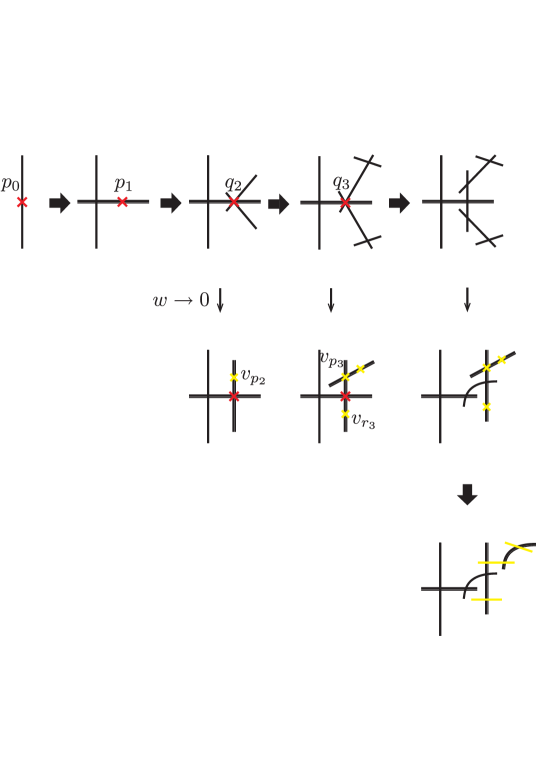
Figure 5: Singularities and exceptional curves in the split $IV^{*}$ model near a double root of $c_{3,2}^{2}=0$.

We start with a split $IV^{*}$ model. The defining equation is

$$\Phi(x,y,z,w)\equiv -y^{2}+x^{3} +{\textstyle\frac{1}{4}}b_{2,2}z^{2}x^{2}$$ (73)

$$+{\textstyle\frac{1}{2}}(b_{4,3}z^{3}+b_{4,4}z^{4})x$$

$$+{\textstyle\frac{1}{4}}(c_{3,2}^{2}z^{4}+b_{6,5}z^{5}+\cdots)=0.$$

The first “codimension-one” singularity (next to the original singularity $p_{0}$) can be found on $\Phi_{z}(x_{1},y_{1},z,w)=0$ defined in (21) with $\Phi(x,y,z,w)$ given by (73). This is

$$p_{1}: (x_{1},y_{1},z,w)=(0,0,0,0)~{}~{}~{}({\mbox{\boldmath$1$}}_{z}).$$ (74)

Blowing up $\Phi_{z}(x_{1},y_{1},z,w)=0$ at $p_{1}$, we have

$$\Phi_{zx}(x_{1},y_{2},z_{2},w)= -y_{2}^{2}+x_{1}^{2}z_{2} +{\textstyle\frac{1}{4}}b_{2,2}x_{1}^{2}z_{2}^{2}$$ (75)

$$+{\textstyle\frac{1}{2}}(b_{4,3}x_{1}z_{2}^{2}+b_{4,4}x_{1}^{2}z_{2}^{3})$$

$$+{\textstyle\frac{1}{4}}(c_{3,2}^{2}z_{2}^{2}+b_{6,5}x_{1}z_{2}^{3}+\cdots)=0,$$

where $\Phi_{zx}(x_{1},y_{2},z_{2},w)$ is defined similarly to (22). In the $x_{1}\rightarrow 0$ limit, this equation reduces to $y_{2}^{2}=0$, which is a double line. It has a “codimension-one” singularity

$$q_{2}: (x_{1},y_{2},z_{2},w)=(0,0,0,w)~{}~{}~{}({\mbox{\boldmath$2$}}_{zx})$$ (76)

as well as a conifold singularity

$$v_{p_{2}}: (x_{1},y_{2},z_{2},w)=(0,0,-\frac{2b_{4,3}}{b_{6,5}},0)~{}~{}~{}({\mbox{\boldmath$2$}}_{zx}).$$ (77)

The latter can be seen by writing (75) as

$$-y_{2}^{2}+{\textstyle\frac{1}{4}}w^{2}z_{2}^{2}+x_{1}({\textstyle\frac{1}{2}}b_{4,3}z_{2}^{2}+{\textstyle\frac{1}{4}}b_{6,5}z_{2}^{3}+O(x_{1}))=0,$$ (78)

where we again set $c_{3,2}^{2}=w^{2}$ to focus on a particular double root of $b_{6,4}=c_{3,2}^{2}=0$.

Blowing up $\Phi_{zx}(x_{1},y_{2},z_{2},w)=0$ at $q_{2}$, we have

$$\Phi_{zxx}(x_{1},y_{3},z_{3},w)= -y_{3}^{2}+x_{1}z_{3} +{\textstyle\frac{1}{4}}b_{2,2}x_{1}^{2}z_{3}^{2}$$ (79)

$$+{\textstyle\frac{1}{2}}(b_{4,3}x_{1}z_{3}^{2}+b_{4,4}x_{1}^{3}z_{3}^{3})$$

$$+{\textstyle\frac{1}{4}}(c_{3,2}^{2}z_{3}^{2}+b_{6,5}x_{1}^{2}z_{3}^{3}+\cdots)=0$$

in the patch ${\mbox{\boldmath$3$}}_{zxx}$, where we have defined

$$\Phi_{zxx}(x_{1},y_{3},z_{3},w) \equiv x_{1}^{-2}\Phi_{zx}(x_{1},x_{1}y_{3},x_{1}z_{3},w).$$ (80)

(79) still has a “codimension-one” singularity

$$q_{3}: (x_{1},y_{3},z_{3},w)=(0,0,0,w)~{}~{}~{}({\mbox{\boldmath$3$}}_{zxx}).$$ (81)

(79) has also a conifold equation, but in fact, there arise two conifold singularities after blowing up at $q_{2}$ as we displayed in figure 5, and it is only the one of two that can be seen in the patch ${\mbox{\boldmath$3$}}_{zxx}$.

To see both conifold singularities we consider

$$\Phi_{zxz}(x_{3},y_{3},z_{2},w)= -y_{3}^{2}+x_{3}^{2}z_{2} +{\textstyle\frac{1}{4}}b_{2,2}x_{3}^{2}z_{2}^{2}$$ (82)

$$+{\textstyle\frac{1}{2}}(b_{4,3}x_{3}z_{2}+b_{4,4}x_{3}^{2}z_{2}^{3})$$

$$+{\textstyle\frac{1}{4}}(c_{3,2}^{2}+b_{6,5}x_{3}z_{2}^{2}+\cdots)=0$$

in the patch ${\mbox{\boldmath$3$}}_{zxz}$, where

$$\Phi_{zxz}(x_{3},y_{3},z_{2},w) \equiv z_{2}^{-2}\Phi_{zx}(x_{3}z_{2},y_{3}z_{2},z_{2},w).$$ (83)

(82) can also be transformed into the form of a conifold equation

$$-y_{3}^{2}+{\textstyle\frac{1}{4}}w^{2}+z_{2}\left(x_{3}^{2}+{\textstyle\frac{1}{2}}b_{4,3}x_{3}+O(z_{2})\right)=0,$$ (84)

which indicates the existence of two conifold singularities

$$v_{p_{3}}: (x_{3},y_{3},z_{2},w)=(0,0,0,0),$$

$$v_{r_{3}}: (x_{3},y_{3},z_{2},w)=(-{\textstyle\frac{1}{2}}b_{4,3},0,0,0)~{}~{}~{}({\mbox{\boldmath$3$}}_{zxz}).$$ (85)

By looking at the form of the conifold equations (78) and (84) and following the discussion we have presented in the previous sections, it is now clear that the transition from the split $IV^{*}$ model to the non-split $IV^{*}$ model is the conifold transition from the resolved side to the deformed side. Note that this is the only example in which the transition occurs at an $E_{7}$ point; as we saw in the previous sections, as well as we will see in the next section, the transition always occurs at a $D_{2k}$ point in all the other examples.

7 The $I_{n}^{*}$ models

Finally, we will deal with the $I_{n}^{*}$ cases. The situation is quite different when $n$ is even and when $n$ is odd. We will consider the odd case first.

7.1 The $I_{2k-3}^{*}$ models

The $I_{2k-3}^{*}$ models $(k\geq 2)$ have a $D_{2k+1}$ singularity. In the split $I_{2k-3}^{*}$ models $(k\geq 2)$, conifold singularities appear as in the previous examples, and the deformation at the $D_{2k+2}$ points turns a split $I_{2k-3}^{*}$ model into a non-split one and can be regarded as a deformation of the conifold singularities.

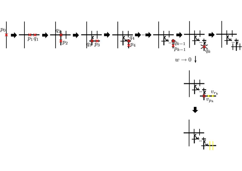
Figure 6: Singularities and exceptional curves in the split $I_{2k-3}^{*}$ model.

The model is defined by (9) with vanishing orders $\mbox{ord}(b_{2},b_{4},b_{6})=(1,k+1,2k)$ ($k\geq 2$). Whether the model is split or non-split depends on whether or not the section $b_{6,2k}$ takes the form of a square $c_{3,k}^{2}$ for some $c_{3,k}$ BIKMSV . In the split case, the Lie algebra of the unbroken gauge symmetry is $D_{2k+1}=SO(4k+2)$. Whether split or non-split, the zero loci of $b_{6,2k}$ are $D_{2k+2}=SO(4k+4)$ points. Besides them, $E_{6}$ and $E_{8}$ points may occur for $k=2$ and $3$, but they are not important here.

As we have shown in figure 6, one of the differences in the split $I_{n}^{*}$ model is that the conifold singularities appear only at the final step of blowing up. We can see the conifold singularities in the equation $\Phi_{\underbrace{\mbox{\scriptsize$z\cdots z$}}_{k}}(x_{k},y_{k},z,w)=0$, where, setting $c_{3,k}^{2}\equiv w^{2}$,

$$\Phi_{\underbrace{\mbox{\scriptsize$z\cdots z$}}_{k}}(x_{k},y_{k},z,w)= -y_{k}^{2}+x_{k}^{3}z^{k} +{\textstyle\frac{1}{4}}(b_{2,1}z+\cdots)x_{k}^{2}$$

$$+{\textstyle\frac{1}{2}}(b_{4,k+1}z+\cdots)x_{k}$$

$$+{\textstyle\frac{1}{4}}(w^{2}+b_{6,2k+1}z+\cdots)$$

$$= -y_{k}^{2}+{\textstyle\frac{1}{4}}w^{2} +z\left({\textstyle\frac{1}{4}}b_{2,1}x_{k}^{2}+{\textstyle\frac{1}{2}}b_{4,k+1}x_{k}+{\textstyle\frac{1}{4}}b_{6,2k+1}+O(z)\right).$$ (86)

The discriminant of the quadratic equation ${\textstyle\frac{1}{4}}b_{2,1}x_{k}^{2}+{\textstyle\frac{1}{2}}b_{4,k+1}x_{k}+{\textstyle\frac{1}{4}}b_{6,2k+1}=0$ is proportional to $b_{8,2k+2}$, which does not vanish generically. Therefore it has two distinct roots, yielding the two conifold singularities. The equation (86) again depends on $w$ through $w^{2}$ near the singularities, and unfolding the conifold singularity is exactly what turns a split model into a non-split one.

7.2 The $I_{2k-2}^{*}$ models

So far we have seen various examples in which the split/non-split transition is precisely the conifold transition associated with the conifold singularities occurring at the $D_{2k}$ points, or the $E_{7}$ points in the $IV^{*}$ case. In fact, in the $I_{2k-2}^{*}$ model, the situation is quite different. The crucial difference is that, in that case, no conifold singularity arises at the zero locus of the section relevant to the split/non-split transition.

In this class of models, the orders of $b_{2}$, $b_{4}$, $b_{6}$ are $1$, $k+1$, $2k+1$, instead of $1$, $k+1$, $2k$ in the previous $I_{2k-3}^{*}$ models. $k=1$ is a special case and has already been discussed in detail in EsoleetalSO(8) , so we will consider $k\geq 2$. $f$ and $g$ (15) read

$$f = -\frac{1}{48}b_{2,1}^{2}z^{2}+\cdots,$$

$$g = +\frac{1}{864}b_{2,1}^{3}z^{3}+\cdots,$$ (87)

which are the same as those in the $I_{2k-3}^{*}$ models. The discriminant is

$$\Delta = \frac{1}{16}b_{2,1}^{2}b_{8,2k+2}z^{2k+4}+\cdots,$$ (88)

so, for a generic $b_{2,1}$, the singularity is enhanced from $D_{2k+2}$ to $D_{2k+3}$ at the zero locus of $b_{8,2k+2}$, where

$$b_{8,2k+2} = \frac{1}{4}(b_{2,1}b_{6,2k+1}-b_{4,k+1}^{2}).$$ (89)

If this $b_{8,2k+2}$ is written as $c_{4,k+1}^{2}$ for some $c_{4,k+1}$, this $I_{2k-2}^{*}$ model is called split, otherwise non-split BIKMSV .

The blowing-up procedure proceeds similarly to the $I_{2k-3}^{*}$ models. In the split case, a difference arises when $p_{k-1}$ is blown up, where the exceptional curves overlap to one line instead of splitting into two lines, and three “codimension-one” singularities arise on the line. This is precisely what was seen in the $w\rightarrow 0$ limit after $p_{k-1}$ was blown up in the $I_{2k-3}^{*}$ models, where the two conifold singularities found there are now replaced by two “codimension-one” singularities (figure 7).

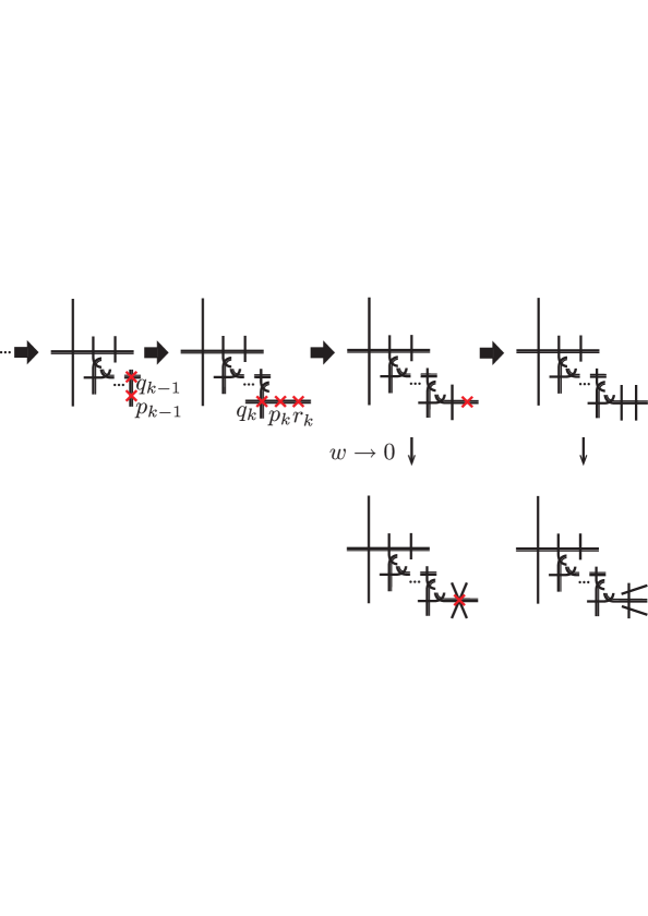
Figure 7: Singularities and exceptional curves in the split $I_{2k-2}^{*}$ model.

Concretely,

$$\Phi_{\underbrace{\mbox{\scriptsize$z\cdots z$}}_{k}}(x_{k},y_{k},z,w)= -y_{k}^{2}+x_{k}^{3}z^{k} +{\textstyle\frac{1}{4}}(b_{2,1}z+\cdots)x_{k}^{2}$$ (90)

$$+{\textstyle\frac{1}{2}}(b_{4,k+1}z+\cdots)x_{k}$$

$$+{\textstyle\frac{1}{4}}(b_{6,2k+1}z+\cdots).$$

Since $b_{8,2k+2}$ is proportional to the discriminant of the quadratic equation of ${\textstyle\frac{1}{4}}b_{2,1}x_{k}^{2}+{\textstyle\frac{1}{2}}b_{4,k+1}x_{k}+{\textstyle\frac{1}{4}}b_{6,2k+1}=0$, we can further write, by assuming $b_{8,2k+2}=c_{4,k+1}^{2}$, as

$$\Phi_{\underbrace{\mbox{\scriptsize$z\cdots z$}}_{k}}(x_{k},y_{k},z,w) = -y_{k}^{2}+z\left({\textstyle\frac{1}{4}}b_{2,1}x_{k}^{2}+{\textstyle\frac{1}{2}}b_{4,k+1}x_{k}+{\textstyle\frac{1}{4}}b_{6,2k+1}+O(z)\right)$$ (91)

$$= -y_{k}^{2}+\frac{z}{b_{2,1}}\left(\left(\frac{b_{2,1}}{2}x_{k}+b_{4,k+1}\right)^{2}+c_{4,k+1}^{2}+O(z)\right).$$

Thus, the “codimension-one” singular loci of $\Phi_{\underbrace{\mbox{\scriptsize$z\cdots z$}}_{k}}(x_{k},y_{k},z,w)=0$ split into two irreducible components

$$y_{k}=0,~{}z=0,~{}\frac{b_{2,1}}{2}x_{k}+b_{4,k+1}\pm ic_{4,k+1}=0.$$ (92)

Their intersection is where $c_{4,k+1}$ vanishes, or equivalently, $b_{8,2k+2}=0$ vanishes, so it is a $D_{2k+3}$ point. The “codimension-one” singularities can be blown up along either of the two irreducible components (92) first. One can verify that the exceptional curve obtained in such a way splits into two lines precisely at the intersection $D_{2k+3}$ point. Blowing up along the remaining irreducible component thus yields the $D_{2k+3}$ intersection diagram only there. This is how the higher-rank intersection diagram emerges without conifold singularities in the $I_{2k-2}^{*}$ models.

On the other hand, the equation of the non-split $I_{2k-2}^{*}$ model can be obtained by replacing $c_{4,k+1}^{2}$ with a generic $b_{8,2k+2}$ in (91). In this case, the “codimension-one” singular loci consist of only one irreducible component, along which we can blow up the singularities only once. No conifold singularity is found. Therefore, only the $I_{2k-2}^{*}$ models (including the $I_{0}^{*}$ model EsoleetalSO(8) ) cannot interpret the split/non-split transition there as a conifold transition.

8 Conclusions

In this paper, we have shown that in six-dimensional F-theory on elliptic Calabi-Yau threefolds on the Hirzebruch surface $\hbox{\mybb F}_{n}$, all the non-split models listed in BIKMSV , except a certain class of fiber types, can be realized by a conifold transition from the corresponding split models. We examined this fact separately for all cases of $I_{n}$ ($n\geq 3$), $I_{n}^{*}$ ($n\geq 0$), $IV$ and $IV^{*}$, in which there is a distinction between the split and non-split types.

In the split models of the fiber types $I_{2k}$ ($k\geq 2$), $IV$ and $I_{2k-3}^{*}$ ($k\geq 2$), there generically exist points where the singularities $SU(2k)$, $SU(3)$ and $SO(4k+2)$ are enhanced to $SO(4k)$, $SO(8)$ and $SO(4k+4)$ in the sense of Kodaira. When all the “codimension-one” singularities are blown up, there remain some conifold singularities there. If these conifold singularities are resolved by small resolutions, one obtains a smooth split model for each case. This is the resolved side of the conifold transition. On the other hand, at the stage where all the “codimension-one” singularities are blown up, one can also deform the relevant section so that the split model transforms into the non-split model, thereby all the conifold singularities are simultaneously unfolded. This is the deformed side of the conifold transition.

The $IV^{*}$ model is similar to these models, but only in this case, the singularity of the enhanced point where the conifold transition occurs is $E_{7}$ instead of $SO(4k)$.

The split $I_{2k-1}$ model has generically an $SU(2k-1)$ singularity and has no $SO(4k)$ point in general. However, by adjusting the complex structure, one can make the $SO(4k-2)$ point and the $SU(2k)$ point come to the same point to achieve an $SO(4k)$ point. We called such a split $I_{2k-1}$ model with a special complex structure an “over-split” model. We found that in this case, there arose conifold singularities at the $SO(4k)=D_{2k}$ point after blowing up all the “codimension-one” singularities. Then the non-split $I_{2k-1}$ model is obtained by the deformation similarly.

Finally, in the case of the $I_{2k-2}^{*}$ models, the conifold singularity does not appear after the blow-up of the “codimension-one” singularities. Therefore, this is a special case in which the split/non-split transition cannot be regarded as a conifold transition.

We have also examined how the proposal of AKM for the origin of non-local matter can be actually implemented in our blow-up analysis. We have shown that the genus-$g$ Riemann surface that plays the essential role in the proposal can be obtained as an intersection of the blown-up three-fold and an appropriate divisor, and by forgetting the $\hbox{\mybb P}^{1}$ fiber direction. It has also been found that even when there are multiple pairs of exceptional curves, the genus-$g$ Riemann surface obtained from them are all identical and thus well-defined.

Conifold singularities are ubiquitous, associated with matter generations in F-theory. As we stressed, these are not the ones created by some fine tuning of moduli, but always occur where matter is generated in the very general setting in F-theory. The conifold transition has been an important key concept in discussions in AdS/CFT KW ; KS , topological string theory GV ; VafalargeN , and string cosmology (e.g. GKP ; KKLT ). In view of these facts, it would be very interesting to consider new applications of the facts revealed here to the theory of superstring phenomenology and cosmology.

- (1) C. Vafa, Evidence for F theory, Nucl. Phys. B 469, 403 (1996), arXiv: hep-th/9602022.
- (2) D. R. Morrison and C. Vafa, Compactifications of F theory on Calabi-Yau threefolds. 1, Nucl. Phys. B 473, 74 (1996), arXiv: hep-th/9602114.
- (3) D. R. Morrison and C. Vafa, Compactifications of F theory on Calabi-Yau threefolds. 2., Nucl. Phys. B 476, 437 (1996), arXiv: hep-th/9603161.
- (4) M. Bershadsky, K. Intriligator, S. Kachru, D.R. Morrison, V. Sadov and C. Vafa, Geometric singularities and enhanced gauge symmetries, Nucl.Phys. B481 (1996) 215-252, arXiv: hep-th/9605200.
- (5) S. H. Katz and C. Vafa, Matter from geometry, Nucl. Phys. B 497, 146 (1997), arXiv: hep-th/9606086.
- (6) K. Kodaira, Ann. of Math. 77, 563 (1963).
- (7) R. Donagi and M. Wijnholt, Model Building with F-Theory, Adv. Theor. Math. Phys. 15, 1237 (2011), arXiv:0802.2969 [hep-th].
- (8) C. Beasley, J. J. Heckman and C. Vafa, GUTs and Exceptionl Branes in F-theory - I, JHEP 0901, 058 (2009), arXiv:0802.3391 [hep-th].
- (9) C. Beasley, J. J. Heckman and C. Vafa, GUTs and Exceptional Branes in F-theory - II: Experimental Predictions, JHEP 0901, 059 (2009), arXiv:0806.0102 [hep-th].
- (10) R. Donagi and M. Wijnholt, Breaking GUT Groups in F-Theory, Adv. Theor. Math. Phys. 15, 1523 (2011), arXiv:0808.2223 [hep-th].
- (11) H. Hayashi, T. Kawano, R. Tatar and T. Watari, Codimension-3 Singularities and Yukawa Couplings in F-theory, Nucl. Phys. B 823 (2009) 47 ,arXiv:0901.4941 [hep-th].
- (12) R. Donagi and M. Wijnholt, Higgs Bundles and UV Completion in F-Theory, Commun. Math. Phys. 326 (2014) 287 ,arXiv:0904.1218 [hep-th].
- (13) J. J. Heckman, J. Marsano, N. Saulina, S. Schafer-Nameki and C. Vafa, Instantons and SUSY breaking in F-theory, arXiv:0808.1286 [hep-th].
- (14) J. Marsano, N. Saulina and S. Schafer-Nameki, Gauge Mediation in F-Theory GUT Models, Phys. Rev. D 80 (2009) 046006 , arXiv:0808.1571 [hep-th].
- (15) J. J. Heckman and C. Vafa, F-theory, GUTs, and the Weak Scale, JHEP 0909 (2009) 079 , arXiv:0809.1098 [hep-th].
- (16) A. Font and L. E. Ibanez, Yukawa Structure from U(1) Fluxes in F-theory Grand Unification, JHEP 0902 (2009) 016 , arXiv:0811.2157 [hep-th].
- (17) D. R. Morrison and W. Taylor, Matter and singularities, JHEP 1201, 022 (2012), arXiv:1106.3563 [hep-th].
- (18) M. Esole and S. T. Yau, Small resolutions of SU(5)-models in F-theory, Adv. Theor. Math. Phys. 17, no. 6, 1195 (2013), arXiv:1107.0733 [hep-th].
- (19) D. R. Morrison and W. Taylor, Classifying bases for 6D F-theory models, Central Eur. J. Phys. 10 (2012), 1072-1088 [arXiv:1201.1943 [hep-th]].
- (20) M. B. Green, J. H. Schwarz and P. C. West, Anomaly Free Chiral Theories in Six-Dimensions, Nucl. Phys. B 254, 327 (1985).
- (21) A. Grassi, J. Halverson, C. Long, J. L. Shaneson and J. Tian, Non-simply-laced Symmetry Algebras in F-theory on Singular Spaces,, JHEP 09 (2018), 129 , arXiv:1805.06949 [hep-th].
- (22) P. Arras, A. Grassi and T. Weigand, Terminal Singularities, Milnor Numbers, and Matter in F-theory, J. Geom. Phys. 123 (2018), 71-97, arXiv:1612.05646 [hep-th].
- (23) M. Esole, P. Jefferson and M. J. Kang, The Geometry of F4-Models, arXiv:1704.08251 [hep-th].
- (24) M. Esole and M. J. Kang, The Geometry of the SU(2) G2-model, JHEP 02 (2019), 091, arXiv:1805.03214 [hep-th].
- (25) M. Esole and P. Jefferson, USp(4)-models, arXiv:1910.09536 [hep-th].
- (26) N. Kan, S. Mizoguchi and T. Tani, Half-hypermultiplets and incomplete/complete resolutions in F-theory, JHEP 08, 063 (2020) , arXiv:2003.05563 [hep-th].
- (27) R. Kuramochi, S. Mizoguchi and T. Tani, Magic square and half-hypermultiplets in F-theory, arXiv:2008.09272 [hep-th].
- (28) J. Marsano and S. Schafer-Nameki, Yukawas, G-flux, and Spectral Covers from Resolved Calabi-Yau’s, JHEP 1111, 098 (2011) , arXiv:1108.1794 [hep-th].
- (29) H. Hayashi, C. Lawrie, D. R. Morrison and S. Schafer-Nameki, Box Graphs and Singular Fibers, JHEP 05, 048 (2014) [arXiv:1402.2653 [hep-th]].
- (30) P. S. Aspinwall, S. H. Katz and D. R. Morrison, Lie groups, Calabi-Yau threefolds, and F theory, Adv. Theor. Math. Phys. 4, 95-126 (2000), arXiv:hep-th/0002012 [hep-th].
- (31) P. Candelas, X. de la Ossa. P. Green and L. Parkes, A Pair of Calabi-Yau Manifolds as an Exactly Soluble Superconformal Field Theory, Nucl. Phys. B359 (1991) 21.
- (32) P. Candelas, P. Green and T. Hubsch, Rolling Among Calabi-Yau Vacua, Nucl. Phys. B330 (1990) 49.
- (33) P. Candelas and X. de la Ossa, Comments on Conifolds, Nucl. Phys. B342 (1990) 246.
- (34) P. Candelas and X. de la Ossa, Moduli Space of Calabi-Yau Manifolds, Nucl. Phys. B355 (1991) 455.
- (35) P. Aspinwall, B. Greene and D. Morrison, B416 (1994) 414.
- (36) A. Strominger, Massless black holes and conifolds in string theory, Nucl. Phys. B 451, 96-108 (1995) , arXiv:hep-th/9504090 [hep-th].
- (37) A. Grassi, J. Halverson and J. L. Shaneson, Matter From Geometry Without Resolution, JHEP 1310, 205 (2013) , arXiv:1306.1832 [hep-th].
- (38) A. Grassi, J. Halverson and J. L. Shaneson, Non-Abelian Gauge Symmetry and the Higgs Mechanism in F-theory, Commun. Math. Phys. 336, no.3, 1231-1257 (2015) , arXiv:1402.5962 [hep-th].
- (39) S. B. Giddings, S. Kachru and J. Polchinski, Hierarchies from fluxes in string compactifications, Phys. Rev. D 66, 106006 (2002) , arXiv:hep-th/0105097 [hep-th].
- (40) K. Intriligator, H. Jockers, P. Mayr, D. R. Morrison and M. R. Plesser, Conifold Transitions in M-theory on Calabi-Yau Fourfolds with Background Fluxes, Adv. Theor. Math. Phys. 17, no.3, 601-699 (2013) , arXiv:1203.6662 [hep-th].
- (41) P. S. Aspinwall, M theory versus F theory pictures of the heterotic string, Adv. Theor. Math. Phys. 1, 127-147 (1998) , arXiv:hep-th/9707014 [hep-th].
- (42) P. Deligne, Lecture Notes in Math., Vol. 476, Springer, Berlin, 1975.
- (43) M. Esole, R. Jagadeesan and M. J. Kang, The Geometry of G2, Spin(7), and Spin(8)-models, arXiv:1709.04913 [hep-th].
- (44) S. Katz, D. R. Morrison, S. Schafer-Nameki and J. Sully, Tate’s algorithm and F-theory, JHEP 08, 094 (2011) , arXiv:1106.3854 [hep-th].
- (45) C. Lawrie and S. Schäfer-Nameki, The Tate Form on Steroids: Resolution and Higher Codimension Fibers, JHEP 04, 061 (2013) [arXiv:1212.2949 [hep-th]].
- (46) S. Mizoguchi and T. Tani, Looijenga’s weighted projective space, Tate’s algorithm and Mordell-Weil Lattice in F-theory and heterotic string theory, JHEP 11, 053 (2016) , arXiv:1607.07280 [hep-th].
- (47) L. B. Anderson, J. Gray, N. Raghuram and W. Taylor, Matter in transition, JHEP 04, 080 (2016) , arXiv:1512.05791 [hep-th].
- (48) V. Sadov, Generalized Green-Schwarz mechanism in F theory, Phys. Lett. B 388, 45 (1996) [hep-th/9606008].
- (49) E. Witten, Phase transitions in M theory and F theory, Nucl. Phys. B 471 (1996), 195-216 [arXiv:hep-th/9603150 [hep-th]].
- (50) S. H. Katz, D. R. Morrison and M. R. Plesser, Enhanced gauge symmetry in type II string theory, Nucl. Phys. B 477 (1996), 105-140 [arXiv:hep-th/9601108 [hep-th]].
- (51) S. Mizoguchi and T. Tani, Non-Cartan Mordell-Weil lattices of rational elliptic surfaces and heterotic/F-theory compactifications, JHEP 03, 121 (2019) , arXiv:1808.08001 [hep-th].
- (52) T. Tani, Matter from string junction, Nucl. Phys. B 602, 434 (2001).
- (53) I. R. Klebanov and E. Witten, Superconformal field theory on three-branes at a Calabi-Yau singularity, Nucl. Phys. B 536, 199-218 (1998) , arXiv:hep-th/9807080 [hep-th].
- (54) I. R. Klebanov and M. J. Strassler, Supergravity and a confining gauge theory: Duality cascades and chi SB resolution of naked singularities, JHEP 08, 052 (2000) , arXiv:hep-th/0007191 [hep-th].
- (55) R. Gopakumar and C. Vafa, On the gauge theory / geometry correspondence, Adv. Theor. Math. Phys. 3, 1415-1443 (1999) , arXiv:hep-th/9811131 [hep-th].
- (56) C. Vafa, Superstrings and topological strings at large N, J. Math. Phys. 42, 2798-2817 (2001), arXiv:hep-th/0008142 [hep-th].
- (57) S. Kachru, R. Kallosh, A. D. Linde and S. P. Trivedi, De Sitter vacua in string theory, Phys. Rev. D 68, 046005 (2003), arXiv:hep-th/0301240 [hep-th].