Recurrent Video Deblurring with Blur-Invariant Motion Estimation and Pixel Volumes

Abstract.

For the success of video deblurring, it is essential to utilize information from neighboring frames. Most state-of-the-art video deblurring methods adopt motion compensation between video frames to aggregate information from multiple frames that can help deblur a target frame. However, the motion compensation methods adopted by previous deblurring methods are not blur-invariant, and consequently, their accuracy is limited for blurry frames with different blur amounts. To alleviate this problem, we propose two novel approaches to deblur videos by effectively aggregating information from multiple video frames. First, we present blur-invariant motion estimation learning to improve motion estimation accuracy between blurry frames. Second, for motion compensation, instead of aligning frames by warping with estimated motions, we use a pixel volume that contains candidate sharp pixels to resolve motion estimation errors. We combine these two processes to propose an effective recurrent video deblurring network that fully exploits deblurred previous frames. Experiments show that our method achieves the state-of-the-art performance both quantitatively and qualitatively compared to recent methods that use deep learning.

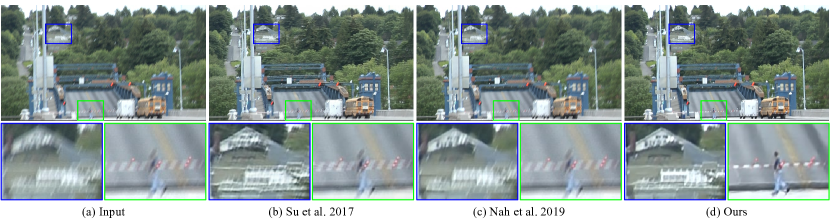
Figure 1. Deblurring results of a real-world video frame with large blur. Our method successfully restores the challenging video frame compared to other state-of-the-art methods. The input video frame is from Su et al. (2017)’s test set.

1. Introduction

Videos captured by hand-held devices are vulnerable to motion blur due to camera shakes and object motion. Video deblurring increases the visual quality of a video, and can also improve the accuracy of other video processing tasks, such as object recognition (Kupyn et al., 2018), tracking (Seibold et al., 2017), and 3D reconstruction (Lee and Lee, 2013). Numerous video deblurring methods have been proposed, including deconvolution-based (Kim and Lee, 2015; Ren et al., 2017), aggregation-based (Cho et al., 2012; Delbracio and Sapiro, 2015b), and deep learning-based approaches (Su et al., 2017; Kim et al., 2017, 2018; Nah et al., 2019; Wang et al., 2019).

Video deblurring methods typically rely on information about motion between neighboring frames, because it can be used for roughly estimating the blur and aligning frames to provide different captures of the same scene. Deconvolution-based methods (Kim and Lee, 2015; Ren et al., 2017) exploit motion between neighboring frames to estimate spatially-varying blur kernels, which are then used to deconvolve blurry frames and restore sharp frames. Aggregation-based methods (Cho et al., 2012; Delbracio and Sapiro, 2015b) use motion information to directly aggregate sharp pixels from neighboring frames. Recent deep learning-based methods (Su et al., 2017; Kim et al., 2017, 2018; Nah et al., 2019; Wang et al., 2019) train deep convolutional neural networks (CNNs) to directly produce deblurred frames from multiple input frames. While some deep learning-based methods do not explicitly assume aligned input frames, Su et al. (2017) show that rough alignment can increase deblurring quality.

However, accurate estimation of motion is challenging in the presence of blur, and incorrectly estimated motion may cause structural deformations during the motion compensation process, and thereby eventually degrade the deblurring quality. To resolve this problem, we introduce two novel approaches: blur-invariant motion estimation learning and pixel volume-based motion compensation. First, to estimate motion accurately, we adopt LiteFlowNet (Hui et al., 2018) and train it with a blur-invariant loss so that the trained network can estimate blur-invariant optical flow between frames. We refer the resulting network as a blur-invariant motion estimation network (BIMNet). Second, for effective motion compensation, instead of aligning a frame by warping, we construct a pixel volume that consists of multiple matching candidates for each pixel. Compared to a warped frame, our pixel volume provides additional information for a deblurring network to robustly restore a sharp frame, even under slight motion estimation errors.

By leveraging pixel volume-based motion compensation with blur-invariant motion estimation, we propose an effective video deblurring framework that is based on a recurrent CNN structure. To produce a deblurred result of the current frame, our framework takes four video frames as input: the previous, current, and next blurry input frames, and the deblurred result of the previous frame. In this way, we can exploit restored information of the previous frame as well as other information in neighboring input frames. Our framework then estimates motion between the current and previous frames in a blur-invariant way by using BIMNet, then uses the estimated motion to construct a pixel volume from the deblurred previous frame. Finally, our deblurring network restores a sharp image for the current frame using the pixel volume with input blurry frames.

We refer to our deblurring network as a pixel volume-based deblurring network (PVDNet). Due to BIMNet and pixel volume, PVDNet can produce visually pleasing deblurring results (Fig. 1). Experimental results show that our framework achieves the state-of-the-art performance both quantitatively and qualitatively.

Our main contributions are summarized as follows.

• We present blur-invariant learning of a motion estimation network for blurry video frames, which is essential for accurate alignment of neighboring frames.

• We propose a novel pixel volume of matching candidates for motion compensation, which provides additional information for robust reconstruction of sharp frames.

• We propose an effective recurrent CNN framework based on BIMNet and pixel volume for video deblurring.

2. Related Work

2.1. Video deblurring

Deconvolution-based approaches

Typical single image deblurring approaches (Cho and Lee, 2009; Xu and Jia, 2010; Hirsch et al., 2011; Whyte et al., 2012; Kim et al., 2013; Pan et al., 2016; Xu and Jia, 2012) estimate blur kernels and restore latent sharp images by applying deconvolution with the estimated kernels. However, estimating spatially-varying blur, which is common in the real world, is a severely ill-posed problem. Therefore, many approaches assume specific blur models and focus on limited cases such as camera shakes (Hirsch et al., 2011; Whyte et al., 2012), moving objects (Kim et al., 2013; Pan et al., 2016) and depth variation (Xu and Jia, 2012).

Video deblurring based on deconvolution also requires estimation of spatially-varying blur kernels. Early approaches (Bar et al., 2007; Wulff and Black, 2014) used segmentation maps to reduce the ill-posedness and to effectively process blur caused by moving objects. Later methods (Kim and Lee, 2015; Ren et al., 2017) proposed video deblurring frameworks based on optical flow to model inter-frame motion. These methods alternatingly perform optical flow estimation and image deblurring. However, they still assume relatively simple blur models, so can fail when applied to real-world videos that include complex blur.

Multi-frame aggregation-based approaches

A few methods (Matsushita et al., 2006; Cho et al., 2012; Delbracio and Sapiro, 2015b) assume that input frames are differently blurred, and have different partial information about latent sharp frames. Then, by aggregating such partial information on the current frame, deblurring can be done without deconvolution. These methods are usually performed in combination with frame alignment. Matsushita et al. (2006) align video frames by using a homography, then blend them to remove blur. Cho et al. (2012) introduced patch-based local search to increase the accuracy of pixel-wise correspondence between video frames. The patch-based local search yields visually pleasing results by directly blending sharp patches from neighboring frames. To achieve video deblurring, Delbracio and Sapiro (2015b) combined a multi-frame deblurring method for burst shot (Delbracio and Sapiro, 2015a) with optical flow-based frame alignment. As these methods do not use deconvolution, they could be computationally more efficient and produce less artifacts. However, they cannot restore sharp frames when all input frames are blurry.

Deep learning-based approaches

Several approaches use neural networks that are trained to automatically aggregate information from neighboring frames and reconstruct deblurred frames. Su et al. (2017) proposed a CNN that receives multiple frames concatenated together as input. They also showed rough motion compensation between input frames helps to deblur difficult scenes with large motions. Kim et al. (2017) and Nah et al. (2019) presented recurrent CNNs for video deblurring, and showed that utilizing previous results can improve deblurring quality. However, these methods do not work well for videos with large motion, as they do not use motion compensation. Recently, a spatio-temporal transformer network (Kim et al., 2018) was proposed to improve motion compensation performance for video restoration tasks, such as video super-resolution and video deblurring. The network estimates optical flow from multiple neighboring frames together to effectively handle occlusions. More recently, Wang et al. (2019) proposed an alignment module based on deformable convolutions for video restoration tasks that allows more effective utilization of information from other video frames.

2.2. Blur-invariant optical flow

There have been a small number of approaches to computing optical flow between frames with spatially-varying blurs, such as Portz et al. (2012) and Daraei (2014). To take account of blur in the searching process, both methods blur each input frame with the blur kernel of the other frame. While they can increase the accuracy of the estimation of optical flow, they are computationally heavy because of iterative update of optical flow and blur kernels. Furthermore, they use simple parametric blur models that combine two linear motions by considering forward and backward optical flows, and therefore do not generalize well to real-world blurry videos.

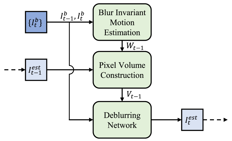
Figure 2. Our video deblurring framework.

3. Our Video Deblurring Framework

Our video deblurring framework consists of three modules: a blur-invariant motion estimation network (BIMNet), a pixel volume generator, and a pixel volume-based deblurring network (PVDNet) (see Fig. 2). We first train BIMNet; after it has converged, we combine the two networks with the pixel volume generator. We then fix the parameters of BIMNet and train PVDNet by training the entire network.

The framework takes three consecutive input blurry frames $I_{t-1}^{b}$, $I_{t}^{b}$, and $I_{t+1}^{b}$, and the deblurred result of the previous frame $I_{t-1}^{est}$ as input where $I_{t}^{b}$ is the $t$-th input blurry frame. Our BIMNet first estimates optical flow $W_{t-1}$ from $I_{t}^{b}$ to $I_{t-1}^{b}$ (Sec. 3.1). The pixel volume generator then takes $W_{t-1}$ and $I_{t-1}^{est}$, and constructs a pixel volume by using pixel values of $I_{t-1}^{est}$ according to $W_{t-1}$ (Sec. 3.2). Finally, our PVDNet takes the pixel volume $V_{t-1}$ and the input blurry frames $\{I_{t-1}^{b},I_{t}^{b},I_{t+1}^{b}\}$, and produces a deblurring result $I_{t}^{est}$ for the current frame $I_{t}^{b}$ (Sec. 3.3).

We feed a pixel volume $V_{t-1}$ obtained from the restored frame $I_{t-1}^{est}$ into PVDNet, then the use of $I_{t-1}^{b}$ as input of PVDNet may seem unnecessary. However, $I_{t-1}^{b}$ is occasionally sharper than $I_{t-1}^{est}$ especially when camera motion is not significant, and PVDNet can take advantage of $I_{t-1}^{b}$ in such cases. In addition, we apply motion compensation not to $I_{t-1}^{b}$ and $I_{t+1}^{b}$ but only to $I_{t-1}^{est}$. This choice may seem counterintuitive, but preliminary experiments demonstrated that it maximizes the deblurring performance of PVDNet (Appendix B.2).

3.1. Blur-invariant motion estimation learning

Our BIMNet adopts the network architecture of LiteFlowNet (Hui et al., 2018), which takes two images and generates optical flow between them. FlowNet (Dosovitskiy et al., 2015) and its follow-up works, FlowNet2 (Ilg et al., 2017) and LiteFlowNet (Hui et al., 2018), have a Siamese network structure for the encoder, and we found that the structure enables effective blur-invariant feature learning (Appendix A.1). We adopt LiteFlowNet for the network structure of BIMNet, because LiteFlowNet shows comparable accuracy to FlowNet2 with far fewer parameters (Sec. 4.2). Originally, LiteFlowNet was trained using blur-free datasets that provide ground truth optical flow maps, such as Scene Flow (Mayer et al., 2016), Sintel (Butler et al., 2012), KITTI (Geiger et al., 2012), and Middlebury (Scharstein et al., 2014). However, no available dataset has ground truth optical flow maps for blurry images. Thus, we train our BIMNet in a self-supervised way by using a blurred video dataset (Su et al., 2017) that contains pairs of sharp and blurred videos.

A successfully trained BIMNet should be able to produce accurate optical flow from a pair of video frames regardless of the amounts of blur that the frames include. To train the network to acquire this property, we generate four pairs of frames from each pair of consecutive frames in sharp and blurred videos: $(I_{t-1}^{s},I_{t}^{s})$, $(I_{t-1}^{b},I_{t}^{b})$, $(I_{t-1}^{b},I_{t}^{s})$, and $(I_{t-1}^{s},I_{t}^{b})$, where $I_{t}^{s}$ and $I_{t}^{b}$ are the $t$-th frames in sharp and blurred videos, respectively. For each image pair $(I_{t-1}^{\alpha},I_{t}^{\beta})$, where $\alpha,\beta\in\{s,b\}$, our BIMNet estimates optical flow $W^{\alpha\beta}_{t}$ from $I_{t}^{\beta}$ to $I_{t-1}^{\alpha}$.

Then, we train BIMNet with a blur-invariant loss $L_{BIM}^{\alpha\beta}$ for every pair ($\alpha$, $\beta$):

(1) $$L_{BIM}^{\alpha\beta}=MSE(Warp(I_{t-1}^{s},W^{\alpha\beta}_{t}),I_{t}^{s}),$$

where $MSE$ computes the mean squared error between two images and $Warp(I_{t-1}^{s},W^{\alpha\beta}_{t})$ is a warping of $I_{t-1}^{s}$ by $W^{\alpha\beta}_{t}$. $Warp$ can be easily implemented using the sampling layer of the spatial transformer network (Jaderberg et al., 2015). The key idea of $L_{BIM}^{\alpha\beta}$ is that it induces BIMNet to learn optical flow between sharp frames, $I_{t-1}^{s}$ and $I_{t}^{s}$, as the ground truth regardless of the blur types of input images, $I_{t-1}^{\alpha}$ and $I_{t}^{\beta}$.

A straightforward idea for blur-invariant learning would be to estimate optical flow maps between sharp video frames and use them as ground truth labels for training optical flow estimation between blurry frames. However, in preliminary experiments, this approach did not improve accuracy as anticipated. One possible reason for the failure is that optical flow estimated from sharp video frames had the low quality. Specifically, there may be a domain gap between our training dataset and the optical flow datasets that have been used by recent learning-based optical flow methods, such as, FlowNet (Dosovitskiy et al., 2015), FlowNet2 (Ilg et al., 2017), and LiteFlowNet (Hui et al., 2018). Thus, optical flow maps estimated from sharp frames may have errors that can hinder using them as ground-truth labels. In contrast, our proposed approach can effectively train BIMNet without the need for accurate ground-truth labels.

3.2. Pixel volume for motion compensation

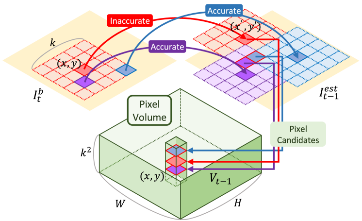
Figure 3. Pixel volume construction. A pixel $(x,y)$ in $I_{t}^{b}$ has $k^{2}$ matching candidates in $I_{t-1}^{est}$, where each pixel in the $k\times k$ window centered at $(x,y)$ gives one candidate. Pixel volume $V_{t-1}$ is a 3D volume containing the $k^{2}$ candidates for each pixel of $I_{t}^{b}$. For a pixel $(x,y)$, even when the matching candidate determined by BIMNet is inaccurate, the pixel pile of $V_{t-1}$ at $(x,y)$ may contain a correct match.

Previous video deblurring methods (Su et al., 2017; Kim et al., 2018) first align video frames by warping them before deblurring. However, during the warping process, structural artifacts may occur due to inaccurately estimated motion, which can eventually degrade the final deblurring results. To relieve this problem, Liao et al. (2015) proposed the draft-ensemble approach that computes multiple optical flow maps by using different regularization strengths so that correct motion for a local region can be estimated in some of the maps. However, this approach is computationally inefficient because it requires multiple optical flow estimation. To tackle the problem effectively and efficiently, we propose a novel pixel volume that does not require multiple optical flow estimation but can still provide multiple candidates for matching pixels between images.

For a pixel $(x,y)$ of $I_{t}^{b}$, we consider a spatial window of size $k\times k$ centered at $(x,y)$, where we fix $k=5$. For each pixel $(x+\Delta_{x},y+\Delta_{y})$ in the window, where $\Delta_{x},\Delta_{y}\in\{-\lfloor k/2\rfloor,...,\lfloor k/2\rfloor\}$, we have a matched pixel $(x^{\prime},y^{\prime})$ in $I_{t-1}^{est}$ determined by optical flow $W_{t-1}$. Then, its neighboring pixel $(x^{\prime}-\Delta_{x},y^{\prime}-\Delta_{y})$ in $I_{t-1}^{est}$ is a matching candidate for pixel $(x,y)$. Consequently, we have $k^{2}$ matching candidates in $I_{t-1}^{est}$ for $(x,y)$. We collect such matching candidates for all pixels in $I_{t}^{b}$ and stack them to obtain a pixel volume $V_{t-1}$ of size $W\times H\times k^{2}$, where $W$ and $H$ are the width and height of a video frame, respectively. The resulting pixel volume is in the form of a pile of $k^{2}$ images, where each image consists of pixels sampled from $I_{t-1}^{est}$, and the image for $(\Delta_{x},\Delta_{y})=(0,0)$ is the warping of $I_{t-1}^{est}$ by $W_{t-1}$. Fig. 3 illustrates the construction of a pixel volume.

The occurrence of multiple matching candidates in a pixel volume provide additional information that can reduce the deblurring artifacts caused by inaccurate motion estimation. Suppose that the pixel matching for $(x,y)$ determined by $W_{t-1}$ is incorrect due to small errors in motion estimation. Even in that case, if one of the $k^{2}$ neighbors of $(x,y)$ has a correct match, the pixel pile of $V_{t-1}$ at $(x,y)$ would contain a correct match for $(x,y)$. Moreover, a pixel volume provides an additional cue for motion compensation based on the majority. When the neighbors of a pixel have correct matches, the pixel volume can provide multiple duplicates of the correct match in the matching candidates for the pixel. Then, the majority cue can increase the reliability of motion compensation in deblurring the current frame $I_{t}^{b}$. In Sec. 4.4, we provide detailed statistics of candidate pixels in a pixel volume.

In short, our pixel volume approach leads to the performance improvement of video deblurring by utilizing the multiple candidates in a pixel volume in two aspects: 1) in most cases, the majority cue for the correct match would help as the statistics in Sec. 4.4 shows, and 2) in other cases, PVDNet would exploit multiple candidates to estimate the correct match referring to nearby pixels that have majority cues. This is a clear advantage over warping based alignment, because both majority cue and exploitation of multiple values cannot be provided by a single warped image that has only one candidate for each pixel.

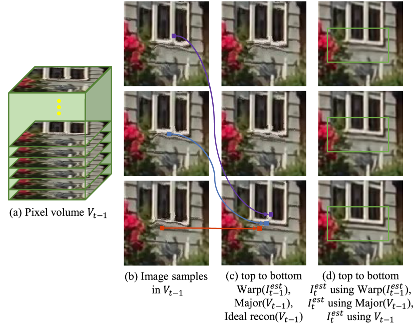
Figure 4. Robust deblurring with a pixel volume. Due to motion estimation errors, both naïve warping and majority-based warping of the deblurred previous frame $I_{t-1}^{est}$ contain artifacts ((c) top and middle). As a result, the variants of PVDNet using such warped frames produce deblurred results with remaining blur ((d) top and middle). In contrast, despite the motion estimation errors, our pixel volume contains enough information to reconstruct the ideal warping of $I_{t-1}^{est}$ ((c) bottom). Our PVDNet utilizes the information in the pixel volume to produce a high quality deblurred frame ((d) bottom).

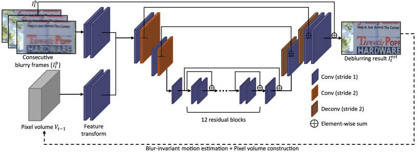
Figure 5. Architecture of PVDNet.

Fig. 4 compares motion compensation using warping and a pixel volume. The warped result of $I_{t-1}^{est}$ may contain deformation artifacts caused by motion estimation errors (Fig. 4c top). We also consider the majority-based warped result of $I_{t-1}^{est}$ (Fig. 4c middle). In majority-based warping, for each pixel, we choose the most frequent pixel value (the mode) among the $k^{2}$ candidates in a pixel volume. The majority-based warped frame contains similar artifacts to the simple warping result. In regions where the motion estimation results are inaccurate, the estimated flows are not consistent among neighboring pixels. Then, the most frequent values may not always be the best for motion compensation. As a result, the deblurring results obtained using such warped frames still contain a small amount of blur (Fig. 4d top and middle). In contrast, even in regions where motion estimation results are inaccurate, probably one or a few of the candidates in the pixel volume are correct. To demonstrate this phenomenon, we reconstructed an ideally warped image (Fig. 4c bottom) by choosing the most similar pixel to the ground truth sharp frame $I_{t}^{s}$ among the $k^{2}$ candidates for each pixel. The ideally warped image contains successfully reconstructed structures with less distortion, which shows the benefit of using a pixel volume. Consequently, the deblurring result obtained using the pixel volume (Fig. 4a) shows successfully restored sharp structures (Fig. 4d bottom). In Sec. B.4, we provide a quantitative analysis on the effect of a pixel volume.

Differences from relevant approaches

Our pixel volume construction scheme shares the same basis with the propagation step of the PatchMatch algorithm (Barnes et al., 2009): both methods exploit the spatial coherency of neighbor matches. However, our pixel volume scheme is distinct from PatchMatch in the following points. The PatchMatch propagation is designed to accelerate correspondence search, and therefore does not construct an explicit volume. Moreover, it is not straightforward to adopt PatchMatch to deep learning models. In contrast, our pixel volume scheme is specifically designed to improve the robustness of motion compensation and easily integrated into deep learning networks.

There have been other approaches relevant to our pixel volume scheme. Cho et al. (2012) also considered multiple candidates for video deblurring by using a window-based patch search. However, their method does not exploit the spatial coherency of neighbor matches, and is not designed for neural networks. Conventional stereo matching algorithms also construct a cost volume, but such cost volumes contain not pixel values but matching costs, and are therefore not directly applicable to video deblurring. Cost volumes do not exploit the spatial coherency of neighbor matches either.

3.3. Pixel volume based video deblurring network

PVDNet employs the U-Net (Ronneberger et al., 2015) architecture that has shown to be effective for deblurring (Nah et al., 2017; Su et al., 2017; Tao et al., 2018). We use symmetric skip-connections between the encoder and decoder to reconstruct a result image from encoded features while preserving image structures (Fig. 5). We add 12 residual blocks between the encoder and decoder to effectively refine blurry feature maps in low-resolution. We apply ReLU after all convolution and deconvolution layers except the layers that are connected by skip-connections; in these layers, the ReLU is applied after the summation of skip-connected features. We refer the readers to the appendix for a detailed architecture of PVDNet.

For early fusion of input images and a pixel volume, we add initial feature transform layers to the network. As aforementioned, our PVDNet takes four inputs (the previous, current, and next input frames, and pixel volume of the deblurred previous frame). Instead of directly concatenating the inputs, we transform and concatenate them using feature transform layers. We divide the inputs into two groups: the concatenated consecutive frames, and the pixel volume. We feed each group into the feature transform layers and fuse their features by concatenation. We use a grayscale pixel volume to reduce training and computational complexity. Our preliminary test shows that the model using a grayscale pixel volume has comparable performance to the model using a color pixel volume (Appendix B.2). The network has a long skip-connection from the input frame $I_{t}^{b}$ to the network output to make the network predict only residuals while preserving overall contents of the input frame.

To train PVDNet, we use mean absolute difference between deblurred frames and their corresponding ground truth sharp frames as the loss function. Although the network does not have any specific constraints or loss functions for temporal coherence, it generally produces temporally smooth results as our recurrent network utilizes the deblurred previous frame to process the current frame.

4. Experiments

4.1. Implementation and training details

To train both BIMNet and PVDNet, we used a dataset of synthetically blurred videos (Su et al., 2017), which was generated by capturing sharp videos at high frame rate, and averaging adjacent frames. The dataset consists of 71 pairs of a blurry video and its corresponding sharp video, which provide 6,708 pairs of 1280$\times$720 blurred and sharp frames in total. The videos in the dataset have blur caused by camera shake and object motion. We used 61 videos in the dataset as our training set, and 10 videos as our test set as Su et al. (2017) did. The training and test sets consist of 5,708 and 1,000 pairs of images, respectively.

Our training process consists of two steps. We first train BIMNet, and then PVDNet while fixing BIMNet. To train BIMNet, we fine-tuned LiteFlowNet (Hui et al., 2018) over the pre-trained weights provided by the authors. For fine-tuning, we randomly selected two consecutive frames from the training video set. We then randomly cropped the same areas of size $256\times 256$ from the selected frames, and fed them to the network. We used normalized pixel values from -1 to 1, and set the batch size to eight. We used Adam optimizer (Kingma and Ba, 2015) with $\beta_{1}=0.9$ and $\beta_{2}=0.999$. We initially set the learning rate to 0.0001, and decayed it with a decaying rate 0.1 for every 100,000 iterations. The network converged after $\sim$200,000 iterations. The training took about two days on a PC with an Nvidia GeForce TITAN-Xp (12GB).

To train PVDNet, we follow a conventional training strategy such as (Kim et al., 2017) to generate mini-batches for recurrent video processing. Specifically, we randomly sampled sequences of 13 consecutive frames from the training set. We sampled eight sequences, i.e., we used batch size of eight. Then, we randomly cropped the same areas of $256\times 256$ from the frames in each sequence. For each sequence, we iterate from the first to last cropped frame. For each iteration, we set the current cropped frame as the target blurry frame $I_{t}^{b}$ and compute the gradient using the result of the previous frame $I_{t-1}^{est}$ as well as the current target blurry frame and its neighboring blurry frames. Then, we update the network parameters by using backpropagation. The backpropagation is performed only for the current iteration, i.e., the gradient does not propagate to the network at the previous state through $I_{t-1}^{est}$. After iterating to the last frames, we repeat the process from the random sampling of video frame sequences. For the initial frame of each sequence, we set $I_{t-1}^{est}=I_{t}^{b}$ and $I_{t-1}^{b}=I_{t}^{b}$. We used Adam optimizer with $\beta_{1}=0.9$ and $\beta_{2}=0.999$ as was done for BIMNet. We trained PVDNet for 400,000 iterations with a learning rate of 0.0001. Then, we further trained the network for 200,000 iterations with the learning rate of 0.000025. The training of PVDNet took about four days on the aforementioned environment.

We do not train BIMNet and PVDNet jointly, because we use the explicit blur-invariant loss for motion estimation learning. BIMNet had been already trained with highly accurate supervision based on ground truth sharp images, so end-to-end training of BIMNet and PVDNet together did not improve the accuracy or quality of video deblurring. Similarly, Gast and Roth (2019) reported that fixed pre-trained optical flow models (Dosovitskiy et al., 2015; Sun et al., 2018) can be used to improve video deblurring accuracy quite well without sophisticated joint training. It is also known that end-to-end training schemes do not always improve the model performances in various image processing tasks, such as object detection  (Ren et al., 2015; He et al., 2017), image super-resolution (Ge et al., 2018), and image inpainting (Ren et al., 2019).

Table 1. Quantitative comparison between BIMNet and other optical flow estimation methods on blurry video frames. We computed average errors between $I_{t}^{s}$ and $Warp(I_{t-1}^{s},W^{bb})$ in PSNR and SSIM, where $W^{bb}$ is the optical flow estimated from $I_{t}^{b}$ to $I_{t-1}^{b}$.

Model	Entire test set		Sharpest 10%		Blurriest 10%
	PSNR (dB)	SSIM	PSNR (dB)	SSIM	PSNR (dB)	SSIM
TVL1 (Sánchez et al., 2013)	28.20	0.890	30.73	0.924	25.08	0.784
FlowNet2 (Ilg et al., 2017)	27.85	0.903	29.75	0.923	25.79	0.864
LiteFlowNet (Hui et al., 2018)	27.64	0.895	29.99	0.923	24.64	0.833
FlowNet2SS	28.21	0.909	30.57	0.925	25.06	0.811
LiteFlowNetSS	27.91	0.893	30.12	0.923	24.89	0.830
FlowNet2∗∗	27.89	0.868	30.20	0.922	24.14	0.761
LiteFlowNet∗∗	27.23	0.811	30.06	0.906	24.07	0.753
BIMNetFN2	28.79	0.907	30.61	0.926	26.64	0.873
BIMNetLFN	28.43	0.900	30.29	0.923	26.03	0.853

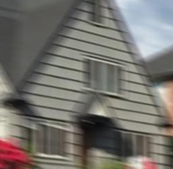
(a) $I_{t-1}^{b}$

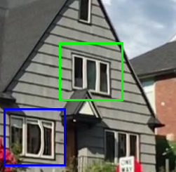
(b) FlowNet2

(c) FlowNet2_SS

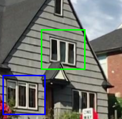
(d) BIMNet_FN2

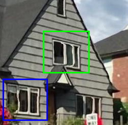
(e) TVL1

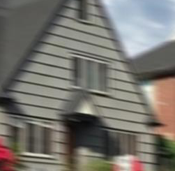
(f) $I_{t}^{b}$

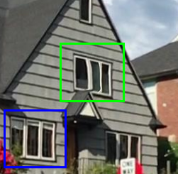
(g) LiteFlowNet

(h) LiteFlowNet_SS

(i) BIMNet_LFN

(j) GT

Figure 6. Qualitative comparison between BIMNet and other optical flow estimation methods. (a) and (f) are input blurry frames $I_{t-1}^{b}$ and $I_{t}^{b}$, respectively. From (b) to (i), we show the warped images $I_{t-1}^{{}^{\prime}s}=Warp(I_{t-1}^{s},W^{bb})$, where the optical flow maps $W^{bb}$ have been estimated from $I_{t-1}^{b}$ and $I_{t}^{b}$ by different methods.

4.2. Motion estimation performance

We first verify the effectiveness of our blur-invariant motion estimation learning by comparing our BIMNet with state-of-the-art optical flow estimation methods: TVL1 (Sánchez et al., 2013), FlowNet2 (Ilg et al., 2017), and LiteFlowNet (Hui et al., 2018). TVL1 is a traditional optimization-based approach. FlowNet2 improves FlowNet in terms of accuracy at the expense of an increased model size and slower computation. LiteFlowNet is a light-weight variant of FlowNet with a much reduced model size and faster computation. We considered two versions of BIMNet: BIMNet_FN2, which uses FlowNet2 network architecture; and BIMNet_LFN, which uses LiteFlowNet network architecture. BIMNet_LFN is the model adopted in our final framework. Our blur-invariant motion estimation learning uses blurry video frames and the blur-invariant loss in the training process. To verify the effect of each component, we consider four versions of FlowNet2 and LiteFlowNet: FlowNet2_SS, LiteFlowNet_SS, FlowNet2_∗∗, and LiteFlowNet_∗∗. FlowNet2_SS and LiteFlowNet_SS are fine-tuned versions of FlowNet2 and LiteFlowNet using sharp video frames in our training set, respectively. FlowNet2_∗∗ and LiteFlowNet_∗∗ are fine-tuned using all combinations of sharp and blurry video frames in our training set as done for BIMNet_FN2 and BIMNet_LFN. To fine-tune these variants, we did not use a blur-invariant loss in Eq. (1). Instead, we used the loss function defined as:

(2) $$L^{\alpha\beta}=MSE(Warp(I_{t-1}^{\alpha},W^{\alpha\beta}),I_{t}^{\beta}),$$

which is blur-variant, where $\alpha,\beta\in\{s,b\}$.

To measure the performance of each method, we measured the warping accuracy of motion estimation results. Specifically, we first estimated the optical flow from $I_{t}^{b}$ to $I_{t-1}^{b}$. We then obtained $I_{t}^{{}^{\prime}s}$ by warping $I_{t-1}^{s}$ with the computed optical flow, and measured the difference between the warping result $I_{t}^{{}^{\prime}s}$ and its ground truth sharp frame $I_{t}^{s}$, in terms of peak signal-to-noise ratio (PSNR) and structural similarity index (SSIM) (Wang et al., 2004). Following Su et al. (2017), to handle the ambiguity in the pixel location caused by blur, we measure PSNRs and SSIMs using an approach (Köhler et al., 2012) that first aligns two images using global translation. To analyze the performance of different methods on blurry videos more clearly, we also measured the performance on the sharpest 10% and the blurriest 10% video frames in each video in the test set. To choose the sharpest and blurriest 10% frames, we measured the blurriness of all test frames as PSNRs between blurry frames and their corresponding sharp ground truth frames. We assume that a test frame with a low PSNR is likely to have large blur, because blur is the primary factor of structural differences from its ground truth.

Table 1 shows a summary of the quantitative comparison using our test set. For the entire test set, BIMNet_FN2 and BIMNet_LFN achieve the best and second-best PSNR and comparable SSIM. The result shows that BIMNet_FN2 significantly outperforms the other methods on the severely blurred frames by a large margin, while it performs comparably on the relatively sharp frames. BIMNet_LFN was slightly inferior to BIMNet_FN2, but still outperforms all the other methods. Moreover, BIMNet_LFN has only 5.4M parameters, whereas BIMNet_FN2 has 150M parameters. Thus, we adopt BIMNet_LFN for our framework.

To identify the source of the improvement of BIMNet, we compared FlowNet2, FlowNet2_SS, FlowNet2_∗∗, and BIMNet_FN2. Compared to FlowNet2, FlowNet2_SS shows improvement for relatively sharp frames, but yields inferior results for blurry frames as a result of overfitting to sharp video frames. FlowNet2_∗∗ performs worse than FlowNet2_SS for both sharp and blurry frames; this result shows that simply including blurry frames in training does not improve the accuracy of optical flow estimation on blurry frames. Compared to these, BIMNet_FN2 that is trained using our blur-invariant loss shows improvements in all cases. A similar trend can also be found from LiteFlowNet_SS, LiteFlowNet_∗∗, and BIMNet_LFN. This result verifies that our blur-invariant loss is the source of the improvement in motion estimation accuracy in the presence of blur.

Fig. 6 shows a qualitative comparison of different optical flow methods. To visually compare the quality of different optical flow methods, we estimated optical flow maps between two consecutive blurred video frames, $I_{t-1}^{b}$ and $I_{t}^{b}$, using different optical flow methods, and warped the sharp video frame $I_{t-1}^{s}$ corresponding to $I_{t-1}^{b}$ using the estimated optical flow maps. As the figure shows, the results of the other methods contain severely distorted structures due to errors in their optical flow maps. In contrast, the results of BIMNet_FN2 and BIMNet_LFN show much less distortions.

4.3. Ablation study

To show the effectiveness of the BIMNet and pixel volume in our video deblurring framework, we performed an ablation study. We tested five models in this study. The baseline is PVDNet that receives consecutive blurry frames as well as a deblurred previous frame without any motion compensation. Then, one by one, we add motion compensation (MC) using LiteFlowNet_SS, blur-invariant motion compensation (BIMC) using BIMNet_LFN, and pixel volume (PV) into the baseline model. Another straightforward idea to increase the performance is to jointly train motion estimation and deblurring. To verify the effectiveness of our BIMC against such a joint approach, we also include a jointly trained model (MC_e2e + PV) in which the motion estimation module is first initialized by LiteFlowNet_SS and then jointly trained with PVDNet by using the deblurring loss in an end-to-end manner.

Our model that uses BIMC and PV shows the best PSNR and SSIM (Table 2). For the sharpest 10% of the frames of each video in the test set, all the models, even the baseline model without motion compensation, show high performances. In contrast, for the blurriest 10% of the frames, each of BIMC and PV achieves drastic improvement over the models with and without MC; these results indicate that BIMC and PV are effective for handling large blur. The table also shows that joint training of motion estimation and PVDNet (MC_e2e + PV) does not increase but decreases the deblurring performance compared to MC + PV. This result occurs because the deblurring loss does not provide good guidance for accurate motion estimation, and the loss adversarially affects its training.

Fig. 7 shows a qualitative comparison. The models without BIMC cannot compensate for large motions, and therefore did not well restore the big red characters in the blue box. The models without PV cannot compensate for small distortions caused by motion estimation errors, and did not properly recover the small black characters in the green box. Our full model with BIMC and PV could deblur successfully in both cases, and produced the best results.

Table 2. Ablation study for video deblurring performance. PSNR are in dB.

Model	Entire test set		Sharpest 10%		Blurriest 10%
	PSNR	SSIM	PSNR	SSIM	PSNR	SSIM
input	27.40	0.819	33.02	0.936	22.77	0.665
baseline	30.66	0.891	34.76	0.954	26.15	0.780
MC	31.23	0.901	35.10	0.957	26.69	0.798
BIMC	31.46	0.912	35.15	0.958	27.28	0.820
MC + PV	31.40	0.910	35.13	0.958	27.19	0.817
MCe2e + PV	31.32	0.909	34.95	0.956	27.21	0.818
BIMC + PV	31.63	0.915	35.18	0.958	27.46	0.828

Input
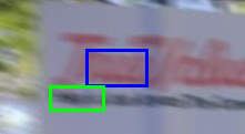
Baseline
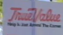
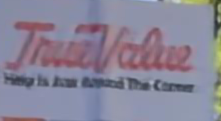
MC
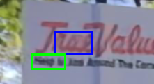
BIMC
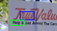
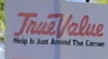
MC+PV
BIMC+PV

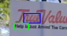
Figure 7. Qualitative comparison of the models in Table 2 for three consecutive video frames.

4.4. Statistics of candidate pixels in pixel volume

From each video in the test set of (Su et al., 2017), we sampled ten frames, and gathered 100 frames. We then constructed PVs for those frames, and investigated the distribution of pixel values in the volumes. In the PVs, 95.1% of the pixels had majority values in the candidates, where a majority value means more than a half of the $k^{2}$ candidates for a pixel have the same value. We then investigated the accuracy of those majority values. As our PVs are constructed from deblurred previous frames, they may not have perfect matches with ground truth pixel values. Thus, to measure the accuracy, we counted the number of majority values that are close enough to the ground truth pixel values, i.e., the pixel value differences are within $\pm c$ in 0-255 scale. The accuracy of those majority values was 89.5% when $c$ = 0 (perfect match) and increased to 92% for $c$ = 2.

While most of the pixels in the pixel volume have correct majority values, the pixel volume is still helpful even for deblurring regions that have no majority values or wrong ones. To validate it, we measured the accuracy of deblurring results on those regions using two models: one that uses PV, and the other that uses naïve warping. The accuracy was measured in the same way as above with $c$ = 2. In regions where the majority values are correct, the model that uses PV achieved accuracy of 97.42%, and the model that uses naïve warping achieved 96.91%. For regions in which majority values are wrong, the model that uses PV (57.35%) shows a significantly higher accuracy than the model that uses naïve warping (50.49%). Likewise, for the region that has no majority values, the model that uses PV (89.97%) also shows higher accuracy than the model that uses naïve warping (87.77%). This result confirms that our PV helps our deblurring network obtain the correct values even when the majority pixels in the PV are wrong.

4.5. Motion compensation vs. larger model

Our method adopts an additional motion estimation network, BIMNet, so the accuracy gain could be simply a result of increasing the total model size. To investigate on this possibility, we prepared variants of our deblurring framework with different model sizes either with or without motion compensation. Specifically, we prepared small, medium, and large versions of PVDNet. The medium model is the model described in Sec. 3.3. The small model has half the number of filters in every convolution layer, and half the number of residual blocks of the medium model. The large model has twice the number of filters in every convolution layer. Then, we prepared six variants of our framework either with or without our motion compensation scheme that combines BIMNet and PV, and measured the models’ deblurring accuracies.

Table 3 shows that the small and medium models with our motion compensation scheme outperformed the large model without motion compensation despite their significantly smaller model sizes. Fig. 8 also shows that the small and medium models with motion compensation could recover small-scale structures and textures better than the large model without motion compensation. Both quantitative and qualitative comparisons clearly show the superiority of our motion compensation scheme over simply increasing the size of the model.

Table 3. Performance comparison of PVDNets with different model sizes either with or without MC. The unit of the number of parameters is million (M). Values in the parentheses are the numbers of parameters of PVDNet and BIMNet.

Model	PSNR (dB)	SSIM	Parameters (M)
Small	30.03	0.880	0.7
Medium	30.66	0.891	5.1
Large	30.85	0.898	19.6
Small + MC	30.95	0.904	6.1 (0.7 + 5.4)
Medium + MC	31.63	0.915	10.5 (5.1 + 5.4)
Large + MC	31.75	0.918	25.0 (19.6 + 5.4)

Table 4. Quantitative comparison of our video deblurring framework with recent state-of-the-art methods on the dataset of (Su et al., 2017). Values in the parentheses are the numbers of parameters or computations of PVDNet and BIMNet. For DVD-MC, the numbers of parameters and computations for motion estimation are not included, as DVD-MC does not use a deep learning-based model for motion estimation. CA denotes the cosine annealing scheduling method for learning rate (Loshchilov and Hutter, 2017), which EDVR adopts for its training.

	PSNR (dB)	SSIM	Parameters (M)	Computations (BMACs)
(Nah et al., 2017)	29.85	0.880	75.7	2364
(Tao et al., 2018)	30.53	0.894	3.8	1175
DVD-noMC (Su et al., 2017)	30.29	0.888	15.3	557
DVD-MC (Su et al., 2017)	30.47	0.898	15.3	557
OVD (Kim et al., 2017)	30.08	0.873	0.9	206
IFI-RNN (Nah et al., 2019)	31.04	0.903	1.6	200
IFI-RNN-L (Nah et al., 2019)	31.67	0.916	12.2	1,425
EDVR (Wang et al., 2019)	31.82	0.916	23.6	2,739
Ours-small	31.25	0.908	6.1 (0.7 + 5.4)	424 (105 + 319 )
Ours	31.95	0.920	10.5 (5.1 + 5.4)	936 (617 + 319)
Ours w/ CA	32.31	0.926	10.5 (5.1 + 5.4)	936 (617 + 319)

4.6. Comparison with other deblurring methods

We compared our method with six recent state-of-the-art deep learning based deblurring methods, including two single image-based methods (Nah et al., 2017; Tao et al., 2018), and four video deblurring methods (Su et al., 2017; Kim et al., 2017; Nah et al., 2019; Wang et al., 2019). For the single image deblurring methods of Nah et al. (2017) and Tao et al. (2018), we applied them to each input frame independently. The method of Su et al. (2017) takes consecutive blurry video frames as input, which can be either motion compensated using optical flow or not. In our comparison, we included both versions with and without motion compensation, which are denoted by DVD-MC and DVD-noMC, respectively. For motion compensation for DVD-MC, we used the method of Sánchez et al. (2013) as done in (Su et al., 2017). The method of Wang et al. (2019), which we refer to as EDVR, also takes consecutive blurry video frames as input. The methods of Kim et al. (2017) and Nah et al. (2019), which we refer to as OVD and IFI-RNN, respectively, adopt recurrent network structures that take an intermediate feature map of the previous frame without motion compensation.

For fair comparison in terms of model size, we also included a variant of IFI-RNN with an increased model size, which we refer to as IFI-RNN-L, and a smaller version of our framework (the small PVDNet in Sec. 4.5), which we refer to as Ours-small. IFI-RNN-L has twice the number of residual blocks and also twice the number of channels in every convolution layer. Finally, for fair comparison with EDVR, we also include another variant of our framework (Ours w/ CA), which is trained using cosine annealing (CA) (Loshchilov and Hutter, 2017), a sophisticated learning rate scheduling strategy adopted to EDVR.

For evaluation, we used three test sets in the comparison. Specifically, in addition to Su et al. (2017)’s dataset, we used another popular video deblurring dataset (Nah et al., 2017), synthetically generated in a similar way to Su et al. (2017)’s dataset. We also used real-world videos (Su et al., 2017) to check the generalization ability of our model.

(a) Input	(b) Large	(c) Small + MC	(d) Medium + MC

Figure 8. Qualitative comparison of PVDNets with different model sizes either with or without MC. The small and medium PVDNets with MC restore image details better than the large PVDNet, showing that MC is more effective than simply increasing the model size.

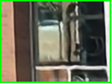
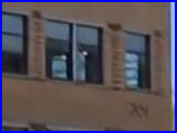
(a) Input		(b) (Tao et al., 2018)		(c) DVD-MC (Su et al., 2017)		(d) EDVR (Wang et al., 2019)
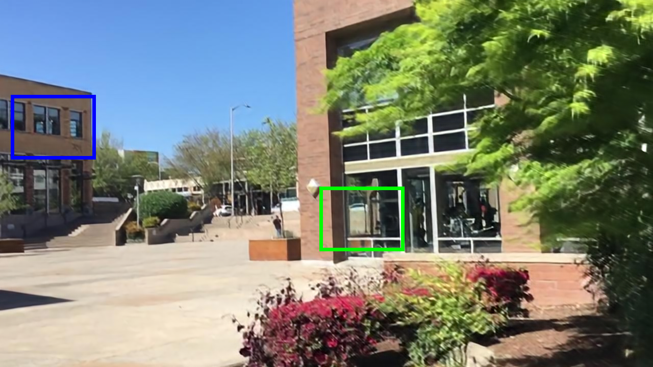
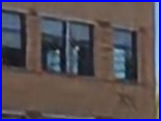
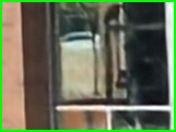
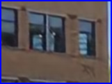
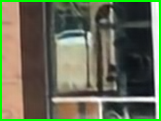
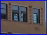
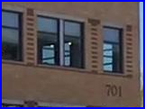
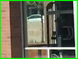
(e) IFI-RNN (Nah et al., 2019)		(f) IFI-RNN-L (Nah et al., 2019)		(g) Ours		(h) GT

Figure 9. Qualitative comparison on synthetically blurred video frames of Su et al. (2017)’s dataset.

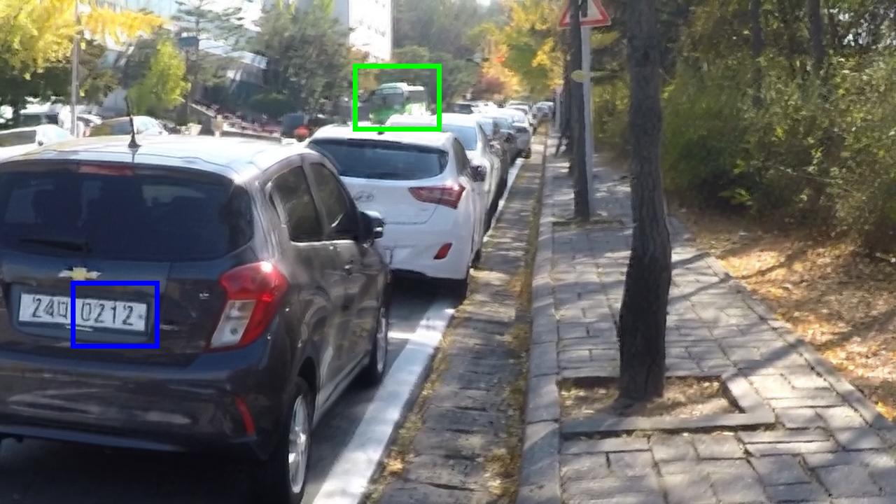
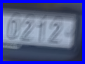
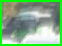
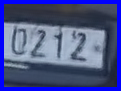
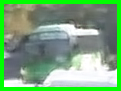
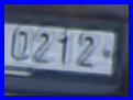
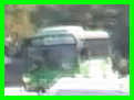
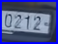
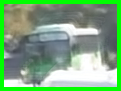
(a) Input		(b) (Nah et al., 2017)		(c) (Tao et al., 2018)		(d) EDVR (Wang et al., 2019)
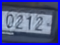
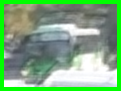
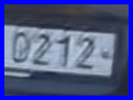
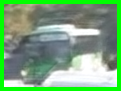
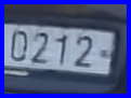
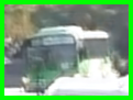
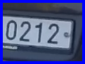
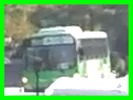
(e) IFI-RNN (Nah et al., 2019)		(f) IFI-RNN-L (Nah et al., 2019)		(g) Ours		(h) GT

Figure 10. Qualitative comparison on synthetically blurred video frames of Nah et al. (2017)’s dataset.

Comparison using Su et al. (2017)’s dataset

For fair comparison, we trained all the models except for OVD (Kim et al., 2017) and DVD (Su et al., 2017) using the dataset of Su et al. (2017). For this training, we used the source code provided by the authors and their own training strategies. The training code of OVD is not available, so we used its pre-trained model provided by the authors. We also used the model of DVD provided by the authors; it had already been trained with Su et al.’s dataset. For quantitative evaluation, we excluded the first frames of test videos, because most video deblurring methods cannot successfully handle them.

In the quantitative comparison (Table 4), our model achieved higher PSNR and SSIM than all the other methods, including single image and video deblurring methods. Compared to both DVD-noMC and DVD-MC, even Ours-small performed much better despite its significantly smaller size, because DVD cannot utilize previous deblurred frames due to the lack of a recurrent structure. Compared to OVD, Ours-small achieved PSNRs more than 1 dB higher. Ours-small has more parameters than OVD, but most are used for motion estimation; the deblurring network, PVDNet, has fewer parameters than OVD. This comparison clearly shows the benefit of our motion compensation scheme. Similarly, compared to IFI-RNN, Ours-small as well as Ours outperformed it both in PSNR and SSIM, in spite of the smaller deblurring network. Compared to IFI-RNN-L and EDVR, which have larger numbers of parameters, Ours achieved higher PSNR and SSIM even though the total number of parameters is smaller. Finally, Ours trained with CA outperformed EDVR by a margin of 0.49 dB, proving the effectiveness of our framework.

The advantage of our approach is emphasized in the qualitative comparison (Fig. 9). As the input video frame (Fig. 9a) is severely blurred, the single image deblurring method of Tao et al. (2018) fails to recover fine-scale structures and produces blurry results. DVD-MC recovers fine-scale structures better, but produces distorted structures due to motion compensation errors. IFI-RNN, IFI-RNN-L, and EDVR also fail to restore fine-scale structures due to large motions in the input frames. In contrast, thanks to our motion compensation scheme, our method effectively restores fine details without distortions even in the presence of large inter-frame motion and blur.

Comparison using Nah et al. (2017)’s dataset

For fair comparison, all the methods except for OVD (Kim et al., 2017) were trained from scratch with the training set of Nah et al. (2017). In the quantitative comparison (Table 5), our method using cosine annealing (Ours w/ CA) achieved better or comparable performance to the other state-of-the-art methods including IFI-RNN-L (Nah et al., 2019) and EDVR (Wang et al., 2019) despite its smaller model size. In this comparison, we also included our method with a similar model size to that of EDVR, to show the effectiveness of our explicit motion compensation approach. Specifically, to increase the model size to match that of EDVR, we used a larger PVDNet that has 24 residual blocks with 192 channels. Our larger model (Ours-large w/ CA) clearly outperforms EDVR both in PSNR and SSIM.

In a qualitative comparison, the input blurred frame (Fig. 10a) has severe blur caused by large camera motion. Consequently, the results of all the other methods have remaining blur. On the other hand, our result (Fig. 10g) shows clearly restored details with no remaining blur.

Table 5. Quantitative comparison of our video deblurring framework with recent state-of-the-art methods on the dataset of (Nah et al., 2017).

	PSNR (dB)	SSIM	Parameters (M)
(Nah et al., 2017)	29.47	0.876	75.7
(Tao et al., 2018)	30.61	0.908	3.8
OVD (Kim et al., 2017)	26.57	0.820	0.9
IFI-RNN (Nah et al., 2019)	30.15	0.895	1.6
IFI-RNN-L (Nah et al., 2019)	31.05	0.911	12.2
EDVR (Wang et al., 2019)	31.54	0.926	23.6
Ours	31.30	0.917	10.5 (5.1 + 5.4)
Ours w/ CA	31.52	0.921	10.5 (5.1 + 5.4)
Ours-large w/ CA	31.98	0.928	23.4 (18.0 + 5.4)

Comparison using real-world videos

Finally, we qualitatively compare the performance of our approach to those of the state-of-the-art methods on real-world data (Fig. 11). The datasets (Su et al., 2017; Nah et al., 2017) that were used for training and evaluation are synthetically generated using high-speed cameras, so it may not fully represent the characteristics of real blurry videos. Thus, evaluation using real-world data is essential for predicting the generalization ability of a method. For evaluation, we used the real blurry video test set in Su et al. (2017).

In this comparison, the input video frame (Fig. 11a) is severely blurred by camera motions, so the characters in the frame are illegible. The single image deblurring method of Tao et al. (2018) (Fig. 11b) failed to restore the characters properly and introduced noisy artifacts. The results of the video deblurring methods, DVD-MC (Fig. 11c) and IFI-RNN (Fig. 11e) have remaining blurs. Compared to the results of the other methods, the results of EDVR (Fig. 11d) and IFI-RNN-L (Fig. 11f) show relatively better restored details because of their large model sizes, but small characters remain illegible either. In contrast, both Ours-small (Fig. 11g) and Ours (Fig. 11h) more clearly restore characters with less artifacts despite their smaller models than EDVR and IFI-RNN-L.

In another qualitative comparison (Fig. 12), the input video frames suffer from large blur. DVD-MC restored small-scale structures relatively well, but its results still have remaining blur and noisy artifacts. IFI-RNN-L completely failed to restore sharp frames, possibly due to large motions between input frames that are difficult to handle without explicit motion compensation. On the contrary, our results clearly restored sharp details. Additional examples can be found in the supplementary material.

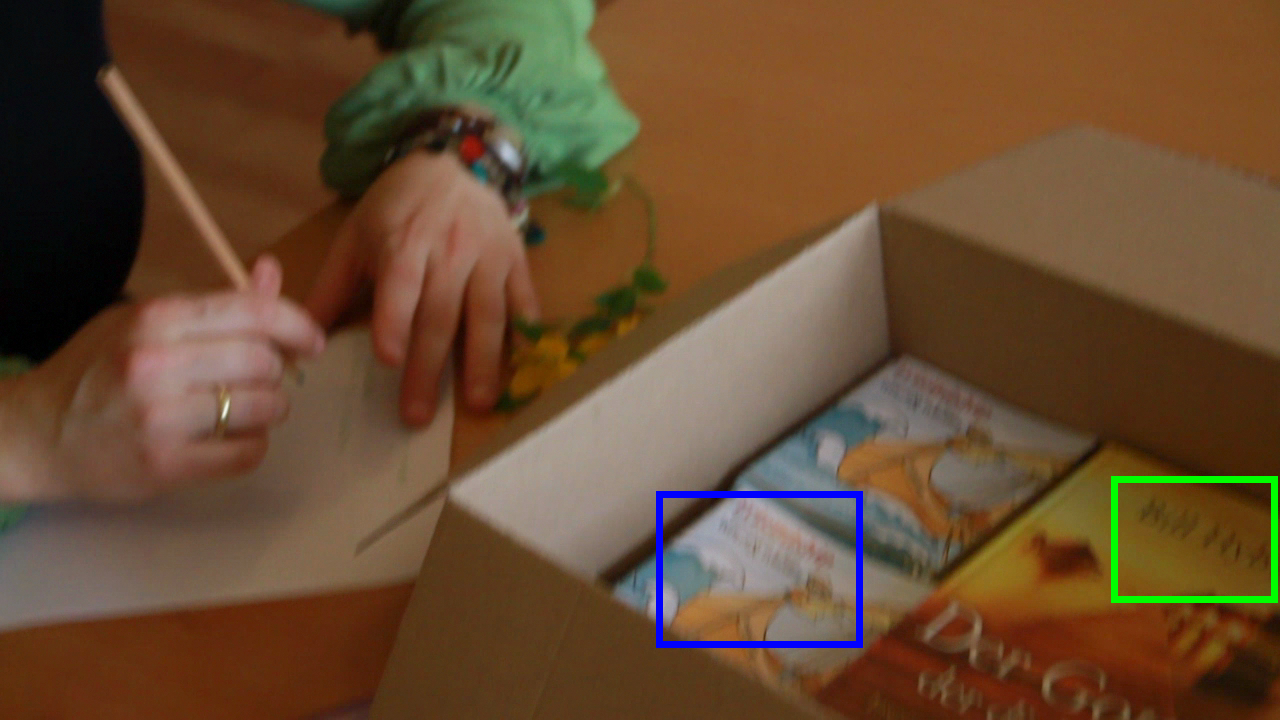
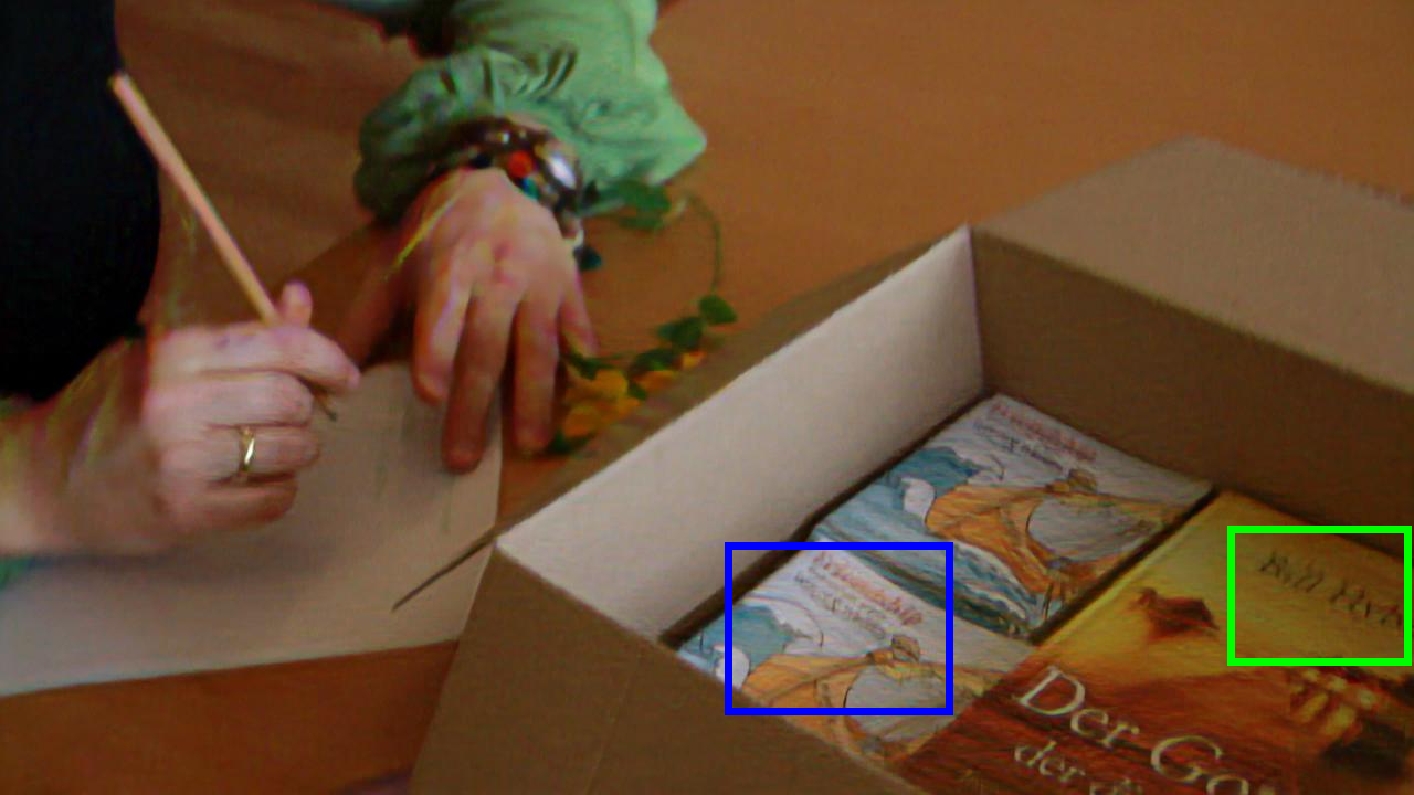
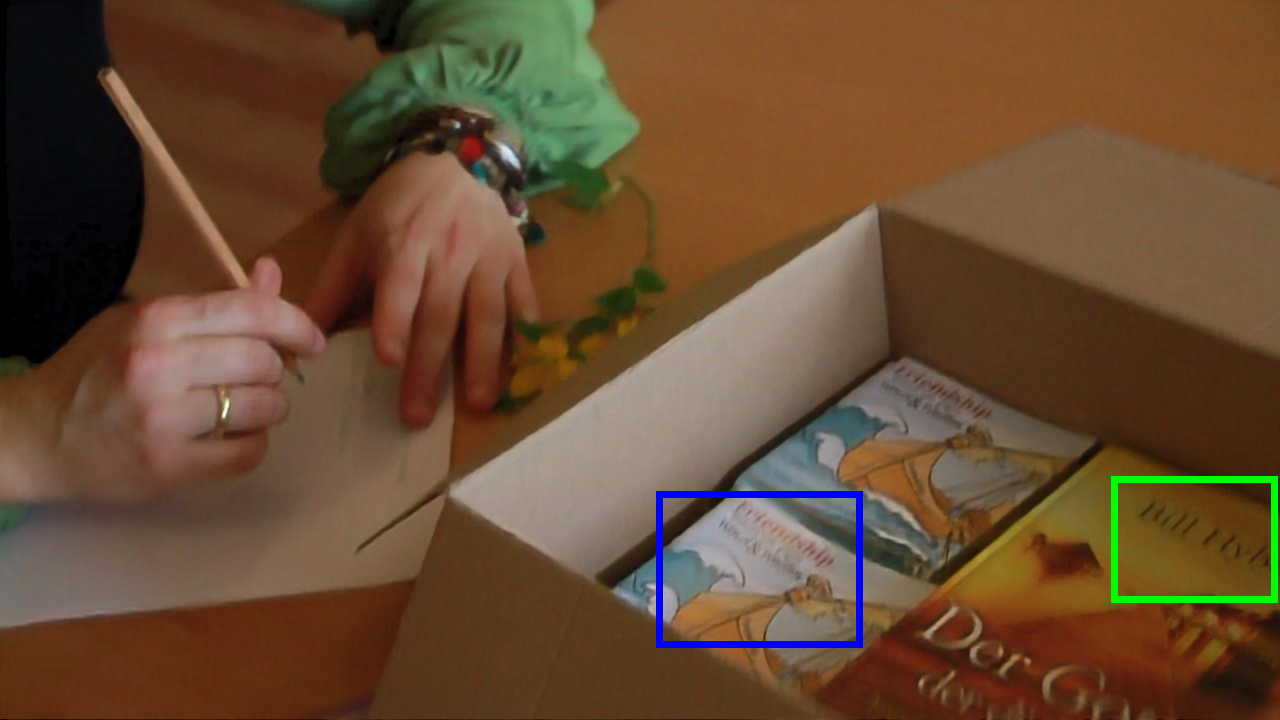
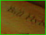
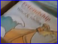
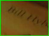
(a) Input		(b) (Tao et al., 2018)		(c) DVD-MC (Su et al., 2017)		(d) EDVR (Wang et al., 2019)
		3.8M params		15.3M params		23.6M params
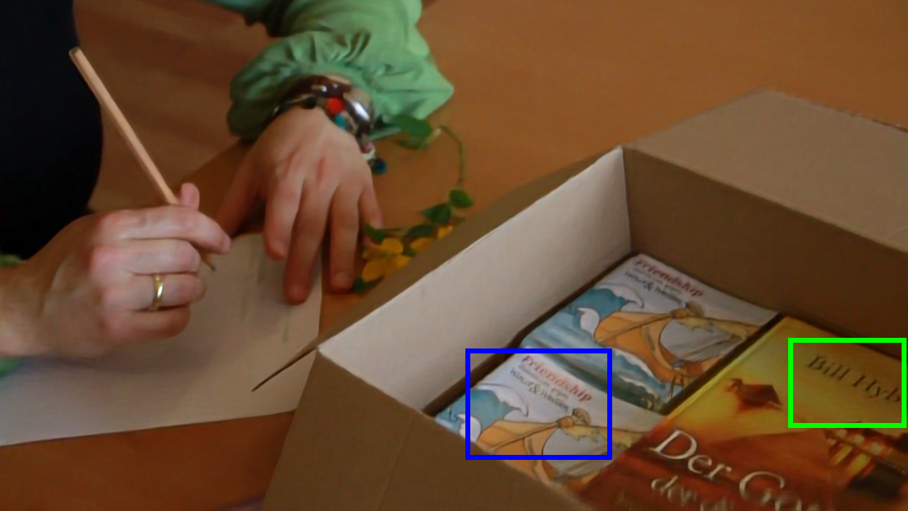
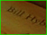
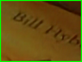
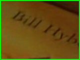
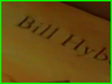
(e) IFI-RNN (Nah et al., 2019)		(f) IFI-RNN-L (Nah et al., 2019)		(g) Ours-small		(h) Ours
1.6M params		12.2M params		6.1M (0.7M + 5.4M) params		10.5M (5.1M + 5.4M) params

Figure 11. Qualitative comparison on real-world video frames of Su et al. (2017)’s test set.

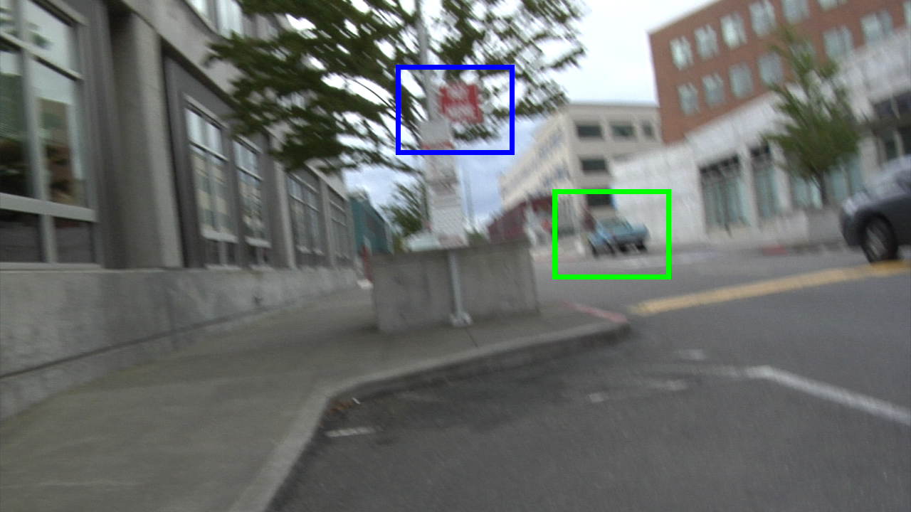
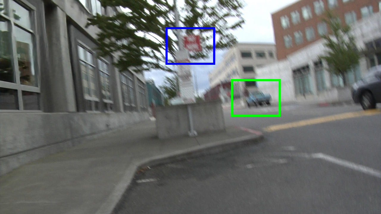
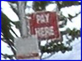
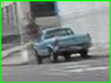
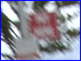
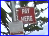
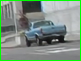
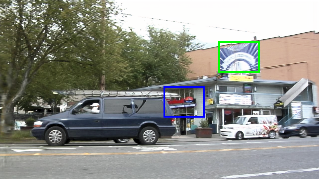
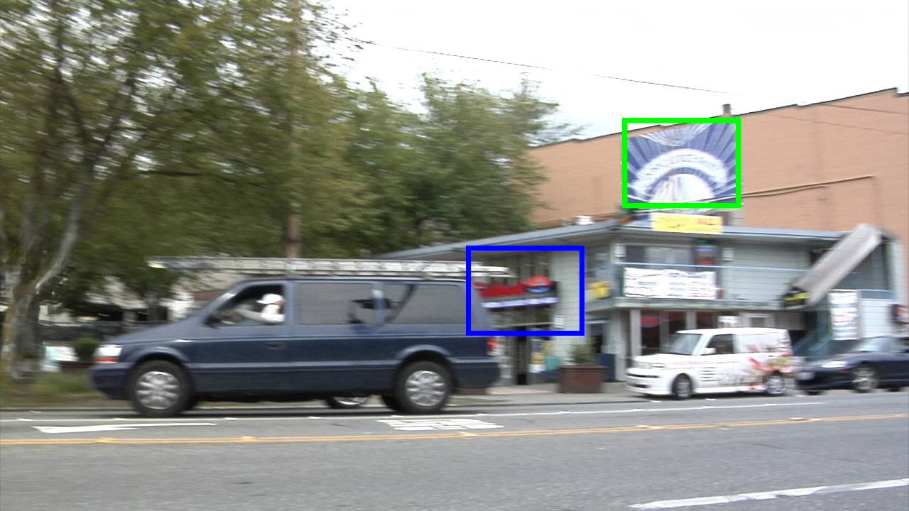
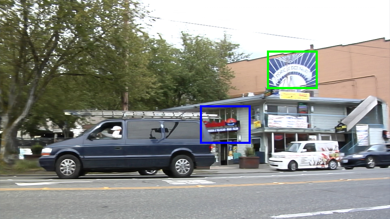
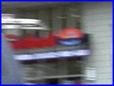
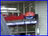
(a) input		(b) DVD-MC (Su et al., 2017)		(c) IFI-RNN-L (Nah et al., 2019)		(d) Ours

Figure 12. Additional examples on real-world video frames of Su et al. (2017)’s test set.

4.7. Computational cost analysis

To process a single 1280$\times$720 video frame, our framework takes about 0.11s with an NVIDIA Titan Xp GPU, and our framework can process images of arbitrary size, because both BIMNet and PVDNet consist of convolutional layers. Specifically, BIMNet, PVDNet, and pixel volume construction take 0.04s, 0.04s, and 0.03s per frame, respectively. The pixel volume construction step takes relatively long computation time. However, its code is un-optimized PyTorch code that uses for-loops, which are known to be slow in PyTorch. We believe that the code can be further optimized using CUDA programming. The computational overhead caused by a pixel volume in PVDNet is smaller than that of a single convolution layer in our framework. In the aspect of memory usage, the size of a pixel volume is $W\times H\times k^{2}$, and $k$ is set to 5 in our experiments. In contrast, the first convolution layer of PVDNet uses 64 channels so its size is $W\times H\times 64$. Thus, a PV requires only $\sim$39% memory usage of the first convolution layer. In the aspect of computation time, once a pixel volume is constructed, it is processed by convolution operations like other layers. Thus, the overhead computation time caused by a pixel volume is also smaller than that of a single convolution layer in our framework.

We compared the computational costs of our method and others. We used the number of Multiply-accumulate (MAC) operations required to process a single 1280$\times$720 video frame as the measurement. Our method (936 BMACs) has a much smaller computational cost than IFI-RNN-L (1425 BMACs) and EDVR (2739 BMACs) despite achieving higher deblurring accuracy (Table 4).

5. Conclusion

In this paper, we presented two novel approaches for motion compensation to effectively deliver previously deblurred information. We proposed simple but effective blur-invariant learning for accurate estimation of optical flow between blurred video frames. In addition, we constructed a pixel volume that contains matching candidates for robustly handling motion estimation errors, and fed it to our deblurring network instead of directly feeding a motion compensated warped frame. Finally, we proposed an effective video deblurring framework based on the proposed motion compensation approaches.

Our framework achieved the state-of-the-art deblurring performance, as demonstrated by extensive experiments on various challenging videos with large blur. Combination of blur-invariant motion estimation learning and a pixel volume can improve motion compensation without significant computational overhead or changes in network design. We expect that these two modules would be applicable to other video processing tasks, such as video super-resolution that requires sub-pixel-level motion compensation.

Similarly to previous deblurring methods (Nah et al., 2017; Tao et al., 2018; Su et al., 2017; Kim et al., 2017, 2018; Wang et al., 2019), in the synthetic datasets (Su et al., 2017; Nah et al., 2017), we use temporal center frames as ground truth sharp frames for training both BIMNet and PVDNet. However, complex blur such as circular blur may introduce ambiguity, because more than one camera motions with different temporal centers can produce the same shape of blur; this ambiguity may confuse the networks and degrade their performances. This problem would not be severe in practice given the success of recent deblurring methods that use temporal center frames for ground truths, but analyzing its effect and resolving it can be a good future direction.

Appendix

Appendix A BIMNet

A.1. Effect of Siamese structure on blur-invariant feature learning

As described in Sec. 3.1, we adopt LiteFlowNet (Hui et al., 2018) for our BIMNet as LiteFlowNet has a Siamese network architecture that is effective to learn blur-invariant features. In this section, we conduct an experiment to verify the effectiveness of the Siamese architecture on blur-invariant feature learning.

To this end, we compare two different networks for optical flow estimation: FlowNetS and FlowNetC (Dosovitskiy et al., 2015). FlowNetS and FlowNetC share almost the same network architecture except that FlowNetC has a Siamese network at the beginning of the network, while FlowNetS has a plain CNN architecture. Using the Siamese network architecture, FlowNetC first extracts a feature for each pixel and then match the extracted features to estimate optical flow. While both FlowNetS and FlowNetC can run as stand-alone networks for optical flow estimation, LiteFlowNet combines them together for obtaining high-quality optical flow.

To investigate the effect of the Siamese network architecture, we evaluated the performance of FlowNetS and FlowNetC on blur-invariant feature learning. Specifically, we fine-tuned both pretrained networks with our blur-invariant loss $L_{BIM}^{\alpha\beta}$. The networks were originally pre-trained with datasets of (Geiger et al., 2012; Scharstein et al., 2014; Butler et al., 2012) and we used the dataset of Su et al. (2017) for fine-tuning them. Table 6 compares FlowNetS and FlowNetC with their fine-tuned versions. While $L_{BIM}^{\alpha\beta}$ improves the accuracy of both networks for blurry videos, the improvement of FlowNetC is much larger than that of FlowNetS, showing that the Siamese network architecture of FlowNetC learns to extract blur-invariant features more effectively than a plain CNN architecture.

Table 6. Accuracy gain of a Siamese structure in blur-invariant feature learning. The networks with subscript $L_{BIM}^{\alpha\beta}$ are fine-tuned ones with blur-invariant loss $L_{BIM}^{\alpha\beta}$ on the training set of Su et al. (2017). We computed the errors between $I_{t}^{s}$ and $Warp(I_{t-1}^{s},W^{bb})$ using PSNR and SSIM for each network, where $W^{bb}$ is the optical flow estimated from $I_{t}^{b}$ to $I_{t-1}^{b}$. Errors were measured on the test set of Su et al. (2017). Accuracy gain is higher for FlowNetC${}_{L_{BIM}^{\alpha\beta}}$ than FlowNetS${}_{L_{BIM}^{\alpha\beta}}$.

Model	PSNR (dB)	SSIM
FlowNetS	25.8619	0.8653
FlowNetS${}_{L_{BIM}^{\alpha\beta}}$	26.7387	0.8792
accuracy gain	3%	1%
FlowNetC	26.0403	0.8659
FlowNetC${}_{L_{BIM}^{\alpha\beta}}$	27.7182	0.9179
accuracy gain	6%	6%

Table 7. Quantitative comparison between BIMNet and other optical flow estimation methods on different types of image pairs $(I_{t-1}^{\alpha},I_{t}^{\beta})$. We computed average errors between $I_{t}^{s}$ and $Warp(I_{t-1}^{s},W^{\alpha\beta})$ in PSNR and SSIM, where $W^{\alpha\beta}$ is the optical flow estimated from $I_{t}^{\alpha}$ to $I_{t-1}^{\beta}$. BS, SB, and SS denote $(\alpha,\beta)$: $(b,s)$, $(s,b)$, and $(s,s)$, respectively.

Model	BS		SB		SS
	PSNR (dB)	SSIM	PSNR (dB)	SSIM	PSNR (dB)	SSIM
TVL1 (Sánchez et al., 2013)	27.34	0.869	28.08	0.875	30.78	0.904
FlowNet2 (Ilg et al., 2017)	28.22	0.903	28.04	0.898	30.03	0.928
LiteFlowNet (Hui et al., 2018)	27.47	0.882	26.51	0.858	29.49	0.923
FlowNet2SS	27.41	0.869	27.76	0.864	30.95	0.910
LiteFlowNetSS	27.90	0.885	27.57	0.874	30.64	0.927
FlowNet2∗∗	27.86	0.824	27.33	0.837	30.64	0.868
LiteFlowNet∗∗	27.02	0.811	26.83	0.789	29.76	0.887
BIMNetFN2	28.98	0.909	29.29	0.910	30.68	0.928
BIMNetLFN	28.85	0.901	28.86	0.901	30.64	0.928

A.2. Performance of BIMNet on different types of image pairs $(I_{t-1}^{\alpha},I_{t}^{\beta})$

Sec. 4.2 verified the effectiveness of our blur-invariant motion estimation learning by comparing BIMNet with state-of-the-art optical flow estimation methods, by measuring PSNR and SSIM between $Warp(I_{t-1}^{s},W^{bb})$ and $I_{t}^{s}$. In this section, we provide an additional evaluation of the performance of BIMNet on images with different types of blur. Specifically, we evaluated the performance of BIMNet for the other three cases: BS $(Warp(I_{t-1}^{s},W^{bs}),I_{t}^{s})$, SB $(Warp(I_{t-1}^{s},W^{sb}),I_{t}^{s})$, and SS $(Warp(I_{t-1}^{s},W^{ss}),I_{t}^{s})$.

Table 7 shows the evaluation results of BS, SB, and SS. In the cases of BS and SB, BIMNet_FN2 and BIMNet_LFN achieved the best and second-best performances, respectively, in both PSNR and SSIM, clearly outperforming all the other methods. In the case of SS, while FlowNet2_SS, which is trained for sharp images, performs the best in PSNR, BIMNet_FN2 and BIMNet_LFN perform comparably in PSNR and better than the other methods in SSIM, showing that both of them perform reasonably well even for sharp images.

Appendix B PVDNet

B.1. Network architecture

A detailed architecture of PVDNet is given in Table 8.

B.2. Preliminary tests for PVDNet

As described in Sec. 3, our framework takes neighboring frames $I_{t-1}^{b}$ and $I_{t+1}^{b}$ without motion compensation. We also construct a pixel volume of $I_{t-1}^{est}$ using its grayscale pixel values. While this combination may seem less optimal, we found that it actually achieves the highest quality in our preliminary tests. In this section, we summarize the results of our preliminary tests.

In the tests, we considered the following options for PVDNet:

• warping vs. pixel volume for motion compensation,

• grayscale pixel volume vs. color pixel volume,

• applying motion compensation only to $I_{t-1}^{est}$ vs. to all images of $I_{t-1}^{est}$, $I_{t-1}^{b}$, and $I_{t+1}^{b}$, and

• using only $I_{t-1}^{est}$ vs. all images of $I_{t-1}^{est}$, $I_{t-1}^{b}$, and $I_{t+1}^{b}$ for the neighboring frame information. Here, motion compensation is applied only to $I_{t-1}^{est}$.

To compare the different options, we prepared various variants of PVDNet.

Table 8. Detailed architecture of PVDNet.

layer type(#)	size	stride	out	act.
Feature Transform Layers
Input	$V_{t-1}$
Conv	$3\times 3$	(2, 2)	64	relu
Conv	$3\times 3$	(2, 2)	64	relu
add1	Conv, Input
Concat	$I_{t-1}^{b}$, $I_{t}^{b}$, $I_{t+1}^{b}$
Conv	$3\times 3$	(2, 2)	32	relu
Conv	$3\times 3$	(2, 2)	32	relu
add2	Conv, Concat
Concat	add1, add2
Encoder
Conv1_1	$3\times 3$	(1, 1)	64	-
Conv2_1	$3\times 3$	(2, 2)	64	relu
Conv2_2	$3\times 3$	(1, 1)	64	-
Conv3_1	$3\times 3$	(2, 2)	128	relu
Conv3_2	$3\times 3$	(1, 1)	128	relu
ResBlocks $\times 12$
Conv	$3\times 3$	(1, 1)	128	relu
Conv	$3\times 3$	(1, 1)	128	relu
Decoder
Conv4_1	$3\times 3$	(1, 1)	128	-
add	Conv4_1, Conv3_2			-
DeConv1	$4\times 4$	(2, 2)	64	-
add	DeConv1, Conv2_2			relu
Conv5_2	$3\times 3$	(1, 1)	64	relu
DeConv2	$4\times 4$	(2, 2)	64	-
add	DeConv2, Conv1_1			relu
Conv6_2	$3\times 3$	(1, 1)	64	relu
Conv6_3	$3\times 3$	(1, 1)	3	-
add	Conv6_3, Input			-

Table 9. Preliminary test results of various variants of PVDNet. The first column (‘MC target’) denotes the target frames among $I_{t-1}^{est}$, $I_{t-1}^{b}$ and $I_{t+1}^{b}$ for which motion compensation is applied. The second column (‘MC type’) denotes the type of motion compensation applied for the frames in ‘MC target’. The third column (‘use $I_{t-1}^{b}$ and $I_{t+1}^{b}$’) denotes whether PVDNet takes $I_{t-1}^{b}$ and $I_{t+1}^{b}$ as input or not. We computed the average errors between deblurred results $I_{t}^{est}$ and ground truths $I_{t}^{s}$ in PSNR and SSIM.

MC target	MC type	use $I_{t-1}^{b}$ and $I_{t+1}^{b}$	PSNR (dB)	SSIM
all		yes	31.30	0.912
$I_{t-1}^{est}$ only	gray PV	yes	31.63	0.915
$I_{t-1}^{est}$ only		no	31.10	0.912
all		yes	30.65	0.901
$I_{t-1}^{est}$ only	color PV	yes	31.67	0.916
$I_{t-1}^{est}$ only		no	31.11	0.912
all		yes	31.11	0.906
$I_{t-1}^{est}$ only	warp	yes	31.42	0.909
$I_{t-1}^{est}$ only		no	30.89	0.904

Table 9 shows the variants of PVDNet and their performances in PSNR and SSIM. In the table, ‘all’ in the first column (‘MC target’) means that all three images, $I_{t-1}^{est}$, $I_{t-1}^{b}$, and $I_{t+1}^{b}$, are motion-compensated. On the other hand, ‘$I_{t-1}^{est}$ only’ means that only $I_{t-1}^{est}$ is motion-compensated while $I_{t-1}^{b}$ and $I_{t+1}^{b}$ are used as they are. In the second column (‘MC type’), ‘gray PV’ means that a pixel volume is constructed using grayscale pixel values, while ‘color PV’ means that it is constructed using RGB values. ‘warp’ means that simple warping is used instead of a pixel volume for motion compensation. In the third column (‘use $I_{t-1}^{b}$ and $I_{t+1}^{b}$’), ‘no’ means that a PVDNet does not take $I_{t-1}^{b}$ and $I_{t+1}^{b}$ as input, and uses only $I_{t-1}^{est}$. Our final model corresponds to {‘$I_{t-1}^{est}$’, ‘gray PV’, ‘yes’} in the table.

From Table 9, we can make the following observations: 1) using a pixel volume consistently outperforms using warping, showing the effectiveness of a pixel volume, 2) using a grayscale pixel volume achieves comparable performance to using a color pixel volume, while it requires much less memory and computation, 3) interestingly, applying motion compensation only to $I_{t-1}^{est}$ leads to higher quality results than applying motion compensation to all images, and 4) using the neighboring input blurry frames $I_{t-1}^{b}$ and $I_{t+1}^{b}$ helps increase the performance, compared to using $I_{t-1}^{est}$ only. Based on these observations, we chose {‘$I_{t-1}^{est}$’, ‘gray PV’, ‘yes’} as our final model.

It may seem counter-intuitive that applying motion compensation to all images decreases the deblurring performance. A possible reason is that the neighboring input blurry frames $I_{t-1}^{b}$ and $I_{t+1}^{b}$ would help deblurring only in limited cases. Specifically, if there is a large motion between $I_{t-1}^{b}$ and $I_{t}^{b}$, it is likely that $I_{t-1}^{b}$ is blurry, and motion-compensating the blurry neighboring frame would not help deblurring much. In other words, $I_{t-1}^{b}$ helps deblurring only when there is slight motion, and in that case, keeping the original relatively sharp pixels could be more beneficial than distorting the image for small motion compensation. The same arguments hold for $I_{t+1}^{b}$. Our PVDNet is trained to learn to selectively use the information in motion-compensated $I_{t-1}^{est}$ and input neighboring frames, $I_{t-1}^{b}$ and $I_{t+1}^{b}$, and consequently leads to higher performance.

B.3. Non-recurrent PVDNet

While our PVDNet adopts a recurrent framework, non-recurrent approaches like DVD (Su et al., 2017) have also been widely adopted so far. Thus, we study the performance of non-recurrent variants of our framework and the effect of our motion compensation on them. In this study, we prepared four different non-recurrent versions of our framework: baseline_nr, baseline_nr + MC, baseline_nr + BIMC, and baseline_nr + BIMC + PV, similarly to the experiment in Table 2. For baseline_nr, we modified the architecture of PVDNet so that it receives three consecutive input blurry frames without a previous deblurred frame. For all the variants, motion compensation is applied to the previous and next input blurry frames instead of a deblurred previous frame. Specifically, baseline_nr takes input blurry frames without any motion compensation, while baseline_nr + MC and baseline_nr + BIMC take warped input blurry frames whose motions are estimated by LiteFlowNet_SS and BIMNet, respectively. For baseline_nr + BIMC + PV, we modified the network architecture to take two pixel volumes of the previous and next input blurry frames, and the current target frame. Specifically, the network has two input branches similarly to the network in Fig. 2. One branch takes the current target blurry frame $I_{t}^{b}$ instead of three blurry frames. On the other hand, the other branch takes two pixel volumes of $I_{t-1}^{b}$ and $I_{t+1}^{b}$ and concatenates them before the feature transform layer.

Table 10 shows the performance evaluation result of the non-recurrent models. Both baseline models of the non-recurrent and recurrent networks show similar accuracy (30.65 dB and 30.66 dB) as shown in Table 10 and Table 2. Although BIMC and a pixel volume improve the deblurring quality the most, all kinds of motion compensation in Table 10 do not lead to significant improvement of the deblurring quality. Su et al. (2017) also reported a similar result where motion compensation does not improve deblurring quality much. We guess that this is because of the higher training complexity of non-recurrent deblurring. In non-recurrent deblurring, there would be no sharp information that can help deblur the current target frame, in contrast to recurrent deblurring that uses a deblurred previous frame. This can induce the network trained to less utilize information from neighboring frames.

Table 10. Effectiveness of blur invariant motion estimation and pixel volumes with the non-recurrent PVDNet.

Model	PSNR (dB)	SSIM
baselinenr	30.65	0.889
baselinenr + MC	30.79	0.896
baselinenr + BIMC	30.84	0.899
baselinenr + BIMC + PV	30.87	0.900

Table 11. Deblurring performance of our PVDNet according to different motion compensation approaches.

Method	PSNR (dB)
Simple warping	31.46
Majority-based warping	31.47
Naïve PV	31.48
Our PV	31.63

Input
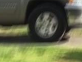
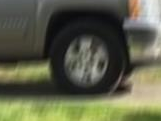
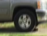
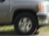
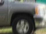
Ours
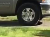
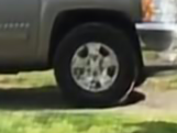
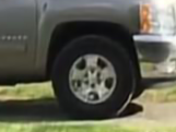
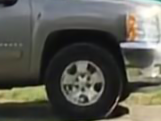
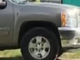
	frame $\#1$	frame $\#2$	frame $\#3$	frame $\#4$	frame $\#5$

Figure 13. Deblurring examples of a video sequence from Su et al. (2017)’s test set. Frame $\#1$ is the first frame of the input video.

B.4. Additional comparisons of pixel volume with other motion compensation approaches

In this section, we compare our pixel volume approach to two additional motion compensation approaches to analyze the effect of a pixel volume. As described in Sec. 3.2, our pixel volume approach leads to the performance improvement in video deblurring by utilizing multiple candidates with majority cues in a pixel volume. One natural question would be whether simply using the majority values in the pixel volume or multiple candidates without majority cues also leads the performance improvement. Therefore, we experimented with two other motion compensation approaches.

First, instead of our PV, we simply fed the deblurring result of the previous sharp frame warped by the majority-based warping to PVDNet. In majority-based warping, we built a PV based on the estimated flow, then chose the most frequent pixel value (the mode) among the $k^{2}$ candidates for each pixel. Second, instead of constructing our PV, we constructed a naïve PV in a way that it can provide multiple candidates without spatial coherency, corresponding to simply increase the number of candidates. Specifically, for each spatial position in a PV, we do not exploit the flow vectors of the neighbor pixels, but we simply collect pixels in the $k\times k$ window centered at the estimated position by BIMNet. This approach is similar to the neighbor search of (Cho et al., 2012) and the cost volume construction of conventional stereo matching algorithms. For the experiment and comparison, we conducted the same procedure used in Sec. 4.3.

Table 11 summarizes the performance of different approaches. The performance improvement of majority-based warping over simple warping is marginal, as the warped images from simple warping and majority-based warping would be similar to each other, as shown in Fig. 4c. The performance improvement of the naïve PV over simple warping is also marginal. Although the naïve PV contains multiple candidates, those multiple candidates do not have majority values due to the way of construction. In contrast, the multiple candidates in our PV are obtained by exploiting flow information of neighboring pixels and provide the majority cue.

Table 12. Performances with different patch sizes for a pixel volume.

Patch size	1	3	5	7	9
PSNR (dB)	31.42	31.54	31.63	31.55	31.11
SSIM	0.912	0.912	0.915	0.913	0.905

B.5. Patch size of pixel volume

In this experiment, we analyze the deblurring performance change by a different patch size of a pixel volume. We tested five patch sizes (1, 3, 5, 7, 9) and found that $5\times 5$ performs the best (Table 12). Ideally, it can be expected that a larger patch size can help the network to handle more spacious flow errors, but a large patch size rather decreases the performance in practice. This may be because a pixel volume generated by large patches contains too many candidates to consider, which exceeds the capability of PVDNet.

B.6. Pixel volume vs flow aggregation using conv layers

Our framework explicitly constructs a pixel volume for motion compensation. One natural question would be whether it would be possible to learn to aggregate flow information of neighboring pixels using additional convolution layers instead of explicit construction of a pixel volume. To verify this, we may consider the following two options:

1. Additional convolution layers at the end of BIMNet to refine the flow result

2. Additional convolution layers at the beginning of PVDNet to aggregate flow results

Specifically, the first option refines the flow result through additional convolution layers. This option is equivalent to adopt a larger network architecture for BIMNet. To verify whether this option brings a significant improvement, we trained a larger network with additional five convolution layers for BIMNet. We then measured the deblurring performance, but found no noticeable improvement.

The second option is not trivial. To deblur the current frame, video deblurring requires pixel value information of the previous frame, not its flow information (Cho et al., 2012; Su et al., 2017; Kim et al., 2017, 2018; Wang et al., 2019). Thus, even if we somehow aggregate flow information using additional convolution layers, we still need to warp the previous deblurred frame. Moreover, aggregating and refining flow information is not trivial as well. Instead, our pixel-volume approach provides an effective way that allows the network to aggregate pixel value information from multiple candidate pixels. In addition, a pixel volume takes smaller memory than a single convolution layer (Sec. 4.7).

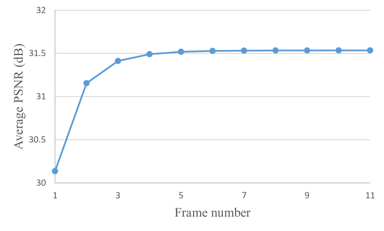
Figure 14. Performance graph of our video deblurring framework on Su et al.’s dataset (Su et al., 2017) at different time steps. The average PSNR is low at the first frame, but it quickly raises and gets stabilized as our method proceeds.

B.7. Deblurring of first few frames

Fig. 13 shows the deblurring results of the first few frames of a video. The top row shows input consecutive blurry frames, while the bottom row shows their corresponding results. When our method starts to deblur the video from the first frame, the first frame has no deblurred previous frame, and its deblurring result still has a small amount of remaining blur, e.g., the details of the wheel are slightly blurry. Nevertheless, from the second frame, our method can utilize the deblurred result of the previous frame, so it produces a clearer result with sharper details.

Fig. 14 visualizes the average PSNRs of the deblurring results at different time steps. The average PSNRs are measured from the test set of Su et al.’s dataset (Su et al., 2017). The average PSNR of the first frames is low as they have no deblurring results of the previous frames. However, as the method proceeds, the average PSNR quickly raises and gets stabilized. This proves the practicality and effectiveness of our approach despite its recurrent structure that requires deblurring results of previous frames.

References

- (1)
- Bar et al. (2007) Leah Bar, Benjamin Berkels, Martin Rumpf, and Guillermo Sapiro. 2007. A Variational Framework for Simultaneous Motion Estimation and Restoration of Motion-Blurred Video. In Proc. CVPR.
- Barnes et al. (2009) Connelly Barnes, Eli Shechtman, Adam Finkelstein, and Dan B. Goldman. 2009. PatchMatch: a randomized correspondence algorithm for structural image editing. ACM Transactions on Graphics 28, 3 (2009), 24.
- Butler et al. (2012) Daniel J. Butler, Jonas Wulff, Garrett B. Stanley, and Michael J. Black. 2012. A naturalistic open source movie for optical flow evaluation. In Proc. ECCV.
- Cho and Lee (2009) Sunghyun Cho and Seungyong Lee. 2009. Fast Motion Deblurring. ACM Transactions on Graphics 28, 5, Article 145 (2009), 145:1–145:8 pages.
- Cho et al. (2012) Sunghyun Cho, Jue Wang, and Seungyong Lee. 2012. Video Deblurring for Hand-held Cameras Using Patch-based Synthesis. ACM Transactions on Graphics 31, 4, Article 64 (2012), 64:1–64:9 pages.
- Daraei (2014) Mohammad Hossein Daraei. 2014. Optical Flow Computation in the Presence of Spatially-Varying Motion Blur. In Proc. ISVC.
- Delbracio and Sapiro (2015a) Mauricio Delbracio and Guillermo Sapiro. 2015a. Burst deblurring: Removing camera shake through fourier burst accumulation. In Proc. CVPR.
- Delbracio and Sapiro (2015b) Mauricio Delbracio and Guillermo Sapiro. 2015b. Hand-Held Video Deblurring Via Efficient Fourier Aggregation. IEEE Transactions on Computational Imaging 1, 4 (2015), 270–283.
- Dosovitskiy et al. (2015) Alexey Dosovitskiy, Philipp Fischer, Eddy Ilg, Philip Häusser, Caner Hazırbaş, Vladimir Golkov, Patrick v.d. Smagt, Daniel Cremers, and Thomas Brox. 2015. FlowNet: Learning Optical Flow with Convolutional Networks. In Proc. ICCV.
- Gast and Roth (2019) Jochen Gast and Stefan Roth. 2019. Deep Video Deblurring: The Devil is in the Details. In Proc. ICCVW.
- Ge et al. (2018) Weifeng Ge, Bingchen Gong, and Yizhou Yu. 2018. Image Super-Resolution via Deterministic-Stochastic Synthesis and Local Statistical Rectification. ACM Transactions on Graphics 37, 6, Article 260 (2018), 14 pages.
- Geiger et al. (2012) Andreas Geiger, Philip Lenz, and Raquel Urtasun. 2012. Are we ready for Autonomous Driving? The KITTI Vision Benchmark Suite. In Proc. CVPR.
- He et al. (2017) K. He, G. Gkioxari, P. Dollár, and R. Girshick. 2017. Mask R-CNN. In Proc. ICCV.
- Hirsch et al. (2011) Michael Hirsch, Christian J. Schuler, Stefan Harmeling, and Bernhard Schölkopf. 2011. Fast removal of non-uniform camera shake. In Proc. ICCV.
- Hui et al. (2018) Tak-Wai Hui, Xiaoou Tang, and Chen Change Loy. 2018. LiteFlowNet: A Lightweight Convolutional Neural Network for Optical Flow Estimation. In Proc. CVPR.
- Ilg et al. (2017) Eddy Ilg, Nikolaus Mayer, Tonmoy Saikia, Margret Keuper, Alexey Dosovitskiy, and Thomas Brox. 2017. FlowNet 2.0: Evolution of Optical Flow Estimation with Deep Networks. In Proc. CVPR.
- Jaderberg et al. (2015) Max Jaderberg, Karen Simonyan, Andrew Zisserman, and koray kavukcuoglu. 2015. Spatial Transformer Networks. In Proc. NIPS.
- Kim et al. (2013) Tae Hyun Kim, Byeongjoo Ahn, and Kyoung Mu Lee. 2013. Dynamic Scene Deblurring. In Proc. ICCV.
- Kim and Lee (2015) Tae Hyun Kim and Kyoung Mu Lee. 2015. Generalized video deblurring for dynamic scenes. In Proc. CVPR.
- Kim et al. (2017) Tae Hyun Kim, Kyoung Mu Lee, Bernhard Schölkopf, and Michael Hirsch. 2017. Online Video Deblurring via Dynamic Temporal Blending Network. In Proc. ICCV.
- Kim et al. (2018) Tae Hyun Kim, Mehdi S. M. Sajjadi, Michael Hirsch, and Bernhard Scholkopf. 2018. Spatio-temporal Transformer Network for Video Restoration. In Proc. ECCV.
- Kingma and Ba (2015) Diederik Kingma and Jimmy Ba. 2015. Adam: A Method for Stochastic Optimization. In Proc. ICLR.
- Köhler et al. (2012) Rolf Köhler, Michael Hirsch, Betty Mohler, Bernhard Schölkopf, and Stefan” Harmeling. 2012. Recording and Playback of Camera Shake: Benchmarking Blind Deconvolution with a Real-World Database. In Proc. ECCV.
- Kupyn et al. (2018) Orest Kupyn, Volodymyr Budzan, Mykola Mykhailych, Dmytro Mishkin, and Jiri Matas. 2018. DeblurGAN: Blind Motion Deblurring Using Conditional Adversarial Networks. In Proc. CVPR.
- Lee and Lee (2013) Hee Seok Lee and Kyoung Mu Lee. 2013. Dense 3D Reconstruction from Severely Blurred Images Using a Single Moving Camera. In Proc. CVPR.
- Liao et al. (2015) R. Liao, X. Tao, R. Li, Z. Ma, and J. Jia. 2015. Video Super-Resolution via Deep Draft-Ensemble Learning. In Proc. ICCV.
- Loshchilov and Hutter (2017) Ilya Loshchilov and Frank Hutter. 2017. SGDR: Stochastic Gradient Descent with Restarts. In Proc. ICLR.
- Matsushita et al. (2006) Yasuyuki Matsushita, Eyal Ofek, Weina Ge, Xiaoou Tang, and Heung Yeung Shum. 2006. Full-frame video stabilization with motion inpainting. IEEE Transactions on Pattern Analysis and Machine Intelligence 28, 7 (2006), 1150–1163.
- Mayer et al. (2016) Nikolaus Mayer, Eddy Ilg, Philip Häusser, Philipp Fischer, Daniel Cremers, Alexey Dosovitskiy, and Thomas Brox. 2016. A Large Dataset to Train Convolutional Networks for Disparity, Optical Flow, and Scene Flow Estimation. In Proc. CVPR.
- Nah et al. (2017) Seungjun Nah, Tae Hyun Kim, and Kyoung Mu Lee. 2017. Deep Multi-Scale Convolutional Neural Network for Dynamic Scene Deblurring. In Proc. CVPR.
- Nah et al. (2019) Seungjun Nah, Sanghyun Son, and Kyoung Mu Lee. 2019. Recurrent Neural Networks With Intra-Frame Iterations for Video Deblurring. In Proc. CVPR.
- Pan et al. (2016) Jinshan Pan, Zhe Hu, Zhixun Su, Hsin-Ying Lee, and Ming-Hsuan Yang. 2016. Soft-Segmentation Guided Object Motion Deblurring. In Proc. CVPR.
- Portz et al. (2012) Travis Portz, Li Zhang, and Hongrui Jiang. 2012. Optical flow in the presence of spatially-varying motion blur. In Proc. CVPR.
- Ren et al. (2015) Shaoqing Ren, Kaiming He, Ross B. Girshick, and Jian Sun. 2015. Faster R-CNN: Towards Real-Time Object Detection with Region Proposal Networks.. In Proc. NIPS.
- Ren et al. (2017) Wenqi Ren, Jinshan Pan, Xiaochun Cao, and Ming-Hsuan Yang. 2017. Video Deblurring via Semantic Segmentation and Pixel-Wise Non-Linear Kernel. In Proc. ICCV.
- Ren et al. (2019) Yurui Ren, Xiaoming Yu, Ruonan Zhang, Thomas H. Li, Shan Liu, and Ge Li. 2019. StructureFlow: Image Inpainting via Structure-aware Appearance Flow. In Proc. ICCV.
- Ronneberger et al. (2015) Olaf Ronneberger, Philipp Fischer, and Thomas Brox. 2015. U-Net: Convolutional Networks for Biomedical Image Segmentation. In Proc. MICCAI.
- Scharstein et al. (2014) Daniel Scharstein, Heiko Hirschmüller, York Kitajima, Greg Krathwohl, Nera Nesic, Xi Wang, and Porter Westling. 2014. High-Resolution Stereo Datasets with Subpixel-Accurate Ground Truth.. In Proc. GCPR.
- Seibold et al. (2017) Clemens Seibold, Anna Hilsmann, and Peter Eisert. 2017. Model-based motion blur estimation for the improvement of motion tracking. Computer Vision and Image Understanding 160 (2017), 45 – 56.
- Su et al. (2017) Shuochen Su, Mauricio Delbracio, Jue Wang, Guillermo Sapiro, Wolfgang Heidrich, and Oliver Wang. 2017. Deep Video Deblurring for Hand-held Cameras. In Proc. CVPR.
- Sun et al. (2018) Deqing Sun, Xiaodong Yang, Ming-Yu Liu, and Jan Kautz. 2018. PWC-Net: CNNs for Optical Flow Using Pyramid, Warping, and Cost Volume. In Proc. CVPR.
- Sánchez et al. (2013) Javier Sánchez, Enric Meinhardt-Llopis, and Gabriele Facciolo. 2013. TV-L1 Optical Flow Estimation. Image Processing On Line 3 (2013), 137–150.
- Tao et al. (2018) Xin Tao, Hongyun Gao, Xiaoyong Shen, Jue Wang, and Jiaya Jia. 2018. Scale-recurrent Network for Deep Image Deblurring. In Proc. CVPR.
- Wang et al. (2019) Xintao Wang, Kelvin C.K. Chan, Ke Yu, Chao Dong, and Chen Change Loy. 2019. EDVR: Video Restoration with Enhanced Deformable Convolutional Networks. In Proc. CVPRW.
- Wang et al. (2004) Zhou Wang, Alan C. Bovik, Hamid R. Sheikh, and Eero P. Simoncelli. 2004. Image quality assessment: from error visibility to structural similarity. IEEE Transactions on Image Processing 13, 4 (2004), 600–612.
- Whyte et al. (2012) Oliver Whyte, Josef Sivic, Andrew Zisserman, and Jean Ponce. 2012. Non-uniform Deblurring for Shaken Images. International Journal of Computer Vision 98, 2 (2012), 168–186.
- Wulff and Black (2014) Jonas Wulff and Michael J. Black. 2014. Modeling Blurred Video with Layers. In Proc. ECCV.
- Xu and Jia (2010) Li Xu and Jiaya Jia. 2010. Two-Phase Kernel Estimation for Robust Motion Deblurring. In Proc. ECCV.
- Xu and Jia (2012) Li Xu and Jiaya Jia. 2012. Depth-Aware Motion Deblurring. In Proc. ICCP.