Thermodynamic uncertainty relations for many-body systems with fast jump rates and large occupancies

Abstract

A universal large $\mathcal{N}$ theory of nonequilibrium fluctuations emerges in the limit of fast jump rates and large occupancies. We use this theory to derive a set of coarse grained thermodynamic uncertainty relations (TUR) – one of them being an activity bound. Importantly, the activity serves as a tighter bound for the entropy production in 1D systems. These results are particularly useful in the many-body regime, where typically a coarse grained approach is required to handle the large microscopic state space.

I Introduction

The second law of thermodynamics resulting in, e.g. the Carnot bound on the maximum efficiency of thermal engines, demonstrates the importance that inequalities play in physics. The Carnot efficiency bound is remarkably independent of specific design. More recently and in the same spirit, the thermodynamic uncertainty relations (TUR) Barato and Seifert (2015); Gingrich et al. (2016); Horowitz and Gingrich (2020) revealed that fluctuations in thermal systems cannot be freely minimised. Rather they are bounded from below by the inverse entropy production irrespective of system design. The ideas of the TUR led to an effort towards optimizing the bounds Pal et al. (2021a); Macieszczak et al. (2018); Shiraishi (2020); Pal et al. (2021b), generalizing the bound in the regime of large deviations Fischer et al. (2018); Gingrich and Horowitz (2017), quantum systems Hasegawa (2021); Miller et al. (2021); Hasegawa (2020); Liu and Segal (2019), explicit time-dependence Horowitz and Gingrich (2017), athermal analogues Soret et al. (2020) and results of the same spirit Shiraishi et al. (2018); Falasco et al. (2020); Polettini et al. (2021); Shpielberg and Nemoto (2019); Manikandan and Krishnamurthy (2018).

A common starting point for discussing the TUR is via a master equation. The master matrix of the rates may be time-dependent or not. This language is particularly suited for a single particle dynamics, where a state corresponds to the particle localised in a given site. For many body systems, the applicability of the TUR is limited due to the large state space. Namely, evaluating the particle densities involves finding the zero eigenvalue state of a large Markov matrix. Similarly, evaluating current fluctuations requires finding the largest eigenvalue of a large tilted Markov matrix Derrida et al. (2004) (also see detailed discussion later). This renders the overall procedure tedious and quite often intractable.

Indeed, it is only in $1D$ non-equilibrium steady state that the current and current fluctuations are evaluated along a single bond only. But for any generic network, accounting for a large number of states, calculating, measuring or obtaining numerically the fluctuations of the current is typically hard: thus limiting the usefulness of the TUR and its large deviation bound counterpart. This difficulty can be overcome using universal non-equilibrium theories that result in a coarse grained picture, allowing a compact description to calculate current statistics Bertini et al. (2015); Maes and Netočný (2008); Monthus (2019); Spohn (2014); Meerson and Smith (2019). Naturally, the question arises on whether one can write a useful TUR in a coarse grained manner.

In this work, we show how this can be done in a systematic way from a nonequilibrium theory: Consider a master equation with fast rates and large particle occupancies on a finite graph Gabrielli and Renger (2020); Baek et al. (2016). The fast-rates-large-occupancy large $\mathcal{N}$ limit leads to a universal coarse grained non-equilibrium theory, dubbed here – the large $\mathcal{N}$ theory (see also Monthus (2019)). Within the framework of this large $\mathcal{N}$ theory, we show that the variance of the current is bounded from below by either the activities or the coarse grained entropy production. Interestingly, the activity serves as an upper bound for the entropy production and a tighter bound in $1D$ systems. The latter bound becomes tight in the large $\mathcal{N}$ limit hence serving as a better tool to infer entropy production. These results, reinstate the importance and relevance of the TUR and similar inequalities in many body systems even in the case where the states space is unmanageable to treat, analytically or numerically.

The outline of this work is as follows. In Sec. II, we lay the setup for the large $\mathcal{N}$ theory and present the main results. In Sec. III, we numerically validate the main results for a particular interacting model system: the asymmetric inclusion process (ASIP) at finite $\mathcal{N}$ Reuveni et al. (2012); Grosskinsky et al. (2011). Sec. IV focuses on the derivation of the bound and the results of Sec. II. We conclude in Sec. V where we summarise the work and point out future directions.

II Setup and results

Consider a stochastic process with a finite set of sites with particle occupancies $n_{x}=0,1,2,...$. Assume that a particle jumps from site $x$ to $y$ with rate $\tilde{\kappa}_{y,x}$ that may depend on the local occupancies. Particles are added to / removed from the system only through a finite number of bonds to a reservoir or a set of reservoirs. In particular, we restrict the discussion to processes with fast rates; scaling like $\mathcal{N}^{2}$ with respect to the large parameter $\mathcal{N}\gg 1$. Under this assumption, we consider the rescaled occupancies $\rho_{x}(\tau)=n_{x}/\mathcal{N}$ and the rescaled time $\tau=\mathcal{N}t$. Then, $\tilde{\kappa}_{y,x}=\mathcal{N}^{2}\kappa_{y,x}+O(\mathcal{N})$, where $\kappa_{y,x}$ depends only on the rescaled densities $\rho$. Gathering these definitions, the rescaled evolution equation is

$$\partial_{\tau}\rho_{x} = -(\mathrm{div}\,\kappa)_{x},$$ (1)

$$(\mathrm{div}\,\kappa)_{x} = -\sum_{y\sim x}\kappa_{x,y}-\kappa_{y,x},$$

where $\sum_{y\sim x}$ denotes summation over all the neighbors of $x$. Note that this summation may include the coupling to reservoirs which are assumed to have fixed densities. We now define the empirical unidirectional flux $\tilde{q}_{x,y}(t)$ that counts the number of particles jumping from site $y$ to $x$ during the time interval $\left[t,t+dt\right]$. At the large $\mathcal{N}$ limit, the rescaled empirical unidirectional flux is $\tilde{q}_{y,x}(t)=\mathcal{N}^{2}q_{y,x}(\tau)+O(\mathcal{N})$. Note that, on average, $\langle q_{x,y}(\tau)\rangle=\langle\kappa_{x,y}(\rho(\tau))\rangle=\kappa_{x,y}(\langle\rho(\tau)\rangle)$. The last equality uses the mean field approximation, which will be shown to be exact at $\mathcal{N}\rightarrow\infty$. The notation $\kappa(\rho)$ implies that $\kappa$ depends on the local densities. The (rescaled) empirical current is given by $j_{x,y}(\tau)\equiv q_{x,y}(\tau)-q_{y,x}(\tau)$. We further define $J_{y,x}(\rho)\equiv\kappa_{y,x}-\kappa_{x,y}$. Thus, on average, $\langle j_{y,x}\rangle=\langle J_{y,x}(\rho)\rangle=J_{y,x}(\langle\rho\rangle)$ and again the last inequality is exact only in the limit $\mathcal{N}\rightarrow\infty$. Lastly, we define the local activity $a_{x,y}\equiv q_{x,y}+q_{y,x}$ Maes and Netočný (2008) that will play an important role later on.

In what follows, we explore the properties of a generalized fluctuating charge transfer defined in the following

$$Q=\mathcal{N}\int^{\tau}_{0}d\tau^{\prime}\,\sum_{x}\sum_{y>x}d_{y,x}j_{y,x}+\sum_{x}u_{x}\rho_{x},$$ (2)

where $d_{y,x},u_{x}$ are predetermined weights. We furthermore define $d_{x,y}=-d_{y,x}$ for convenience. It has no bearing on $Q$. Note that the functional contains both the current and occupation like terms. In this work, we derive a bound for the cumulant generating function $\mu(\lambda)\equiv\frac{1}{\mathcal{N}\tau}\ln\langle e^{\lambda Q}\rangle$ of the charge $Q$ at the steady state. In particular, the bound on the generalized current variance reads

$$\mu^{\prime\prime}(0) \geq (d^{\perp})^{2}\langle A^{\parallel}\rangle,$$ (3)

where $(A^{\parallel})^{-1}\equiv\sum_{x,y>x}\frac{1}{a_{y,x}}$ – an impedance-like parallel summation over the activities, and $d^{\perp}\equiv\sum_{x,y>x}d_{y,x}$ – an impedance-like series summation over the weights. Detailed derivation of our results is presented in Sec. IV. In the large $\mathcal{N}$ theory, $\langle a^{-1}_{x,y}\rangle=\langle a_{x,y}\rangle^{-1}$ and the mean bond activities depends only on the mean densities. The lower bound is accessible analytically and numerically. Moreover, even if the rates are not known, the activities – a measure on the number of jumps – are still accessible experimentally in many cases Iwase et al. (2013); Svetlizky and Roichman (2021). Interestingly, the activity bound (3) can further be generalized to a large deviation bound (14) that we show later.

In particular for a 1D lattice, we can improve the well known entropy production bound by using the parallel activity

$$\mu^{\prime\prime}(0) \geq (d^{\perp})^{2}\langle A^{\parallel}\rangle\geq\frac{2(\mu^{\prime}_{j})^{2}}{\langle\Sigma\rangle},$$ (4)

with $\mu^{\prime}_{j}\equiv\sum_{x,y>x}d_{y,x}\langle j_{y,x}\rangle$ and

$$\Sigma=\sum_{x,y>x}j_{y,x}\log\frac{a_{y,x}+j_{y,x}}{a_{y,x}-j_{y,x}},$$ (5)

as the entropy production rate Seifert (2012); Van den Broeck and Esposito (2015). A similar series of bounds as in (4) was already derived in the case of a 1D periodic system governed by a master equation Barato et al. (2018). Notice that Barato et al. (2018) was evaluated through the microscopic master equation itself whereas in our case, we are interested in the coarse grained quantities, e.g. the densities $\rho$ and the rescaled rates $\kappa$. Therefore, the coarse grained series of inequalities need not be exact at finite $\mathcal{N}$ and deviations from it are observed, but controlled. See Fig.1. As noted before, (4) suggests the bound is given in terms of the mean local activities which are accessible numerically, analytically and usually also experimentally when dealing with a finite graph.

Lastly, let us use (4) to imply two more appealing bounds. Notice that $A^{\parallel}\leq A^{\perp}/(\sum_{x,y>x}1)^{2}$ by Titu’s lemma Sedrakyan and Sedrakyan (2018) where $A^{\perp}$ is the activity series summation. Furthermore, $A^{\parallel}\leq a_{x,y}$ for any bond pair $x,y$. This leads to two bounds

$$\langle\Sigma\rangle \geq\frac{2(\mu^{\prime}_{j})^{2}(\sum_{x,y>x}1)^{2}}{(d^{\perp})^{2}\langle A^{\perp}\rangle},$$ (6)

$$\langle\Sigma\rangle \geq\frac{2(\mu^{\prime}_{j})^{2}}{(d^{\perp})^{2}\langle a_{x,y}\rangle}\quad\forall x,y.$$ (7)

The first bound limits the entropy production in terms of the activity. This bound does not bear the same content as the kinetic uncertainty relation Di Terlizzi and Baiesi (2019) as it bounds the entropy production and not the current variance. The second inequality is particularly interesting for practical purposes. It allows to get a lower bound on the entropy production from a single bond current and activity. In 1D systems, the steady state current is uniform for any bond i.e. $\mu^{\prime}_{j}=d^{\perp}\langle j_{y,x}\rangle,\forall\,y>x$. The activity, however, is not uniform which makes this result surprising.

III Application: the ASIP

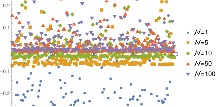
(a) $200$ realizations of the ASIP with random rates $p_{\pm}(x)\in\left[0,1\right]$ where $N=2$ particles and $L=3$ sites with periodic boundary conditions.

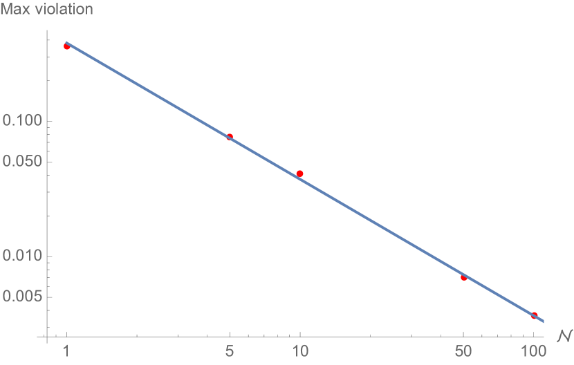
(b) The negative of minimal values of $\frac{\mu^{\prime\prime}(0)-(d^{\perp})^{2}\langle A^{\parallel}\rangle}{\mu^{\prime\prime}(0)}$ out of all the random realizations for each $\mathcal{N}$ – the max violation.

Figure 1: Numerical demonstration of the first inequality in (4). The value of $\frac{\mu^{\prime\prime}(0)-(d^{\perp})^{2}\langle A^{\parallel}\rangle}{\mu^{\prime\prime}(0)}$ in the random ASIP. We present $200$ random realizations for each $\mathcal{N}$ value. (a) The minimal values of the random realizations are seen to converge to zero with increasing $\mathcal{N}$. (b) The violation – the negative of the minimal value of all the realizations – is shown to vanish like $1/\mathcal{N}$, as expected from the large $\mathcal{N}$ theory. The fitting gives a slope of $-1.008$ close to the expected slope of $-1$ at $\mathcal{N}=\infty$. For more details, see Sec. C.

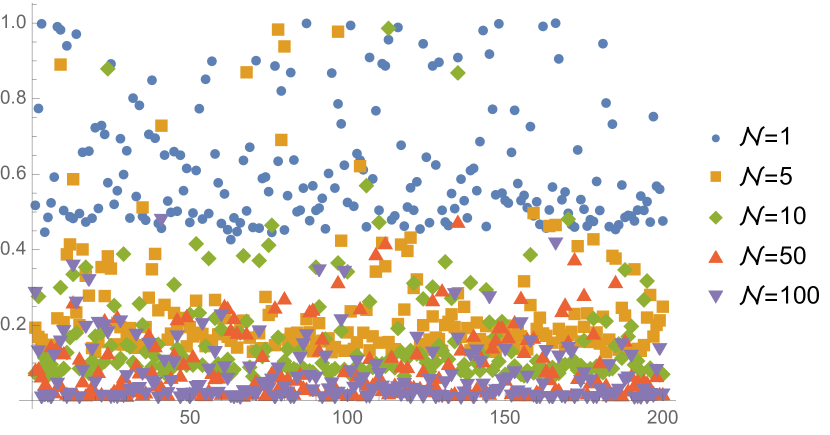
(a) $200$ realizations of the ASIP with random rates $p_{\pm}(x)\in\left[0,1\right]$ where $N=2$ particles and $L=3$ sites with periodic boundary conditions.

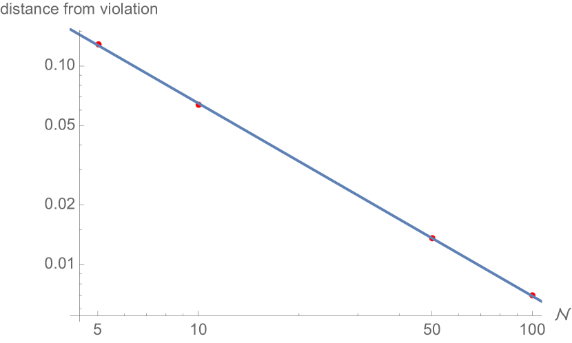
(b) The minimal value of $\frac{(d^{\perp})^{2}\langle A^{\parallel}\rangle-2(\mu^{\prime}_{j})^{2}/\langle\Sigma\rangle}{(d^{\perp})^{2}\langle A^{\parallel}\rangle}$ out of all the random realizations for each $\mathcal{N}$. Here, this is the distance from violation of the bound.

Figure 2: Numerical demonstration of the second inequality in (4). The evidence of $\frac{(d^{\perp})^{2}\langle A^{\parallel}\rangle-2(\mu^{\prime}_{j})^{2}/\langle\Sigma\rangle}{(d^{\perp})^{2}\langle A^{\parallel}\rangle}\geq 0$ in the random ASIP. We present $200$ random realizations for each $\mathcal{N}$ value. (a) The minimal values of the random realizations are seen to converge to zero with increasing $\mathcal{N}$ indicating the tightening of the bound. (b) The distance from violation – the minimal value of all the realizations – is shown to vanish like $1/\mathcal{N}$. The fitting gives a slope of $-0.9715$ close to the expected slope of $-1$ at $\mathcal{N}=\infty$. For more details, see Sec. C.

In this section, we illustrate our results using an interacting particle system namely the Asymmetric Inclusion Process (ASIP) Reuveni et al. (2012); Grosskinsky et al. (2011). In particular, we focus on the dynamics on a 1D chain Reuveni et al. (2012); Grosskinsky et al. (2011) where we have $\tilde{\kappa}_{x\pm 1,x}=p_{\pm}(x)n_{x}(\mathcal{N}+n_{x\pm 1})$ with the rates $p_{\pm}(x)\geq 0$. Then, $\kappa_{x\pm 1,x}=p_{\pm}(x)\rho_{x}(1+\rho_{x+1})$. To validate our claims, in particular (4), we consider the ASIP with $N=2$ particles and a periodic system of $L=3$ sites and random rates $p_{\pm}(x)\in[0,1]$. We evaluate the local densities at the steady state and recover local coarse grained activities and currents.

In Fig.1, the inequality $\mu^{\prime\prime}(0)-(d^{\perp})^{2}\langle A^{\parallel}\rangle\geq 0$ is demonstrated in the large $\mathcal{N}$ limit, with $1/\mathcal{N}$ corrections, as expected from the large $\mathcal{N}$ theory. Namely, the inequality is precise only at $\mathcal{N}\rightarrow\infty$. In Fig. 2, the inequality $(d^{\perp})^{2}\langle A^{\parallel}\rangle\geq 2(\mu^{\prime}_{j})^{2}/\langle\Sigma\rangle$ is shown to hold for any $\mathcal{N}$. This need not be generally true, and probably results from the particular choice of the ASIP dynamics. Nevertheless, this inequality is shown to become the tightest in the large $\mathcal{N}$ limit with $1/\mathcal{N}$ convergence. Further details on the numerical results are discussed in the Appendices C and D.

IV Derivation of the bounds

In this section, we derive the central results that were highlighted in Sec. II. We start by noting that the joint path probability for the current and density at the large $\mathcal{N}$ limit is given by $P(j,\rho)\sim\exp{(-\mathcal{N}\int d\tau\mathcal{L})}$ Monthus (2019) (also, see the appendix A and the discussion ). The Lagrangian $\mathcal{L}$ defines the path probability at the large $\mathcal{N}$ limit up to $1/\mathcal{N}$ corrections with

$$\mathcal{L}=\sum_{x,y>x}\Phi(j_{y,x},\kappa_{y,x},\kappa_{x,y}),$$ (8)

where

$$\Phi\left(j,\kappa_{+},\kappa_{-}\right) = j\ln{\frac{j+\sqrt{j^{2}+4\kappa_{+}\kappa_{-}}}{2\kappa_{+}}}$$

$$-\sqrt{j^{2}+4\kappa_{+}\kappa_{-}}+\kappa_{+}+\kappa_{-}.$$

Note that the summation in (8) avoids double counting of the bonds. The expression (IV) is not new, and can be found in Monthus (2019); Gabrielli and Renger (2020); Baek et al. (2016) and of course earlier in the non-interacting limits where $\kappa_{y,x}\propto\rho_{x}$ Maes and Netočný (2008). Note that $\mathcal{L}$ is not limited to closed systems. In open systems, the incoming/outgoing rates $\kappa_{\pm}$ may depend on the fixed density of the reservoirs Baek et al. (2016); Monthus (2019). In this case, the state space of the Markov matrix is unbounded and the large $\mathcal{N}$ theory is particularly useful.

It is now useful to present the Lagrangian $\mathcal{L}_{Y}$, which depends on the tilting field $Y_{y,x}$, constrained to satisfy Kirchhoff’s junction rule Dechant and Sasa (2018); Soret et al. (2020)

$$\sum_{y\sim x}Y_{y,x}=0~{}~{}\text{and}~{}~{}Y_{y,x}=-Y_{x,y}.$$ (10)

The expression is defined locally $\Phi_{Y}(j,\kappa_{+},\kappa_{-})\equiv\Phi(j,\kappa_{+}+\frac{1}{2}Y,\kappa_{-}-\frac{1}{2}Y)$ which leads to the steady state densities $\langle\rho_{x}\rangle=\langle\rho_{x}\rangle_{Y}$, but a different steady state current $\langle j_{y,x}\rangle_{Y}=\langle j_{y,x}\rangle+Y_{y,x}$ . The averaging $\langle\,\cdot\,\rangle_{Y}$ is with respect to the tilted Lagrangian $\mathcal{L}_{Y}$. One natural choice for the tilted dynamics is to induce a mapping to equilibrium, i.e. setting $\langle j_{x,y}\rangle_{Y}=0$, implying the choice $Y_{y,x}=-\langle j_{y,x}\rangle=\langle\kappa_{x,y}-\kappa_{y,x}\rangle$. Another natural choice is to set $Y$ such that $\langle j_{x,y}\rangle_{Y}=-\langle j_{x,y}\rangle$, realizing the steady state time-reversed dynamics. This in turn allows one to evaluate the entropy production – a central quantity in the study of non-equilibrium physics. Recently, Dechant and Sasa also used a similar idea to extend the time reversal mapping in order to possibly tighten the TUR Dechant and Sasa (2020).

Here, the tilted dynamics allows more freedom, but in turn may lose an amenable physical interpretation as $\Phi$ is defined only for non-negative $\kappa_{+}$. Nevertheless, this mathematical trick leads to an optimized bound with a clear physical interpretation. Moreover, it allows us to optimizes the bound on the variance of $Q$ via a set of linear equations (see (16)).

The cumulant generating function can now be expressed using the tilted dynamics

$$\mu(\lambda)=\frac{1}{\mathcal{N}\tau}\log\langle e^{\lambda Q+\mathcal{N}\int d\tau\,\mathcal{L}_{Y}-\mathcal{L}}\rangle_{Y}.$$ (11)

Using the Jensen inequality in above leads to

$$\mu(\lambda)\geq\frac{\lambda}{\mathcal{N}\tau}\langle Q\rangle_{Y}+\langle\mathcal{L}_{Y}-\mathcal{L}_{0}\rangle_{Y}.$$ (12)

Note that at this point, optimization of (12) with respect to the tilting field $Y$ leads to a set of non-linear equations which are hard to solve in general. To produce a useful inequality on the current fluctuations, we take (12) together with the rescaling $Y\rightarrow\lambda Y$ Dechant and Sasa (2020) and expand both sides to second order in $\lambda$

$$\frac{1}{2}\mu^{\prime\prime}(0)\geq\sum_{x,y>x}d_{y,x}Y_{y,x}-Y^{2}_{y,x}\frac{1}{2\langle a_{y,x}\rangle}.$$ (13)

Recall that $a_{y,x}=\kappa_{x,y}(\rho)+\kappa_{y,x}(\rho)$ is the bond activity. Eq.(13) together with Kirchhoff’s junction rule (10) compose one of the central results of this work. We stress that the explicit result could be obtained due to the the saddle point approximation in the path probability resulting from the large $\mathcal{N}$ value. For finite $\mathcal{N}$, (13) and what follows from it, may be erroneous as demonstrated for finite $\mathcal{N}$ in Fig. 1. Taken together with the Kirchhoff’s junction rule (10) – which is a constraint, and simultaneous minimization of $Y_{x,y}$ leads to tightening the TUR.

Eq.(13) implies that many different bounds could be obtained. In what follows we discuss two particular choices for $Y$ leading to two different bounds: the activity bound and the entropy production bound. Then we discuss how to optimize the bound using the tilting field. We conclude this section by showing that for 1D systems, the bounds can be ordered, making them particularly useful. For completeness, we also connect our derivation to the kinetic uncertainty bound Di Terlizzi and Baiesi (2019); Shiraishi (2020); Pal et al. (2021a) in the Appendix E.

IV.1 Activity bound

Let us first explore the simplest tilting field $Y_{y,x}=Y$ for $y>x$ together with $Y_{y,x}=-Y_{x,y}$ satisfying Kirchhoff’s rule (10). The resulting bound is still valid for any $Y$. Optimization of the constant $Y$ (see the right hand side of Eq.(13)) leads to $Y=d^{\perp}\langle A^{\parallel}\rangle$ and to the activity bound (3). Furthermore, we can directly use this (suboptimal) choice of $Y$ in (12), leading to the large deviation bound

$$\mu(\lambda)-\lambda\mu^{\prime}(0)\geq(d^{\perp})^{2}\lambda^{2}\langle A^{\parallel}\rangle-\langle\mathcal{L}_{0}\rangle_{\lambda d^{\perp}\langle A^{\parallel}\rangle}.$$ (14)

While the right hand side of (14) seems cumbersome, it can be evaluated in a straight-forward manner using the mean local activities and currents only or through the densities if the rates $\kappa$ are known.

IV.2 Optimizing the bound

Next, we sketch the optimization of the bound with respect to the tilting field. Define $F_{Y}$ such that $\mu^{\prime\prime}(0)\geq 2F_{Y}$ according to (13) and Kirchhoff’s junction rule (10). Then, we aim to find the maximum of

$$F_{Y}=\sum_{x,y>x}\left(d_{y,x}Y_{y,x}-\frac{Y^{2}_{y,x}}{2\langle a_{y,x}\rangle}\right)+\nu_{x}\sum_{y\sim x}Y_{y,x}$$ (15)

where $\nu_{x}$ are Lagrange multipliers accounting for Kirchhoff’s junction rule (10). The solution to this optimization problem is

$$2F_{Y,\mathrm{max}} =\sum_{x,y>x}d^{2}_{y,x}\langle a_{y,x}\rangle-\langle a_{y,x}\rangle^{2}(\nu_{x}-\nu_{y})^{2},$$

$$0 =\sum_{y\sim x}(d_{y,x}+\nu_{x}-\nu_{y})\langle a_{y,x}\rangle.$$ (16)

Note that one needs to first solve the set of linear equations (16) to obtain $F_{Y,\text{max}}$. The size of the set is essentially the number of bonds in the graph while coupling to reservoirs enlarges this number. A different optimization scheme was carried out recently resulting in the same optimized bound Shiraishi (2020). Other useful bounds can be obtained from (13). In what follows, we present a few physically relevant bounds and explore their relation and relevance.

IV.3 Relations between bounds

In this subsection, we benchmark the TURs which were derived in Barato et al. (2018); Gingrich et al. (2016), using the tilted $Y$ approach. Consider $Y_{y,x}=\alpha\langle j_{y,x}\rangle$. This choice satisfies the Kirchhoff’s rule for any constant $\alpha$ as the steady state current is divergence free. Furthermore, one can show that $2\frac{\langle j_{y,x}\rangle^{2}}{\langle a_{y,x}\rangle}\leq j_{y,x}\log\frac{\langle a_{x,y}\rangle+\langle j_{x,y}\rangle}{\langle a_{x,y}\rangle-\langle j_{x,y}\rangle}$ as $2x^{2}\leq x\log\frac{1+x}{1-x}$ for $x=\frac{j}{a}\in\left[-1,1\right]$. Simple additivity of terms imply then $\sum_{y>x}2\frac{\langle j_{x,y}\rangle^{2}}{\langle a_{x,y}\rangle}\leq\langle\Sigma\rangle$. Hence we recover $\mu^{\prime\prime}(0)\geq\alpha\mu^{\prime}_{j}-\frac{\alpha^{2}}{4}\langle\Sigma\rangle$. Finding the optimal $\alpha$ leads to the entropy production bound

$$\mu(\lambda)-\lambda\mu^{\prime}(0) \geq\frac{\lambda^{2}}{2}\frac{2(\mu^{\prime}_{j})^{2}}{\langle\Sigma\rangle},$$ (17)

$$\mu^{\prime\prime}(0) \geq\frac{2(\mu^{\prime}_{j})^{2}}{\langle\Sigma\rangle}.$$ (18)

The entropy production bound as well as the activity bound can be derived by a certain choice of the tilting field $Y_{x,y}$. Therefore, it is not only the current variance that can serve as an upper bound. Let us define $\mathcal{F}\equiv\sum_{x,y>x}d^{2}_{y,x}\langle a_{y,x}\rangle$, namely it optimizes the tilting field $Y_{x,y}$ without necessarily satisfying Kirchhoff’s rule (10). Therefore, we find that

$$\mathcal{F}\geq 2\frac{(\mu^{\prime}_{j})^{2}}{\langle\Sigma\rangle},(d^{\perp})^{2}\langle A^{\parallel}\rangle.$$ (19)

Eq.(19) could be made more physically relevant. The non-negativity of $d^{2}_{y,x},\langle a_{y,x}\rangle$ implies $\mathcal{F}\leq\sum_{y>x}d^{2}_{y,x}\langle A^{\perp}\rangle$. Therefore, we recover from (19) the physical bound

$$\sum_{y>x}d^{2}_{y,x}\langle A^{\perp}\rangle\geq 2\frac{(\mu^{\prime}_{j})^{2}}{\langle\Sigma\rangle}.$$ (20)

It is important to notice that (20) is valid for any graph, unlike (6) which are valid for the case of a $1D$ chain.

At this point, it is unclear whether $\mathcal{F}$ relates to either $\mu(\lambda)-\lambda\mu^{\prime}(0)$, $\mu^{\prime\prime}(0)$. In what follows, we discuss a special case where one can order the bounds as already noticed in Barato et al. (2018). Furthermore, we show that $\mathcal{F}$ and $\mu^{\prime\prime}(0)$ do not bound one another.

IV.4 Application of TUR in 1D lattice – A series of bounds

Consider an 1D lattice of $L$ sites which can be either open (boundary driven) or with periodic boundary conditions. Other boundary conditions can also be treated. We furthermore assume only nearest neighbors jumps . In this case, there is a single solution to Kirchhoff’s junction rule (10): $Y\equiv Y_{x+1,x}$ for any $x$ on the lattice. This in turn implies that the bound (3) is indeed optimal in the $1D$ setup. Notice that the summation depends on the boundary conditions in question. Since the activity bound is optimal (see the appendix B for a direct proof), we can also order the activity and entropy production bounds to follow (4). Numerical evidence for the validity and relevance of these bounds were shown in Figs. 1 and 2.

The large deviation bound (14) is not optimal even in the $1D$ case. Therefore, it is unclear whether one can order the large deviation bounds [(17) and (14)] in a similar fashion. Nevertheless, it is clear that in processes with even a single unidirectional rate (no local equilibrium) $\langle\Sigma\rangle\rightarrow\infty$ and the bound (17) becomes irrelevant. In this case, clearly the large deviation bound (14) dominates. Furthermore, in the $1D$ case $\langle j_{y,x}\rangle=J$ for any $y>x$. This further simplifies the evaluation of (14).

We stress again that Barato et al. (2018) proved a similar bound to (4) even for finite $\mathcal{N}$. However, at large $\mathcal{N}$ values, the bound (4) becomes tight and indeed a more informative bound to explore the entropy production. Moreover, here we consider the coarse grained densities instead of the densities that span over the full state space – this renders a major advantage in the application of the bounds in many body systems.

Lastly, let us consider $\mathcal{F}=\sum_{x,y>x}d^{2}_{y,x}\langle a_{y,x}\rangle$, which is a combination of the average activities. Since $\mathcal{F}\geq 2\max_{Y}F_{Y}$ and $\mu^{\prime\prime}(0)\geq 2\max_{Y}F_{Y}$ one may conjecture another bound $\mathcal{F}\geq\mu^{\prime\prime}(0)$. We have tested this conjecture numerically in Fig. 3. For most random realizations, the conjecture holds for any $\mathcal{N}$. However, a fraction of the realizations indeed exhibits violations of the conjecture which does not decrease with larger $\mathcal{N}$ values.

V Discussion and Summary

Inferring entropy production of an irreversible system is a central quest in biological systems and in thermal engines. Only recently, a major breakthrough has come through the field of stochastic thermodynamics — a set of relations namely the TUR and subsequent results have been derived which show that the entropy production could be bounded by current fluctuations. Nevertheless, current fluctuations are only easily accessible in an effective single body problem and specific solvable models. In many body systems, trading the difficulty of assessing the entropy production in assessing the current fluctuations usually means trading one difficult problem with another. Therefore, it is of interest to find meaningful accessible bounds to the entropy production in many-body systems. This work exactly addresses this question.

Our approach to study bounds on current fluctuations and the entropy production is based on a large $\mathcal{N}$ theory spanned over finite graphs. We show that the current variance (3) as well as the cumulant generating function (14) can be bounded by the coarse grained activities that are given in terms of the steady state densities. Moreover, the entropy production is bounded by a the total activity in the system (20). Generally and on an arbitrary graph, the entropy production bounds (20) and the TUR (17) cannot be ordered. Nevertheless, it is clear that if the number of sites on the graph becomes large, the bound (20) becomes irrelevant. This is because the entropy production is proportional to the volume of the graph and it is bounded by a term scaling like the inverse of the volume. Namely, (20) is particularly relevant in small graphs with large occupancy.

Additionally, in 1D systems, we have shown that a series of bounds exists for the current variance, the activities and the entropy production. Surprisingly, the entropy production of the entire system can be bounded from the information in a single bond (6). To gain further insights on these results, we have further studied an interacting model system namely the Asymmetric Inclusion Process (ASIP) and demonstrated that the activity bound is a significantly better bound for the entropy production when a large $\mathcal{N}$ limit is taken.

The large $\mathcal{N}$ theory assumes fast transition rates and large occupancies. Our results are valid within this framework, with a controlled error scaling like $1/\mathcal{N}$. This implies that our results could give a feasible estimate also for finite $\mathcal{N}$ values. Moreover, other scaling approaches could be considered in the large $\mathcal{N}$ limit Baek et al. (2016), probably resulting in different bounds; such a possibility is left for future studies.

The series of bounds is an appealing result as it suggests that fluctuating quantities can have useful bounds both from above and below. It remains to be seen whether one can bound, e.g. the entropy production from above as well as from below. Another interesting avenue is an inverse problem of constructing networks such that useful series of bounds are obtained, following (16). It is also of interest to explore what is the family of networks (besides the 1D case) where (4) still applies.

We note that our work could be extended beyond steady state physics into the realm of periodically driven systems in the large $\mathcal{N}$ limit similar to Barato et al. (2018). Moreover, we expect the bounds derived here to remain relevant also close to phase transitions as well as dynamical phase transitions Gabrielli and Renger (2020); Shpielberg et al. (2017); Shpielberg (2017); Nemoto et al. (2017). This statement might be surprising since at this regime fluctuations dominate and one may expect that finite $\mathcal{N}$ corrections to $\Phi$ are important. While this is true, it was already established that universal theories capture the relevant corrections close to a phase transition, i.e. the universal scaling function is attained Shpielberg et al. (2018); Gerschenfeld and Derrida (2011). Nevertheless, it would be interesting to explore the saturation of the bound close to a phase transition.

Designing principles consistent with thermodynamics in interacting particle systems leading to phenomena such as organization and self-assembly is an important challenge Nguyen et al. (2021). Dynamic instability of biological machines such as microtubles is another such example where microtubules can grow and shrink from a centrosome in different tracks following absorption and escape of tubulins Howard and Hyman (2003, 2009). The lattice ASIP model that has been studied here is a crude and elementary version of microtubules where particles play the role of tubulins. In this paper, we have shown how the uncertainty relations derived herein can be useful to provide informative bounds for interacting systems with large occupancies. Future studies need to be made to see whether such statistical model systems can be useful inspirations to unravel thermodynamic complexities in biological machines.

VI Acknowledgements

AP is indebted to Tel Aviv University (via the Raymond and Beverly Sackler postdoc fellowship and the fellowship from Center for the Physics and Chemistry of Living Systems) where the project started.

Appendix A Formulation of the probability distribution and (IV)

The purpose of this section is to derive the probability distribution $P(j,\rho)$ [more specifically to obtain $\Phi(j,\kappa_{+},\kappa_{-})$ as in (IV)] in the large $\mathcal{N}$ limit. To this end, let us consider a jump process of two sites $x,y$. The rate for a particle to jump from $x\rightarrow y$ is denoted $\tilde{\kappa}_{+}$ and to jump from $y\rightarrow x$ is denoted $\tilde{\kappa}_{-}$. We wish to find the cumulant generating function of $e^{\lambda Q_{+}dt-\lambda Q_{-}dt}$ where $Q_{\pm}$ counts the number of jumps from $x\rightleftarrows y$. Now, expanding the cumulant generating function leads to

$$e^{\lambda Q_{+}dt-\lambda Q_{-}dt}=$$

$$\left[e^{\lambda}\tilde{\kappa}_{+}dt+(1-\tilde{\kappa}_{+}dt)\right]\left[e^{-\lambda}\tilde{\kappa}_{-}dt+(1-\tilde{\kappa}_{-}dt)\right].$$ (21)

Using the large $\mathcal{N}$ scaling $\tilde{\kappa}_{\pm}=\mathcal{N}^{2}\kappa_{\pm}(\rho)+O(\mathcal{N})$ and $dt=d\tau/\mathcal{N}$, we find

$$e^{\lambda Q_{+}dt-\lambda Q_{-}dt}=e^{\mathcal{N}d\tau\mu(\lambda)},$$ (22)

where

$$\mu(\lambda)=(e^{\lambda}-1)\kappa_{+}+(e^{-\lambda}-1)\kappa_{-}.$$ (23)

The saddle point at large $\mathcal{N}$ insures that the probability distribution $P(j,\rho)\sim\exp{(-\mathcal{N}\int d\tau\mathcal{L})}$ is connected to the cumulant generating function by a Legendre transform $\mathcal{L}=\lambda j-\mu(\lambda)$. Through the Legendre transformation we find

$$\lambda(j) =\log\frac{j+\sqrt{j^{2}+4\kappa_{+}\kappa_{-}}}{2\kappa_{+}},$$ (24)

$$\mathcal{L} =\Phi(j,\kappa_{+},\kappa_{-}),$$ (25)

where $\Phi$ is given by (IV). Note that the generalization to multiple sites and larger $\tau$ times is straight-forward.

Appendix B Derivation of the series of bounds

In the main text, we have shown that $\mu^{\prime\prime}(0)\geq(d^{\perp})^{2}\langle A^{\parallel}\rangle$. Furthermore, it is by now well known that $\mu^{\prime\prime}(0)\geq 2(\mu^{\prime}_{j})^{2}/\langle\Sigma\rangle$ Barato and Seifert (2015); Gingrich et al. (2016). Thus, we are left to prove that indeed $(d^{\perp})^{2}\langle A^{\parallel}\rangle\geq 2(\mu^{\prime}_{j})^{2}/\langle\Sigma\rangle$ for 1D systems.

To prove the inequality, we use $J=\langle j_{x+1,x}\rangle$ for any $x$ in the 1D setup. First, define $r_{x}\equiv\langle a_{x+1,x}\rangle/|J|\geq 1$. Second, note that

$$\frac{1}{2}r\log\frac{r+1}{r-1}\geq 1~{}~{}\text{for}~{}~{}~{}r>1.$$ (26)

Then, it simply follows

$$\frac{\langle A^{\parallel}\rangle\Sigma}{(2\mu^{\prime}_{j})^{2}}=\frac{\sum_{x}\log(\frac{r_{x}+1}{r_{x}-1})}{\sum_{x}\frac{2}{r_{x}}}\geq 1.$$ (27)

as claimed in (4).

Appendix C Details of the numerical exploration of the bounds as presented in the main text

In this section, we provide further details of the numerical simulations that were conducted to demonstrate our bounds in the main text. We consider an ASIP model with $L=3$ sites and $N=2$ particles with periodic boundary conditions. At each realization, we randomize the asymmetry rates $p_{\pm}(x)\in\left[0,1\right]$ for $x=1,2,3$. We consider the total charge flux on the ring $Q=\sum_{x=1,2,3}j_{x+1,x}$. Namely, $d_{x+1,x}=1,u_{x}=0$.

For the small $N=2,L=3$ values, it is straight-forward to write the $6\times 6$ Markov matrix $M$ as well as the tilted matrix allowing to calculate the cumulants Derrida et al. (2004). In the tilted matrix $M$, we redefine the Markov coefficients $M_{x,y}\rightarrow e^{\lambda q}M_{x,y}$ when the transition leads to the flux $q$. The largest eigenvalue of the tilted Markov matrix corresponds to the cumulant generating function $\mu(\lambda)$. From $\mu(\lambda)$, the first two cumulants are directly accessible by differentiation. So, the current and current variance values obtained in the numerical procedure are exact and not a large $\mathcal{N}$ approximation. One can also define a tilted matrix for the activities to obtain them exactly. The densities and entropy production can be directly evaluated using the eigenstate corresponding to the zero eigenvalue of the Markov matrix. This eigenstate corresponds to the steady state occupancies. By following this procedure we would recover the series of inequalities as in Barato et al. (2018).

However, we wish to show that (4) exists at the large $\mathcal{N}$ limit with $1/\mathcal{N}$ corrections. For the activities and currents, we use the large $\mathcal{N}$ result

$$\langle a_{x+1,x}\rangle = p_{+}(x)\langle\rho_{x}\rangle(1+\langle\rho_{x+1}\rangle)$$

$$+ p_{-}(x)\langle\rho_{x+1}\rangle(1+\langle\rho_{x}\rangle)$$

$$\langle j_{x+1,x}\rangle = p_{+}(x)\langle\rho_{x}\rangle(1+\langle\rho_{x+1}\rangle)$$

$$- p_{-}(x)\langle\rho_{x+1}\rangle(1+\langle\rho_{x}\rangle)$$

The steady state densities $\langle\rho_{x}\rangle$ are evaluated from the eigenstate corresponding to the zero eigenvalue of the Markov matrix. Finally, the entropy production is evaluated by the steady state currents and steady state activities discussed above. This mean field approach is naturally valid in the large $\mathcal{N}$ limit. Therefore, violations of the bounds may be expected.

We consider in the Figs. (1) and (2), the ASIP process with $200$ realizations of the random rates. It becomes apparent that the two bounds become tight at the large $\mathcal{N}$ limit. Furthermore, we showed that indeed the bounds become tight with $1/\mathcal{N}$ corrections. This can be validated by considering the minimal differences. The plots indeed show that

$$\frac{\mu^{\prime\prime}(0)-(d^{\perp})^{2}\langle A^{\parallel}\rangle}{\mu^{\prime\prime}(0)},\frac{(d^{\perp})^{2}\langle A^{\parallel}\rangle-2(\mu^{\prime}_{j})^{2}/\Sigma}{(d^{\perp})^{2}\langle A^{\parallel}\rangle}\sim 1/\mathcal{N},$$ (29)

as predicted theoretically. We note that while the variance-activity bound can be both positive or negative for finite $\mathcal{N}$, the activity-entropy production bound is strictly non-negative for any $\mathcal{N}$. This need not persist for any dynamics. However, note that for each local activity $\langle\frac{1}{a_{x,y}}\rangle\geq\frac{1}{\langle a_{y,x}\rangle}$, making violations uncommon in finite $\mathcal{N}$. Equality is reached only in the large $\mathcal{N}$ limit. Together with the Barato et al. (2018) bound, the positivity of the bound for any $\mathcal{N}$ is therefore not surprising.

Appendix D Numerical examination of the bound $\mathcal{F}\geq\mu^{\prime\prime}(0)$

In the main text (Sec. IV.4) it was argued that $\mathcal{F}\geq\mu^{\prime\prime}(0)$ is satisfied for most realizations, but not all. Furthermore, this statement does not depend on the $\mathcal{N}$ value. Here we present numerical evidence for this claim. See Fig. 3 and the captions therein.

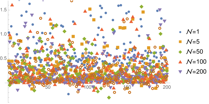
(a) 200 random realizations of the ASIP

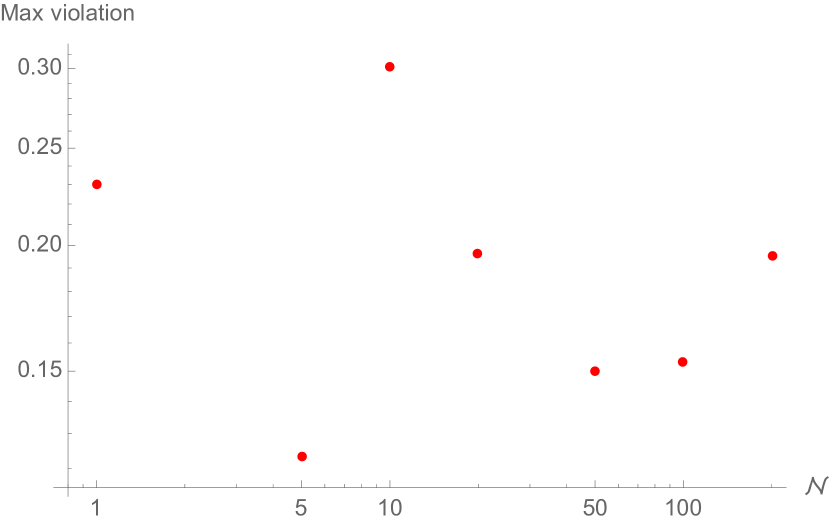
(b) The negative of minimal value of $\frac{\mathcal{F}-\mu^{\prime\prime}(0)}{\mu^{\prime\prime}(0)}$ out of all the random realizations for each $\mathcal{N}$ – the max violation.

Figure 3: The value of $\frac{\mathcal{F}-\mu^{\prime\prime}(0)}{\mu^{\prime\prime}(0)}$ in the random ASIP of $N=2$ particles and $L=3$ sites with periodic boundary conditions. We present $200$ random realizations for each $\mathcal{N}$ value, where the rates $p_{\pm}(x)\in\left[0,1\right]$ are randomized. (a) While most realizations at any $\mathcal{N}$ satisfy the bound, there are violations. The maximal violations of each $\mathcal{N}$ are plotted in (b). They does not vanish with increasing $\mathcal{N}$.

Appendix E Derivation of the series activity bound: the kinetic uncertainty relation

In this section, we use (13) derive a bound on the current variance in terms of the series activity $\langle A^{\perp}\rangle$ also known in the literature as the kinetic uncertainty relation Di Terlizzi and Baiesi (2019); Shiraishi (2020); Pal et al. (2021a). Let us start from (13) and take $Y_{x,y}=\alpha\langle j_{x,y}\rangle$ for some constant $\alpha$. Notice that this choice immediately satisfies the Kirchhoff’s junction rule (10). From (13), we then find the following inequality

$$\frac{1}{2}\mu^{\prime\prime}(0) \geq\alpha\mu^{\prime}_{j}-\alpha^{2}\sum_{x,y>x}\frac{\langle j_{y,x}\rangle^{2}}{\langle a_{x,y}\rangle}$$ (30)

$$=\alpha\mu^{\prime}_{j}-\alpha^{2}\sum_{x,y>x}\langle a_{x,y}\rangle\frac{\langle j_{y,x}\rangle^{2}}{\langle a_{x,y}\rangle^{2}}.$$

Notice that since $|\langle j_{y,x}\rangle/\langle a_{x,y}\rangle|\leq 1$, we obtain

$$\frac{1}{2}\mu^{\prime\prime}(0)\geq\alpha\mu^{\prime}_{j}-\frac{1}{2}\alpha^{2}\langle A^{\perp}\rangle.$$ (31)

Now, it is straight-forward to choose $\alpha=\mu^{\prime}_{j}/\langle A^{\perp}\rangle$ to obtain the kinetic uncertainty bound

$$\mu^{\prime\prime}(0)\geq\frac{(\mu^{\prime}_{j})^{2}}{\langle A^{\perp}\rangle},$$ (32)

that was obtained in Di Terlizzi and Baiesi (2019); Shiraishi (2020); Pal et al. (2021a).

References

- Barato and Seifert (2015) A. C. Barato and U. Seifert, Phys. Rev. Lett. 114, 158101 (2015).
- Gingrich et al. (2016) T. R. Gingrich, J. M. Horowitz, N. Perunov, and J. L. England, Phys. Rev. Lett. 116, 120601 (2016).
- Horowitz and Gingrich (2020) J. M. Horowitz and T. R. Gingrich, Nature Physics 16, 15 (2020).
- Pal et al. (2021a) A. Pal, S. Reuveni, and S. Rahav, Phys. Rev. Research 3, 013273 (2021a).
- Macieszczak et al. (2018) K. Macieszczak, K. Brandner, and J. P. Garrahan, Phys. Rev. Lett. 121, 130601 (2018).
- Shiraishi (2020) N. Shiraishi, arXiv:2106.11634 (2020).
- Pal et al. (2021b) A. Pal, S. Reuveni, and S. Rahav, Phys. Rev. Research 3, L032034 (2021b).
- Fischer et al. (2018) L. P. Fischer, P. Pietzonka, and U. Seifert, Phys. Rev. E 97, 022143 (2018).
- Gingrich and Horowitz (2017) T. R. Gingrich and J. M. Horowitz, Phys. Rev. Lett. 119, 170601 (2017).
- Hasegawa (2021) Y. Hasegawa, Phys. Rev. Lett. 126, 010602 (2021).
- Miller et al. (2021) H. J. D. Miller, M. H. Mohammady, M. Perarnau-Llobet, and G. Guarnieri, Phys. Rev. Lett. 126, 210603 (2021).
- Hasegawa (2020) Y. Hasegawa, Phys. Rev. Lett. 125, 050601 (2020).
- Liu and Segal (2019) J. Liu and D. Segal, Physical review. E 99 6-1, 062141 (2019).
- Horowitz and Gingrich (2017) J. M. Horowitz and T. R. Gingrich, Phys. Rev. E 96, 020103 (2017).
- Soret et al. (2020) A. Soret, O. Shpielberg, and E. Akkermans, arXiv:2011.07246 (2020).
- Shiraishi et al. (2018) N. Shiraishi, K. Funo, and K. Saito, Phys. Rev. Lett. 121, 070601 (2018).
- Falasco et al. (2020) G. Falasco, M. Esposito, and J.-C. Delvenne, New Journal of Physics 22, 053046 (2020).
- Polettini et al. (2021) M. Polettini, G. Falasco, and M. Esposito, arXiv:2106.00425 (2021).
- Shpielberg and Nemoto (2019) O. Shpielberg and T. Nemoto, Phys. Rev. E 100, 032104 (2019).
- Manikandan and Krishnamurthy (2018) S. K. Manikandan and S. Krishnamurthy, Journal of Physics A: Mathematical and Theoretical 51, 11LT01 (2018).
- Derrida et al. (2004) B. Derrida, B. Doucot, and P.-E. Roche, J. Stat. Phys. 115, 717 (2004).
- Bertini et al. (2015) L. Bertini, A. De Sole, D. Gabrielli, G. Jona-Lasinio, and C. Landim, Rev. Mod. Phys. 87, 593 (2015).
- Maes and Netočný (2008) C. Maes and K. Netočný, EPL (Europhysics Letters) 82, 30003 (2008).
- Monthus (2019) C. Monthus, J. Phys. A: Math. Theor. 52, 135003 (2019).
- Spohn (2014) H. Spohn, J. Stat. Phys. 154, 1191–1227 (2014).
- Meerson and Smith (2019) B. Meerson and N. R. Smith, J. Phys. A: Math. Theor. 52, 415001 (2019).
- Gabrielli and Renger (2020) D. Gabrielli and D. R. M. Renger, J. Stat. Phys. 181, 2353–2371 (2020).
- Baek et al. (2016) Y. Baek, Y. Kafri, and V. Lecomte, J. Stat. Mech. 2016, 053203 (2016).
- Reuveni et al. (2012) S. Reuveni, I. Eliazar, and U. Yechiali, Phys. Rev. Lett. 109, 020603 (2012).
- Grosskinsky et al. (2011) S. Grosskinsky, F. Redig, and K. Vafayi, J. Stat. Phys. 142, 952 (2011).
- Iwase et al. (2013) T. Iwase, A. Tajima, S. Sugimoto, K.-i. Okuda, I. Hironaka, Y. Kamata, K. Takada, and Y. Mizunoe, Sci. Rep. 3, 3081 (2013).
- Svetlizky and Roichman (2021) I. Svetlizky and Y. Roichman, Physical Review Letters 127, 038003 (2021).
- Seifert (2012) U. Seifert, Reports on progress in physics 75, 126001 (2012).
- Van den Broeck and Esposito (2015) C. Van den Broeck and M. Esposito, Physica A: Statistical Mechanics and its Applications 418, 6 (2015).
- Barato et al. (2018) A. C. Barato, R. Chetrite, A. Faggionato, and D. Gabrielli, New J. Phys. 20, 103023 (2018).
- Sedrakyan and Sedrakyan (2018) H. Sedrakyan and N. Sedrakyan, Algebraic inequalities (Springer, 2018).
- Di Terlizzi and Baiesi (2019) I. Di Terlizzi and M. Baiesi, J. Phys. A 52, 02LT03 (2019).
- Note (1) As usual, we discard here logarithmic corrections, normalization and corrections to the action.
- Dechant and Sasa (2018) A. Dechant and S.-i. Sasa, J. Stat. Mech. 2018, 063209 (2018).
- Note (2) There is some freedom in this definition as we wish to control only the steady densities and currents.
- Dechant and Sasa (2020) A. Dechant and S.-i. Sasa, arXiv:2010.14769 (2020).
- Note (3) In fact, short range jumps is a sufficient conditions, but more tedious to treat and harder to precisely define on a short 1D chain.
- Shpielberg et al. (2017) O. Shpielberg, Y. Don, and E. Akkermans, Phys. Rev. E 95, 032137 (2017).
- Shpielberg (2017) O. Shpielberg, Phys. Rev. E 96, 062108 (2017).
- Nemoto et al. (2017) T. Nemoto, R. L. Jack, and V. Lecomte, Phys. Rev. Lett. 118, 115702 (2017).
- Shpielberg et al. (2018) O. Shpielberg, T. Nemoto, and J. a. Caetano, Phys. Rev. E 98, 052116 (2018).
- Gerschenfeld and Derrida (2011) A. Gerschenfeld and B. Derrida, EPL (Europhysics Letters) 96, 20001 (2011).
- Nguyen et al. (2021) M. Nguyen, Y. Qiu, and S. Vaikuntanathan, Annual Review of Condensed Matter Physics 12, 273 (2021).
- Howard and Hyman (2003) J. Howard and A. A. Hyman, Nature 422, 753 (2003).
- Howard and Hyman (2009) J. Howard and A. A. Hyman, Nature Reviews Molecular Cell Biology 10, 569 (2009).