Shadows of Lorentzian traversable wormholes

Abstract

The prospect of identifying wormholes by investigating the shadows of wormholes constitute a foremost source of insight into the evolution of compact objects and it is one of the essential problems in contemporary astrophysics. The nature of the compact objects (wormholes) plays a crucial role on shadow effect, which actually arises during the strong gravitational lensing. Current Event Horizon Telescope observations have inspired scientists to study and to construct the shadow images of the wormholes. In this work, we explore the shadow cast by a certain class of rotating wormhole. To search this, we first compose the null geodesics and study the effects of the parameters on the photon orbit. We have exposed the form and size of the wormhole shadow and have found that it is slanted as well as can be altered depending on the different parameters present in the wormhole spacetime. We also constrain the size and the spin of the wormhole using the results from M87* observation, by investigating the average diameter of the wormhole as well as deviation from circularity with respect to the wormhole throat size. In a future observation, this type of study may help to indicate the presence of a wormhole in a galactic region.

Keywords : Wormhole; Shadow ; Null geodesics

I Introduction:

Invisible astrophysical objects, like wormholes are still a matter of disquiet since the discovery of geometrical theory of gravity. Wormholes are topologically non-trivial structures of the spacetime connecting our Universe with other universes. The original idea was known as the Einstein-Rosen bridge Einstein , and was more of a mathematical concept, since it did not deal with traversable wormholes. Later Moris and Thorne kg14 developed the idea of traversable wormholes containing exotic matter in their throat. More developments were carried out by various other researchers Gon ; Ellis ; kg1 . In observational astrophysics, wormholes are still a viable subject. Observational detection means one has to interact with the geometrical structure of the wormhole by which data is acquired. Therefore, scientists are trying to envisage wormholes in order to acquire perception about its geometrical features. Apart from gravitational lensing effects GL1 , another possible method for probing wormholes is the usage of shadows (a dark region over a luminous contextual). One can recognize the shadow of a wormhole as the result of strong gravitational lensing generating a dark spot in the sky of a remote viewer. It is actually an optical look exhibited by the wormhole when there is a source of light from stars, accretion flows etc. around it. This manifestation has been investigated theoretically as well as observationally, by the application of very large baseline interferometry (VLBI) Doe techniques at sub-mm wavelengths, for studying the shadow cast by supermassive objects, including the ongoing ambitious project involving Sagittarius A* in our galaxy center Brod2 . Being at sub mm wavelength this technique significantly reduces the interstellar scattering, and may allow us to see beyond the compact synchrotron emitting region around SgrA*, since this region is expected to become optically thin at sub-mm wavelengths. Also, VLBI experiments can reach a resolution of the order of the angular size of the gravitational radius of SgrA*. Thus the spacetime geometry could be determined through the analysis of shadow in the vicinity of photon sphere. Similar ambitious projects include the Japanese VLBI Network (JVN), the Chinese VLBI Network (CVN), the Korean VLBI Network (KVN), the Chinese Space VLBI project VLBI .

Compact Objects can cause extreme local deflections of light and can bend light by an arbitrary large angle, causing the formation of light rings which are circular photon spheres, possessing distinct phenomenological signatures in terms of both electromagnetic and gravitational waves. And since this shadow outline depends on the gravitational lensing of nearby radiation, its proper surveillance can provide evidence about the parameters as well as spacetime geometry around the wormhole. Light propagation i.e. null geodesics in compact object (wormhole) spacetime can be perceived in two ways: trajectories which escape to distant observer and such that are apprehended by the compact object. Therefore, a black region appears in the viewer’s sky, creating the shadow. The boundary of the shadow can be resolved by the wormhole spacetime metric itself, as it relates to the appearing shape of the photon detained orbits as observed by a remote viewer. Theoretically, although we seek to find an analytical closed form of the shadow edge, it is rarely possible to integrate the geodesic motion. In such cases the null geodesic equations have to be solved numerically. An efficient procedure involves a method called backwards ray-tracing, which requires the propagation of light rays from the observer backward in time and identifying their origin Backtracing , instead of evolving the light rays directly from a light source and detect the ones that reach the observer.

Ever since the remarkable image of the shadow of black holes, M87* at the center of the Virgo A galaxy was taken by Event Horizon Telescope in April 2019 telescope ; telescope2 , a new era of research on shadows of dark compact objects like black holes and wormholes have emerged. Following this, in 2020, Kruglov BS6 considered rational nonlinear electrodynamics and interpreted the super-massive M87* black hole as a regular (without singularities) magnetized black hole. The shadow observed from the center of M87* was consistent with the shadow generated through numerical simulation of a Kerr black hole of mass $(6.5\pm 0.7)^{9}M_{\odot}$ telescope . This shadow can provide us with the properties of the black hole such as mass, spin, accretion disk and to verify the constraints on fundamental physics. The EHT data strongly suggest that the dimensionless spin parameter $a*$ is $\gtrsim 0.5$. This results in the non-existence of ultra-light boson of mass $\mu_{b}\sim 10^{-21}$eV, which was considered as a dark matter candidate in the distribution scales of $\sim$ kpc dav . Vagnozzi and Visinelli vagn used the M87* data to constraint the AdS₅ curvature radius in Randall-Sundrum AdS₅ brane-world.

Since in classical theory these black holes are not a source of radiation, the shadow actually targets exactly this feature, for lack of radiation. The shadow is an important observational evidence of the most standard problem in general relativity: the motion of light around compact objects. Earliest works on static Schwarzschild black hole shadows are done by Syn and Luminet . The influence of charge on the measurements of shadow in case of Riessner-Nordström black hole were investigated by Zakharov et.al. Zakharov1 ; Zakharov2 . Detailed study on rotating Kerr black hole were conducted by Bardeen -Brod to mention a few. Other pioneering works on black hole shadows include Yumoto -sha12 . The challenge of investigating the spacetime in the vicinity of the event horizon of a black hole, with angular resolution comparable to the event horizon, is almost a thing of the past. In fact direct detection of dynamics of matter at light speed and at strong gravity near a compact object is now almost possible. Very recently in 2020, shadow, quasinormal modes, and quasiperiodic oscillations of rotating Kaluza-Klein black holes were investigated by Ghasemi-Nodehi et.al. BS1 , while Kala et al. BS2 studied the deflection of light and shadow cast by a dual-charged stringy black hole. Long et al. BS3 shown that the shadow size of disformal Kerr black hole in non-stealth rotating solutions in quadratic degenerate higher-order-scalar-tensor (DHOST) increases with a deformation parameter and the shape on both deformation and spin parameter. Quasi-normal modes and shadows of Schwarzschild and high-dimensional Einstein-Yang-Mills spacetimes were also discussed in BS5 -BS11 .

While black holes continues to attract much attention, horizonless compact objects are fast gaining popularity recently in the literature for a number of reasons (for a review of the topic, see the recent work of Cardoso and Pani cardoso ). One important class of horizonless objects are wormholes. Imaging the shadow of a wormhole may help to progress observational investigation of differentiating the wormhole amongst other compact objects e.g. black holes, neutron stars etc. In an interesting paper in 2013, Bambi Bambi_2013 pointed out that there is insufficient evidence to confirm that the supermassive objects at the center of many galaxies, including our own, are in fact Kerr black holes. Instead exotic compact objects like wormholes might have been formed in the early universe. Though an exhaustive list of papers on wormhole shadows is not possible, yet Sarbach -Vincent are many notable works. More recently, Amir et. al. WS1 worked on the shadows of Kerr like wormholes and charged wormholes WS2 in Einstein-Maxwell-dilaton theory. Shadows of rotating wormholes were also investigated by Gyulchev et.al. WS3 , Shaikh WS4 and Abdujabbarov WS5 . Wielgus et al. BS4 constructed Reissner-Nordstr$\ddot{o}$m (RN) wormhole by joining two different RN spacetime i.e. two different mass and charge. This kind of wormholes are not mirror-symmetric which affects the photon sphere and may have two photon rings to a distant observer. This doubling of photon ring was explained by doubling of effective potential maximum. However, mirror-symmetric wormholes can also have multiple photon rings and can exhibit interesting strong lensing effect (RS2019 ; RS2019b ; NT2021 ). These recent ventures WS6 on the shadow of compact objects have inspired us to construct the shadow of wormholes, as well as, analyse the shape of the shadows.

The paper is organized as follows: in section II we have described the motion of photons around wormholes. The geometric equations defining its shadow are obtained in section III. Section VI is dedicated to final observations.

Figure 1: Schematic diagram of ergosphere. The region between the ergosurface (red-dashed curve) and the wormhole throat (blue circle) is the ergoregion.

II The general rotating wormhole spacetime

Let us consider a general stationary, axisymmetric spacetime metric, describing a Teo class rotating traversable wormhole Teo in Boyer-Linquist coordinates $(t,r,\theta,\phi)$ as

$$ds^{2} = -N^{2}dt^{2}+\left(1-\frac{b}{r}\right)^{-1}dr^{2}+r^{2}K^{2}\left[d\theta^{2}+\sin^{2}\theta(d\phi-\omega~{}dt)^{2}\right],$$ (1)

where the spherical polar coordinates $t,r,\theta$ and $\phi$ are defined by $-\infty<t<\infty$, and $r_{0}\leq r<\infty,~{}0\leq\theta\leq\pi$ and $0\leq\phi\leq 2\pi$ and in general, the metric functions $N,b,K$ and $\omega$ depend only on $r$ and $\theta$. The orbits of the timelike and the spacelike Killing fields ($t^{\mu}\partial_{\mu}=\partial_{t}$ and $\phi^{\mu}\partial_{\mu}=\partial_{\phi}$ respectively ) represent in terms of the parameters $t$ and $\phi$. This metric is actually a generalized rotating form of the static Morris-Thorne wormhole metric kg14 . Therefore, the metric functions must have some restrictions, which lead to the specific geometry and significant properties of the wormhole. The function $N$ which regulates the gravitational redshift is often called a redshift function. In order for the wormhole to be traversable, one has to ensure that there are no curvature singularities or event horizons. Therefore, the redshift function $N$ should be nonzero and finite all over the region, i.e. from the throat to the spatial infinity. The function $b$ is known as the shape function which regulates the shape of the wormhole. It is always non-negative and possesses an apparent singularity at $r=r_{0}=b\geq 0$, which is associated with the throat of the wormhole. The function $b$ should be independent of $\theta$ to avoid any curvature singularity at the throat i.e. it obeys the restriction $\frac{\partial b(r,\theta)}{\partial\theta}=0$. An important constraint is the flare-out condition at the throat: $\partial_{r}b|_{r=r_{0}}<1$, while $b(r)<r$ near the throat. Function $K(r,\theta)$ is a regular, positive and non-decreasing function, defining the proper radial distance $R=rK$, measured at $(r,\theta$) from the origin. Actually it regulates the area radius given by $R$. The function $\omega$ is associated with the angular velocity of the wormhole. Also to confirm that metric (1) is regular on the rotation axis $\theta=0,~{}\pi$, the derivatives of $N$ and $K$ with respect to $\theta$ should vanish on it, i.e. $\frac{\partial N(r,\theta)}{\partial\theta}=0$, $\frac{\partial K(r,\theta)}{\partial\theta}=0$. Although, a wide variety of choices for the metric functions $N,K,b$ and $\omega$ can be freely adopted, we emphasize that all the solutions do not correspond to wormhole physics. One must choose such metric functions which satisfy the above-mentioned regularity conditions. That class of solutions are the certain cases of the rotating Teo wormhole. In this study we will consider the specific type of solutions, where entire metric coefficients are functions of radial coordinate r only. These solutions reduce to the static wormhole for zero rotation, i.e. when $\omega=0$.

Recently, Konoplya and Zhidenko (RK2016, ) studied quasinormal rings of a wormhole, which rings like the Schwarzschild or the Kerr black holes and its metric is similar to (1). The specific form of $g_{tt}$ and the shape function $b(r)$ are given by

$$N = \sqrt{1-{2M\over r}}~{}~{},~{}~{}~{}b(r)={r_{0}^{2}+2M(r-r_{0})\over r},~{}~{}\omega={2J\over r^{3}}={2aM^{2}\over r^{3}}~{}~{},~{}~{}~{}K=1.$$ (2)

Here $a=J/M^{2}$ is the spin parameter. This wormhole has mass $M$ and a throat at $r_{0}\geq 2M\geq 0$.

An ergoregion may be present around the throat of a rotating wormhole. This region can be determine when $g_{tt}=-(N^{2}-\omega^{2}r^{2}\sin^{2}\theta)\geq 0$ and the ergosurface by $g_{tt}=0$. The ergosurface for the metric (1) is given by

$$N^{2}-\omega^{2}r^{2}K^{2}\sin^{2}\theta=0.$$ (3)

Since the ergoregion doesn’t extent up to the poles $\theta=0$ and $\theta=\pi$, there exist a critical angle $\theta_{c}$, where the ergosphere exists in between $\theta_{c}$ and $\pi-\theta_{c}$, for all $0<\theta_{c}\leq\pi/2$. This critical angle can determined at the throat of the wormhole using eq. (3) as

$$\sin\theta_{c}=\left|{N_{0}\over\omega_{0}r_{0}K_{0}}\right|$$ (4)

Further, the ergosphere will only exist when the spin parameter $a$ crosses a critical limit $a_{c}$, corresponding to $\sin\theta_{c}=1$ or $\omega_{c}=N_{0}/r_{0}K_{0}$. For the wormhole metric (2) with $M=1$ and $r_{0}=2.2$, the critical value is $a_{c}=0.729657$. The ergosphere for these values can be seen in Fig. 1.

III Propagation of light in a rotating wormhole spacetime

When a wormhole is between a star (bright source of light) and a viewer, the light comes to the viewer after being deviated by the gravitational field of wormhole. However, certain portion of the photons (with small impact parameters) emanated by the star end up falling into the wormhole, i.e. not able to reach the observer, giving as a result, a dark sector in the sky dubbed as shadow. The boundary of the shadow apparently is determined by unstable circular photon orbits. In order to find the unstable orbit, one is required to study the geodesic configuration.

The motion of a photon in the rotating wormhole spacetime (1) can be described by the Lagrangian, (${\textbf{\L}}=\frac{1}{2}g_{\mu\nu}\dot{x}^{\mu}\dot{x}^{\nu}$) as:

$${\textbf{2\L}}=-N^{2}\dot{t}^{2}+\frac{\dot{r}^{2}}{1-b/r}+r^{2}K^{2}[~{}{\dot{\theta}}^{2}+\sin^{2}\theta(\dot{\phi}-\omega\dot{t})^{2}~{}].$$ (5)

Here an overdot denotes the derivative with respect to the affine parameter $\lambda$. Here the Lagrangian does not depend on $t$ and $\phi$, as a result, we have only two constants of motion, which are the energy $E$ and the angular momentum $L$ in the direction of the axis of symmetry of the photon.

$$p_{t} = \frac{\partial{\textbf{\L}}}{\partial\dot{t}}=-N^{2}\dot{t}-\omega r^{2}K^{2}\sin^{2}\theta(\dot{\phi}-\omega\dot{t})=-E,$$

$$p_{\phi} = \frac{\partial{\textbf{\L}}}{\partial\dot{\phi}}=r^{2}K^{2}\sin^{2}\theta(\dot{\phi}-\omega\dot{t})=L.$$

These two equations yield:

$$\dot{t}=\frac{E-\omega L}{N^{2}},~{}~{}~{}\dot{\phi}=\frac{L}{r^{2}K^{2}\sin^{2}\theta}+\frac{\omega(E-\omega L)}{N^{2}}.$$ (6)

Now, we calculate the $r$ and $\theta$-component of the momentum as,

$$p_{r}=\frac{\partial\textbf{\L}}{\partial\dot{r}}=\frac{\dot{r}}{1-\frac{b}{r}},~{}~{}~{}p_{\theta}=\frac{\partial\textbf{\L}}{\partial\dot{\theta}}=r^{2}K^{2}\dot{\theta}.$$ (7)

To achieve a general formula for finding the contour of a shadow we use Hamilton-Jacobi method for the null geodesic equations in the general rotating spacetime (1). The Hamilton-Jacobi method determines the geodesics via the equation

$$\frac{\partial S}{\partial\lambda}=-\frac{1}{2}g^{\mu\nu}\frac{\partial S}{\partial x^{\mu}}\frac{\partial S}{\partial x^{\nu}},$$ (8)

where $\lambda$ is the affine parameter along the geodesics, $g_{\mu\nu}$ are the components of the metric tensor, and $S$ is the Jacobi action with the following separable ansatz,

$$S=\frac{1}{2}\mu^{2}\lambda-Et+L\phi+S_{r}(r)+S_{\theta}(\theta),$$ (9)

where $S_{r}$ and $S_{\theta}$ are the functions of $r$ and $\theta$, respectively and $\mu$ is the mass of the test particle. For photons, $\mu=0$. Here the rotating wormhole metric functions $N,~{}b,~{}K$ and $\omega$, depend only on the radial coordinate, therefore, following Ned , the Hamilton-Jacobi equation will be separable. Inserting Eq. (9) into Eq. (8) one can obtain the following equations for the functions $S_{r}(r)$ and $S_{\theta}(\theta)$ Ned :

$$\left(\frac{dS_{\theta}}{d\theta}\right)^{2}=Q-\frac{L^{2}}{\sin^{2}\theta},$$ (10)

$$\left(1-\frac{b}{r}\right)N^{2}\left(\frac{dS_{r}}{dr}\right)^{2}=(E-\omega L)^{2}-\Big{(}\mu^{2}N^{2}+Q\frac{N^{2}}{r^{2}K^{2}}\Big{)},$$ (11)

where $Q$ is the Carter constant.

We know $p_{r}=\frac{\partial S}{\partial r}=\frac{dS_{r}}{dr}$ and $p_{\theta}=\frac{\partial S}{\partial\theta}=\frac{dS_{\theta}}{d\theta}$, therefore, equations (7), (10) and (11) yield Ned ,

$$\frac{N}{\sqrt{1-b/r}}\frac{dr}{d\lambda}=\pm\sqrt{R(r)},~{}~{}~{}r^{2}K^{2}\frac{d\theta}{d\lambda}=\pm\sqrt{T(\theta)},$$ (12)

where,

$$T(\theta) = Q-\frac{L^{2}}{\sin^{2}\theta},$$ (13)

$$R(r) = (E-\omega L)^{2}-\left(\mu^{2}N^{2}+Q\frac{N^{2}}{r^{2}K^{2}}\right).$$ (14)

Hence, the Jacobi action assumes the following form,

$$S=\frac{1}{2}\mu^{2}\lambda-Et+L\phi+\int\sqrt{\frac{R(r)}{N^{2}(1-b/r)}}~{}dr+\int\sqrt{T(\theta)}~{}d\theta.$$ (15)

The geodesic equations in stationary and axisymmetric spacetimes are parameterized by the constants of motions $E,~{}L$ and $Q$. However, the geodesic motion of a photon is described by two independent parameters defined by:

$$\xi=\frac{L}{E},~{}~{}~{}\eta=\frac{Q}{E^{2}}.$$

Here, $\xi$ and $\eta$ are known as impact parameters and a new affine parameter $\widetilde{\lambda}=\lambda E$. After eliminating the energy from the geodesic equations, the path of the photon is parameterized only by $\xi$ and $\eta$. One can write the functions $R(r)$ and $T(\theta)$ in terms of the impact parameters as,

$$R(r) = (1-\omega\xi)^{2}-\eta\frac{N^{2}}{r^{2}K^{2}},$$ (16)

$$T(\theta) = \eta-\frac{\xi^{2}}{\sin^{2}\theta}.$$ (17)

For a photon $\mu=0$.

IV Wormhole shadow

Figure 2: Schematic diagram of the photon orbits around the wormholes.

Two regions of spacetime are joined through wormhole (a tunnel-like structure, without any horizon or singularity within it). Let us assume that the photons are coming from a star towards the wormhole, (placed between the observer and the star) and illuminate one region, and no light sources are remaining in the neighborhood of the throat in the other region. In the first region, the possible orbit of the photons around the wormhole are as follows: (i) orbits entering into the wormhole and passing through its throat (ii) dispersed from the wormhole to infinity. A remote viewer will be capable of observing only dispersed photons from the wormhole (see figure 2). However the photon apprehended by the wormhole will form a dark patch. This dark region detected on the bright background is known as shadow of the wormhole. To find the wormhole shadow, i.e. dark region in the viewer’s atmosphere in the presence of a shiny background, one would have to start finding out the critical orbits that separate the evading and falling photons. Actually our prime motive is to estimate these critical geodesics or unstable circular orbits. In order to acquire the boundary of the wormhole shadow, one needs to study the radial motion of photons around the wormholes. The critical orbits (described by certain critical values of the impact parameters $\xi$ and $\eta$ ) distinguish the dispersed and apprehended photons. A slight disturbance in these critical values can change it either to a seepage or to a apprehend orbit. As a result, the critical impact parameters describe the boundary of a shadow. Thus the boundary of the shadow is determined by the unstable circular photon orbits. By studying the radial geodesic equation, one can calculate the critical orbit, which can be expressed in the form of an energy conservation equation,

$$\left(\frac{dr}{d\bar{\lambda}}\right)^{2}+V_{eff}=1,~{}~{}V_{eff}=1-\frac{1}{N^{2}}\left(1-\frac{b}{r}\right)R(r),$$ (18)

where $V_{eff}$ is the effective potential that describes the geodesic motion of a photon around the wormhole. The null geodesics are divided into two classes depending on their impact parameters: (i) trajectories of photon passing through the wormhole (ii) orbits of the photon dispersing to infinity. The boundary among the two classes is destined through a family of unstable spherical orbits fulfilling the following conditions,

$$V_{eff}=1,~{}~{}~{}\frac{V_{eff}}{dr}=0,~{}~{}~{}\frac{d^{2}V_{eff}}{dr^{2}}\leq 0.$$ (19)

Figure 3: Shadow of a wormhole for different $a$ and $r_{0}=2.5$. The axes are in units of $M$.

Figure 4: Shadow of a wormhole for different $r_{0}$ and $a=0.8$. The axes are in units of $M$.

The first condition comes from the fact that the radial motion has a turning point $dr/d\bar{\lambda}=0$, when the photon will scatter from the wormhole. The last conditions are due to the maximum of the effective potential for the critical orbit between seepage and plunge motion.

While writing down the above conditions in terms of $R(r)$, one could assume that the functions $N$ and $(1-\frac{b}{r})$ are finite and non-zero outside the throat of the wormhole. Therefore, for the unstable circular orbits lying outside the throat, i.e., having radii greater than $r_{0}$, the above set of conditions can be written in terms of $R(r)$ as,

$$R(r)=0,~{}~{}~{}\frac{dR}{dr}=0,~{}~{}~{}\frac{d^{2}R}{dr^{2}}\geq 0.$$ (20)

Using the equations $R(r)=0,~{}~{}dR/dr=0$, one can easily find two expressions for the impact parameters $\xi$ and $\eta$ in terms of the radial coordinate of the unstable circular orbit as,

$$\eta = \frac{r^{2}K^{2}}{N^{2}}(1-\omega\xi)^{2},$$ (21)

$$\xi = \frac{\Sigma}{\Sigma\omega-\omega^{{}^{\prime}}},~{}~{}~{}\Sigma=\frac{1}{2}\frac{d}{dr}\ln\left(\frac{N^{2}}{r^{2}K^{2}}\right).$$ (22)

Here prime denotes the differentiation with respect to radial coordinate $r$. This process of finding the location of the unstable spherical orbits in the impact parameter space as given in equations (21) and (22) was originally derived in Ned . However, it has been shown that a wormhole throat can act as a natural location of unstable circular orbits (RS2019, ). For such unstable orbits, $(1-b/r)$ vanishes and hence, $V_{eff}=1$ is automatically satisfied. Therefore, for unstable circular orbits located at the throat, the second conditions in (19) can be reduced to (WS4, ),

$$(1-\omega_{0}\xi)^{2}-\eta\frac{N_{0}^{2}}{r_{0}^{2}K_{0}^{2}}=0,$$ (23)

where the subscript ‘0’ implies that the functions are evaluated at the throat.

Figure 5: Shadow of a wormhole (red solid curve) and a Kerr black hole (blue dashed curve) for different $a$. Here $r_{0}=3.0$. The axes are in units of $M$.

For the set of unstable photon orbits, equations (21), (22) and (23) express the critical locus of the impact parameters. In other words, these equations express the boundary of the shadow in the impact parameter space. However, for true observation, the remote viewer will see the apparent shape of a shadow in his sky (a plane passing through the center of the wormhole and normal to the line linking it with the viewer). The celestial coordinates connected to the actual astronomical measurements that span a two-dimensional plane are defined as vaz ,

$$\alpha = \lim_{r_{o}\rightarrow\infty}\left(-r_{o}^{2}\sin\theta_{o}\left[\frac{d\phi}{dr}\right]_{(r_{o},\theta_{o})}\right),$$ (24)

$$\beta = \lim_{r_{o}\rightarrow\infty}\left(r_{o}^{2}\left[\frac{d\theta}{dr}\right]_{(r_{o},\theta_{o})}\right),$$ (25)

where $r_{o}$ is the position coordinate of the remote viewer taken very large (far away from the wormhole) and $\theta_{o}$ is the angular coordinate. It is actually the angle of inclination between the axis of symmetry of the wormhole and the direction to the viewer.

Figure 6: Shadow of a wormhole (red solid curve) and a Kerr black hole (blue dashed curve) for different $r_{0}$. Here $a=0.8$. The axes are in units of $M$.

The celestial coordinates $\alpha$ and $\beta$ are the discernible perpendicular distances of the shadow image, as observed from the rotation axis and from its projection on the equatorial plane respectively. Using the geodesic equations and values of the four-velocity components and after some simple algebraic manipulation, the celestial coordinates assume the following forms:

$$\alpha = -\frac{\xi}{\sin\theta_{0}},$$ (26)

$$\beta = \left(\eta-\frac{\xi^{2}}{\sin^{2}\theta_{0}}\right)^{1/2}.$$ (27)

After knowing the expressions of celestial coordinates and impact parameters, one can construct the shadow of wormholes. In the $(\alpha,\beta)$-plane, Eqs. (21), (22), (26) and (27) define the part of the shadow boundary formed by the unstable circular orbits which lie outside the throat. However, the part of the shadow boundary formed due to the unstable circular orbits which are located at the throats, we obtain, from Eqs. (23), (26) and (27),

$$(N_{0}^{2}-\omega_{0}^{2}r_{0}^{2}K_{0}^{2}\sin^{2}\theta_{obs})\alpha^{2}-2\omega_{0}r_{0}^{2}K_{0}^{2}\sin\theta_{obs}\,\alpha-r_{0}^{2}K_{0}^{2}+N_{0}^{2}\beta^{2}=0.$$ (28)

Therefore, the complete contour of the shadow is given by the combination of Eq. (26)-(27) [with $\xi$ and $\eta$ given by Eq. (21) and (22)] and Eq. (28) (WS4, ).

Figures 3 and 4 show the shadow the wormhole given above for different values of the spin and throat size. Note that, for a given wormhole size $r_{0}$, the shadow shape deviates from circularity as we increase the spin $a$ (see fig. 3). On the other hand, for a given spin $a$, the shadow becomes more and more circular as we increase the wormhole size $r_{0}$ (see fig. 4). We also have compared our results with those of a Kerr black hole in figs. 5 and 6. Note that, for small spin and smaller wormhole size, its shadow mimics those of the black hole. However, with increasing either the spin or the throat size, the shadow of a wormhole start deviating from that of a Kerr black hole. Detection of such deviation may possibly indicate the presence of a wormhole.

V Constraining the wormhole parameters using the M87^∗ results

We now constrain the size and the spin of the wormhole using the results from M87^∗ observation telescope . For this purpose, we use the average angular size of the shadow and its deformation from circularity. Since the shadow has reflection symmetry with respect to the $\alpha$-axis, its geometric center $(\alpha_{c},\beta_{c})$ is given by $\alpha_{c}=1/A\int\alpha dA$ and $\beta_{c}=0$, $dA$ being an area element. We first define an angle $\phi$ between the $\alpha$-axis and the vector connecting the geometric centre $(\alpha_{c},\beta_{c})$ with a point $(\alpha,\beta)$ on the boundary of a shadow. Therefore, the average radius $R_{av}$ of the shadow is given by. Bambi

$$R_{av}^{2}=\frac{1}{2\pi}\int_{0}^{2\pi}l^{2}(\phi)\;d\phi,$$ (29)

where $l(\phi)=\sqrt{[\alpha(\phi)-\alpha_{c}]^{2}+\beta(\phi)^{2}}$ and $\phi=\tan^{-1}[\beta(\phi)/(\alpha(\phi)-\alpha_{c})]$. Following telescope , we define the deviation $\Delta C$ from circularity as,

$$\Delta C=\frac{1}{R_{av}}\sqrt{\frac{1}{2\pi}\int_{0}^{2\pi}(l(\phi)-R_{av})^{2}\;d\phi}.$$ (30)

Note that $\Delta C$ is the fractional RMS distance from the average radius of the shadow.

According to EHT collaboration telescope , the angular size of the observed shadow is $\Delta\theta_{sh}=42\pm 3$ $\mu$as, and the deviation $\Delta C$ is less than $10\%$. Also, following telescope , we take the distance to M87^∗ to be $D=(16.8\pm 0.8)$ Mpc and the mass of the object to be $M=(6.5\pm 0.7)\times 10^{9}M_{\odot}$. These numbers imply that the average diameter of the shadow should be,

$$\frac{d_{sh}}{M}=\frac{D\Delta\theta_{sh}}{GM}=11.0\pm 1.5,$$ (31)

where the errors have been added in quadrature. The above quantity must be equal to $\frac{2R_{av}}{M}$. In Fig. 7, we have shown the average diameter and the deviation from circularity of the shadow for different values of the spin and the wormhole throat size. Here, we have taken the inclination angle to be $\theta_{o}=17^{\circ}$, which the jet axis makes to the line of sight (telescope, ). Also, according to EHT collaboration, the spin lies within the range $0.5\leq a_{*}\leq 0.94$, where $a_{*}=a/M$. Note that, for this spin range, the diameter of the shadow is always greater than the minimum allowed value of $9.5$. However, the diameter will be within the maximum allowed value $12.5$ if the wormhole throat size is restricted below some critical value $r_{0}\leq r_{0c}=4.76M$. Note that the deviation from circularity is always less than $2.75\%$, i.e., $\Delta C\leq 0.0275$ for the allowed throat size $r_{0}<r_{0c}=4.76M$ and spin range $0.5\leq a_{*}\leq 0.94$.

Here we would like to mention that, using integrable geodesic equations, shadows of rotating traversable wormhole geometries which belong to the class same as ours but with different forms of the metric functions were successfully studied in many prior works like references Ned , WS3 , WS4 , and similar conclusions about the dependency of the shadow boundary on the wormhole spin were obtained. However, these works did not considered constraining the wormhole parameters using observational data. In our work here, along with studying the dependence of the shadow on the wormhole spin as well as on the wormhole throat size, we have constrained the parameters using the M87^∗ results.

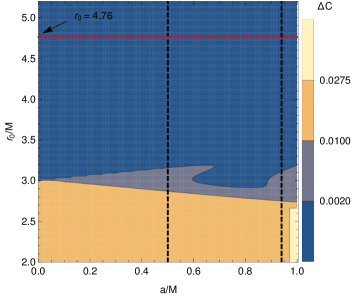
Figure 7: Dependence of the angular size and the deviation of the shadow on $r_{0}$ and spin. The region between the two black dashed vertical lines indicate the spin range $0.5\leq a_{*}\leq 0.94$. The horizontal red dashed line indicates the critical throat size $r_{0c}=4.76M$, below which both the size and deviation from circularity of the shadow is consistent with the M87^∗ results.

VI Concluding Remarks

In this paper, we have investigated the shadow of a rotating traversable wormhole and compared our results with those of Kerr black hole of same mass and spin. The results obtained here will have several implications in the study of shadow. The throat of a wormhole plays very crucial role in shadow formation. We have found that, for small spin and smaller wormhole throat size, the shadow of a wormhole mimics those of the black hole. However, with increasing either the spin or the throat size, the shadow of a wormhole start deviating from that of a black hole. Detection of such deviation may possibly indicate the presence of a wormhole. In section V, we have constrained the size and the spin of the wormhole, using the results from M87^∗ observation telescope . In Fig. 7, we have shown the average diameter and the deviation from circularity of the shadow for different values of the spin and the wormhole throat size, taking inclination angle to be $\theta_{o}=17^{\circ}$, which the jet axis makes with the line of sight. Note that, the spin lies within the range $0.5\leq a_{*}\leq 0.94$, where $a_{*}=a/M$, and the diameter of the shadow is always greater than the minimum allowed value of $9.5$. However, the diameter will be within the maximum allowed value $12.5$, if the wormhole throat size is restricted below some critical value $r_{0}\leq r_{0c}=4.76M$. Also, the deviation from circularity is always less than $2.75\%$, i.e., $\Delta C\leq 0.0275$ for the allowed throat size $r_{0}<r_{0c}=4.76M$ and spin range $0.5\leq a_{*}\leq 0.94$. In other words, the results obtained here indicate that a wormhole having reasonable spin or throat size, can be distinguished from a black hole through observations of their shadow. Also worth noting a recent paper by Gralla et al. Gralla in which the emission profile originating near a black hole has been discussed and the ”photon rings” surrounding the dark black hole shadow has been studied, including the implications of the recent M87* Event Horizon Telescope observations and mass measurement on it. Previous studies claimed that the observed emission will peak near the photon ring, but this paper suggested otherwise. Distinguishing between a ”photon ring” (light rays that complete at least $n=5/4$ orbits) and a ”lensing ring” (light rays that complete between $3/4$ and $5/4$ orbits); it showed that, for optically thin emission, ”photon ring” produced a sharp feature near the critical impact parameter but the peak is so narrow, and the brightness being logarithmic, it never makes a significant contribution to the observed flux. This interesting study may motivate future studies on the emission spectra of a accretion disk surrounding the wormhole described in this paper.

References

- (1) A. Einstein and N. Rosen, Phys. Rev. 48, 73 (1935).
- (2) M. Morris and K. Throne , American J. Phys. 56, 395 (1988 ).
- (3) J. A. Gonz´alez, F. S. Guzm´an, and O. Sarbach, Classical Quantum Gravity 26, 015010 (2009); ibid., 015011 (2009).
- (4) H. G. Elis, J. Math. Phys. (N.Y.) 14, 104 (1973). H.-a. Shinkai and S. A. Hayward, Phys. Rev. D 66, 044005 (2002).
- (5) M. Visser, Lorentzian Wormhole: from Einstein to Hawking , AIP Press (1995).
- (6) J.G. Cramer et al., Phys. Rev. D 51, 3117 (1995). arXiv:astro-ph/9606001v2.
- (7) S. Doeleman, J. Weintroub, A. E. E. Rogers, R. Plambeck, R. Freund, R. P. J. Tilanus, P. Friberg and L. M. Ziurys et al., Nature 455, 78 (2008) [arXiv:0809.2442 [astro-ph]].
- (8) A. E. Broderick, T. Johannsen, A. Loeb, and D. Psaltis, Astrophys.J., 784, 7 (2014).
- (9) J. L. Li, L. Guo and B. Zhang, A Giant Step: from Millito Micro-arcsecond Astrometry, Proceedings of the International Astronomical Union, IAU Symposium 248, 182 (2008); http://kvn-web.kasi.re.kr/; http://www.astro.sci.yamaguchi-u.ac.jp/jvn/,
- (10) A. Riazuelo, “Seeing relativity – I. Basics of a raytracing code in a Schwarzschild metric,” 2015.
- (11) K. Akiyama et al. [Event Horizon Telescope Collaboration], Astrophys. J. Lett. 875, L1 (2019).
- (12) Event Horizon Telescope Collaboration, Dimitrios Psaltis et. al. : Phys. Rev. Lett. 125 : 14, 141104 (2020).
- (13) S.I. Kruglov, Mod. Phys. Lett. A 35 : 35, 2050291 (2020).
- (14) H. Davoudiasl, P. B. Denton, Phys. Rev. Lett. 123, 021102, 2019
- (15) S. Vagnozzi, L Visinelli, Phys. Rev. D 100, 024020, 2019
- (16) J. L. Synge, Mon. Not. Roy. Astron. Soc. 131, no. 3, 463 (1966).
- (17) J. P. Luminet, Astron. Astrophys. 75, 228 (1979).
- (18) A. F. Zakharov, F. De Paolis, G. Ingrosso, and A. A. Nucita, Astron. Astrophys. 442, 795 (2005).
- (19) A. F. Zakharov, , Phys. Rev. D 90, 062007 (2014).
- (20) J. M. Bardeen, “Timelike and null geodesies in the Kerr metric,” in Proceedings, Ecole d’Ete de Physique Theorique: Les Astres Occlus, eds. C. Witt and B. Witt (Les Houches, France, 1973), p. 215-239.
- (21) H. Falcke, F. Melia, and E. Agol, Astrophys. J. 528, L13 (2000).
- (22) R. Takahashi, , Astrophys. J. 611, 996 (2004).
- (23) R. Takahashi and K. Y. Watarai, Mon. Not. R. Astron. Soc. 374, 1515 (2007).
- (24) A. F. Zakharov, A. A. Nucita, F. De Paolis, and G. Ingrosso, New Astron. 10, 479 (2005).
- (25) K. Hioki and K.-I. Maeda, Phys. Rev. D 80, 024042 (2009).
- (26) F. De Paolis, G. Ingrosso, A. A. Nucita, A. Qadir, and A. F. Zakharov, Gen. Relativ. Gravit. 43, 977 (2011).
- (27) K. Beckwith and C. Done, Mon. Not. R. Astron. Soc. 359, 1217 (2005).
- (28) A. E. Broderick and A. Loeb, Astrophys. J. 636, L109 (2006).
- (29) A. Yumoto, D. Nitta, T. Chiba, and N. Sugiyama, Phys. Rev. D 86, 103001 (2012).
- (30) J. O. Shipley and S. R. Dolan, Classical Quantum Gravity 33, 175001 (2016).
- (31) P. J. Young, Phys. Rev. D 14, 3281 (1976).
- (32) A. de Vries, Classical Quantum Gravity 17, 123 (2000).
- (33) R. Takahashi, Publ. Astron. Soc. Jpn. 57, 273 (2005).
- (34) P. V. P. Cunha, C. A. R. Herdeiro, E. Radu, and H. F. Runarsson, Phys. Rev. Lett. 115, 211102 (2015).
- (35) P. V. P. Cunha, C. A. R. Herdeiro, B. Kleihaus, J. Kunz, and E. Radu, Phys. Lett. B 768, 373 (2017).
- (36) P. V. P. Cunha and C. A. R. Herdeiro, Gen. Relativ. Gravit. 50, 42 (2018).
- (37) P. V. P. Cunha, C. A. R. Herdeiro, and M. J. Rodriguez, Phys. Rev. D 97, 084020 (2018).
- (38) K. Hioki and U. Miyamoto, Phys. Rev. D 78, 044007 (2008).
- (39) S. Dastan, R. Saffari, and S. Soroushfar, arXiv:1610.09477.
- (40) Z. Li and C. Bambi, , J. Cosmol. Astropart. Phys. 01, 041 (2014).
- (41) A. Abdujabbarov, M. Amir, B. Ahmedov, and S. G. Ghosh, Phys. Rev. D 93, 104004 (2016).
- (42) A. Abdujabbarov, F. Atamurotov, Y. Kucukakca, B. Ahmedov, and U. Camci, Astrophys. Space Sci. 344, 429 (2013).
- (43) A. A. Abdujabbarov, F. Atamurotov, N. Dadhich, B.J. Ahmedov, and Z. Stuchlik, Eur. Phys. J. C 75, 399 (2015).
- (44) A. Abdujabbarov, B. Toshmatov, Z. Stuchlik, and B. Ahmedov, Int. J. Mod. Phys. D 26, 1750051 (2017).
- (45) A. A. Abdujabbarov, L. Rezzolla, and B. J. Ahmedov, Mon. Not. R. Astron. Soc. 454, 2423 (2015).
- (46) M. Amir and S. G. Ghosh, Phys. Rev. D 94, 024054 (2016).
- (47) M. Amir, B. P. Singh, and S. G. Ghosh, Eur. Phys. J. C. 78, 399 (2018).
- (48) M. Sharif and S. Iftikhar, Eur. Phys. J. C 76, 630 (2016).
- (49) N. Tsukamoto, Phys.Rev. D 97, 064021 (2018).
- (50) A. Saha, M. Modumudi, and S. Gangopadhyay, arXiv:1802.03276.
- (51) S. W. Wei and Y. X. Liu, J. Cosmol. Astropart. Phys. 11, 063 (2013).
- (52) A. Grenzebach, V. Perlick, and C. Lammerzahl,Phys. Rev. D 89, 124004 (2014).
- (53) L. Amarilla and E. F. Eiroa, Phys. Rev. D 85, 064019 (2012).
- (54) L. Amarilla and E. F. Eiroa, Phys. Rev. D 87, 044057 (2013).
- (55) F. Atamurotov, A. Abdujabbarov, and B. Ahmedov, Astrophys. Space Sci. 348, 179 (2013).
- (56) F. Atamurotov, A. Abdujabbarov, and B. Ahmedov, Phys. Rev. D 88, 064004 (2013).
- (57) F. Atamurotov, B. Ahmedov, and A. Abdujabbarov, Phys. Rev. D 92, 084005 (2015).
- (58) M. Wang, S. Chen, and J. Jing, J. Cosmol. Astropart. Phys. 10, 051 (2017).
- (59) U. Papnoi, F. Atamurotov, S. G. Ghosh, and B. Ahmedov, Phys. Rev. D 90, 024073 (2014).
- (60) Z. Younsi, A. Zhidenko, L. Rezzolla, R. Konoplya and Y. Mizuno, Phys. Rev. D 94, 084025 (2016).
- (61) R. Shaikh, P. Kocherlakota, R. Narayan and P. S. Joshi, MNRAS 482, 52 (2019)
- (62) R. Shaikh, Phys. Rev. D 100, 024028 (2019)
- (63) M. Ghasemi-Nodehi, M. Azreg-Aïnou, K. Jusufi, M. Jamil: Phys.Rev.D 102, 104032 (2020).
- (64) S. Kala, Saurabh , H. Nandan, P. Sharma, Int.J.Mod.Phys.A 35 : 28, 2050177 (2020).
- (65) F. Long, S. Chen, M. Wang, J. Jing, Eur. Phys. J. C 80, 1180 (2020).
- (66) Yang Guo, Yan-Gang Miao, Phys. Rev. D 102 , 084057 (2020)
- (67) Hong Guo, Hang Liu, Xiao-Mei Kuang, Bin Wang: Phys.Rev.D 102, 124019 (2020)
- (68) V. Cardoso and P. Pani, Living Rev. Rel. 22, 4 (2019).
- (69) C. Bambi,Phys. Rev. D 87, 107501 (2013).
- (70) O. Sarbach and T. Zannias, AIP Conf. Proc. 1473, 223 (2012).
- (71) P. G. Nedkova, V. Tinchev, and S. S. Yazadjiev, Phys. Rev. D 88, 124019 (2013).
- (72) A. Abdujabbarov, B. Juraev, B. Ahmedov, and Z. Stuchlik, Astrophys. Space Sci. 361, 226 (2016).
- (73) T. Ohgami and N. Sakai, Phys. Rev. D 91, 124020 (2015).
- (74) F. Lamy, E. Gourgoulhon, T. Paumard and F. H. Vincent, Class. Quant. Grav. 35, 115009 (2018) [arXiv:1802.01635 [grqc]].
- (75) M. Azreg-Ainou, J. Cosmol. Astropart. Phys. 7, 37 (2015).
- (76) T. Ohgami and N. Sakai, Phys. Rev. D 94, 064071 (2016).
- (77) F. H. Vincent, M. Wielgus, M. A. Abramowicz, E. Gourgoulhon, J. P. Lasota, T. Paumard and G. Perrin, arXiv:2002.09226 [gr-qc].
- (78) M. Amir, K. Jusufi, A. Banerjee, S. Hansraj, Class. Quant .Grav. 36, 215007 (2019).
- (79) M. Amir, A. Banerjee, S. D. Maharaj : Annals Phys. 400, 198 (2019).
- (80) G. Gyulchev, P. Nedkova, V. Tinchev, S. Yazadjiev : Eur. Phys. J. C 78: 7, 544 (2018).
- (81) R. Shaikh: Phys. Rev. D 98, 024044 (2018).
- (82) A. Abdujabbarov, B. Juraev, B. Ahmedov, Z. Stuchlík, Astrophys. Space Sci. 361, 226 (2016).
- (83) M. Wielgus, J. Horak, F. Vincent, M. Abramowicz, Phys. Rev. D 102 : 8, 084044(2020).
- (84) R. Shaikh, P. Banerjee, S. Paul, and Tapobrata Sarkar, Phys. Lett. B 789, 270 (2019).
- (85) R. Shaikh, P. Banerjee, S. Paul and T. Sarkar, JCAP 07, 028 (2019).
- (86) N. Tsukamoto, arXiv: 2105.14336.
- (87) Xiaobao Wang, Peng-Cheng Li, Cheng-Yong Zhang, Minyong Guo : Phys.Lett.B 811, 135930 (2020) .
- (88) E. Teo, Phys. Rev. D 58, 024014 (1998).
- (89) R. A. Konoplya and A. Zhidenkob, JCAP 12, 043 (2016).
- (90) A. E. Vazquez and E. P. Esteban, Nuovo Cimento B 119, 489 (2004)
- (91) C. Bambi, K. Freese, S. Vagnozzi and L. Visinelli, Phys. Rev. D 100, 044057 (2019).
- (92) S. E. Gralla, D. E. Holz, R. M. Wald, Phys.Rev.D 100 2, 024018 (2019).