On the power of Sobolev tests for isotropy under local rotationally symmetric alternatives

Abstract

We consider one of the most classical problems in multivariate statistics, namely the problem of testing isotropy, or equivalently, the problem of testing uniformity on the unit hypersphere $\mathcal{S}^{p-1}$ of $\mathbb{R}^{p}$. Rather than restricting to tests that can detect specific types of alternatives only, we consider the broad class of Sobolev tests. While these tests are known to allow for omnibus testing of uniformity, their non-null behavior and consistency rates, unexpectedly, remain largely unexplored. To improve on this, we thoroughly study the local asymptotic powers of Sobolev tests under the most classical alternatives to uniformity, namely, under rotationally symmetric alternatives. We show in particular that the consistency rate of Sobolev tests does not only depend on the coefficients defining these tests but also on the derivatives of the underlying angular function at zero. For any Sobolev test and any rotationally symmetric alternative, we derive the consistency rate of the Sobolev test and determine the corresponding local asymptotic powers. We show that Sobolev tests with non-zero coefficients at odd (respectively, even) ranks only are blind (at any polynomial rate) to alternatives with angular functions whose $k$th-order derivatives at zero vanish for any $k$ odd (respectively, even). Our asymptotic analysis requires investigating the non-standard behavior of random Chebyshev polynomials (for $p=2$) and random Gegenbauer polynomials (for $p\geq 3$) in the vicinity of the uniform distribution on $\mathcal{S}^{p-1}$. Our non-standard asymptotic results are illustrated with Monte Carlo exercises.

Keywords: Consistency rates; Directional statistics; Invariance; Rotationally symmetric distributions; Tests of isotropy/uniformity.

1 Introduction

The present paper deals with one of the oldest problems in multivariate statistics, namely the problem of testing isotropy or, equivalently, of testing uniformity on the unit hypersphere $\mathcal{S}^{p-1}:=\{\mathbf{x}\in\mathbb{R}^{p}:\|\mathbf{x}\|^{2}=\mathbf{x}^{\prime}\mathbf{x}=1\}$ of $\mathbb{R}^{p}$, for $p\geq 2$. This problem, that can be traced back to Bernoulli, (1735), is one of the most fundamental problems in directional statistics and is still much considered nowadays. To cite only a few recent works, tests of uniformity in the context of noisy data were studied in Lacour and Pham Ngoc, (2014) and Kim et al., (2016). Tests in the high-dimensional context were considered in Cai and Jiang, (2012), Cai et al., (2013), and Cutting et al., (2017). Projection-based tests were proposed in Cuesta-Albertos et al., (2009) and García-Portugués et al., 2020a . Uniformity tests were used in García-Portugués et al., 2020b to construct tests for rotational symmetry. Inference for location in the vicinity of the uniformity case was considered in Paindaveine and Verdebout, (2017); Paindaveine and Verdebout, 2020a . We refer to García-Portugués and Verdebout, (2018) for a recent review of uniformity tests.

To be more specific, we consider the problem of testing the null hypothesis that a probability measure ${\rm P}$ over $\mathcal{S}^{p-1}$ coincides with the uniform probability measure on $\mathcal{S}^{p-1}$, on the basis of a random sample $\mathbf{U}_{1},\ldots,\mathbf{U}_{n}$ from ${\rm P}$. The most classical test for this problem is the Rayleigh, (1919) test, which rejects the null hypothesis at asymptotic level $\alpha$ when

$$np\|\bar{\mathbf{U}}\|^{2}>\chi_{p;1-\alpha}^{2},$$ (1)

where $\bar{\mathbf{U}}:=n^{-1}\sum_{i=1}^{n}\mathbf{U}_{i}$ is the sample average of the observations and $\chi_{\ell;\beta}^{2}$ denotes the order-$\beta$ (lower) quantile of the chi-square distribution with $\ell$ degrees of freedom. As explained in Mardia and Jupp, (1999), the Rayleigh test is the likelihood ratio test for testing uniformity within the von Mises–Fisher model characterized by densities on $\mathcal{S}^{p-1}$ (throughout, densities are with respect to the surface area measure on $\mathcal{S}^{p-1}$) proportional to $\mathbf{u}\mapsto\exp(\kappa\mathbf{u}^{\prime}\boldsymbol{\theta})$; here, $\boldsymbol{\theta}\in{\cal S}^{p-1}$ is a location parameter and $\kappa\geq 0$ is a concentration parameter (the larger the value of $\kappa$, the more the probability mass is concentrated about $\boldsymbol{\theta}$). Clearly, the Rayleigh test is designed to show power under alternatives for which ${\rm E}[\mathbf{U}_{1}]$ deviates from its null value (the zero $p$-vector), but it will be blind to other alternatives. In particular, it will be blind to (centro-)symmetric (or axial) alternatives. To detect such symmetric alternatives, first-order moments can be replaced with second-order ones, which leads to the Bingham, (1974) test rejecting the null hypothesis of uniformity at asymptotic level $\alpha$ when

$$\frac{np(p+2)}{2}{\rm tr}\Big{[}\Big{(}\mathbf{S}-\frac{1}{p}\mathbf{I}_{p}\Big{)}^{2}\Big{]}>\chi_{(p-1)(p+2)/2;1-\alpha}^{2},$$ (2)

where $\mathbf{I}_{p}$ is the $p$-dimensional identity matrix and $\mathbf{S}:=n^{-1}\sum_{i=1}^{n}\mathbf{U}_{i}\mathbf{U}_{i}^{\prime}$ is the empirical covariance matrix of the observations, relative to the fixed location vector zero.

The Rayleigh and Bingham tests have been extensively studied in the literature. In particular, Chikuse, (2003) showed that the Rayleigh test is a locally most powerful rotation-invariant test against von Mises–Fisher alternatives. Jupp, (2001) proposed modifications of the Rayleigh and Bingham tests to improve their asymptotic chi-square approximations. Cutting et al., (2017) established that the Rayleigh test detects local von Mises–Fisher alternatives in $\kappa_{n}\sim p_{n}^{3/4}/\sqrt{n}$ in the high-dimensional case. The Bingham test is the likelihood ratio test for testing uniformity against the alternatives associated with the Bingham, (1974) distributions or the angular Gaussian distributions from Tyler, (1987). Cutting et al., (2020) derived the local powers of the Bingham test under rotationally symmetric alternatives. The consistency rate of this test in high dimensions was also recently obtained in Cutting et al., (2021). Finally, note that the Rayleigh and Bingham tests can be seen as the spatial sign test for location and for sphericity, respectively; see Hallin and Paindaveine, (2002) and Hallin and Paindaveine, (2006), respectively.

The Rayleigh and Bingham tests actually belong to the class of Sobolev tests introduced in Beran, (1968, 1969); see also Giné, (1975). Sobolev tests reject the null hypothesis of uniformity for large values of

$$S^{(n)}_{v}:=\frac{1}{n}\sum_{i,j=1}^{n}\sum_{k=1}^{\infty}v_{k}^{2}h_{p,k}(\mathbf{U}_{i}^{\prime}\mathbf{U}_{j}),$$ (3)

where $h_{p,k}(s):=(2\mathbb{I}[p=2]+\big{(}1+\frac{2k}{p-2}\big{)}\mathbb{I}[p\geq 3])C_{k}^{(p-2)/2}(s)$, $s\in[-1,1]$, involves Chebyshev polynomials of the first kind $C_{k}^{0}$ for $p=2$ and Gegenbauer polynomials $C_{k}^{\lambda}$, $\lambda>0$, for $p\geq 3$; see Section 2 for a definition of these polynomials, for the construction of Sobolev tests, and for the summability condition the sequence of coefficients $v=(v_{k})$ should obviously satisfy. The Rayleigh and Bingham tests are obtained by taking $v_{k}=\delta_{k1}$ and $v_{k}=\delta_{k2}$, where $\delta_{k\ell}$ is the usual Kronecker delta. Many further Sobolev tests, associated with other sequences $v$, have been considered in the literature; among them, the Watson, (1961) and Ajne, (1968) tests of uniformity on $\mathcal{S}^{1}$, the tests considered in Giné, (1975), Prentice, (1978), Pycke, (2007, 2010) and Jammalamadaka et al., (2020), as well as the data-driven Sobolev tests proposed in Bogdan et al., (2002) and Jupp, (2008). The Bayesian optimality of Sobolev tests has recently been studied in Sun and Lockhart, (2019). We refer to García-Portugués and Verdebout, (2018) for an overview of the various Sobolev tests that have been considered in the literature.

While the asymptotic behavior of Sobolev tests has been well studied under the null hypothesis of uniformity, little is known about their non-null limiting behavior. Precisely, it is well-known that, provided that $v_{k}\neq 0$ for any $k$, Sobolev tests are universally consistent, that is, are consistent under any fixed alternative to uniformity; see Theorem 4.4 in Giné, (1975). But limiting non-trivial powers under general local alternatives—or even simply consistency rates—remain to be thoroughly explored. The objective of this paper is to fill this gap. More precisely, our goal is to provide an extensive study of the local asymptotic behavior of Sobolev tests under the most commonly considered alternatives to uniformity, namely under (absolutely continuous) rotationally symmetric ones. In other words, we consider alternatives associated with densities of the form

$$\mathbf{u}\mapsto c_{p,\kappa,f}f(\kappa\mathbf{u}^{\prime}\boldsymbol{\theta}),$$ (4)

where $\boldsymbol{\theta}\in\mathcal{S}^{p-1}$ is a location parameter, $\kappa>0$ is a concentration parameter, $f:\mathbb{R}\to\mathbb{R}^{+}$ is an angular function with $f(0)=1$ (for standardization), and

$$c_{p,\kappa,f}:=1\,\Big{/}\int_{-1}^{1}(1-s^{2})^{(p-3)/2}f(\kappa s)\,\mathrm{d}s$$ (5)

is a normalizing constant. These parameters are not identified (the concentration parameter $\kappa$ may always be included in $f$; also, when $f$ is symmetric about zero, $\boldsymbol{\theta}$ is only identified up to a sign), but this will not be an issue in the sequel since these distributions are only providing alternatives under which to investigate the asymptotic properties of perfectly well-defined tests. Many well-known distributions on the sphere fit in the setup of (4). For instance, the von Mises–Fisher distributions introduced above, that are often regarded as the $\mathcal{S}^{p-1}$-equivalent of Gaussian distributions on ${\mathbb{R}}^{p}$, are obtained with $f(s)=\exp(s)$. Watson distributions (Watson,, 1965), that are associated with $f(s)=\exp(s^{2})$, provide a single-spiked version of the Bingham, (1974) distributions. Further distributions of this type are the directional Cauchy distributions with angular function $f(s)=(1+2s)^{-1}$ (García-Portugués,, 2013) and the exponential distributions with angular functions $f(s)=\exp(s^{b})$ for $b>0$ (Paindaveine and Verdebout, 2020b, ), as well as other distributions that can be reparametrized to fit (4) (see, e.g., McCullagh, 1989, Jones and Pewsey, 2005, or Kato and McCullagh, 2020). In the present paper, we investigate the limiting behavior of Sobolev tests under local alternatives of the form (4), that is, when $\kappa$ is replaced in (4) with a sequence $(\kappa_{n})$ converging to zero at a suitable rate.

Our results reveal that a Sobolev test typically shows non-trivial asymptotic powers against alternatives in $\kappa_{n}\sim n^{-1/(2k_{v})}$, where $k_{v}$ is the rank of the first non-zero coefficient in the sequence $v=(v_{k})$. More precisely, this is the case if $f^{\underline{k_{v}}}(0)\neq 0$ (henceforth, $f^{\underline{k}}$ stands for the $k$th derivative of $f$). If this derivative is equal to zero, then slower consistency rates are achieved. Therefore, consistency rates of Sobolev tests do not only depend on the particular test used (that is, on the sequence $v$) but also on which derivatives $f^{\underline{k}}(0)$ are equal to zero. In the case where $f^{\underline{k_{v}}}(0)=0$, we determine the local alternatives (if any) that can be detected by a Sobolev test. Remarkably, parity of the ranks $k$ for which $v_{k}$ and $f^{\underline{k}}(0)$ are non-zero plays a key role in the resulting consistency rates. In particular, we establish that Sobolev tests with non-zero coefficients $v_{k}$ at odd (resp., even) ranks only are blind (at any polynomial rate) to alternatives such that with $f^{\underline{k}}(0)=0$ for any $k$ odd (resp., even). The subtle nature of our asymptotic results prevent us from being more specific in this introduction. Let us still mention, however, that whenever we identify in the sequel the consistency rate of a Sobolev test, we will provide the exact expression of the corresponding limiting non-trivial powers.

The paper is organized as follows. In Section 2, we first introduce the mathematical objects (including spherical harmonics as well as Chebyshev and Gegenbauer polynomials) that are needed to define Sobolev tests. We then recall what is known on the asymptotic null behavior of these tests. In Section 3, we study how the first moments of spherical harmonics evaluated at observations behave in the vicinity of uniformity, which requires investigating first moments of random Chebyshev and Gegenbauer polynomials. While the results of Section 3 are of independent interest, we exploit them in this paper to identify the consistency rates of Sobolev tests and to derive the corresponding local asymptotic powers; this is done in Section 4 and in Section 5, for finite and infinite Sobolev tests, respectively (we say that a Sobolev test is finite if and only if finitely many of its coefficients $v_{k}$ are non-zero). In Section 6, we conduct several Monte Carlo exercises in order to illustrate the non-null results obtained in the previous sections. Finally, we briefly discuss perspectives for future research in Section 7. All proofs are provided in the appendix.

For convenience, we collect here some notation that will be used in the sequel. We will denote as ${\bf e}_{\ell,k}$ the $\ell$th vector of the canonical basis of $\mathbb{R}^{k}$. To make the notation lighter, we will simply write ${\bf e}_{\ell}$ whenever the dimension of the ambient Euclidean space can be recovered from the mathematical objects involved in the various formulae. We will denote as $\nu_{p}$ the uniform probability measure on $\mathcal{S}^{p-1}$, that is, $\sigma_{p}/\omega_{p-1}$, where $\sigma_{p}$ is the surface area measure on $\mathcal{S}^{p-1}$ and $\omega_{p-1}=\sigma_{p}(\mathcal{S}^{p-1})=2\pi^{p/2}/\Gamma(p/2)$ is the surface area of $\mathcal{S}^{p-1}$. This allows us to consider the inner product $\langle f,g\rangle:=\int_{\mathcal{S}^{p-1}}f(\mathbf{x})g(\mathbf{x})\,\mathrm{d}\nu_{p}(\mathbf{x})$ on $L^{2}(\mathcal{S}^{p-1},\nu_{p})$. For a real number $a$ and a nonnegative integer $k$, we will use the Pochhammer symbol $(a)_{k}:=a(a+1)\cdots(a+k-1)$ for $k>0$ and $(a)_{k}:=1$ for $k=0$. The relation $k\sim\ell$ on $\mathbb{N}$ is satisfied when $k$ and $\ell$ share the same parity. We will write ${\rm diag}({\bf B}_{1},\ldots,{\bf B}_{\ell})$ for the block-diagonal matrix with diagonal blocks ${\bf B}_{1},\ldots,{\bf B}_{\ell}$. Weak convergence will be denoted as $\stackrel{{\scriptstyle\mathcal{D}}}{{\to}}$. Finally,

$$c_{p}:=\frac{\Gamma(\frac{p}{2})}{\sqrt{\pi}\Gamma(\frac{p-1}{2})}$$ (6)

will be the value of the normalizing constant (5) that is obtained in the uniform case (that is, $c_{p}=c_{p,0,f}$, irrespective of $f$).

2 Spherical harmonics and Sobolev tests

Sobolev tests on $\mathcal{S}^{p-1}$ are constructed via an orthonormal basis of $L^{2}(\mathcal{S}^{p-1},\nu_{p})$ associated with spherical harmonics. In this section, we first briefly present spherical harmonics, then we explain how they lead to Sobolev tests, and finally we review what is known on the asymptotic null behavior of these tests.

Fix an integer $p\geq 2$ and a nonnegative integer $k$. Denote as $\mathcal{P}^{p}_{k}$ the space of real homogeneous polynomials of degree $k$ and as $\mathcal{H}^{p}_{k}$ the linear subspace of $\mathcal{P}^{p}_{k}$ collecting polynomials whose Laplacian is zero. Spherical harmonics of degree $k$ simply are the restrictions to $\mathcal{S}^{p-1}$ of polynomials in $\mathcal{H}^{p}_{k}$. In the sequel, we will also denote as $\mathcal{H}^{p}_{k}$ the collection of spherical harmonics of degree $k$. It is well-known that $\mathcal{H}^{p}_{k}$ is a vector space with dimension

$${\textstyle{d_{p,k}=\binom{p+k-1}{k}-\binom{p+k-3}{k-2}=\binom{p+k-3}{p-2}+\binom{p+k-2}{p-2};}}$$

see, e.g., Corollary 1.1.4 in Dai and Xu, (2013). Spherical harmonics associated with different values of $k$ are orthogonal: if $\varphi\in\mathcal{H}^{p}_{k}$ and $\psi\in\mathcal{H}^{p}_{\ell}$ with $k\neq\ell$, then $\langle\varphi,\psi\rangle=0$. Therefore, merging orthonormal bases of several harmonic spaces $\mathcal{H}^{p}_{k}$ provides an orthonormal basis of the direct sum of these spaces. Moreover, the collection of all spherical harmonics is dense in $L^{2}(\mathcal{S}^{p-1},\nu_{p})$, which coincides with the direct sum of $\mathcal{H}^{p}_{k}$, $k=0,1,\ldots$; see, e.g., Theorem 2.2.2 in Dai and Xu, (2013).

For each value of $k$, we now provide a specific orthonormal basis of $\mathcal{H}^{p}_{k}$ that is convenient for computations. For $k=0$, we have $d_{p,0}=1$ and a corresponding basis of $\mathcal{H}^{p}_{k}$ is $\{g_{1,0}\}$, with $g_{1,0}(\mathbf{x})=1$ for any $\mathbf{x}$. We may therefore restrict to positive values of $k$. For $p=2$, we have $d_{2,k}=2$ for any positive integer $k$, and the functions that are defined using polar coordinates $\mathbf{x}=(x_{1},x_{2})^{\prime}=(\sin\theta,\cos\theta)^{\prime}\in\mathcal{S}^{1}$ (with $0\leq\theta<2\pi$) through

$$g_{1,k}(\mathbf{x})=\sqrt{2}\cos(k\theta)\quad\textrm{ and }\quad g_{2,k}(\mathbf{x})=\sqrt{2}\sin(k\theta)$$ (7)

form an orthonormal basis of $\mathcal{H}^{p}_{k}$. The case $p\geq 3$ is substantially more intricate. Consider the hyperspherical coordinates where $\mathbf{x}=(x_{1},\ldots,x_{p})^{\prime}\in\mathcal{S}^{p-1}$ writes

$$\left\{\!\begin{array}[]{rl}x_{1}=&\!\!\!\sin\theta_{p-1}\cdots\sin\theta_{2}\sin\theta_{1},\\ x_{2}=&\!\!\!\sin\theta_{p-1}\cdots\sin\theta_{2}\cos\theta_{1},\\ &\vdots\\ x_{p-1}=&\!\!\!\sin\theta_{p-1}\cos\theta_{p-2},\\ x_{p}=&\!\!\!\cos\theta_{p-1},\end{array}\right.$$

with $0\leq\theta_{1}<2\pi$, and $0\leq\theta_{j}\leq\pi$ for $j=2,\ldots,p-1$. Let further $C_{q}^{\lambda}$ be the Gegenbauer polynomial of degree $q$, defined for any $\lambda>0$ and $q\in\mathbb{N}_{0}$, through

$$C_{q}^{\lambda}(t):=\frac{(\lambda)_{q}2^{q}}{q!}t^{q}\,{}_{2}F_{1}({\textstyle{-\frac{q}{2},\frac{1-q}{2};1-q-\lambda;\frac{1}{t^{2}}}})=\sum_{j=0}^{\lfloor q/2\rfloor}(-1)^{j}c^{\lambda}_{q,j}t^{q-2j},$$ (8)

where ${}_{2}F_{1}$ is the hypergeometric function and where

$$c^{\lambda}_{q,j}:=\frac{2^{q-2j}\Gamma(q-j+\lambda)}{\Gamma(\lambda)j!(q-2j)!}\cdot$$

For $p=3$, Gegenbauer polynomials reduce to Legendre polynomials. In the sequel, we will also need to consider the Chebyshev polynomial of the first kind with degree $q$, which is defined through $C_{q}^{0}(\cos\theta):=\cos(q\theta)$, hence is given by

$$C_{q}^{0}(t)=\sum_{j=0}^{\lfloor q/2\rfloor}(-1)^{j}c^{0}_{q,j}t^{q-2j},\ \ \textrm{with }\ c^{0}_{q,j}:=\frac{2^{q-2j-1}q\Gamma(q-j)}{j!(q-2j)!}\cdot$$ (9)

Chebyshev and Gegenbauer polynomials are connected by $\lim_{\lambda\to 0}\lambda^{-1}C_{k}^{\lambda}(s)=(2/k)C_{k}^{0}(s)$, $s\in[-1,1]$. The following result provides an orthonormal basis of $\mathcal{H}^{p}_{k}$ for $p\geq 3$ and $k>0$; see Theorem 1.5.1 in Dai and Xu, (2013). The proposition incorporates corrections to several errata present in the statement of Theorem 1.5.1.

Proposition 1.

Fix an integer $p\geq 3$ and a positive integer $k$. Let $\mathcal{M}_{k}=\{{\bf m}\in\mathbb{N}_{0}^{p}:|{\bf m}|:=m_{1}+\cdots+m_{p}=k\textrm{ and }m_{p}\in\{0,1\}\}$. For any ${\bf m}\in\mathcal{M}_{k}$, let

$$\zeta_{\bf m}(s):=\begin{cases}\cos(m_{p-1}s)&\textrm{if }m_{p}=0,\\ \sin((m_{p-1}+1)s)&\textrm{if }m_{p}=1,\end{cases}$$

and

$$B_{\bf m}:=b_{\bf m}\prod_{j=1}^{p-2}\frac{m_{j}!(\frac{p-j+1}{2})_{|m^{j+1}|}(m_{j}+\lambda_{j})}{(2\lambda_{j})_{m_{j}}(\frac{p-j}{2})_{|m^{j+1}|}\lambda_{j}},$$

where we write $|{\bf m}^{j}|=m_{j}+\cdots+m_{p}$ and $\lambda_{j}:=|m^{j+1}|+(p-j-1)/2$ for any $j=1,\ldots,p-2$, and where $b_{\bf m}:=2$ if $m_{p-1}+m_{p}>0$ and $b_{\bf m}:=1$ otherwise. Then, defining $\varphi_{\bf m}:\mathcal{S}^{p-1}\to\mathbb{R}$ in spherical coordinates through

$$\varphi_{\bf m}(\mathbf{x}):=\sqrt{B_{\bf m}}\,\zeta_{\bf m}(\theta_{1})\prod_{j=1}^{p-2}(\sin\theta_{p-j})^{|{\bf m}^{j+1}|}C_{m_{j}}^{\lambda_{j}}(\cos\theta_{p-j}),$$ (10)

the collection $\{\varphi_{\bf m}:{\bf m}\in\mathcal{M}_{k}\}$ is a real orthonormal basis of $\mathcal{H}^{p}_{k}$, in the sense that $\langle\varphi_{\bf m},\varphi_{\bf m^{\prime}}\rangle=\delta_{{\bf m},{\bf m}^{\prime}}$ for any ${\bf m},{\bf m}^{\prime}\in\mathcal{M}_{k}$.

Note that this orthonormal basis is indeed of cardinality $d_{p,k}$. To work with a specific basis in the rest of the paper, we adopt the following notation. Let us enumerate the ${\bf m}$’s in $\mathcal{M}_{k}$ as ${\bf m}_{r}$, $r=1,\ldots,d_{p,k}$, in an arbitrary way but for the fact that ${\bf m}_{1}=(k,0,\ldots,0)$ (the exact ordering for $r=2,\ldots,d_{p,k}$ will not be important in the sequel). We then let

$$g_{1,k}(\mathbf{x}) =\varphi_{{\bf m}_{1}}(\mathbf{x})=\frac{1}{\sqrt{d_{p,k}}}\Big{(}1+\frac{2k}{p-2}\Big{)}C_{k}^{(p-2)/2}(\cos\theta_{p-1}),$$ (11)

$$g_{r,k}(\mathbf{x}) =\varphi_{{\bf m}_{r}}(\mathbf{x}),\quad r=2,\ldots,d_{p,k}.$$ (12)

As shown in the later sections, $g_{1,k}$ is the only basis function of $\mathcal{H}^{p}_{k}$ that will play an essential role in the paper. The exact expression of the remaining basis functions in (12), which is rather cumbersome (see (10)), will play a very minor role only.

Irrespective of $p$, one has the addition formula

$$\sum_{r=1}^{d_{p,k}}g_{r,k}(\mathbf{u})g_{r,k}(\mathbf{v})=\begin{cases}2\cos(k\angle(\mathbf{u},\mathbf{v}))=2C_{k}^{0}(\mathbf{u}^{\prime}\mathbf{v})&{\rm for}\;p=2,\\ \big{(}1+\frac{2k}{p-2}\big{)}C_{k}^{(p-2)/2}({\bf u}^{\prime}\mathbf{v})&{\rm for}\;p\geq 3,\end{cases}$$ (13)

where $\angle(\mathbf{u},\mathbf{v}):=\arccos(\mathbf{u}^{\prime}\mathbf{v})$ is the angle between $\mathbf{u},\mathbf{v}\in\mathcal{S}^{p-1}$; see Equation (1.2.8) in Dai and Xu, (2013) for $p\geq 3$. The name follows from the fact that this result extends to $p\geq 3$ what is the usual addition formula of the cosine function for $p=2$.

Now, for any real sequence $v=(v_{k})$ such that $\sum_{k=1}^{\infty}v_{k}^{2}d_{p,k}<\infty$, consider the mapping ${\rm t}:\mathcal{S}^{p-1}\to L^{2}(\mathcal{S}^{p-1},\nu_{p})$ that maps $\mathbf{u}$ to ${\rm t}(\mathbf{u}):=\sum_{k=1}^{\infty}v_{k}{\rm t}_{k}(\mathbf{u})$, where we let ${\rm t}_{k}(\mathbf{u}):=\sum_{r=1}^{d_{p,k}}g_{r,k}(\mathbf{u})g_{r,k}$ for any $\mathbf{u}\in\mathcal{S}^{p-1}$; see (7) for $p=2$ and the discussion below Proposition 1 for $p\geq 3$. Considering the mapping ${\bf G}_{p,k}:\mathcal{S}^{p-1}\to\mathbb{R}^{d_{p,k}}$ defined as ${\bf G}_{p,k}:=(g_{1,k},\ldots,g_{d_{p,k},k})^{\prime}$ allows us to formally define the Sobolev statistic

$$S^{(n)}_{v}:= \;\frac{1}{n}\sum_{i,j=1}^{n}\langle{\rm t}(\mathbf{U}_{i}),{\rm t}(\mathbf{U}_{j})\rangle=\frac{1}{n}\sum_{i,j=1}^{n}\sum_{k=1}^{\infty}v_{k}^{2}\langle{\rm t}_{k}(\mathbf{U}_{i}),{\rm t}_{k}(\mathbf{U}_{j})\rangle$$

$$= \;\frac{1}{n}\sum_{i,j=1}^{n}\sum_{k=1}^{\infty}v_{k}^{2}\bigg{(}\sum_{r=1}^{d_{p,k}}g_{r,k}(\mathbf{U}_{i})g_{r,k}(\mathbf{U}_{j})\bigg{)}=\sum_{k=1}^{\infty}v_{k}^{2}\bigg{\|}\frac{1}{\sqrt{n}}\sum_{i=1}^{n}{\bf G}_{p,k}(\mathbf{U}_{i})\bigg{\|}^{2},\!\!\!\!$$ (14)

where we used the fact that, for any $\mathbf{u},\mathbf{v}\in\mathcal{S}^{p-1}$, we have $\langle{\rm t}_{k}(\mathbf{u}),\allowbreak{\rm t}_{\ell}(\mathbf{v})\rangle=0$ for $k\neq\ell$ and $\langle{\rm t}_{k}(\mathbf{u}),{\rm t}_{k}(\mathbf{v})\rangle=\sum_{r=1}^{d_{p,k}}g_{r,k}(\mathbf{u})g_{r,k}(\mathbf{v})=({\bf G}_{p,k}(\mathbf{u}))^{\prime}{\bf G}_{p,k}(\mathbf{v})$. The addition formula above now allows us to write $S^{(n)}_{v}$ as in (3), which is the formula that is used in practice to evaluate this test statistic. Since the expression of $S^{(n)}_{v}$ in (3) involves the observations $\mathbf{U}_{i}$, $i=1,\ldots,n$, only through the inner products $\mathbf{U}_{i}^{\prime}\mathbf{U}_{j}$, Sobolev tests are rotation-invariant in the sense that $S^{(n)}_{v}(\mathbf{O}\mathbf{U}_{1},\ldots,\mathbf{O}\mathbf{U}_{n})=S^{(n)}_{v}(\mathbf{U}_{1},\ldots,\mathbf{U}_{n})$ for any $p\times p$ orthogonal matrix $\mathbf{O}$.

We now describe the asymptotic null behavior of Sobolev test statistics. Write ${\rm P}_{0}^{(n)}$ for the hypothesis under which the observations $\mathbf{U}_{1},\ldots,\mathbf{U}_{n}$ form a random sample from the uniform distribution on $\mathcal{S}^{p-1}$. Throughout, expectations and variances under ${\rm P}_{0}^{(n)}$ will be denoted as ${\rm E}_{0}^{(n)}[\cdot]$ and ${\rm Var}_{0}^{(n)}[\cdot]$, respectively. Assume for a moment that the Sobolev test statistic $S^{(n)}_{v}$ is finite, with $K_{v}:=\max\{k:v_{k}\neq 0\}$ say. Then, the last expression in (14) entails that

$$S^{(n)}_{v}=n({\bf T}_{p,K_{v}}^{(n)})^{\prime}{\rm diag}(v_{1}^{2}{\bf I}_{d_{p,1}},\ldots,v_{K_{v}}^{2}{\bf I}_{d_{p,K_{v}}}){\bf T}_{p,K_{v}}^{(n)},$$ (15)

with

$${\bf T}_{p,K}^{(n)}:=\frac{1}{n}\sum_{i=1}^{n}\left(({\bf G}_{p,1}(\mathbf{U}_{i}))^{\prime},\ldots,({\bf G}_{p,K}(\mathbf{U}_{i}))^{\prime}\right)^{\prime}.$$

For any positive integer $k$, orthonormality of the functions ${g}_{r,k}$, $r=1,\ldots,d_{p,k}$ and mutual orthogonality of the subspaces $\mathcal{H}^{p}_{k}$, $k=0,1,\ldots$, entail that

$${\rm E}_{0}^{(n)}[{\bf G}_{p,k}(\mathbf{U}_{1})] ={\bf 0},$$ (16)

$${\rm Var}_{0}^{(n)}[{\bf G}_{p,k}(\mathbf{U}_{1})] ={\bf I}_{d_{p,k}},$$ (17)

and

$${\rm E}_{0}^{(n)}[{\bf G}_{p,k}(\mathbf{U}_{1})({\bf G}_{p,\ell}(\mathbf{U}_{1}))^{\prime}]={\bf 0},\quad k\neq\ell.$$ (18)

The central limit theorem therefore readily implies that $S^{(n)}_{v}$ converges weakly under ${\rm P}_{0}^{(n)}$ to $\sum_{k=1}^{K_{v}}v_{k}^{2}Y_{k}$, where the random variables $Y_{k}$ are mutually independent and satisfy $Y_{k}\sim\chi^{2}_{d_{p,k}}$ for any $k$. The result actually extends to infinite Sobolev tests, under the summability condition provided in the following theorem; see Theorem 4.1 and Equation (4.2) in Giné, (1975).

Theorem 1.

Fix an integer $p\geq 2$ and a sequence $v=(v_{k})$ such that $\sum_{k=1}^{\infty}v_{k}^{2}d_{p,k}<\infty$. Then, under ${\rm P}^{(n)}_{0}$,

$$S^{(n)}_{v}\stackrel{{\scriptstyle\mathcal{D}}}{{\to}}\sum_{k=1}^{\infty}v_{k}^{2}Y_{k}$$

as $n$ diverges to infinity, where the random variables $Y_{k}$ are mutually independent and satisfy $Y_{k}\sim\chi^{2}_{d_{p,k}}$ for any $k$.

Obviously, the resulting infinite Sobolev tests reject the null hypothesis of uniformity at asymptotic level $\alpha$ when $S^{(n)}_{v}$ exceeds the upper $\alpha$-quantile of the distribution of $\sum_{k=1}^{\infty}v_{k}^{2}Y_{k}$.

3 Non-null moments of random spherical harmonics

The main objective of this paper is to study the asymptotic behavior of a generic Sobolev test under suitable local versions of the alternatives described in the introduction. Accordingly, write ${\rm P}_{\boldsymbol{\theta},\kappa_{n},f}^{(n)}$ for the hypothesis under which the observations $\mathbf{U}_{1},\ldots,\mathbf{U}_{n}$ form a random sample from a rotationally symmetric distribution with location $\boldsymbol{\theta}$, concentration $\kappa_{n}$, and angular function $f$; see (4). From rotation-invariance, the power of Sobolev tests under ${\rm P}_{\boldsymbol{\theta},\kappa_{n},f}^{(n)}$ will not depend on $\boldsymbol{\theta}$, so we may safely restrict in the sequel to the case $\boldsymbol{\theta}=\boldsymbol{\theta}_{0}=(0,\ldots,0,1)^{\prime}\in\mathbb{R}^{p}$. The resulting sequence of hypotheses will be denoted as ${\rm P}_{\kappa_{n},f}^{(n)}$, and the corresponding expectation and variance will be denoted as ${\rm E}_{\kappa_{n},f}^{(n)}[\cdot]$ and ${\rm Var}^{(n)}_{\kappa_{n},f}[\cdot]$, respectively.

The discussion at the end of the previous section makes it clear that the asymptotic non-null behavior of Sobolev tests will be governed by the non-null counterparts of (16)–(18). We have the following result.

Proposition 2.

Fix an integer $p\geq 2$ and a positive integer $k$. Let $(\kappa_{n})$ be a positive real sequence that is $o(1)$ and $f$ be an angular function that is continuous at zero. Then, as $n$ diverges to infinity,

$${\rm E}^{(n)}_{\kappa_{n},f}[{\bf G}_{p,k}(\mathbf{U}_{1})] =t_{p,k}\,\mathrm{E}_{\kappa_{n},f}^{(n)}\big{[}C_{k}^{(p-2)/2}(\mathbf{U}_{1}^{\prime}\boldsymbol{\theta}_{0})\big{]}{\bf e}_{1},$$ (19)

$${\rm Var}_{\kappa_{n},f}^{(n)}[{\bf G}_{p,k}(\mathbf{U}_{1})] ={\bf I}_{d_{p,k}}+o(1),$$ (20)

and

$${\rm E}_{\kappa_{n},f}^{(n)}[{\bf G}_{p,k}(\mathbf{U}_{1})({\bf G}_{p,\ell}(\mathbf{U}_{1}))^{\prime}]=o(1),\quad k\neq\ell,$$ (21)

with $t_{p,k}:=\sqrt{2}$ for $p=2$ and $t_{p,k}:=(1+2k/(p-2))/\sqrt{d_{p,k}}$ for $p\geq 3$.

Comparing (19)–(21) with (16)–(18), this result shows that the behavior of Sobolev tests under local alternatives will be exclusively conducted by the shift the expectations in (19) show compared to the null hypothesis. In order to derive the corresponding limiting powers, we need to describe the way the expectation in the right hand side of (19) behaves as a function of $\kappa_{n}$. Now, this expectation involves Chebyshev polynomials (for $p=2$) or Gengenbauer polynomials (for $p\geq 3$), hence in all cases can be decomposed in terms of the non-null moments $e_{n,m}:={\rm E}^{(n)}_{\kappa_{n},f}[(\mathbf{U}_{1}^{\prime}\boldsymbol{\theta}_{0})^{m}]$, $m=0,1,\ldots$ We recall that the corresponding null moments are given by

$$a_{m}:= \;{\rm E}^{(n)}_{0}[(\mathbf{U}_{1}^{\prime}\boldsymbol{\theta}_{0})^{m}]=c_{p}\int_{-1}^{1}s^{m}(1-s^{2})^{(p-3)/2}\,\mathrm{d}s$$

$$= \;\mathbb{I}[{\textstyle{\frac{m}{2}}}\in{\mathbb{N}}]\frac{\Gamma(\frac{m+1}{2})\Gamma(\frac{p}{2})}{\sqrt{\pi}\Gamma(\frac{m+p}{2})}=\mathbb{I}[{\textstyle{\frac{m}{2}}}\in{\mathbb{N}}]\prod_{r=0}^{{\textstyle{\frac{m}{2}}}-1}\frac{1+2r}{p+2r},\quad m=0,1,\ldots,$$ (22)

with the convention that a product involving no factor is equal to one; see, e.g., Lemma A.1 in Paindaveine and Verdebout, (2016). The next result then describes how the non-null moments $e_{n,m}$ behave in terms of $\kappa_{n}$.

Proposition 3.

Fix an integer $p\geq 2$ and integers $q\geq m>0$. Let $(\kappa_{n})$ be a positive real sequence that is $o(1)$ and $f$ be an angular function that is $q-m$ times differentiable at zero. Define the coefficients $b_{m,i}$ through

$$(b_{m,0},b_{m,1},\ldots,b_{m,q-m})^{\prime}:=\mathbf{A}_{q-m}^{-1}\mathbf{v}_{q-m}^{(m)},$$

where the $(t+1)\times(t+1)$ matrix $\mathbf{A}_{t}$ and $(t+1)$-vector $\mathbf{v}_{t}^{(m)}$ are defined as

$$\mathbf{A}_{t}=\bigg{(}a_{i-j}\frac{f^{\underline{i-j}}(0)}{(i-j)!}\mathbb{I}[i\geq j]\bigg{)}_{i,j=0,1,\ldots,t}\textrm{ and }\ \mathbf{v}_{t}^{(m)}=\bigg{(}a_{m+i}\frac{f^{\underline{i}}(0)}{i!}\bigg{)}_{i=0,1,\ldots,t}.$$

Then,

$$e_{n,m}=\sum_{\ell=0}^{q-m}b_{m,\ell}\kappa_{n}^{\ell}+o({\kappa_{n}^{q-m}})$$

as $n$ diverges to infinity.

This result, that is of independent interest, is an important step to derive the asymptotic behavior of the expectation in the righthand side of (19). To state the result, we need the following further notation. For any positive integer $i$, define the coefficients $m_{k,i}$, $k=0,1,\ldots,i$, through

$$\sum_{k=0}^{i}m_{k,i}C_{k}^{(p-2)/2}(t)=t^{i}.$$ (23)

These coefficients are uniquely defined since the polynomials $C_{k}^{(p-2)/2}$, $k=0,1,\ldots,i$, form a basis of the vector space of polynomials of degree at most $i$. Note that, irrespective of $i$, we have $m_{i-\ell,i}=0$ for $\ell$ odd (see Equation (2.29) in Wünsche,, 2017), so that a necessary condition for $m_{k,i}\neq 0$ is that $k\sim i$ (recall that this means that $k$ and $i$ have the same parity). We then have the following result.

Proposition 4.

Fix integers $p\geq 2$, $k>0$, and $r\geq 0$. Let $(\kappa_{n})$ be a positive real sequence that is $o(1)$ and $f$ be an angular function that is $k+r$ times differentiable at zero. Let ${\bf z}^{(k)}_{t}$ be the $(t+1)$-vector

$${\bf z}_{t}^{(k)}=\bigg{(}\frac{m_{k,i}f^{\underline{i}}(0)}{i!}\mathbb{I}[k\leq i]\bigg{)}_{i=0,1,\ldots,t}$$

and ${\bf a}_{i;k+r}^{\prime}$ be the $i$th row of ${\bf A}^{-1}_{k+r}$. Then,

$$\mathrm{E}^{(n)}_{\kappa_{n},f}[C_{k}^{(p-2)/2}(\mathbf{U}_{1}^{\prime}\boldsymbol{\theta}_{0})]=\frac{1}{t_{p,k}^{2}}\sum_{\ell=k}^{k+r}\,({\bf a}_{\ell+1;k+r}^{\prime}{\bf z}^{(k)}_{k+r})\kappa_{n}^{\ell}+o(\kappa_{n}^{k+r})$$

as $n$ diverges to infinity.

Note that $\mathbf{A}_{t}=\mathbf{I}_{t+1}+\mathbf{L}_{t}$, where $\mathbf{L}_{t}$ is a strictly lower triangular matrix. Since $\mathbf{L}_{t}^{t+1}={\bf 0}$, we have ${\bf A}_{t}^{-1}=\sum_{j=0}^{t}(-1)^{j}\mathbf{L}_{t}^{j}$, which provides an explicit expression for the $(k+r+1)$-vectors ${\bf a}_{\ell+1;k+r}$ involved in Proposition 4. In particular, this shows that this vector is always of the form ${\bf a}_{\ell+1;k+r}=(\lambda_{1},\ldots,\lambda_{\ell},1,0,\ldots,0)^{\prime}$. Since $a_{m}=0$ for any odd positive integer $m$, the entries $\lambda_{j}$ with $j\sim\ell$ are actually equal to zero. Now, taking $r=0$ in Proposition 4 yields

$$\mathrm{E}^{(n)}_{\kappa_{n},f}\big{[}C_{k}^{(p-2)/2}(\mathbf{U}_{1}^{\prime}\boldsymbol{\theta}_{0})\big{]}=\frac{1}{t_{p,k}^{2}}({\bf a}_{k+1;k}^{\prime}{\bf z}^{(k)}_{k})\kappa_{n}^{k}+o(\kappa_{n}^{k}).$$

From the discussion on the structure of ${\bf a}_{\ell+1;k+r}$ above and the fact that the first $k$ components of the $(k+1)$-vector ${\bf z}_{k}^{(k)}$ are equal to zero, this rewrites

$$\mathrm{E}^{(n)}_{\kappa_{n},f}\big{[}C_{k}^{(p-2)/2}(\mathbf{U}_{1}^{\prime}\boldsymbol{\theta}_{0})\big{]}=\frac{{\bf e}_{k+1}^{\prime}{\bf z}_{k}^{(k)}}{t_{p,k}^{2}}\kappa_{n}^{k}+o(\kappa_{n}^{k})=\frac{m_{k,k}f^{\underline{k}}(0)}{(k!)t_{p,k}^{2}}\kappa_{n}^{k}+o(\kappa_{n}^{k}).$$

Using Proposition 2, this entails in particular that if the $k$th derivative of $f$ at zero exists, then

$$\mathrm{E}_{\kappa_{n},f}^{(n)}[{\bf G}_{p,k}(\mathbf{U}_{1})]=\frac{m_{k,k}f^{\underline{k}}(0)}{(k!)t_{p,k}}\kappa_{n}^{k}{\bf e}_{1}+o(\kappa_{n}^{k}).$$

This type of results will be most important when computing the local powers of Sobolev tests in the next sections.

4 Local non-null behavior of finite Sobolev tests

In this section, we determine the asymptotic behavior of finite Sobolev tests under the local alternatives considered in the previous sections. Recall that a Sobolev test is finite if finitely many of the coefficients $v_{k}$ defining this test are non-zero. Letting $K_{v}:=\max\{k:v_{k}\neq 0\}$ throughout this section, finite Sobolev tests are thus based on statistics of the form

$$S^{(n)}_{v}=n({\bf T}_{p,K_{v}}^{(n)})^{\prime}{\rm diag}(v_{1}^{2}{\bf I}_{d_{p,1}},\ldots,v_{K_{v}}^{2}{\bf I}_{d_{p,K_{v}}}){\bf T}_{p,K_{v}}^{(n)}.$$ (24)

As we saw in Section 2, the asymptotic (standard) normality of $\sqrt{n}{\bf T}_{p,K_{v}}^{(n)}$ under the null hypothesis of uniformity readily follows from (16)–(18) and from the central limit theorem, which implies that, still under the null hypothesis,

$$S^{(n)}_{v}\stackrel{{\scriptstyle\mathcal{D}}}{{\to}}\sum_{k=1}^{K_{v}}v_{k}^{2}Y_{k}$$

as $n$ diverges to infinity, where the random variables $Y_{k}$ are mutually independent and satisfy $Y_{k}\sim\chi^{2}_{d_{p,k}}$ for any $k$. Under the local alternatives considered in the previous sections, we have the following result.

Proposition 5.

Fix integers $p\geq 2$ and $K>0$. Let $(\kappa_{n})$ be a positive real sequence that is $o(1)$ and $f$ be an angular function that is continuous at zero. Then,

$$\sqrt{n}\big{(}{\bf T}_{p,K}^{(n)}-{\rm E}^{(n)}_{\kappa_{n},f}[{\bf T}_{p,K}^{(n)}]\big{)}$$

is asymptotically standard normal under ${\rm P}_{\kappa_{n},f}^{(n)}$.

The asymptotic power of Sobolev tests based on statistics of the form (24) will then follow by combining Proposition 5 with Propositions 2 and 4. A first result is the following.

Theorem 2.

Fix an integer $p\geq 2$ and a sequence $v=(v_{k})$ with only finitely many non-zero terms. Let $f$ be an angular function that is $K_{v}$ times differentiable at zero. Let $k_{v}:=\min\{k:v_{k}\neq 0\}$, fix $\tau>0$, and put

$$\xi_{p,k}(\tau):=\frac{m^{2}_{k,k}(f^{\underline{k}}(0))^{2}\tau^{2k}}{(k!)^{2}t_{p,k}^{2}}=\frac{d_{p,k}(f^{\underline{k}}(0))^{2}\tau^{2k}}{\prod_{\ell=0}^{k-1}(p+2\ell)^{2}}\cdot$$ (25)

Then,

1. under ${\rm P}^{(n)}_{\kappa_{n},f}$, with $\kappa_{n}=o(n^{-1/(2{k_{v}})})$,

   $$S^{(n)}_{v}\stackrel{{\scriptstyle\mathcal{D}}}{{\to}}\sum_{k=1}^{K_{v}}v_{k}^{2}Y_{k}$$

   as $n$ diverges to infinity, where the random variables $Y_{k}$ are mutually independent and satisfy $Y_{k}\sim\chi^{2}_{d_{p,k}}$ for any $k$;

2. under ${\rm P}^{(n)}_{\kappa_{n},f}$, with $\kappa_{n}=n^{-1/(2{k_{v}})}\tau$,

   $$S^{(n)}_{v}\stackrel{{\scriptstyle\mathcal{D}}}{{\to}}\sum_{k=1}^{K_{v}}v_{k}^{2}Y_{k}$$

   as $n$ diverges to infinity, where the random variables $Y_{k}$ are mutually independent, with $Y_{k}\sim\chi^{2}_{d_{p,k}}(\xi_{p,k}(\tau))$ if $k=k_{v}$ and $Y_{k}\sim\chi^{2}_{d_{p,k}}$ otherwise;

3. under ${\rm P}^{(n)}_{\kappa_{n},f}$, where $n^{1/(2{k_{v}})}\kappa_{n}\to\infty$ and $f^{\underline{k_{v}}}(0)\neq 0$,

   $${\rm P}^{(n)}_{\kappa_{n},f}[S^{(n)}_{v}>c]\to 1$$

   for any $c>0$ as $n$ diverges to infinity, so that the corresponding Sobolev test is consistent under this sequence of alternatives.

This result shows that the consistency rate of a finite Sobolev test is typically $\kappa_{n}\sim n^{-1/(2{k_{v}})}$. More precisely, provided that $f^{\underline{k_{v}}}(0)\neq 0$, such a test will show non-trivial asymptotic powers (that is, asymptotic powers strictly between the nominal level $\alpha$ and one) against local alternatives of the form $\kappa_{n}=n^{-1/(2{k_{v}})}\tau$, with $\tau>0$, and will be blind (resp., consistent) against less severe (resp., more severe) alternatives. Using the terminology from Bhattacharya, (2020), $\kappa_{n}\sim n^{-1/(2{k_{v}})}$ is thus the detection threshold of a finite Sobolev test when $f^{\underline{k_{v}}}(0)\neq 0$. In the case where $f^{\underline{k_{v}}}(0)=0$, a finite Sobolev test will be blind to local alternatives in $\kappa_{n}=O(n^{-1/(2{k_{v}})})$, but Theorem 2 remains silent about the possible existence of more severe alternatives that could be detected by such a test. We will address this point in Theorem 3 below.

While Theorem 2 applies to any finite Sobolev test, let us consider two specific examples. We first focus on the Rayleigh test (obtained with $v_{k}=\delta_{k1}$). Theorem 2 entails that in the von Mises–Fisher case $f(s)=\exp(s)$ or, more generally, under any angular function with $f^{\prime}(0)\neq 0$, this test shows non-trivial asymptotic powers against the (contiguous) alternatives associated with $\kappa_{n}\sim n^{-1/2}$. More precisely, Theorem 2 entails that, under ${\rm P}^{(n)}_{\kappa_{n},f}$ with $\kappa_{n}=n^{-1/2}\tau$, the Rayleigh test statistic is asymptotically

$$\chi^{2}_{d_{p,1}}\bigg{(}\frac{1}{p^{2}}d_{p,1}(f^{\prime}(0))^{2}\tau^{2}\bigg{)}=\chi^{2}_{p}\bigg{(}\frac{1}{p}(f^{\prime}(0))^{2}\tau^{2}\bigg{)},$$

which agrees with Equation (3.4) in Cutting et al., (2017) (note that $f^{\prime}(0)=1$ there). Theorem 2 also allows us to conclude that, in the Bingham case $f(s)=\exp(s^{2})$, for which $f^{\prime}(0)=0$, the Rayleigh test is blind to the local alternatives associated with $\kappa_{n}\sim n^{-1/2}$. Whether or not it can detect more severe alternatives is thus the issue we will consider below in Theorem 3. We then turn to the Bingham test (obtained with $v_{k}=\delta_{k2}$). Theorem 2 entails that, both in the von Mises–Fisher and Bingham cases, this test shows non-trivial asymptotic powers against local alternatives associated with $\kappa_{n}\sim n^{-1/4}$. More precisely, in the Bingham case $f(s)=\exp(s^{2})$ or, more generally, under any angular function with $f^{\prime\prime}(0)\neq 0$ (including the von Mises–Fisher ones), the Bingham test statistic, under ${\rm P}^{(n)}_{\kappa_{n},f}$ with $\kappa_{n}=n^{-1/4}\tau$, is asymptotically

$$\chi^{2}_{d_{p,2}}\bigg{(}\frac{d_{p,2}(f^{\prime\prime}(0))^{2}\tau^{4}}{p^{2}(p+2)^{2}}\bigg{)}=\chi^{2}_{(p-1)(p+2)/2}\bigg{(}\frac{(p-1)(f^{\prime\prime}(0))^{2}\tau^{4}}{2p^{2}(p+2)}\bigg{)},$$

which is compatible with Equation (9) in Cutting et al., (2020) (there, the Bingham test shows non-trivial asymptotic powers against Bingham alternatives in $\kappa_{n}\sim n^{-1/2}$ rather than $\kappa_{n}\sim n^{-1/4}$, but this is only due to the different choice of parametrization in $\kappa$ adopted in that paper). The fact that the Bingham test detects von Mises–Fisher alternatives in $\kappa_{n}\sim n^{-1/4}$ is also in line with Equation (14) in Cutting et al., (2021), although the latter result focuses on a high-dimensional asymptotic scenario under which $p=p_{n}$ diverges to infinity as $n$ does.

As explained above, Theorem 2 fails to thoroughly describe the asymptotic non-null properties of finite Sobolev tests in the case where $f^{\underline{k_{v}}}(0)=0$. In such a case, the result states that a finite Sobolev test is blind to alternatives in $\kappa_{n}=O(n^{-1/(2k_{v})})$ but it remains silent on what happens for more severe alternatives. This motivates the following result.

Theorem 3.

Fix an integer $p\geq 2$ and a sequence $v=(v_{k})$ with only finitely many non-zero terms. Let $f$ be an angular function that is $q(\geq K_{v})$ times differentiable at zero. Let $k_{v}:=\min\{k:v_{k}\neq 0\}$ and fix $\tau>0$. Then,

1. let $k_{*}$ be the minimum value of $k\in\{k_{v},\ldots,q\}$ such that (a) $f^{\underline{k}}(0)\neq 0$ and (b) $\mathcal{V}_{k}:=\{\ell=k_{v},\ldots,k:\ell\sim k\textrm{ and }v_{\ell}\neq 0\}$ is non-empty (assuming that such a $k$ exists). Let $k_{\dagger}:=\min\mathcal{V}_{k_{*}}$ and put

   $$\xi_{p,k,k_{*}}(\tau):= \;\frac{m^{2}_{k,k_{*}}(f^{\underline{k_{*}}}(0))^{2}\tau^{2k_{*}}}{(k_{*}!)^{2}t_{p,k}^{2}}$$

   $$= \;\frac{1}{(k_{*}!)^{2}}t_{p,k}^{2}(f^{\underline{k}_{*}}(0))^{2}\tau^{2k_{*}}\Bigg{(}\sum_{j=0}^{\lfloor k/2\rfloor}(-1)^{j}c^{(p-2)/2}_{k,j}a_{k+k_{*}-2j}\Bigg{)}^{2}.$$

   Then, under ${\rm P}^{(n)}_{\kappa_{n},f}$, with $\kappa_{n}=n^{-1/(2{k_{*}})}\tau$,

   $$S^{(n)}_{v}\stackrel{{\scriptstyle\mathcal{D}}}{{\to}}\sum_{k=1}^{K_{v}}v_{k}^{2}Y_{k}$$

   as $n$ diverges to infinity, where the random variables $Y_{k}$ are mutually independent, with $Y_{k}\sim\chi^{2}_{d_{p,k}}(\xi_{p,k,k_{*}}(\tau))$ if $k_{\dagger}\leq k\leq k_{*}$ and $k\sim k_{*}$, and $Y_{k}\sim\chi^{2}_{d_{p,k}}$ otherwise;

2. if no $k\in\{1,\ldots,q\}$ do satisfy (a)–(b), then, under ${\rm P}^{(n)}_{\kappa_{n},f}$, with $\kappa_{n}=n^{-1/(2q)}\tau$,

   $$S^{(n)}_{v}\stackrel{{\scriptstyle\mathcal{D}}}{{\to}}\sum_{k=1}^{K_{v}}v_{k}^{2}Y_{k}$$

   as $n$ diverges to infinity, where the random variables $Y_{k}$ are mutually independent and satisfy $Y_{k}\sim\chi^{2}_{d_{p,k}}$ for any $k$.

This result shows in particular that the “pure” Sobolev test associated with $v_{k}=\delta_{k\ell}$ will show non-trivial asymptotic powers against local alternatives in $\kappa_{n}\sim n^{-1/(2{k_{*}})}$, where $k_{*}$ is the smallest integer larger than or equal to $\ell$, with the same parity as $\ell$, and for which $f^{\underline{k_{*}}}(0)\neq 0$ (provided, of course, that $f$ is sufficiently many times differentiable at zero). The case $k_{*}=\ell(=k_{v})$ is covered by Theorem 2, but not the case $k_{*}>\ell$. For instance, for alternatives associated with the angular function $f(s)=\exp(s^{3})$ (for which $f^{\underline{k}}(0)\neq 0$ if and only if $k$ is a multiple of 3), the Rayleigh test shows non-trivial asymptotic powers against local alternatives in $\kappa_{n}\sim n^{-1/6}$ ($k_{*}=3>1=\ell$). More precisely, Theorem 3 entails that, under ${\rm P}^{(n)}_{\kappa_{n},f}$ with $\kappa_{n}=n^{-1/6}\tau$, the Rayleigh test statistic is asymptotically

$$\chi^{2}_{d_{p,1}}\bigg{(}\frac{(f^{\underline{3}}(0))^{2}}{4p(p+2)^{2}}\tau^{6}\bigg{)}=\chi^{2}_{p}\bigg{(}\frac{9}{p(p+2)^{2}}\tau^{6}\bigg{)}$$

(in the notation of Theorem 3, we have $k_{\dagger}=1$ and $k_{*}=3$).

For the sake of simplicity, we did not include in Theorem 3 results on detection thresholds, in the sense described below Theorem 2. Inspection of the proof of Theorem 3(i), however, makes it clear that, provided that $\xi_{p,k,k_{*}}(\tau)\neq 0$, the rate $\kappa_{n}\sim n^{-1/(2{k_{*}})}$ is the detection threshold of the finite Sobolev test considered. Also, a direct consequence of Theorem 3(ii) is that Sobolev tests will be blind to local alternatives in $\kappa_{n}\sim n^{-1/(2{k_{*}})}$ as soon as the non-zero coefficients $(v_{k})$ and the non-zero derivatives $f^{\underline{k}}(0)$ show at ranks $k$ with opposite parities. We have the following result.

Corollary 1.

Fix an integer $p\geq 2$ and a sequence $v=(v_{k})$ with only finitely many non-zero terms and such that $v_{k}=0$ for any $k$ even (resp., odd). Let $f$ be an angular function that is $q(\geq K_{v})$ times differentiable at zero and such that $f^{\underline{k}}(0)=0$ for any $k$ odd (resp., even) in $\{k_{v},\ldots,q\}$. Then, under ${\rm P}^{(n)}_{\kappa_{n},f}$, with $\kappa_{n}=n^{-1/(2q)}\tau$,

$$S^{(n)}_{v}\stackrel{{\scriptstyle\mathcal{D}}}{{\to}}\sum_{k=1}^{K_{v}}v_{k}^{2}Y_{k},$$

as $n$ diverges to infinity, where the random variables $Y_{k}$ are mutually independent and satisfy $Y_{k}\sim\chi^{2}_{d_{p,k}}$ for any $k$.

In particular, applying this result with $q$ arbitrarily large (assuming that $f$ is infinitely many times differentiable at zero) shows that Sobolev tests with non-zero coefficients $v_{k}$ at odd (resp., even) ranks only are blind—at any polynomial rate—to alternatives such that $f^{\underline{k}}(0)=0$ for any $k$ odd (resp., even). For instance, Bingham alternatives associated with $f(s)=\exp(s^{2})$, for which $f^{\underline{k}}(0)=0$ for any $k$ odd, cannot be detected at any polynomial rate by finite Sobolev tests whose non-zero coefficients $v_{k}$ show at odd ranks $k$ only (such as, e.g., the Rayleigh test).

Finally, we point out a further interesting consequence of this parity feature in Theorem 3: any finite Sobolev test for which both $v_{1}$ and $v_{2}$ are non-zero (such as, e.g., the Sobolev test whose test statistic is the sum of the Rayleigh and Bingham test statistics) will exhibit the same consistency rate as the oracle Sobolev test based $v_{k}=\delta_{k\ell}$, where $\ell$ is the smallest positive integer for which $f^{\underline{\ell}}(0)\neq 0$.

5 Local non-null behavior of infinite Sobolev tests

The results of the previous section extensively describe the local non-null behavior of finite Sobolev tests under rotationally symmetric alternatives. We now turn our attention to infinite Sobolev tests, based on statistics of the form

$$S^{(n)}_{v}:=\sum_{k=1}^{\infty}v_{k}^{2}\bigg{\|}\frac{1}{\sqrt{n}}\sum_{i=1}^{n}{\bf G}_{p,k}(\mathbf{U}_{i})\bigg{\|}^{2}$$ (26)

(see (14)), where infinitely many coefficients $v_{k}$ are non-zero. Recall that these tests reject the null hypothesis of uniformity at asymptotic level $\alpha$ when $S^{(n)}_{v}$ exceeds the upper $\alpha$-quantile of the distribution of $\sum_{k=1}^{\infty}v_{k}^{2}Y_{k}$, where the random variables $Y_{k}$ are mutually independent and satisfy $Y_{k}\sim\chi^{2}_{d_{p,k}}$ for any $k$. If $\sum_{k=1}^{\infty}v_{k}^{2}d_{p,k}<\infty$, then these tests indeed lead to rejection with asymptotic probability $\alpha$ under the null hypothesis; see Theorem 1.

Now, as mentioned in the introduction, infinite Sobolev tests are consistent under any fixed alternative to uniformity as soon as $v_{k}\neq 0$ for any $k$; see Theorem 4.4 in Giné, (1975). Yet asymptotic local powers, or even simply consistency rates, are not precisely available in the literature, which calls for an extension of the results of the previous section to such infinite Sobolev tests. We have the following result.

Theorem 4.

Fix an integer $p\geq 2$ and a sequence $v=(v_{k})$ satisfying the summability condition $\sum_{k=1}^{\infty}v_{k}^{2}d_{p,k}<\infty$. Let $f$ be an angular function that is infinitely many times differentiable at zero. Let $k_{v}:=\min\{k:v_{k}\neq 0\}$, fix $\tau>0$, and let $\xi_{p,k}(\tau)$ be as in (25). Then,

1. under ${\rm P}^{(n)}_{\kappa_{n},f}$, with $\kappa_{n}=o(n^{-1/(2{k_{v}})})$,

   $$S^{(n)}_{v}\stackrel{{\scriptstyle\mathcal{D}}}{{\to}}\sum_{k=1}^{\infty}v_{k}^{2}Y_{k}$$

   as $n$ diverges to infinity, where the random variables $Y_{k}$ are mutually independent and satisfy $Y_{k}\sim\chi^{2}_{d_{p,k}}$ for any $k$;

2. under ${\rm P}^{(n)}_{\kappa_{n},f}$, with $\kappa_{n}=n^{-1/(2{k_{v}})}\tau$,

   $$S^{(n)}_{v}\stackrel{{\scriptstyle\mathcal{D}}}{{\to}}\sum_{k=1}^{\infty}v_{k}^{2}Y_{k}$$

   as $n$ diverges to infinity, where the random variables $Y_{k}$ are mutually independent, with $Y_{k}\sim\chi^{2}_{d_{p,k}}(\xi_{p,k}(\tau))$ if $k=k_{v}$ and $Y_{k}\sim\chi^{2}_{d_{p,k}}$ otherwise;

3. under ${\rm P}^{(n)}_{\kappa_{n},f}$, where $n^{1/(2{k_{v}})}\kappa_{n}\to\infty$ and $f^{\underline{k_{v}}}(0)\neq 0$,

   $${\rm P}^{(n)}_{\kappa_{n},f}[S^{(n)}_{v}>c]\to 1$$

   for any $c>0$ as $n$ diverges to infinity, so that the corresponding Sobolev test is consistent under this sequence of alternatives.

This result is the analog of Theorem 2 for Sobolev tests based on an infinite collection of spherical harmonics. Clearly, it states that, if the summability condition $\sum_{k=1}^{\infty}v_{k}^{2}d_{p,k}<\infty$ holds (note that this condition is also needed under the null hypothesis) and if $f$ is infinitely many times differentiable at zero, then the detection threshold of an infinite Sobolev test is $\kappa_{n}\sim n^{-1/(2k_{v})}$, provided that $f^{\underline{k_{v}}}(0)\neq 0$. Inspection of the proof of Theorem 4 reveals that Theorem 3 (hence also Corollary 1) can be similarly adapted to infinite Sobolev tests, which will allow one to determine the detection threshold also in the case where $f^{\underline{k_{v}}}(0)=0$. While results for infinite Sobolev tests at first sight seem to extend our results on finite Sobolev tests, the latter results remain of interest since they are placing minimal differentiability assumptions on the angular function $f$.

6 Numerical illustrations

The objective of this section is to conduct Monte Carlo exercises in order to illustrate the various results obtained in the paper. We considered three types of alternatives, that allow us to cover the subtle non-null results described in the previous sections.

First, for each sample size $n\in\{500,5,\!000\}$, each $\ell\in\{2,4,6,12\}$, and each $\tau\in\{0,0.5,1,\ldots,6\}$, we generated $M=2,\!500$ mutually independent random samples from the von Mises–Fisher distribution ($f(s)=\exp(s)$) with location $\boldsymbol{\theta}_{0}=(0,0,1)^{\prime}\in\mathcal{S}^{2}$ and concentration $\kappa_{n}^{-1/\ell}\tau$. In each of the resulting samples, we performed the following tests at asymptotic level $\alpha=5\%$: the Rayleigh test, the Bingham test, and the “$3$-test”. These are the Sobolev tests associated with $v_{k}=\delta_{k1}$, $v_{k}=\delta_{k2}$, and $v_{k}=\delta_{k3}$, respectively. The resulting empirical rejection frequencies are plotted as functions of $\tau$ in Figure 1, which also provides the corresponding asymptotic power curves obtained from Theorem 2 whenever these are non-trivial (that is, are strictly between $\alpha$ and $1$). In the present von Mises–Fisher case, $f^{\underline{k}}(0)\neq 0$ for any $k$, so that the Rayleigh test, the Bingham test, and the $3$-test have a detection threshold given by $\kappa_{n}\sim n^{-1/2}$, $\kappa_{n}\sim n^{-1/4}$, and $\kappa_{n}\sim n^{-1/6}$, respectively (Theorem 2). This is perfectly supported by Figure 1, where the Rayleigh test first shows power in Panel (a), whereas the Bingham test and the $3$-test first show power in Panels (b) and (c), respectively. For alternatives that are over their respective detection threshold, the various tests exhibit rejection frequencies that are compatible, at the finite-sample sizes considered, with consistency. Finally, at their respective detection threshold, the agreement between rejection frequencies and asymptotic powers is excellent (but maybe for the $3$-test in Panel (c), but, as we checked by performing further simulations, this improves for larger sample sizes).

Second, we repeated the same exercise as above but with Watson distributions replacing the von Mises–Fisher ones, that is, with $f(s)=\exp(s^{2})$ rather than $f(s)=\exp(s)$. There, we rather used $\tau\in\{0,0.5,1,\ldots,4\}$; this discrepancy with the values of $\tau$ in the first numerical exercise above is unimportant (the maximal value of $\tau$ was chosen in each simulation to obtain non-trivial asymptotic powers that roughly end up at one at the detection threshold; see Panel (b) of Figure 2). In this Watson case, $f^{\underline{k}}(0)\neq 0$ if and only if $k$ is even; thus, the detection threshold of the Bingham test is still $\kappa_{n}\sim n^{-1/4}$ (Theorem 2), while the Rayleigh test and the $3$-test should be blind to all alternatives considered (Corollary 1). This is perfectly in line with the empirical rejection frequencies plotted in Figure 2.

Third, we conducted a last simulation where observations were rather generated using the angular function $f(s)=\exp(s^{3})$ (and $\tau\in\{0,0.5,1,\ldots,3\}$). The resulting empirical rejection frequencies are plotted in Figure 3. Here, $f^{\underline{k}}(0)\neq 0$ if and only if $k$ is a multiple of $3$. The detection threshold of the $3$-test and of the Rayleigh test should then be $\kappa_{n}\sim n^{-1/6}$ (Theorems 2 and 3, respectively), whereas the one of the Bingham test should be $\kappa_{n}\sim n^{-1/12}$ (Theorem 3). Clearly, this is confirmed by the rejection frequencies in Figure 3, where the agreement with the corresponding asymptotic powers (see Panel (c) for the Rayleigh test and the $3$-test, and Panel (d) for the Bingham test) is, again, excellent.

We conclude that all numerical experiments above (i) strongly support our asymptotic results and (ii) further reveal that the asymptotic behavior most often kicks in at sample sizes as small as $n=500$, which, in view of the highly non-standard nature of the results (e.g., detection thresholds in $\kappa_{n}\sim n^{-1/12}$), is quite remarkable.

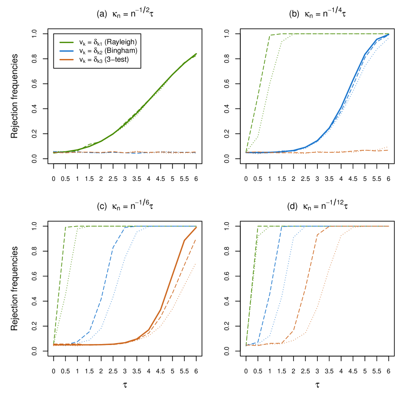
Figure 1: Rejection frequencies of the Rayleigh test (green), of the Bingham test (blue), and of the $3$-test (dark orange), all conducted at asymptotic level $\alpha=5\%$. A collection of $M=2,\!500$ mutually independent random samples of size $n=500$ (dotted lines) and $n=5,\!000$ (dashed lines) were considered from the rotationally symmetric distribution with location $\boldsymbol{\theta}_{0}=(0,0,1)^{\prime}$, angular function $f(s)=\exp(s)$, and concentration $\kappa_{n}=n^{-1/\ell}\tau$, for $\ell=2,4,6,12$ and $\tau\in\{0,0.5,1,\ldots,6\}$. Whenever the rejection frequencies are non-trivial (that is, strictly between $\alpha$ and $1$), the corresponding asymptotic powers are also provided (solid lines).

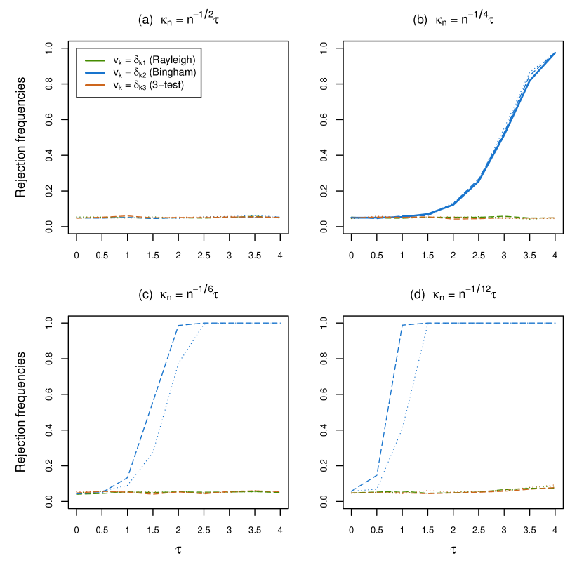
Figure 2: Same results as in Figure 1, but with angular function $f(s)=\exp(s^{2})$ and $\tau\in\{0,0.5,1,\ldots,4\}$.

7 Perspectives for future research

The present paper studied the asymptotic powers of Sobolev tests under local rotationally symmetric alternatives. The results require minimal assumptions (only differentiability assumptions of the angular function $f$ at zero are imposed) and they cover all Sobolev tests. The consistency rate of an arbitrary Sobolev test and the corresponding asymptotic powers were obtained under almost all rotationally symmetric distributions. To be more specific, if the angular function $f$ is infinitely many times differentiable at zero with $f^{\underline{k}}(0)=0$ for any positive integer $k$ (consider for instance the function $f$ such that $f(s)=1+\exp(-1/s^{2})$ for $s\neq 0$ and $f(0)=1$), then our results only state that all Sobolev tests will be blind to local alternatives in $\kappa_{n}\sim n^{-1/(2q)}$ irrespective of the positive integer $q$. As a corollary, consistency rates in this particular case remain unknown (consistency follows from Theorem 4.4 in Giné,, 1975). The consistency rate and resulting local powers could be explored in future work, even though this may be of academic interest only (one may argue that if a test does not show polynomial consistency rates in a specific parametric model, then this test is in any case of low practical relevance in that model).

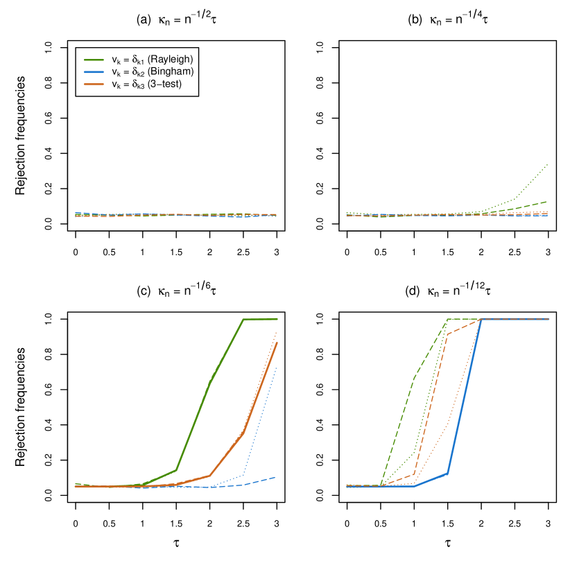
Figure 3: Same results as in Figure 1, but with angular function $f(s)=\exp(s^{3})$ and $\tau\in\{0,0.5,1,\ldots,3\}$.

Another avenue for future research is to consider other distributional setups. Rotationally symmetric distributions involve a single particular direction, namely the direction of $\boldsymbol{\theta}$, hence are “single-spiked” distributions. More general distributions in directional statistics are rather “multi-spiked” ones. For instance, the Bingham, (1974) distributions are multi-spiked extensions of the rotationally symmetric distributions associated with $f(s)=\exp(s^{2})$, that is, extensions of the Watson distributions. It would be of interest to extend the results of the present work by characterizing the local non-null behavior of Sobolev tests against such multi-spiked alternatives. This is by no means easy since, in principle, each “spike” may involve its own concentration parameter $\kappa$. Another possible direction for future research is to go away from the fixed-$p$ setup considered in this paper to consider high-dimensional asymptotic scenarios under which the dimension $p=p_{n}$ diverges to infinity as $n$ does. Consistency rates and local powers in this case are available for very specific Sobolev tests only; we refer to Cutting et al., (2017, 2021), for the Rayleigh test and for the Bingham test, respectively. Results that would apply to arbitrary Sobolev tests in high dimensions would be of interest. This will be considered in future work.

Appendix A Proofs of Section 3

The proof of Proposition 2 requires the following result, that is classical in spherical harmonic analysis; see, e.g., Theorem 1.2.9 in Dai and Xu, (2013).

Theorem 1 (Funk–Hecke Theorem).

Let $p\geq 3$ be an integer and $k$ be a nonnegative integer. Let $h:[-1,1]\to\mathbb{R}$ be a measurable function such that $\int_{-1}^{1}(1-s^{2})^{(p-3)/2}|h(s)|\,\mathrm{d}s$ is finite. Then, for any $\varphi_{k}\in\mathcal{H}^{p}_{k}$ and any $\boldsymbol{\eta}\in\mathcal{S}^{p-1}$,

$$\int_{\mathcal{S}^{p-1}}h(\boldsymbol{\xi}^{\prime}\boldsymbol{\eta})\varphi_{k}(\boldsymbol{\xi})\,\mathrm{d}\sigma_{p}(\boldsymbol{\xi})=\lambda_{k}\varphi_{k}(\boldsymbol{\eta}),$$

with

$$\lambda_{k}=\frac{\omega_{p-2}}{C_{k}^{(p-2)/2}(1)}\int_{-1}^{1}(1-s^{2})^{(p-3)/2}h(s)C_{k}^{(p-2)/2}(s)\,\mathrm{d}s,$$

where $\omega_{p-2}$ is the surface area of $\mathcal{S}^{p-2}$.

Proof of Proposition 2. Throughout, we write $\mathbf{U}:=\mathbf{U}_{1}$. Let us first prove (19) for $p=2$, where $\mathbf{U}=(U_{1},U_{2})^{\prime}$. We have

$${\rm E}^{(n)}_{\kappa_{n},f}[g_{1,k}(\mathbf{U})] =\sqrt{2}{\rm E}^{(n)}_{\kappa_{n},f}[\cos(k\arccos U_{2})\mathbb{I}[U_{1}\geq 0]+\cos(k(2\pi-\arccos U_{2}))\mathbb{I}[U_{1}<0]]$$

$$=\sqrt{2}{\rm E}^{(n)}_{\kappa_{n},f}[\cos(k\arccos U_{2})]=\sqrt{2}{\rm E}^{(n)}_{\kappa_{n},f}[C_{k}^{0}(U_{2})]=\sqrt{2}{\rm E}^{(n)}_{\kappa_{n},f}[C_{k}^{0}(\mathbf{U}^{\prime}\boldsymbol{\theta}_{0})].$$

Similarly, since $U_{1}\neq 0$ almost surely under ${\rm P}^{(n)}_{\kappa_{n},f}$,

$${\rm E}^{(n)}_{\kappa_{n},f}[g_{2,k}(\mathbf{U})] =\sqrt{2}{\rm E}^{(n)}_{\kappa_{n},f}[\sin(k\arccos U_{2})\mathbb{I}[U_{1}>0]+\sin(k(2\pi-\arccos U_{2}))\mathbb{I}[U_{1}<0]]$$

$$=\sqrt{2}{\rm E}^{(n)}_{\kappa_{n},f}[\sin(k\arccos U_{2})(\mathbb{I}[U_{1}>0]-\mathbb{I}[U_{1}<0])]=0,$$

where the last equality results from the fact, the distribution being rotationally symmetric about $\boldsymbol{\theta}_{0}=(0,1)^{\prime}$, we have that $(-U_{1},U_{2})$ and $(U_{1},U_{2})$ are equal in distribution under ${\rm P}^{(n)}_{\kappa_{n},f}$. This establishes (19) for $p=2$. For $p\geq 3$, taking $h(s)=c_{p,\kappa_{n},f}f(\kappa_{n}s)$ in Theorem 1 yields, for $r=1,\ldots,d_{p,k}$,

$$\mathrm{E}^{(n)}_{\kappa_{n},f}[{g}_{r,k}(\mathbf{U})] =\frac{1}{\omega_{p-2}}\int_{\mathcal{S}^{p-1}}h(\mathbf{x}^{\prime}\boldsymbol{\theta}_{0}){g}_{r,k}(\mathbf{x})\,\mathrm{d}\sigma_{p}(\mathbf{x})=\frac{\lambda_{k}{g}_{r,k}(\boldsymbol{\theta}_{0})}{\omega_{p-2}}$$

$$=\frac{1}{C_{k}^{(p-2)/2}(1)}\bigg{(}c_{p,\kappa_{n},f}\int_{-1}^{1}(1-s^{2})^{(p-3)/2}f(\kappa_{n}s)C_{k}^{(p-2)/2}(s)\,\mathrm{d}s\bigg{)}{g}_{r,k}(\boldsymbol{\theta}_{0})$$

$$=\frac{1}{C_{k}^{(p-2)/2}(1)}\mathrm{E}^{(n)}_{\kappa_{n},f}[C_{k}^{(p-2)/2}(\mathbf{U}^{\prime}\boldsymbol{\theta}_{0})]{g}_{r,k}(\boldsymbol{\theta}_{0}).$$

Recalling that $\boldsymbol{\theta}_{0}=(0,\ldots,0,1)^{\prime}\in\mathbb{R}^{p}$, (19) then follows from the fact that

$$g_{1,k}(\boldsymbol{\theta}_{0}) =\frac{1}{\sqrt{d_{p,k}}}\Big{(}1+\frac{2k}{p-2}\Big{)}C_{k}^{(p-2)/2}(1),$$

$$g_{r,k}(\boldsymbol{\theta}_{0}) =0,\quad r=2,\ldots,d_{p,k};$$

see (11)–(12).

In view of (16)–(17), it remains to show that, as $n\to\infty$,

$${\rm E}_{\kappa_{n},f}^{(n)}[g_{r,k}(\mathbf{U})g_{s,\ell}(\mathbf{U})]={\rm E}_{0}^{(n)}[g_{r,k}(\mathbf{U})g_{s,\ell}(\mathbf{U})]+o(1)$$ (27)

for any $k,\ell\in\{0,1,\ldots,\}$, $r\in\{1,\ldots,d_{p,k}\}$, and $s\in\{1,\ldots,d_{p,\ell}\}$ (recall that $d_{p,0}=1$ and $g_{1,0}\equiv 1$). To do so, note that the continuity of $f$ at zero implies that

$$\sup_{\mathbf{u}\in\mathcal{S}^{p-1}}|f(\kappa_{n}\mathbf{u}^{\prime}\boldsymbol{\theta})-f(0)|=\sup_{s\in[-1,1]}|f(\kappa_{n}s)-f(0)|\to 0,$$

hence that

$$|c_{p,\kappa_{n},f}^{-1}-c_{p}^{-1}| \leq\int_{-1}^{1}|f(\kappa_{n}s)-f(0)|(1-s^{2})^{(p-3)/2}\,\mathrm{d}s$$

$$\leq\sup_{s\in[-1,1]}|f(\kappa_{n}s)-f(0)|\int_{-1}^{1}(1-s^{2})^{(p-3)/2}\,\mathrm{d}s\to 0$$

as $n$ diverges to infinity. Therefore,

$$\sup_{\mathbf{u}\in\mathcal{S}^{p-1}}|c_{p,\kappa_{n},f}f(\kappa_{n}\mathbf{u}^{\prime}\boldsymbol{\theta})-c_{p}f(0)|\to 0$$

as $n$ diverges to infinity. It then follows that

$$\bigg{|}\int_{\mathcal{S}^{p-1}} g_{r,k}(\mathbf{u})g_{s,\ell}(\mathbf{u})(c_{p,\kappa_{n},f}f(\kappa_{n}\mathbf{u}^{\prime}\boldsymbol{\theta})-c_{p}f(0))\,\mathrm{d}\sigma_{p}(\mathbf{u})\bigg{|}$$

$$\leq\sup_{\mathbf{u}\in\mathcal{S}^{p-1}}|c_{p,\kappa_{n},f}f(\kappa_{n}\mathbf{u}^{\prime}\boldsymbol{\theta})-c_{p}f(0)|\int_{\mathcal{S}^{p-1}}|g_{r,k}(\mathbf{u})g_{s,\ell}(\mathbf{u})|\,\mathrm{d}\sigma_{p}(\mathbf{u})\to 0$$

as $n$ diverges to infinity, which establishes (27), hence proves the result. ∎

The proof of Proposition 3 requires the following preliminary result.

Lemma 1.

Fix integers $p\geq 2$, $k>0$, and $m\geq 0$. Let $g:\mathbb{R}\to\mathbb{R}$ be $k$ times differentiable at zero and let $(\kappa_{n})$ be a positive real sequence that is $o(1)$. Then, as $n$ diverges to infinity,

$$R_{n}^{(m)}(g):=c_{p}\int_{-1}^{1}(1-s^{2})^{(p-3)/2}s^{m}g(\kappa_{n}s)\,\mathrm{d}s=\sum_{\ell=0}^{k}\frac{a_{m+\ell}}{\ell!}\kappa_{n}^{\ell}g^{\underline{\ell}}(0)+o({\kappa_{n}^{k}}).$$

Proof of Lemma 1. First note that (22) yields

$$R_{n}^{(m)}(g)-\sum_{\ell=0}^{k-1}\frac{a_{m+\ell}}{\ell!}\kappa_{n}^{\ell}g^{\underline{\ell}}(0)=c_{p}\int_{-1}^{1}(1-s^{2})^{(p-3)/2}s^{m}\bigg{\{}g(\kappa_{n}s)-\sum_{\ell=0}^{k-1}\frac{(\kappa_{n}s)^{\ell}}{\ell!}g^{\underline{\ell}}(0)\bigg{\}}\,\mathrm{d}s.$$

Letting $t=\kappa_{n}s$ and using (22) again then provides

$$R_{n}^{(m)}(g)-\sum_{\ell=0}^{k-1}\frac{a_{m+\ell}}{\ell!}\kappa_{n}^{\ell}g^{\underline{\ell}}(0)={a_{m+k}\kappa_{n}^{k}}\int_{-\infty}^{\infty}h_{n}(t)\bigg{(}\frac{g(t)-\sum_{\ell=0}^{k-1}\frac{t^{\ell}}{\ell!}g^{\underline{\ell}}(0)}{t^{k}}\bigg{)}\,\mathrm{d}t,$$

where $h_{n}$ is defined through

$$t\mapsto h_{n}(t)=\frac{(\textstyle\frac{t}{\kappa_{n}})^{m+k}(1-(\textstyle\frac{t}{\kappa_{n}})^{2})^{(p-3)/2}}{\int_{-\kappa_{n}}^{\kappa_{n}}(\textstyle\frac{s}{\kappa_{n}})^{m+k}(1-(\textstyle\frac{s}{\kappa_{n}})^{2})^{(p-3)/2}\,\mathrm{d}s}\,\mathbb{I}[|t|\leq\kappa_{n}].$$

It can be checked that, since $\kappa_{n}=o(1)$, the $h_{n}$’s form an approximate $\delta$-sequence, in the sense that $\int_{-\infty}^{\infty}h_{n}(t)\,\mathrm{d}t=1$ for all $n$ and $\int_{-\varepsilon}^{\varepsilon}h_{n}(t)\,\mathrm{d}t\to 1$ for any $\varepsilon>0$. Hence,

$$R_{n}^{(m)}(g)-\sum_{\ell=0}^{k-1}\frac{a_{m+\ell}}{\ell!}\kappa_{n}^{\ell}g^{\underline{\ell}}(0)={a_{m+k}\kappa_{n}^{k}}\,\lim_{t\to 0}\bigg{(}\frac{g(t)-\sum_{\ell=0}^{k-1}\frac{t^{\ell}}{\ell!}g^{\underline{\ell}}(0)}{t^{k}}\bigg{)}+o\big{(}{\kappa_{n}^{k}}\big{)}$$

which yields the result by first using L’Hôpital’s rule $k-1$ times and then the differentiability of $g^{\underline{k-1}}$ at zero. ∎

The following result is a direct corollary of Lemma 1 with $m=0$.

Lemma 2.

Fix integers $p\geq 2$ and $k>0$. Let $(\kappa_{n})$ be a positive real sequence that is $o(1)$ and $f$ be an angular function that is $k$ times differentiable at zero. Then, as $n$ diverges to infinity,

$$\frac{c_{p,\kappa_{n},f}}{c_{p}}=\Bigg{(}\sum_{\ell=0}^{k}\frac{a_{\ell}}{\ell!}\kappa_{n}^{\ell}f^{\underline{\ell}}(0)+o({\kappa_{n}^{k}})\Bigg{)}^{-1},$$

where $c_{p,\kappa,f}$ is the normalizing constant in (5).

We can now prove Proposition 3.

Proof of Proposition 3. Writing

$$e_{n,m}=\bigg{(}\frac{c_{p,\kappa_{n},f}}{c_{p}}\bigg{)}c_{p}\int_{-1}^{1}(1-s^{2})^{(p-3)/2}s^{m}f(\kappa_{n}s)\,\mathrm{d}s$$

and using Lemmas 1–2 with $k=q-m$ provides

$$e_{n,m} =\Bigg{(}\sum_{\ell=0}^{q-m}\frac{a_{\ell}}{\ell!}\kappa_{n}^{\ell}f^{\underline{\ell}}(0)+o({\kappa_{n}^{q-m}})\Bigg{)}^{-1}\Bigg{(}\sum_{\ell=0}^{q-m}\frac{a_{m+\ell}}{\ell!}\kappa_{n}^{\ell}f^{\underline{\ell}}(0)+o({\kappa_{n}^{q-m}})\Bigg{)}$$

$$=\Bigg{(}\sum_{\ell=0}^{q-m}\beta_{\ell}\kappa_{n}^{\ell}+o({\kappa_{n}^{q-m}})\Bigg{)}^{-1}\Bigg{(}\sum_{\ell=0}^{q-m}\alpha_{\ell}\kappa_{n}^{\ell}+o({\kappa_{n}^{q-m}})\Bigg{)},$$

where we let

$$\beta_{\ell}:=\frac{a_{\ell}}{\ell!}f^{\underline{\ell}}(0)\quad\textrm{ and }\quad\alpha_{\ell}:=\frac{a_{\ell+m}}{\ell!}f^{\underline{\ell}}(0).$$

This yields

$$e_{n,m}=\sum_{\ell=0}^{q-m}b_{m,\ell}\kappa_{n}^{\ell}+o({\kappa_{n}^{q-m}}),$$

where the coefficients $b_{m,\ell}$ satisfy

$$\sum_{j=0}^{\ell}\beta_{\ell-j}b_{m,j}=\alpha_{\ell},\quad\ell=0,1,\ldots,q-m,$$

or equivalently, where ${\bf b}_{m}=(b_{m,0},b_{m,1},\ldots,b_{m,q-m})^{\prime}$ satisfies $\mathbf{A}_{q-m}{\bf b}_{m}=\mathbf{v}_{q-m}^{(m)}$. ∎

The proof of Proposition 4 requires the following lemma.

Lemma 3.

For any positive integers $j,k$ and for any integer $p\geq 2$,

$$c_{p}\int_{-1}^{1}C_{k}^{(p-2)/2}(s)C_{j}^{(p-2)/2}(s)(1-s^{2})^{(p-3)/2}\,\mathrm{d}s=\frac{\delta_{kj}}{t_{p,k}^{2}},$$

where $t_{p,k}$ was defined in Proposition 2.

Proof of Lemma 3. For $p=2$, the result follows from the fact that $c_{2}=1/\pi$ (see (6)) and the identity

$$\int_{-1}^{1}C_{k}^{0}(s)C_{j}^{0}(s)(1-s^{2})^{-1/2}\,\mathrm{d}s=\frac{\pi}{2}\delta_{jk};$$

see, e.g., Equation 3.11.8 in DLMF, (2020). For $p=3$, Corollary 1.2.8 in Dai and Xu, (2013) entails that

$$c_{p}\int_{-1}^{1}C_{k}^{(p-2)/2}(s) C_{j}^{(p-2)/2}(s)(1-s^{2})^{(p-3)/2}\,\mathrm{d}s$$

$$=\frac{c_{p}\omega_{p-1}}{\omega_{p-2}}\Big{(}1+\frac{2k}{p-2}\Big{)}^{-1}C_{k}^{(p-2)/2}(1)\delta_{jk}.$$ (28)

Using

$$g_{1,k}(\boldsymbol{\theta}_{0}) =\frac{1}{\sqrt{d_{p,k}}}\Big{(}1+\frac{2k}{p-2}\Big{)}C_{k}^{(p-2)/2}(1),$$

$$g_{r,k}(\boldsymbol{\theta}_{0}) =0,\quad r=2,\ldots,d_{p,k}$$

in the addition formula (13) with $\mathbf{u}=\mathbf{v}=\boldsymbol{\theta}_{0}$, we obtain the identity

$$C_{k}^{(p-2)/2}(1)=\Big{(}1+\frac{2k}{p-2}\Big{)}^{-1}d_{p,k}.$$ (29)

Plugging this and the identity $c_{p}\omega_{p-1}=\omega_{p-2}$ (which follows from (6)) into (28) then yields the result. ∎

We can now prove Proposition 4.

Proof of Proposition 4. Using (8), Proposition 3 (with $q=2(k-j)+r>k-2j=m$) yields

$${\rm E}^{(n)}_{\kappa_{n},f}[C_{k}^{(p-2)/2}(\mathbf{U}_{1}^{\prime}\boldsymbol{\theta}_{0})] =\sum_{j=0}^{\lfloor k/2\rfloor}(-1)^{j}c^{(p-2)/2}_{k,j}e_{n,k-2j}$$

$$=\sum_{j=0}^{\lfloor k/2\rfloor}(-1)^{j}c^{(p-2)/2}_{k,j}\bigg{(}\sum_{\ell=0}^{k+r}b_{k-2j,\ell}\kappa_{n}^{\ell}+o\big{(}{\kappa_{n}^{k+r}}\big{)}\bigg{)}$$

$$=\sum_{\ell=0}^{k+r}w_{\ell}\kappa_{n}^{\ell}+o({\kappa_{n}^{k+r}}),$$ (30)

with

$$w_{\ell}:=\sum_{j=0}^{\lfloor k/2\rfloor}(-1)^{j}c^{(p-2)/2}_{k,j}b_{k-2j,\ell}.$$

Letting $\mathbf{w}:=(w_{0},w_{1},\ldots,w_{k+r})^{\prime}$, we have

$$\mathbf{w} =\sum_{j=0}^{\lfloor k/2\rfloor}(-1)^{j}c^{(p-2)/2}_{k,j}(b_{k-2j,0},b_{k-2j,1},\ldots,b_{k-2j,k+r})^{\prime}$$

$$=\mathbf{A}_{k+r}^{-1}\Bigg{(}\sum_{j=0}^{\lfloor k/2\rfloor}(-1)^{j}c^{(p-2)/2}_{k,j}\mathbf{v}_{k+r}^{(k-2j)}\Bigg{)},$$ (31)

where $\mathbf{A}_{k+r}$ and $\mathbf{v}_{k+r}^{(k-2j)}$ are as in Proposition 3. Now, for $i=0,1,\ldots,k+r$,

$$\Bigg{(}\sum_{j=0}^{\lfloor k/2\rfloor}(-1)^{j}c^{(p-2)/2}_{k,j}\mathbf{v}_{k+r}^{(k-2j)}\Bigg{)}_{i} =\sum_{j=0}^{\lfloor k/2\rfloor}(-1)^{j}c^{(p-2)/2}_{k,j}\bigg{(}a_{k-2j+i}\frac{f^{\underline{i}}(0)}{i!}\bigg{)}$$

$$=\frac{f^{\underline{i}}(0)}{i!}{\rm E}_{0}^{(n)}\Bigg{[}(\mathbf{U}_{1}^{\prime}\boldsymbol{\theta}_{0})^{i}\sum_{j=0}^{\lfloor k/2\rfloor}(-1)^{j}c^{(p-2)/2}_{k,j}(\mathbf{U}_{1}^{\prime}\boldsymbol{\theta}_{0})^{k-2j}\Bigg{]}$$

$$=\frac{f^{\underline{i}}(0)}{i!}{\rm E}_{0}^{(n)}\big{[}(\mathbf{U}_{1}^{\prime}\boldsymbol{\theta}_{0})^{i}C_{k}^{(p-2)/2}(\mathbf{U}_{1}^{\prime}\boldsymbol{\theta}_{0})\big{]}.$$

Recalling (23), this yields

$$\Bigg{(}\sum_{j=0}^{\lfloor k/2\rfloor}(-1)^{j}c^{(p-2)/2}_{k,j}\mathbf{v}_{k+r}^{(k-2j)}\Bigg{)}_{i} =\frac{f^{\underline{i}}(0)}{i!}\sum_{j=0}^{i}m_{j,i}{\rm E}_{0}^{(n)}\big{[}C_{j}^{(p-2)/2}(\mathbf{U}_{1}^{\prime}\boldsymbol{\theta}_{0})C_{k}^{(p-2)/2}(\mathbf{U}_{1}^{\prime}\boldsymbol{\theta}_{0})\big{]}$$

$$=\frac{f^{\underline{i}}(0)}{(i!)t_{p,k}^{2}}m_{k,i}\mathbb{I}[k\leq i]=\frac{1}{t_{p,k}^{2}}\Big{(}{\bf z}_{k+r}^{(k)}\Big{)}_{i},$$

where we applied Lemma 3. Using this in (30)–(31), we obtain that, with the vector ${\bf z}_{q-k}$ defined in the statement of the proposition,

$${\rm E}_{\kappa_{n},f}^{(n)}\big{[}C_{k}^{(p-2)/2}(\mathbf{U}_{1}^{\prime}\boldsymbol{\theta}_{0})\big{]} =\sum_{\ell=0}^{k+r}({\bf e}_{\ell+1,k+r+1}^{\prime}{\bf w})\kappa_{n}^{\ell}+o({\kappa_{n}^{k+r}})$$

$$=\frac{1}{t_{p,k}^{2}}\sum_{\ell=k}^{k+r}({\bf e}_{\ell+1,k+r+1}^{\prime}\mathbf{A}_{k+r}^{-1}{\bf z}_{k+r}^{(k)})\kappa_{n}^{\ell}+o({\kappa_{n}^{k+r}}),$$ (32)

where the terms associated with $\ell=0,1,\ldots,k-1$ cancel since $\mathbf{A}_{k+r}^{-1}$ is a lower triangular matrix and the first $k$ components of ${\bf z}_{k+r}^{(k)}$ are zero. Since ${\bf e}_{\ell+1,k+r+1}^{\prime}\mathbf{A}_{k+r}^{-1}={\bf a}_{\ell+1;k+r}^{\prime}$, the result is proved. ∎

Appendix B Proofs of Section 4

Proof of Proposition 5. For any $i=1,\ldots,n$, consider the random vector $\mathbf{Z}_{i}:=(({\bf G}_{p,1}(\mathbf{U}_{i}))^{\prime},\ldots,\allowbreak({\bf G}_{p,K}(\mathbf{U}_{i}))^{\prime})^{\prime}$, with dimension $d:=d_{p,1}+\cdots+d_{p,K}$. Using the classical Cramér–Wold device, we need to show that, for any $\mathbf{w}\in\mathcal{S}^{d-1}$,

$$\sqrt{n}\mathbf{w}^{\prime}({\bf T}_{p,K}^{(n)}-{\rm E}^{(n)}_{\kappa_{n},f}[{\bf T}_{p,K}^{(n)}])=\frac{1}{\sqrt{n}}\sum_{i=1}^{n}(\mathbf{w}^{\prime}\mathbf{Z}_{i}-{\rm E}^{(n)}_{\kappa_{n},f}[\mathbf{w}^{\prime}\mathbf{Z}_{i}])=:\sum_{i=1}^{n}X_{ni}$$

is asymptotically standard normal. From Proposition 2, we have that

$$s_{n}^{2}:= \;{\rm Var}^{(n)}_{\kappa_{n},f}\Bigg{[}\sum_{i=1}^{n}X_{ni}\Bigg{]}=n{\rm Var}^{(n)}_{\kappa_{n},f}[X_{n1}]=\mathbf{w}^{\prime}{\rm Var}^{(n)}_{\kappa_{n},f}[\mathbf{Z}_{1}]\mathbf{w}$$

$$= \;\mathbf{w}^{\prime}{\rm diag}({\bf I}_{d_{p,1}},\ldots,{\bf I}_{d_{p,K}})\mathbf{w}+o(1)=1+o(1)$$

as $n$ diverges to infinity. Now, since each component $g_{r,k}$ of ${\bf G}_{p,k}$, $k=1,\ldots,K$, is a continuous function defined over the compact set $\mathcal{S}^{p-1}$, there exists a positive constant $C$ such that

$$\max_{k=1,\ldots,K}\max_{r=1,\ldots,d_{p,k}}\sup_{u\in\mathcal{S}^{p-1}}|g_{r,k}(\mathbf{u})|\leq C,$$

which implies that

$$|X_{ni}|\leq\frac{1}{\sqrt{n}}\|\mathbf{Z}_{i}-{\rm E}^{(n)}_{\kappa_{n},f}[\mathbf{Z}_{i}]\|\leq\frac{1}{\sqrt{n}}(\|\mathbf{Z}_{i}\|+\|{\rm E}^{(n)}_{\kappa_{n},f}[\mathbf{Z}_{i}]\|)\leq\frac{2\sqrt{d}C}{\sqrt{n}}$$

almost surely. Therefore,

$$\frac{1}{s_{n}^{3}}\sum_{i=1}^{n}{\rm E}[|X_{ni}|^{3}]\leq\frac{8d^{3/2}C^{3}}{s_{n}^{3}\sqrt{n}}\to 0$$

as $n$ diverges to infinity. The result thus follows from the Liapounov central limit theorem; see, e.g., Theorem 5.2 in DasGupta, (2008). ∎

Proof of Theorem 2. By definition of $k_{v}$ and $K_{v}$,

$$S^{(n)}_{v}=n({\bf T}_{p,k_{v},K_{v}}^{(n)})^{\prime}{\rm diag}(v_{k_{v}}^{2}{\bf I}_{d_{p,k_{v}}},\ldots,v_{K_{v}}^{2}{\bf I}_{d_{p,K_{v}}}){\bf T}_{p,k_{v},K_{v}}^{(n)},$$

with

$${\bf T}_{p,k,K}^{(n)}:=\frac{1}{n}\sum_{i=1}^{n}(({\bf G}_{p,k}(\mathbf{U}_{i}))^{\prime},\ldots,({\bf G}_{p,K}(\mathbf{U}_{i}))^{\prime})^{\prime}.$$

Decompose then $\sqrt{n}{\bf T}_{p,k,K}^{(n)}$ into

$$\sqrt{n}{\bf T}_{p,k_{v},K_{v}}^{(n)} =\sqrt{n}\big{(}{\bf T}_{p,k_{v},K_{v}}^{(n)}-{\rm E}^{(n)}_{\kappa_{n},f}[{\bf T}_{p,k_{v},K_{v}}^{(n)}]\big{)}+\sqrt{n}{\rm E}^{(n)}_{\kappa_{n},f}[{\bf T}_{p,k_{v},K_{v}}^{(n)}]$$

$$=:V_{n}+W_{n},$$

say. Now, it directly follows from Proposition 5 that $V_{n}$ is asymptotically standard normal. For $W_{n}$, we need to consider cases (i)–(iii) separately. In case (i), Propositions 2 and 4 entail that $W_{n}=o(1)$ as $n\rightarrow\infty$, which establishes the result. In case (ii), under which $\kappa_{n}=n^{-1/(2k_{v})}\tau$, Propositions 2 and 4 provide

$$W_{n}=\frac{m_{k_{v},k_{v}}f^{\underline{k_{v}}}(0)}{(k_{v}!)t_{p,k_{v}}}\tau^{k_{v}}{{\bf e}_{1,d_{p,k_{v}}}\choose{\bf 0}}+o(1)$$ (33)

as $n\rightarrow\infty$. The result then follows from the fact that, for any positive integer $k$,

$$m_{k,k}=\frac{1}{c^{0}_{k,0}}=\frac{1}{2^{k-1}}$$

for $p=2$, and

$$m_{k,k}=\frac{1}{c^{(p-2)/2}_{k,0}}=\frac{2^{-k}k!\Gamma(\frac{p-2}{2})}{\Gamma(\frac{p-2}{2}+k)}=\frac{k!}{2^{k}(\frac{p-2}{2})_{k}}$$

for $p\geq 3$; see (8), (9), and (23). Finally, in case (iii), Propositions 2 and 4 now entail

$$W_{n}=r_{n}{{\bf e}_{1,d_{p,k_{v}}}\choose{\bf 0}},$$ (34)

where $|r_{n}|\to\infty$ as $n\rightarrow\infty$. This establishes the result. ∎

Proof of Theorem 3. (i) For any $k\in\{k_{v},k_{v}+1,\ldots,K_{v}\}$, applying Proposition 2, then Proposition 4 with $r=q-k$, yields

$$\mathrm{E}^{(n)}_{\kappa_{n},f}[{\bf G}_{p,k}(\mathbf{U}_{1})] =\frac{1}{t_{p,k}}\sum_{\ell=k}^{q}({\bf a}_{\ell+1;q}^{\prime}{\bf z}^{(k)}_{q})\kappa_{n}^{\ell}{\bf e}_{1}+o(\kappa_{n}^{q})$$

$$=\frac{1}{t_{p,k}}\sum_{\ell=k}^{q}\;\sum_{i=k}^{\ell}\frac{1}{i!}(\mathbf{A}_{q}^{-1})_{\ell+1,i+1}m_{k,i}f^{\underline{i}}(0)\kappa_{n}^{\ell}{\bf e}_{1}+o(\kappa_{n}^{q}),$$ (35)

where the sum over $i$ stops at $\ell$ due to the lower triangular nature of $\mathbf{A}_{q}^{-1}$. As noted below Proposition 4, ${\bf A}_{q}^{-1}=\sum_{j=0}^{q}(-1)^{j}\mathbf{L}_{q}^{j}$, where $\mathbf{L}_{q}$ is a strictly lower triangular matrix. Since $(\mathbf{L}_{q})_{rs}$ is zero if $r-s$ is odd, it follows that a necessary condition for $(\mathbf{A}_{q}^{-1})_{\ell+1,i+1}\neq 0$ is that $\ell\sim i$. Recalling that, similarly, a necessary condition for $m_{k,i}\neq 0$ is that $k\sim i$, (35) rewrites

$$\mathrm{E}^{(n)}_{\kappa_{n},f}[{\bf G}_{p,k}(\mathbf{U}_{1})]=\frac{1}{t_{p,k}}\sum_{\begin{subarray}{c}k\leq\ell\leq q\\ \ell\sim k\end{subarray}}s_{k,\ell}\kappa_{n}^{\ell}{\bf e}_{1}+o(\kappa_{n}^{q}),$$ (36)

with

$$s_{k,\ell}=s_{k,\ell,q}:=\sum_{\begin{subarray}{c}k\leq i\leq\ell\\ i\sim k\end{subarray}}\frac{1}{i!}(\mathbf{A}_{q}^{-1})_{\ell+1,i+1}m_{k,i}f^{\underline{i}}(0).$$

We then consider three cases. (A) Fix $k\in\{k_{v},\ldots,k_{\dagger}-1\}\,\cap\,{\rm Supp}(v)$, where ${\rm Supp}(v):=\{k:v_{k}\neq 0\}$. Then, there cannot exist $i\in\{k,k+1,\ldots,k_{*}\}$ such that $i\sim k$ and $f^{\underline{i}}(0)\neq 0$ (the existence of such an integer $i$ would indeed contradict the definition of $k_{*}$ for $i<k_{*}$ and the definition of $k_{\dagger}$ for $i=k_{*}$). It follows that

$$\mathrm{E}^{(n)}_{\kappa_{n},f}[{\bf G}_{p,k}(\mathbf{U}_{1})]=O(\kappa_{n}^{k_{*}+1}),$$

so that $\sqrt{n}\mathrm{E}^{(n)}_{\kappa_{n},f}[{\bf G}_{p,k}(\mathbf{U}_{1})]=o(1)$. (B) Fix $k\in\{k_{\dagger},k_{\dagger}+1,\ldots,k_{*}\}\cap{\rm Supp}(v)$. The same argument as in Case (A) implies that there is no $i\in\{k,k+1,\ldots,k_{*}-1\}$ such that $i\sim k$ and $f^{\underline{i}}(0)\neq 0$. Therefore,

$$\mathrm{E}^{(n)}_{\kappa_{n},f}[{\bf G}_{p,k}(\mathbf{U}_{1})]=\frac{1}{t_{p,k}}s_{k,k_{*}}\kappa_{n}^{k_{*}}\mathbb{I}[k\sim k_{*}]{\bf e}_{1}+o(\kappa_{n}^{k_{*}}),$$

where $s_{k,k_{*}}=(k_{*}!)^{-1}m_{k,k_{*}}f^{\underline{k_{*}}}(0)$ (recall that the diagonal entries of $\mathbf{A}_{q}^{-1}$ are equal to one), which yields

$$\sqrt{n}\mathrm{E}^{(n)}_{\kappa_{n},f}[{\bf G}_{p,k}(\mathbf{U}_{1})]=\frac{m_{k,k_{*}}f^{\underline{k_{*}}}(0)\tau^{k_{*}}}{(k_{*}!)t_{p,k}}\mathbb{I}[k\sim k_{*}]{\bf e}_{1}+o(1).$$

(C) Fix $k\in\{k_{*}+1,\ldots,K_{v}\}\,\cap\,{\rm Supp}(v)$. Then, (36) trivially implies that $\mathrm{E}^{(n)}_{\kappa_{n},f}[{\bf G}_{p,k}(\mathbf{U}_{1})]=o(\kappa_{n}^{k_{*}})$, so that

$$\sqrt{n}\mathrm{E}^{(n)}_{\kappa_{n},f}[{\bf G}_{p,k}(\mathbf{U}_{1})]=o(1).$$

Summing up, for any $k\in{\rm Supp}(v)$,

$$\sqrt{n}\mathrm{E}^{(n)}_{\kappa_{n},f}[{\bf G}_{p,k}(\mathbf{U}_{1})]=\frac{m_{k,k_{*}}f^{\underline{k_{*}}}(0)\tau^{k_{*}}}{(k_{*}!)t_{p,k}}\mathbb{I}[k\sim k_{*},k_{\dagger}\leq k\leq k_{*}]{\bf e}_{1}+o(1).$$

The weak limit result in Part (i) of the theorem then follows as in the proof of Theorem 2(ii). Since Part (ii) follows in the exact same way, it only remains to show that $\xi_{p,k,k_{*}}(\tau)$ admits the alternative expression provided in the statement of the theorem. Clearly, it is sufficient to show that

$$\frac{m_{k,k_{*}}}{t_{p,k}^{2}}=\sum_{j=0}^{\lfloor k/2\rfloor}(-1)^{j}c^{(p-2)/2}_{k,j}a_{k+k_{*}-2j}.$$ (37)

To do so, note that, for any integer $k_{*}>0$ and any $k\in\{1,\ldots,k_{*}\}$, Lemma 3 yields

$$c_{p}\int_{-1}^{1} C_{k}^{(p-2)/2}(s)s^{k_{*}}(1-s^{2})^{(p-3)/2}\,\mathrm{d}s$$

$$=c_{p}\sum_{\ell=0}^{k_{*}}m_{\ell,k_{*}}\int_{-1}^{1}C_{k}^{(p-2)/2}(s)C_{\ell}^{(p-2)/2}(s)(1-s^{2})^{(p-3)/2}\,\mathrm{d}s$$

$$=\sum_{\ell=0}^{k_{*}}\frac{m_{\ell,k_{*}}\delta_{k\ell}}{t_{p,k}^{2}}=\frac{m_{k,k_{*}}}{t_{p,k}^{2}}\cdot$$

Now, using (8) and (9) (for $p\geq 3$ and $p=2$, respectively), then (22), we also have

$$c_{p}\int_{-1}^{1} C_{k}^{(p-2)/2}(s)s^{k_{*}}(1-s^{2})^{(p-3)/2}\,\mathrm{d}s$$

$$=\sum_{j=0}^{\lfloor k/2\rfloor}(-1)^{j}c^{(p-2)/2}_{k,j}\bigg{(}c_{p}\int_{-1}^{1}s^{k-2j}s^{k_{*}}(1-s^{2})^{(p-3)/2}\,\mathrm{d}s\bigg{)}$$

$$=\sum_{j=0}^{\lfloor k/2\rfloor}(-1)^{j}c^{(p-2)/2}_{k,j}a_{k+k_{*}-2j},$$

which establishes (37), hence the theorem. ∎

Appendix C Proofs of Section 5

Proof of Theorem 4. We start with the proof of Part (ii) of the result. For any integer $K\geq k_{v}$, consider the truncated Sobolev test statistic

$$S^{(n)}_{v,K}:=\sum_{k=k_{v}}^{K}v_{k}^{2}\bigg{\|}\frac{1}{\sqrt{n}}\sum_{i=1}^{n}{\bf G}_{p,k}(\mathbf{U}_{i})\bigg{\|}^{2};$$

see (14) and (26). We first show that there exists a positive integer $N$ such that the Sobolev statistic $S^{(n)}_{v}$ in (26) satisfies

$$\sup_{n\geq N}{\rm E}^{(n)}_{\kappa_{n},f}[|S^{(n)}_{v}-S^{(n)}_{v,K}|]=o(1)$$ (38)

as $K$ diverges to infinity. To do so, first note that

$${\rm E}^{(n)}_{\kappa_{n},f}[|S^{(n)}_{v}-S^{(n)}_{v,K}|] ={\rm E}^{(n)}_{\kappa_{n},f}\Bigg{[}\sum_{k=K+1}^{\infty}v_{k}^{2}\bigg{\|}\frac{1}{\sqrt{n}}\sum_{i=1}^{n}{\bf G}_{p,k}(\mathbf{U}_{i})\bigg{\|}^{2}\Bigg{]}$$

$$=\sum_{k=K+1}^{\infty}v_{k}^{2}{\rm E}^{(n)}_{\kappa_{n},f}\Bigg{[}\frac{1}{n}\sum_{i,j=1}^{n}({\bf G}_{p,k}(\mathbf{U}_{i}))^{\prime}{\bf G}_{p,k}(\mathbf{U}_{j})\Bigg{]},$$

where we used the monotone convergence theorem. Hence,

$${\rm E}^{(n)}_{\kappa_{n},f} [|S^{(n)}_{v}-S^{(n)}_{v,K}|]$$

$$=\sum_{k=K+1}^{\infty}v_{k}^{2}\big{\{}{\rm E}^{(n)}_{\kappa_{n},f}[\|{\bf G}_{p,k}(\mathbf{U}_{1})\|^{2}]+(n-1)({\rm E}^{(n)}_{\kappa_{n},f}[{\bf G}_{p,k}(\mathbf{U}_{1})])^{\prime}{\rm E}^{(n)}_{\kappa_{n},f}[{\bf G}_{p,k}(\mathbf{U}_{2})]\big{\}}$$

$$=\sum_{k=K+1}^{\infty}v_{k}^{2}\big{\{}d_{p,k}+(n-1)t_{p,k}^{2}\,\big{(}\mathrm{E}_{\kappa_{n},f}^{(n)}[C_{k}^{(p-2)/2}(\mathbf{U}_{1}^{\prime}\boldsymbol{\theta}_{0})]\big{)}^{2}\big{\}},$$

where the last equality follows from (13), (29), and Proposition 2. Now, for $k\geq k_{v}$, one has

$$\mathrm{E}_{\kappa_{n},f}^{(n)} [C_{k}^{(p-2)/2}(\mathbf{U}_{1}^{\prime}\boldsymbol{\theta}_{0})]$$

$$=\mathrm{E}_{\kappa_{n},f}^{(n)}[C_{k}^{(p-2)/2}(\mathbf{U}_{1}^{\prime}\boldsymbol{\theta}_{0})]-\frac{c_{p,\kappa_{n},f}}{c_{p}}\sum_{\ell=0}^{k_{v}-1}\frac{f^{\underline{\ell}}(0)}{\ell!}\kappa_{n}^{\ell}\mathrm{E}_{0}^{(n)}[(\mathbf{U}_{1}^{\prime}\boldsymbol{\theta}_{0})^{\ell}C_{k}^{(p-2)/2}(\mathbf{U}_{1}^{\prime}\boldsymbol{\theta}_{0})]$$

$$=c_{p,\kappa_{n},f}\int_{-1}^{1}C_{k}^{(p-2)/2}(s)(1-s^{2})^{(p-3)/2}\bigg{\{}f(\kappa_{n}s)-\sum_{\ell=0}^{k_{v}-1}\frac{f^{\underline{\ell}}(0)}{\ell!}\kappa_{n}^{\ell}s^{\ell}\bigg{\}}\,\mathrm{d}s,$$

which, by using the Cauchy–Schwartz inequality, yields

$$\big{(}\mathrm{E}_{\kappa_{n},f}^{(n)} [C_{k}^{(p-2)/2}(\mathbf{U}_{1}^{\prime}\boldsymbol{\theta}_{0})]\big{)}^{2}$$

$$\leq c_{p,\kappa_{n},f}^{2}\bigg{(}\int_{-1}^{1}(C_{k}^{(p-2)/2}(s))^{2}(1-s^{2})^{(p-3)/2}\,\mathrm{d}s\bigg{)}$$

$$\times\bigg{(}\int_{-1}^{1}(1-s^{2})^{(p-3)/2}\bigg{\{}f(\kappa_{n}s)-\sum_{\ell=0}^{k_{v}-1}\frac{f^{\underline{\ell}}(0)}{\ell!}\kappa_{n}^{\ell}s^{\ell}\bigg{\}}^{2}\,\mathrm{d}s\bigg{)}.$$

Lemma 3 and then the fact that $c_{p,\kappa_{n},f}\to c_{p}$ as $n\to\infty$ (see the proof of Proposition 2) ensure that, for $n\geq N$ large enough (with $N$ not depending on $k$),

$$\big{(}\mathrm{E}_{\kappa_{n},f}^{(n)} [C_{k}^{(p-2)/2}(\mathbf{U}_{1}^{\prime}\boldsymbol{\theta}_{0})]\big{)}^{2}$$

$$\leq\frac{c_{p,\kappa_{n},f}^{2}}{t_{p,k}^{2}c_{p}}\int_{-1}^{1}(1-s^{2})^{(p-3)/2}\bigg{(}f(\kappa_{n}s)-\sum_{\ell=0}^{k_{v}-1}\frac{f^{\underline{\ell}}(0)}{\ell!}\kappa_{n}^{\ell}s^{\ell}\bigg{)}^{2}\,\mathrm{d}s$$

$$\leq\frac{2c_{p}}{t_{p,k}^{2}}\int_{-1}^{1}(1-s^{2})^{(p-3)/2}\bigg{(}f(\kappa_{n}s)-\sum_{\ell=0}^{k_{v}-1}\frac{f^{\underline{\ell}}(0)}{\ell!}\kappa_{n}^{\ell}s^{\ell}\bigg{)}^{2}\,\mathrm{d}s.$$

Proceeding as in the proof of Lemma 1, we then obtain

$$(n-1)t_{p,k}^{2} \big{(}\mathrm{E}_{\kappa_{n},f}^{(n)}[C_{k}^{(p-2)/2}(\mathbf{U}_{1}^{\prime}\boldsymbol{\theta}_{0})]\big{)}^{2}$$

$$\leq 2nc_{p}\int_{-1}^{1}(1-s^{2})^{(p-3)/2}\bigg{(}f(\kappa_{n}s)-\sum_{\ell=0}^{k_{v}-1}\frac{f^{\underline{\ell}}(0)}{\ell!}\kappa_{n}^{\ell}s^{\ell}\bigg{)}^{2}\,\mathrm{d}s$$

$$\leq 2nc_{p}a_{2k_{v}}\kappa_{n}^{2k_{v}}\int_{-1}^{1}h_{n}(t)\bigg{(}\frac{f(t)-\sum_{\ell=0}^{k_{v}-1}\frac{f^{\underline{\ell}}(0)}{\ell!}t^{\ell}}{t^{k_{v}}}\bigg{)}^{2}\,\mathrm{d}t,$$

where the function $h_{n}$, defined through

$$t\mapsto h_{n}(t)=\frac{(\textstyle\frac{t}{\kappa_{n}})^{2k_{v}}(1-(\textstyle\frac{t}{\kappa_{n}})^{2})^{(p-3)/2}}{\int_{-\kappa_{n}}^{\kappa_{n}}(\textstyle\frac{s}{\kappa_{n}})^{2k_{v}}(1-(\textstyle\frac{s}{\kappa_{n}})^{2})^{(p-3)/2}\,\mathrm{d}s}\,\mathbb{I}[|t|\leq\kappa_{n}],$$

is still an approximate $\delta$-sequence in the sense described in the proof of Lemma 1. Therefore, L’Hospital’s rule yields that

$$\int_{-1}^{1}h_{n}(t)\bigg{(}\frac{f(t)-\sum_{\ell=0}^{k_{v}-1}\frac{f^{\underline{\ell}}(0)}{\ell!}t^{\ell}}{t^{k_{v}}}\bigg{)}^{2}\,\mathrm{d}t\to\lim_{n\to\infty}\bigg{(}\frac{f(t)-\sum_{\ell=0}^{k_{v}-1}\frac{f^{\underline{\ell}}(0)}{\ell!}t^{\ell}}{t^{k_{v}}}\bigg{)}^{2}=\frac{(f^{\underline{k_{v}}}(0))^{2}}{(k_{v}!)^{2}}$$

as $n$ diverges to infinity. Thus, for any $n\geq N$ with $N$ large enough (still independent on $k$), we have that

$$(n-1)t_{p,k}^{2}\big{(}\mathrm{E}_{\kappa_{n},f}^{(n)}[C_{k}^{(p-2)/2}(\mathbf{U}_{1}^{\prime}\boldsymbol{\theta}_{0})]\big{)}^{2} \leq\frac{3c_{p}a_{2k_{v}}(f^{\underline{k_{v}}}(0))^{2}}{(k_{v}!)^{2}}n\kappa_{n}^{2k_{v}}$$

$$=\frac{3c_{p}a_{2k_{v}}(f^{\underline{k_{v}}}(0))^{2}}{(k_{v}!)^{2}}\tau^{2k_{v}}.$$

Consequently, for any $n\geq N$,

$${\rm E}^{(n)}_{\kappa_{n},f}[|S^{(n)}_{v}-S^{(n)}_{v,K}|] \leq\sum_{k=K+1}^{\infty}v_{k}^{2}\bigg{(}d_{p,k}+\frac{3c_{p}a_{2k_{v}}(f^{\underline{k_{v}}}(0))^{2}}{(k_{v}!)^{2}}\tau^{2k_{v}}\bigg{)}$$

$$\leq\bigg{(}1+\frac{3c_{p}a_{2k_{v}}(f^{\underline{k_{v}}}(0))^{2}}{(k_{v}!)^{2}}\tau^{2k_{v}}\bigg{)}\sum_{k=K+1}^{\infty}v_{k}^{2}d_{p,k},$$

which, in view of the summability condition assumed on the coefficients $v_{k}$, establishes (38).

Now, fix $\varepsilon>0$ and pick $K_{0}(\geq k_{v})$ large enough to have

$$\sup_{n\geq N}{\rm E}^{(n)}_{\kappa_{n},f}[|S^{(n)}_{v}-S^{(n)}_{v,K_{0}}|]\leq\frac{\varepsilon}{3}\quad\textrm{ and }\quad\sum_{k=K_{0}+1}^{\infty}v_{k}^{2}d_{p,k}\leq\frac{\varepsilon}{3}$$

(existence of $K_{0}$ follows from (38) and from the summability condition on the $v_{k}$’s). Denoting as $\mathcal{L}^{(n)}_{v}$ and $\mathcal{L}^{(n)}_{v,K_{0}}$ the distributions, under ${\rm P}^{(n)}_{\kappa_{n},f}$, of $S^{(n)}_{v}$ and $S^{(n)}_{v,K_{0}}$, respectively, we thus have that, for any $n\geq N$,

$$W_{1}(\mathcal{L}^{(n)}_{v},\mathcal{L}^{(n)}_{v,K_{0}})\leq{\rm E}^{(n)}_{\kappa_{n},f}[|S^{(n)}_{v}-S^{(n)}_{v,K_{0}}|]\leq\frac{\varepsilon}{3},$$

where $W_{1}(\mu,\nu)$ is the Wasserstein distance of order one between $\mu$ and $\nu$. Now, Theorem 2 establishes that, as $n\to\infty$,

$$S^{(n)}_{v,K_{0}}\stackrel{{\scriptstyle\mathcal{D}}}{{\to}}S^{\infty}_{v,K_{0}}:=\sum_{k=k_{v}}^{K_{0}}v_{k}^{2}Y_{k},$$

where $Y_{k_{v}},Y_{k_{v}+1},\ldots,Y_{K_{0}}$ are as in the statement of Theorem 4(ii). Since

$${\rm E}^{(n)}_{\kappa_{n},f}[|S^{(n)}_{v,K_{0}}|] ={\rm E}^{(n)}_{\kappa_{n},f}[S^{(n)}_{v,K_{0}}]={\rm E}^{(n)}_{\kappa_{n},f}\bigg{[}\sum_{k=k_{v}}^{K_{0}}v_{k}^{2}\bigg{\|}\frac{1}{\sqrt{n}}\sum_{i=1}^{n}{\bf G}_{p,k}(\mathbf{U}_{i})\bigg{\|}^{2}\bigg{]}$$

$$=\sum_{k=k_{v}}^{K_{0}}v_{k}^{2}{\rm E}^{(n)}_{\kappa_{n},f}\bigg{[}\frac{1}{n}\sum_{i,j=1}^{n}({\bf G}_{p,k}(\mathbf{U}_{i}))^{\prime}{\bf G}_{p,k}(\mathbf{U}_{j})\bigg{]}$$

$$=\sum_{k=k_{v}}^{K_{0}}v_{k}^{2}\big{\{}d_{p,k}+(n-1)({\rm E}^{(n)}_{\kappa_{n},f}[{\bf G}_{p,k}(\mathbf{U}_{1})])^{\prime}{\rm E}^{(n)}_{\kappa_{n},f}[{\bf G}_{p,k}(\mathbf{U}_{2})]\big{\}},$$

using (33) yields

$${\rm E}^{(n)}_{\kappa_{n},f}[|S^{(n)}_{v,K_{0}}|] =\sum_{k=k_{v}}^{K_{0}}v_{k}^{2}\bigg{\{}d_{p,k}+\frac{m^{2}_{k_{v},k_{v}}(f^{\underline{k_{v}}}(0))^{2}\tau^{2k_{v}}}{(k_{v}!)^{2}t^{2}_{p,k_{v}}}\delta_{k,k_{v}}+o(1)\bigg{\}}$$

$$\to\sum_{k=k_{v}}^{K_{0}}v_{k}^{2}(d_{p,k}+\xi_{p,k_{v}}(\tau)\delta_{k,k_{v}})={\rm E}[|S^{\infty}_{v,K_{0}}|],$$

so that, in the sense of Definition 6.8 from Villani, (2009), $\mathcal{L}^{(n)}_{v,K_{0}}$ (the distribution of $S^{(n)}_{v,K_{0}}$ under ${\rm P}^{(n)}_{\kappa_{n},f}$) converges weakly to the distribution, $\mathcal{L}^{\infty}_{v,K_{0}}$, of $S^{\infty}_{v,K_{0}}$ in the Wasserstein space of order one. Therefore, Theorem 6.9 from the same monograph implies that

$$W_{1}(\mathcal{L}^{(n)}_{v,K_{0}},\mathcal{L}^{\infty}_{v,K_{0}})\leq\frac{\varepsilon}{3}$$

for $n$ large enough. Finally, denoting as $\mathcal{L}^{\infty}_{v}$ the distribution of

$$S^{\infty}_{v}:=\sum_{k=k_{v}}^{\infty}v_{k}^{2}Y_{k},$$

where $Y_{K_{0}+1},Y_{K_{0}+2},\ldots$ are still as in the statement of Theorem 4(ii), we have that

$$W_{1}(\mathcal{L}^{\infty}_{v,K_{0}},\mathcal{L}^{\infty}_{v})\leq{\rm E}[|S^{\infty}_{v,K_{0}}-S^{\infty}_{v}|]={\rm E}\Bigg{[}\sum_{k=K_{0}+1}^{\infty}v_{k}^{2}Y_{k}\Bigg{]}=\sum_{k=K_{0}+1}^{\infty}v_{k}^{2}d_{p,k}\leq\frac{\varepsilon}{3}\cdot$$

Therefore, the triangle inequality yields that

$$W_{1}(\mathcal{L}^{(n)}_{v},\mathcal{L}^{\infty}_{v})\leq\varepsilon,$$

for $n$ large enough, which, using again Theorem 6.9 in Villani, (2009), establishes that $S^{(n)}_{v}$ converges to $S^{\infty}_{v}$ in distribution under ${\rm P}^{(n)}_{\kappa_{n},f}$. This proves Part (ii) of the result. The proof of Part (i) of the result follows entirely similarly from Theorem 2(i) (the proof is actually slightly simpler since the expectation shift at rank $k_{v}$ vanishes in the corresponding setup). Finally, note that, with the sequence $\tilde{v}=(\tilde{v}_{k}):=(v_{k_{v}}\delta_{k,k_{v}})$, one trivially has that

$${\rm P}^{(n)}_{\kappa_{n},f}[S^{(n)}_{v}>c]\geq{\rm P}^{(n)}_{\kappa_{n},f}[S^{(n)}_{\tilde{v}}>c]$$

for any $c>0$ and any integer $n$, so that Part (iii) of the result follows from Theorem 2(iii). ∎

References

Ajne, (1968)
Ajne, B. (1968).
A simple test for uniformity of a circular distribution.
Biometrika, 55(2):343–354.
Beran, (1968)
Beran, R. J. (1968).
Testing for uniformity on a compact homogeneous space.
J. Appl. Probab., 5(1):177–195.
Beran, (1969)
Beran, R. J. (1969).
Asymptotic theory of a class of tests for uniformity of a circular
distribution.
Ann. Math. Stat., 40(4):1196–1206.
Bernoulli, (1735)
Bernoulli, D. (1735).
Quelle est la cause physique de l’inclinaison des plans des orbites
des planètes par rapport au plan de l’équateur de la révolution du
soleil autour de son axe ; et d’où vient que les inclinaisons de ces
orbites sont différentes en elles.
In des Sciences, A. R., editor, Recueil des pièces qui ont
remporté le prix de l’Académie Royale des Sciences, volume 3,
pages 93–122. Académie Royale des Sciences, Paris.
Bhattacharya, (2020)
Bhattacharya, B. B. (2020).
Asymptotic distribution and detection thresholds for two-sample tests
based on geometric graphs.
Ann. Stat., 48(5):2879–2903.
Bingham, (1974)
Bingham, C. (1974).
An antipodally symmetric distribution on the sphere.
Ann. Stat., 2(6):1201–1225.
Bogdan et al., (2002)
Bogdan, M., Bogdan, K., and Futschik, A. (2002).
A data driven smooth test for circular uniformity.
Ann. Inst. Stat. Math., 54(1):29–44.
Cai et al., (2013)
Cai, T., Fan, J., and Jiang, T. (2013).
Distributions of angles in random packing on spheres.
J. Mach. Learn. Res., 14(21):1837–1864.
Cai and Jiang, (2012)
Cai, T. and Jiang, T. (2012).
Phase transition in limiting distributions of coherence of
high-dimensional random matrices.
J. Multivar. Anal., 107:24–39.
Chikuse, (2003)
Chikuse, Y. (2003).
Statistics on Special Manifolds, volume 174 of Lecture
Notes in Statistics.
Springer, Heidelberg.
Cuesta-Albertos et al., (2009)
Cuesta-Albertos, J. A., Cuevas, A., and Fraiman, R. (2009).
On projection-based tests for directional and compositional data.
Stat. Comput., 19(4):367–380.
Cutting et al., (2017)
Cutting, C., Paindaveine, D., and Verdebout, T. (2017).
Testing uniformity on high-dimensional spheres against monotone
rotationally symmetric alternatives.
Ann. Stat., 45(3):1024–1058.
Cutting et al., (2020)
Cutting, C., Paindaveine, D., and Verdebout, T. (2020).
On the power of axial tests of uniformity on spheres.
Electron. J. Stat., 14(1):2123–2154.
Cutting et al., (2021)
Cutting, C., Paindaveine, D., and Verdebout, T. (2021).
Testing uniformity on high-dimensional spheres: The non-null
behaviour of the Bingham test.
Ann. Inst. Henri Poincaré Probab. Stat., page to appear.
Dai and Xu, (2013)
Dai, F. and Xu, Y. (2013).
Approximation Theory and Harmonic Analysis on Spheres and
Balls.
Springer Monographs in Mathematics. Springer, New York.
DasGupta, (2008)
DasGupta, A. (2008).
Asymptotic Theory of Statistics and Probability.
Springer Texts in Statistics. Springer, New York.
DLMF, (2020)
DLMF (2020).
NIST Digital Library of Mathematical Functions.
http://dlmf.nist.gov/, Release 1.0.27 of 2020-06-15.
F. W. J. Olver, A. B. Olde Daalhuis, D. W. Lozier, B. I. Schneider,
R. F. Boisvert, C. W. Clark, B. R. Miller and B. V. Saunders, eds.
García-Portugués, (2013)
García-Portugués, E. (2013).
Exact risk improvement of bandwidth selectors for kernel density
estimation with directional data.
Electron. J. Stat., 7:1655–1685.
(19)
García-Portugués, E., Navarro-Esteban, P., and Cuesta-Albertos, J. A.
(2020a).
On a projection-based class of uniformity tests on the hypersphere.
arXiv:2008.09897.
(20)
García-Portugués, E., Paindaveine, D., and Verdebout, T. (2020b).
On optimal tests for rotational symmetry against new classes of
hyperspherical distributions.
J. Am. Stat. Assoc., 115(532):1873–1887.
García-Portugués and Verdebout, (2018)
García-Portugués, E. and Verdebout, T. (2018).
A review of uniformity tests on the hypersphere.
arXiv:1804.00286.
Giné, (1975)
Giné, E. (1975).
Invariant tests for uniformity on compact Riemannian manifolds
based on Sobolev norms.
Ann. Stat., 3(6):1243–1266.
Hallin and Paindaveine, (2002)
Hallin, M. and Paindaveine, D. (2002).
Optimal tests for multivariate location based on interdirections and
pseudo-Mahalanobis ranks.
Ann. Stat., 30(4):1103–1133.
Hallin and Paindaveine, (2006)
Hallin, M. and Paindaveine, D. (2006).
Semiparametrically efficient rank-based inference for shape. I.
optimal rank-based tests for sphericity.
Ann. Stat., 34(6):2707–2756.
Jammalamadaka et al., (2020)
Jammalamadaka, S. R., Meintanis, S., and Verdebout, T. (2020).
On new Sobolev tests of uniformity on the circle with extension to
the sphere.
Bernoulli, 26(3):2226–2252.
Jones and Pewsey, (2005)
Jones, M. C. and Pewsey, A. (2005).
A family of symmetric distributions on the circle.
J. Am. Stat. Assoc., 100(472):1422–1428.
Jupp, (2001)
Jupp, P. E. (2001).
Modifications of the Rayleigh and Bingham tests for uniformity of
directions.
J. Multivar. Anal., 77(1):1–20.
Jupp, (2008)
Jupp, P. E. (2008).
Data-driven Sobolev tests of uniformity on compact Riemannian
manifolds.
Ann. Stat., 36(3):1246–1260.
Kato and McCullagh, (2020)
Kato, S. and McCullagh, P. (2020).
Some properties of a Cauchy family on the sphere derived from the
Möbius transformations.
Bernoulli, 266(4):3224–3248.
Kim et al., (2016)
Kim, P. T., Koo, J.-Y., and Pham Ngoc, T. M. (2016).
Supersmooth testing on the sphere over analytic classes.
J. Nonparametr. Stat., 28(1):84–115.
Lacour and Pham Ngoc, (2014)
Lacour, C. and Pham Ngoc, T. M. (2014).
Goodness-of-fit test for noisy directional data.
Bernoulli, 20(4):2131–2168.
Mardia and Jupp, (1999)
Mardia, K. V. and Jupp, P. E. (1999).
Directional Statistics.
Wiley Series in Probability and Statistics. Wiley, Chichester.
McCullagh, (1989)
McCullagh, P. (1989).
Some statistical properties of a family of continuous univariate
distributions.
J. Am. Stat. Assoc., 84(405):125–129.
Paindaveine and Verdebout, (2016)
Paindaveine, D. and Verdebout, T. (2016).
On high-dimensional sign tests.
Bernoulli, 22(3):1745–1769.
Paindaveine and Verdebout, (2017)
Paindaveine, D. and Verdebout, T. (2017).
Inference on the mode of weak directional signals: a Le Cam
perspective on hypothesis testing near singularities.
Ann. Stat., 45(2):800–832.
(36)
Paindaveine, D. and Verdebout, T. (2020a).
Detecting the direction of a signal on high-dimensional spheres:
Non-null and Le Cam optimality results.
Probab. Theory Relat. Fields, 176(3):1165–1216.
(37)
Paindaveine, D. and Verdebout, T. (2020b).
Inference for spherical location under high concentration.
Ann. Stat., 48(5):2982–2998.
Prentice, (1978)
Prentice, M. J. (1978).
On invariant tests of uniformity for directions and orientations.
Ann. Stat., 6(1):169–176.
Pycke, (2007)
Pycke, J.-R. (2007).
A decomposition for invariant tests of uniformity on the sphere.
Proc. Am. Math. Soc., 135(9):2983–2993.
Pycke, (2010)
Pycke, J.-R. (2010).
Some tests for uniformity of circular distributions powerful against
multimodal alternatives.
Can. J. Stat., 38(1):80–96.
Rayleigh, (1919)
Rayleigh, Lord. (1919).
On the problem of random vibrations, and of random flights in one,
two, or three dimensions.
Lond. Edinb. Dublin Philos. Mag. J. Sci., 37(220):321–347.
Sun and Lockhart, (2019)
Sun, S. Z. and Lockhart, R. A. (2019).
Bayesian optimality for Beran’s class of tests of uniformity around
the circle.
J. Stat. Plan. Inference, 198:79–90.
Tyler, (1987)
Tyler, D. E. (1987).
Statistical analysis for the angular central Gaussian distribution
on the sphere.
Biometrika, 74(3):579–589.
Villani, (2009)
Villani, C. (2009).
Optimal Transport, volume 338 of Grundlehren der
mathematischen Wissenschaften.
Springer, Berlin.
Watson, (1961)
Watson, G. S. (1961).
Goodness-of-fit tests on a circle.
Biometrika, 48(1/2):109–114.
Watson, (1965)
Watson, G. S. (1965).
Equatorial distributions on a sphere.
Biometrika, 52(1/2):193–201.
Wünsche, (2017)
Wünsche, A. (2017).
Operator methods and SU(1, 1) symmetry in the theory of Jacobi
and of ultraspherical polynomials.
Adv. Pure Math., 7(2):213–261.