The Orbit of Planet Nine

Abstract

The existence of a giant planet beyond Neptune – referred to as Planet Nine (P9) – has been inferred from the clustering of longitude of perihelion and pole position of distant eccentric Kuiper belt objects (KBOs). After updating calculations of observational biases, we find that the clustering remains significant at the 99.6% confidence level. We thus use these observations to determine orbital elements of P9. A suite of numerical simulations shows that the orbital distribution of the distant KBOs is strongly influenced by the mass and orbital elements of P9 and thus can be used to infer these parameters. Combining the biases with these numerical simulations, we calculate likelihood values for discrete set of P9 parameters, which we then use as input into a Gaussian Process emulator that allows a likelihood computation for arbitrary values of all parameters. We use this emulator in a Markov Chain Monte Carlo analysis to estimate parameters of P9. We find a P9 mass of $6.2^{+2.2}_{-1.3}$ Earth masses, semimajor axis of $380^{+140}_{-80}$ AU, inclination of $16\pm 5^{\circ}$ and perihelion of $300^{+85}_{-60}$ AU. Using samples of the orbital elements and estimates of the radius and albedo of such a planet, we calculate the probability distribution function of the on-sky position of Planet Nine and of its brightness. For many reasonable assumptions, Planet Nine is closer and brighter than initially expected, though the probability distribution includes a long tail to larger distances, and uncertainties in the radius and albedo of Planet Nine could yield fainter objects.

1 Introduction

Hints of the possibility of a massive planet well beyond the orbit of Neptune have been emerging for nearly twenty years. The first clues came from the discovery of a population of distant eccentric Kuiper belt objects (KBOs) decoupled from interactions with Neptune (Gladman et al., 2002; Emel’yanenko et al., 2003; Gomes et al., 2006), suggesting some sort of additional gravitational perturbation. While the first such decoupled objects were only marginally removed from Neptune’s influence and suggestions were later made that chaotic diffusion could create similar orbits (Bannister et al., 2017), the discovery of Sedna, with a perihelion far removed from Neptune, clearly required the presence of a past or current external perturber (Brown et al., 2004). Though the orbit of Sedna was widely believed to be the product of perturbation by passing stars within the solar birth cluster (Morbidelli & Levison, 2004; Schwamb et al., 2010; Brasser et al., 2012), the possibility of an external planetary perturber was also noted (Brown et al., 2004; Morbidelli & Levison, 2004; Gomes et al., 2006). More recently, Gomes et al. (2015) examined the distribution of objects with very large semimajor axes but with perihelia inside of the planetary regime and concluded that their overabundance can best be explained by the presence of an external planet of mass $\sim$10 M_e (where $M_{e}$ is the mass of the Earth) at a distance of approximately 1000 AU. Simultaneously, Trujillo & Sheppard (2014) noted that distant eccentric KBOs with semimajor axis $a>150$ AU all appeared to come to perihelion approximately at the ecliptic and always travelling from north-to-south (that is, the argument of perihelion, $\omega$, is clustered around zero), a situation that they speculated could be caused by Kozai interactions with a giant planet, though detailed modeling found no planetary configuration that could explain the observations.

These disparate observations were finally unified with the realization by Batygin & Brown (2016) that distant eccentric KBOs which are not under the gravitational influence of Neptune are largely clustered in longitude of perihelion, meaning that their orbital axes are approximately aligned, and simultaneously clustered in the orbital plane, meaning that their angular momentum vectors are approximately aligned (that is, they share similar values of inclination, $i$, and longitude of ascending node, $\Omega$). Such a clustering is most simply explained by a giant planet on an inclined eccentric orbit with its perihelion location approximately 180 degrees removed from those of the clustered KBOs. Such a giant planet would not only explain the alignment of the axes and orbital planes of the distant KBOs, but it would also naturally explain the large perihelion distances of objects like Sedna, the overabundance of large semimajor axis low perihelion objects, the existence of a population of objects with orbits perpendicular to the ecliptic, and the apparent trend for distant KBOs to cluster about $\omega=0$ (the clustering near $\omega=0$ is a coincidental consequence of the fact that objects sharing the same orbital alignment and orbital plane will naturally come to perihelion at approximately the same place in their orbit and, in the current configuration of the outer solar system, this location is approximately centered at $\omega\sim-40^{\circ}$). The hypothesis that a giant planet on an inclined eccentric orbit keeps the axes and planes of distant KBOs aligned was called the Planet Nine hypothesis.

With one of the key lines of evidence for Planet Nine being the orbital clustering, much emphasis has been placed on trying to assess whether or not such clustering is statistically significant or could be a product of observational bias. In analyses of all available contemporary data and their biases, Brown (2017) and Brown & Batygin (2019, hereafter BB19) find only a 0.2% chance that the orbits of the distant Kuiper belt objects (KBOs) are consistent with a uniform distribution of objects. Thus the initial indications of clustering from the original analysis appear robust when an expanded data set that includes observations taken over widely dispersed areas of the sky are considered. In contrast, Shankman et al. (2017), Bernardinelli et al. (2020), and Napier et al. (2021) using more limited – and much more biased – data sets, were unable to distinguish between clustering and a uniform population. Such discrepant results are not surprising: BB19 showed that the data from the highly biased OSSOS survey, which only examined the sky in two distinct directions, do not have the sensitivity to detect the clustering already measured for the full data set. Bernardinelli et al. (2020) recognize that the sensitivity limitations of the even-more-biased DES survey, which only examined the sky in a single direction, precluded them from being able to constrain clustering. It appears that Napier et al., whose data set is dominated by the combination of the highly-biased OSSOS and DES surveys, suffers from similar lack of sensitivity, though Napier et al. do not provide sensitivity calculations that would allow this conclusion to be confirmed. Below, we update the calculations of BB19 and demonstrate that the additional data now available continues to support the statistical significance of the clustering. We thus continue to suggest that the Planet Nine hypothesis remains the most viable explanation for the variety of anomolous behaviour seen in the outer solar system, and we work towards determining orbital parameters of Planet Nine.

Shortly after the introduction of the Planet Nine hypothesis, attempts were made to constrain various of the orbital elements of the planet. Brown & Batygin (2016) compared the observations to some early simulations of the effects of Planet Nine on the outer solar system and showed that the data were consistent with a Planet Nine with a mass between 5 and 20 Earth masses, a semimajor axis between 380 and 980 AU, and a perihelion distance between 150 and 350 AU. Others sought to use the possibility that the observed objects were in resonances to determine parameters (Malhotra et al., 2016), though Bailey et al. (2018) eventually showed that this route is not feasible. Millholland & Laughlin (2017) invoked simple metrics to compare simulations and observations, and Batygin et al. (2019) developed a series of heuristic metrics to compare to a large suite of simulations and provided the best constraints on the orbital elements of Planet Nine to date.

Two problems plague all of these attempts at deriving parameters of Planet Nine. First, the metrics used to compare models and observations, while potentially useful in a general sense, are ad hoc and difficult to justify statistically. As importantly, none of these previous methods has attempted to take into account the observational biases of the data. While we will demonstrate here that the clustering of orbital parameters in the distant Kuiper belt is unlikely a product of observational bias, observational bias does affect the orbital distribution of distant KBOs which have been discovered. Ignoring these effects can potentially bias any attempts to discern orbital properties of Planet Nine.

Here, we perform the first rigorous statistical assessment of the orbital elements of Planet Nine. We use a large suite of Planet Nine simulations, the observed orbital elements of the distant Kuiper belt, as well as the observational biases in their discoveries, to develop a detailed likelihood model to compare the observations and simulations. Combining the likelihood models from all of the simulations, we calculate probability density functions for all orbital parameters as well as their correlations, providing a map to aid in the search for Planet Nine.

2 Data selection

The existence of a massive, inclined, and eccentric planet beyond $\sim$250 AU has been shown to be able to cause multiple dynamical effects, notably including a clustering of longitude of perihelion, $\varpi$, and of pole position (a combination of longitude of ascending node, $\Omega$, and inclination, $i$) for distant eccentric KBOs. Critically, this clustering is only strong in sufficiently distant objects whose orbits are not strongly affected by interactions with Neptune (Batygin & Brown, 2016; Batygin et al., 2019). Objects with perihelia closer to the semimajor axis of Neptune, in what is sometimes referred to as the “scattering disk,” for example, have the strong clustering effects of Planet Nine disrupted and are more uniformly situated (i.e. Lawler et al., 2017). In order to not dilute the effects of Planet Nine with random scattering caused by Neptune, we thus follow the original formulation of the Planet Nine hypothesis and restrict our analysis to only the population not interacting with Neptune. In Batygin et al. (2019) we use numerical integration to examine the orbital history of each known distant object and classify them as stable, meta-stable, or unstable, based on the speed of their semimajor axis diffusion. In that analysis, all objects with $q<42$ AU are unstable with respect to perihelion diffusion, while all objects with $q>42$ AU are stable or meta-stable. Interestingly, 11 of the 12 known KBOs with $a>150$ AU and $q>42$ AU have longitude of perihelion clustered between $7<\varpi<118^{\circ}$, while only 8 of 21 with $30<q<42$ AU are clustered in this region, consistent with the expectations from the Planet Nine hypothesis. We thus settle on selecting all objects at $a>150$ AU with perihelion distance, $q>42$ AU for analysis for both the data and for the simulations below.

A second phenomenon could also dilute the clustering caused by Planet Nine. Objects which are scattered inward from the inner Oort cloud also appear less clustered than the longer-term stable objects (Batygin & Brown, 2021). These objects are more difficult to exclude with a simple metric than the Neptune-scattered objects, though excluding objects with extreme semimajor axes could be a profitable approach. Adopting our philosophy from the previous section, we exclude the one known object in the sample with $a>1000$ AU as possible contamination from the inner Oort cloud. While we again cannot know for sure if this object is indeed from the inner Oort cloud, removing the object can only have the effect of decreasing our sample size and thus increasing the uncertainties in our final orbit determination, for the potential gain of decreasing any biases in our final results.

The sample with which we will compare our observations thus includes all known multi-opposition KBOs with $150<a<1000$ AU and $q>42$ AU reported as of 20 August 2021. Even after half of a decade of intensive search for distant objects in the Kuiper belt, only 11 fit this stringent criteria for comparison with models. The observed orbital elements of these 11 are shown in Table 1. These objects are strongly clustered in $\varpi$ and pole position, though observational biases certainly can affect this observed clustering.

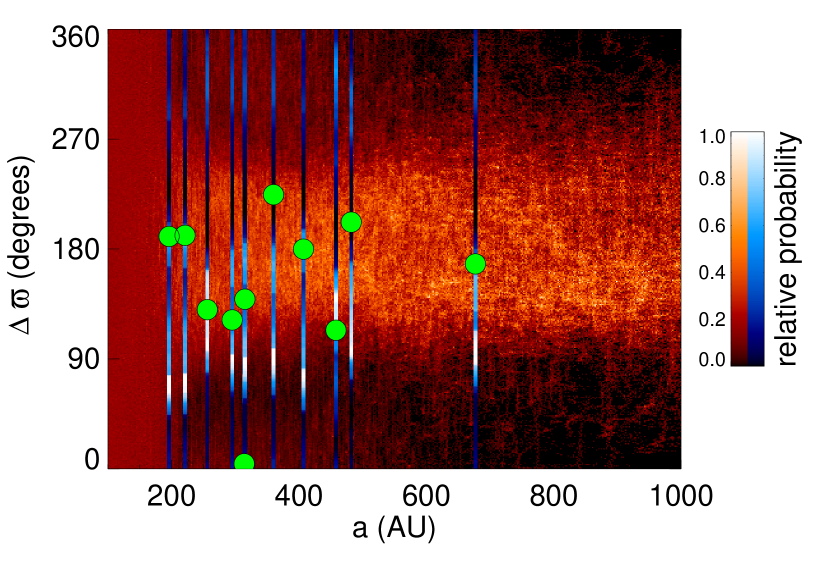
Figure 1: Semimajor axes versus $\varpi$ for the 11 KBOs of our sample (green points). The points are plotted as $\Delta\varpi$, defined as $\varpi-\varpi_{9}$, where here we plot the points for an assumed value of $\varpi_{9}=254^{\circ}$. For each known distant KBO we show a one-dimensional projection of the bias with respect to $\varpi$ (blue). While consistent bias exists, the $\varpi$ cluster is approximately $90^{\circ}$ removed from the direction of bias. We also show the probability density of $\varpi$ versus semimajor axis in the maximum likelihood model with $m_{9}=5$ M_e, $a_{9}=300$ AU, $e_{9}=0.15$ and $i_{9}=16^{\circ}$ (red). The density plot is normalized at every semimajor axis to better show the longitudinal structure. Note that this comparison is simply for visualization; the full maximum-likelihood model compares the full set of orbit elements of each object to the simulations and also incorporates the observational biases on each observed objects.

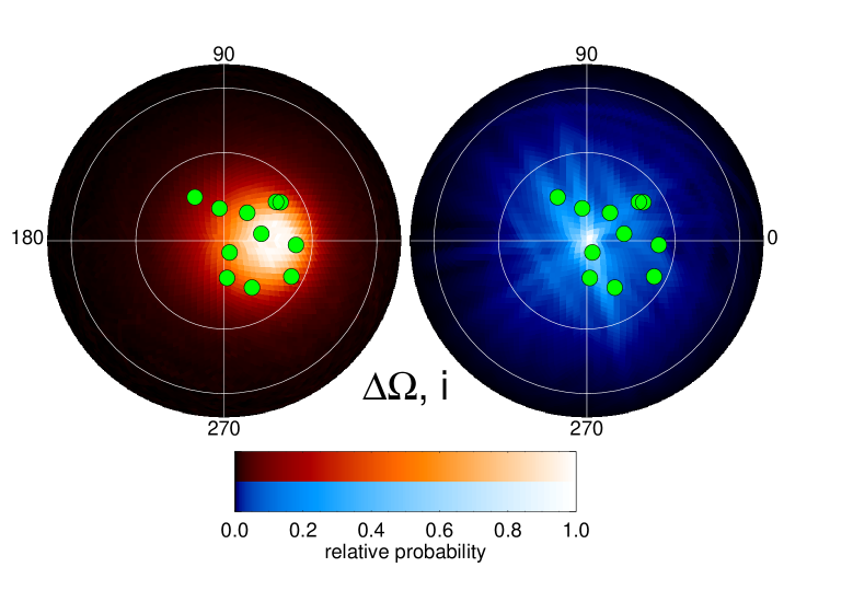
Figure 2: A comparison of the projection of the pole position of the distant detached KBOs (the green points show ($\sin i\cos\Delta\Omega$, $\sin i\sin\Delta\Omega$), where $\Delta\Omega$ is the difference between the longitude of ascending node of the observed object and of the modeled Planet Nine, assumed to be $108^{\circ}$ here) and a density plot of their expected values in the maximum likelihood model (red background). In blue we show an average of the two-dimensional projection of the pole position bias of all of the objects. While strong bias in pole position exists, no preferential direction is apparent. White circles indicate 30 and 60 degree inclinations.

Table 1: Orbital elements of all reported objects with $150<a<1000$ and $q>42$ AU.

name	a	e	i	$\Omega$	$\varpi$
	AU		deg.	deg.	deg.
2000CR105	218	0.80	22.8	128.3	85.0
2003VB12	479	0.84	11.9	144.3	95.8
2004VN112	319	0.85	25.6	66.0	32.8
2010GB174	351	0.86	21.6	130.8	118.2
2012VP113	258	0.69	24.1	90.7	24.2
2013FT28	312	0.86	17.3	217.8	258.3
2013RA109	458	0.90	12.4	104.7	7.5
2013SY99	694	0.93	4.2	29.5	61.6
2013UT15	197	0.78	10.7	192.0	84.1
2014SR349	302	0.84	18.0	34.8	15.7
2015RX245	412	0.89	12.1	8.6	73.7

Note. — As of 20 August 2021.

3 Bias

All telescopic surveys contain observational biases. Correctly understanding and implementing these biases into our modeling is critical to correctly using the observations to extract orbital parameters of Planet Nine. BB19 developed a method to use the ensemble of all known KBO detections to estimate a full geometric observational bias for individual distant KBOs. For each of the distant KBOs, they create the function

$$B_{j}^{(a,e,H)_{j}}[(i,\varpi,\Omega)|U],$$ (1)

where, for our case, $j$ represents one of the 11 distant KBOs of the sample and $B_{j}^{(a,e,H)_{j}}$ is the probability that distant KBO $j$, with semimajor axis, eccentricity, and absolute magnitude $(a,e,H)_{j}$ would be detected with orbital angles $i$, $\varpi$, and $\Omega$, if the population were uniformly distributed in the sky, given $U$, the ensemble of all known KBO detections. The details of the method are explained in BB19, but, in short, it relies on the insight that every detection of every KBO can be thought of (with appropriate caveats) as an observation at that position in the sky that could have detected an equivalent object $j$ with $(a,e,H)_{j}$ if, given the required orbital angles $(i,\varpi,\Omega)$ to put object $j$ at that position in the sky, the object would be predicted to be as bright as or brighter at that sky position than the detected KBO. For each sample object $j$ with $(a,e,H)_{j}$, the ensemble of all KBO detections can thus be used to estimate all of the orbital angles at which the object could have been detected. This collection of orbital angles at which an object with $(a,e,H)_{j}$ could have been detected represents the bias in $(i,\varpi,\Omega)$ for object $j$. While biases calculated with this method are strictly discrete, we smooth to one degree resolution in all parameters for later application to our dynamical simulations.

Note that this method differs from bias calculations using full survey simulators. It does not rely on knowledge of the survey details of the detections, but rather just the fact of the detection itself. Comparison of these bias calculations with the bias calculated from a full survey similar for the OSSOS survey shows comparable results (BB19).

Of the objects in our sample, all were included in the BB19 calculations with the exception of 2013 RA109, which had not been announced at the time of the original publication. We reproduce the algorithm of BB19 to calculate a bias probability function for this object.

While the bias is a separate 3-dimensional function for each object, we attempt to give an approximate visual representation of these biases in Figure 1, which collapses the bias of each object in $\varpi$ into a single dimension. As can be seen, a strong observational bias in $\varpi$ exists, but the observed clustering is approximately $90^{\circ}$ removed from the position of this bias. Figure 2 shows the bias in pole position. While, again, each object has an individual bias, the pole position biases are sufficiently similar that we simply show the sum of all of the biases, collapsed to two dimensions. Strong pole position biases exist, but none which appear capable of preferentially biasing the pole in any particular direction.

With the bias function now available, we re-examine the statistical significance of the angular clustering of the distant KBOs by updating the analysis of BB19 for the objects in our current analysis set. As in that analysis, we perform $10^{6}$ iterations where we randomly chose $(i,\varpi,\Omega)$ for the 11 objects of our sample assuming uniform distributions in $\varpi$ and $\Omega$ and a $\sin i\exp(-i^{2}/2\sigma^{2})$ distribution with $\sigma=16^{\circ}$ for $i$, and project these to the four-dimensional space of the canonical Poincaré variables $(x,y,p,q)$, corresponding roughly to longitude of perihelion ($x,y$) and pole position ($p,q$) (see BB19 for details). For each of the iterations we compute the average four-dimensional position of the 11 simulated sample objects and note whether or not this average position is more distant than the average position of the real sample. This analysis finds that the real data are more extreme than 99.6% of the simulated data, suggesting only a 0.4% chance that these data are selected from a random sample. Examination of Figures 1 and 2 give a good visual impression of why this probability is so low. The data are distributed very differently from the overall bias, contrary to expectations for a uniform sample.

The significance of the clustering retrieved here is slightly worse than that calculated by BB19. While one new distant object has been added to the sample, the main reason for the change in the significance is that, after the Batygin et al. (2019) analysis, we now understand much better which objects should most be expected to be clustered by Planet Nine, thus our total number of objects in our sample is smaller. Though this smaller sample leads to a slightly lower clustering significance, we nonetheless recommend the choice of $150<a<1000$ AU and $q>42$ AU for any analyses going forward including newly discovered objects.

With the reassurance that the clustering is indeed robust, we now turn to using the biases to help determine the orbital parameters of Planet Nine.

4 Planet Nine orbital parameter estimation

To estimate orbital parameters of Planet Nine, we require a likelihood model for a set of orbital parameters given the data on the observed distant KBOs. In practice, because of the structure of our bias calculations, which only account for on-sky geometric biases and do not attempt to explore biases in semimajor axis or perihelion, we reformulate this likelihood to be that of finding the observed value of ($i,\varpi,\Omega)_{j}$ given the specific value of $(a,e)_{j}$ for each distant object $j$. Conceptually, this can be thought of as calculating the probability that an object with a measured value of $a$ and a measured value of $q$ would be found to have the measured values of $i$, $\varpi$, and $\Omega$ for a given set of Planet Nine orbital parameters.

The random variables for this model are the mass of the planet, $m_{9}$, the semimajor axis, $a_{9}$, the eccentricity, $e_{9}$, the inclination, $i_{9}$, the longitude of perihelion, $\varpi_{9}$, and the longitude of ascending node, $\Omega_{9}$. As the effects of Planet Nine are now understood to be mainly secular (Beust, 2016), the position of Planet Nine within its orbit (the mean anomaly, $M_{9}$) does not affect the outcome, so it is unused. We thus write the likelihood function of the $j^{\rm th}$ KBO in our data set as:

$$\mathcal{L}_{j}^{(a,e)_{j}}[(m_{9},a_{9},e_{9},i_{9},\varpi_{9},\Omega_{9})|(i,\varpi,\Omega)_{j}],$$ (2)

where the $(a,e)_{j}$ superscript refers to the fixed value of $a$ and $e$ for object $j$. The full likelihood, $\mathcal{L}_{\rm P9}$ is the product of the individual object likelihoods. The likelihood of observing $(i,\varpi,\Omega)_{j}$ given a set of Planet Nine parameters depends on both the physics of Planet Nine and the observational biases.

4.1 Simulations

While $\mathcal{L}_{\rm P9}$ is presumably a continuous function of the orbital parameters, we must calculate the value at discrete locations using numerical simulations. We perform 121 of these simulations at manually chosen values of $m_{9}$, $a_{9}$, $e_{9}$, and $i_{9}$, as detailed below. The two angular parameters, $\varpi_{9}$ and $\Omega_{9}$, yield results that are rotationally symmetric so we need not individually simulate these results but rather rotate our reference frame to vary these parameters later. We set $M_{9}=0$ for the starting position of all simulations as this parameters does not affect the final orbital distributions.

To save computational time, previous Planet Nine simulations have often included only the effects of Neptune plus a $J_{2}$ term to simulate the combined orbit-averaged torque of the three inner gas giants. While this approach captures the relevant processes at the qualitative level, here, as we are interested in a detailed comparison with observations, we fully include all four inner giant planets. For each independent simulation a set of between 16,800 and 64,900 test particles is initially distributed with semimajor axis between 150 and 500 AU, perihelion between 30 and 50 AU, inclination between 0 and $25^{\circ}$, and all other orbital angles randomly distributed. The orbits of the 5 giant planets and test particles are integrated using the mercury6 gravitational dynamics software package (Chambers, 1999). To carry out the integrations we used the hybrid symplectic/Bulirsch-Stoer algorithm of the package, using a time step of 300 days which is adaptively reduced to directly resolve close encounters. Objects that collide with planets or reach $r<4.5$ or $r>10000$ AU are removed from the simulation for convenience. The orbital elements of all objects are defined in a plane in which the angles are referenced to the initial plane of the four interior giant planets. As Planet Nine precesses the plane of the planets, however, the fixed reference coordinate system no longer corresponds to the plane of the planets. Thus, after the simulations are completed, we recompute the time series of ecliptic-referenced angles by simply rotating to a coordinate system aligned with the orbital pole of Jupiter. In this rotation we keep the longitude zero-point fixed so that nodal precession of test particles and Planet Nine can be tracked.

A total of 121 simulations was performed, varying the mass ($m_{9}$), semimajor axis ($a_{9}$), eccentricity ($e_{9}$), and inclination ($i_{9}$). Parameters for Planet Nine were chosen by hand in an attempt to explore a wide range of parameter space and find the region of maximum likelihood. The full set of parameters explored can be seen in Table 2. Examination of the initial results from these simulations confirms the conclusions of Batygin et al. (2019): varying the orbital parameters of Planet Nine produces large effects on the distant Kuiper belt (Fig. 3). We see, for example, that fixing all parameters but increasing $m_{9}$ smoothly narrows the spread of the distant cluster (the feature labeled “cluster width” in Figure 3). Increasing $i_{9}$ smoothly moves the orbital plane of the clustered objects to follow the orbital plane of Planet Nine, until, at a values above $i_{9}~{}>30^{\circ}$, the increased inclination of Planet Nine tends to break the clustering entirely (Figure 4). Increasing $m_{9}$ also leads to a decrease in the distance to the transition between unclustered and clustered objects (the feature labeled the “wall” in Figure 3), while increasing the perihelion distance of Planet Nine ($q_{9}$) increases the distance to the wall. Many other more subtle effects can be seen in the full data set. While we point out all of these phenomena, our point is not to parameterize or make use of any of them, but rather to make the simple case that the specific orbital parameters of Planet Nine cause measurable effects on the distributions of objects in the distant Kuiper belt. Thus, we should be able to use the measured distributions to extract information about the orbital parameters of Planet Nine. We will accomplish this task through our full likelihood model.

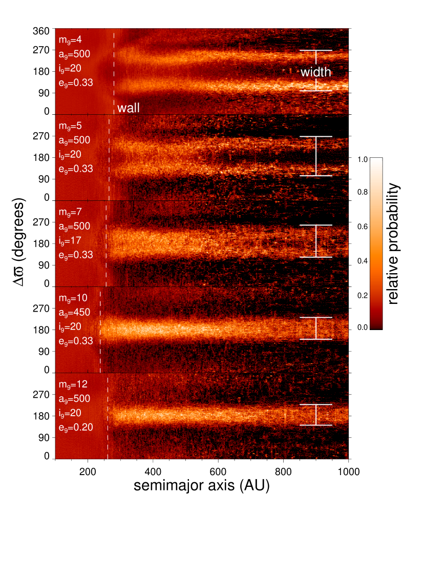
Figure 3: Probability density of $a$ versus $\Delta\varpi$ for a variety of simulated Planets Nine, in the same format as Fig.1. At the lowest masses the cluster appears double-peaked as the clustered objects librate and spend greater amounts of time at their inflection points. The dashed line labeled ”wall” shows the transition between the nearby uniform population and the more distant clustered population. This transition distance decrease with increasing $m_{9}$ and decreasing $a_{9}$ and $q_{9}$. The width of the cluster decreases with increasing $m_{9}$. Systematic changes such as these demonstrate that the orbital distribution of the distant KBOs is strongly influenced by the orbital parameters of Planet Nine.

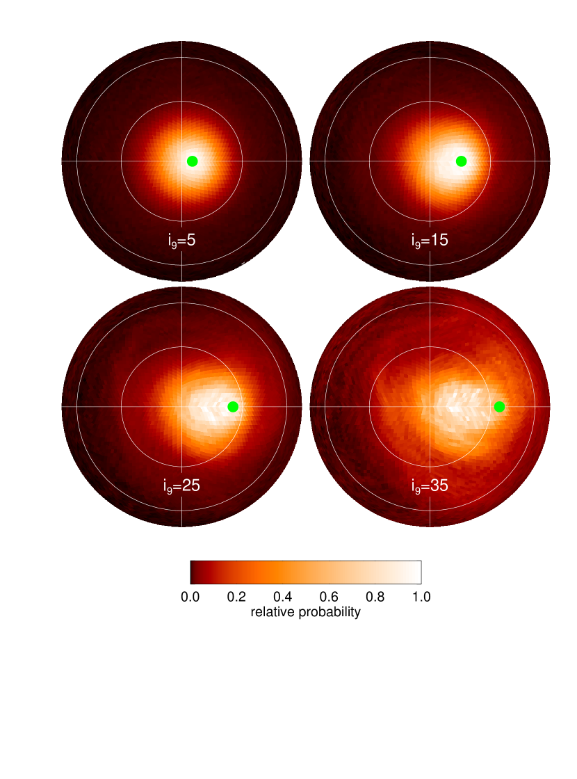
Figure 4: The probability distribution of the pole positions of KBOs with $a>150$ AU and $q>42$ AU for four Planet Nine models. All models have $m_{9}=7$ M_earth, $a_{9}=500$ AU, and $e_{9}=0.33$ and the effect of changing $i_{9}$ can be seen. The green dot shows the pole position of Planet Nine in the simulations. The white circle show 30 and 60^∘ inclinations. For small inclinations the distant KBOs track the inclination of Planet Nine. As $i_{9}$ increases, however, the overall longitudinal clustering diminishes and the pole positions cluster less tightly around that of Planet Nine.

4.2 Kernel density estimation

Each numerical simulation contains snapshots of the orbital distribution of the outer solar system for a finite number of particles. We use kernel density estimation to estimate a continuous function for the probability distribution function (PDF) from these discrete results of each simulation, that is, we seek the probability of observing an object at $(i,\varpi,\Omega)_{j}$ given $(a,e)_{j}$ for each simulation. The early times of the simulations contain a transient state that appears to reach something like a steady-state in orbital distribution after $\sim 1$ Gyr. We thus discard these initial time steps and only include the final 3 Gyr in our analysis. In all simulations the number of surviving objects continues to decrease with time, with a wide range in variation of the ejection rate that depends most strongly on P9 mass and perihelion distance.

For each numerical model, $k$, and each observed KBO, $j$, we repeat the following steps. First, we collect all modeled objects that pass within a defined smoothing range of $a_{j}$ and $q_{j}$, the parameters of the observed KBO. Because of our finite number of particles, smoothing is required to overcome the shot noise which would otherwise dominate the results. Based on our observation that the behaviour of the modeled KBOs changes rapidly with changing semimajor axis around the transition region (we do not know this transition region a priori but it is within 200-400 AU in all the simulations; see Figures 1 and 3, for example) but changes little at large semimajor axes, we define the smoothing range in $a$ as a constant value of 5% for $a_{j}<230$ AU, but, because the number of particles in the simulations declines with increasing semimajor axis, we allow the smoothing distance to linearly rise to 30% by $a_{j}=730$ AU. For perihelia beyond 42 AU, we observe little change in behaviour as a function of $q$, so we define a simple smoothing length of $q_{j}\pm 10$ AU with a lower limit of 42 AU (which is the limit we imposed on the observed KBOs). The main effect of these two smoothing parameters will be to slightly soften the sharp transition region (“the wall”) which, in practice, will contribute to the uncertainties in our derived mass, eccentricity, and, semimajor axis.

We select all of the modeled KBOs at times after the initial Gyr of simulation that pass within these $a$ and $q$ limits at any time step, and we weight them with two Gaussian kernels, each with a $\sigma$ equal to half of the smoothing distances defined above. The selected objects now all contain similar semimajor axis and perihelion distance as the $j^{\rm th}$ observed KBO, and their normalized distribution gives the probability that such an observed KBO would have a given inclination, longitude of perihelion, and longitude of ascending node. At this point the simulated values of $\varpi$ and $\Omega$ are all relative to $\varpi_{9}$ and $\Omega_{9}$, rather than in an absolute coordinate system. We refer to these relative values as $\Delta\varpi$ and $\Delta\Omega$.

We create the three-dimension probability distribution function of $(i,\Delta\varpi,\Delta\Omega)$ by selecting a value of $\Delta\varpi$ and then constructing a probability-distribution function of the pole position $(\sin i\cos\Omega,\sin i\sin\Omega)$, again using kernel density estimation now using a Gaussian kernel with $\sigma=2^{\circ}$ in great-circle distance from the pole position and $\sigma=10^{\circ}$ in longitudinal distance from $\Delta\varpi$ and multiplying by the $a,q$ weighting from above. In practice we grid our pole position distribution as a HEALPIX map (with NSIDE=32, for an approximately 1.8 degree resolution) and we calculate separate pole position distributions for each value of $\Delta\varpi$ at one degree spacings. This three-dimensional function is the probability that an unbiased survey that found a KBO with $a_{j}$ and $q_{j}$ would have found that object with $(i,\Delta\varpi,\Delta\Omega)_{j}$ in the $k^{th}$ simulation, or

$$P_{j,k}^{(a,e)_{j}}[(i,\Delta\varpi,\Delta\Omega)_{j}|(m_{9},a_{9},e_{9},i_{9})_{k}].$$ (3)

For arbitrary values of $\varpi_{9}$ and $\Omega_{9}$, this probability distribution can be translated to an absolute frame of reference with simple rotations to give

$$P_{j,k}^{(a,e)_{j}}[(i,\varpi,\Omega)_{j}|(m_{9},a_{9},e_{9},i_{9})_{k},\varpi_{9},\Omega_{9}].$$ (4)

4.3 Likelihood

With functions now specified for the probability of detecting object $j$ at $(i,\varpi,\Omega)_{j}$ and also for the probability of detecting object $j$ at $(i,\varpi,\Omega)_{j}$ assuming a uniform distribution across the sky, we can calculate our biased probability distribution for object $j$ in simulation $k$, $P^{\prime}_{j,k}$, by simple multiplication:

$$P_{j,k}^{\prime(a,e)_{j}}[(i,\varpi,\Omega)_{j}|(m_{9},a_{9},e_{9},i_{9})_{k},\varpi_{9},\Omega_{9}]=\\ P_{j,k}\times B_{j}^{(a,e,H)_{j}}[(i,\varpi,\Omega)_{j}|U]$$ (5)

where the arguments for $P_{j,k}$ are omitted for simplicity. We rewrite this probability as our likelihood function in the form of Equation (2) and take the product of the individual $j$ likelihoods to form the overall likelihood for each model $k$ at the values of $\varpi_{9}$ and $\Omega_{9}$:

$$\mathcal{L}_{k}[(m_{9},a_{9},e_{9},i_{9})_{k},\varpi_{9},\Omega_{9}|X],$$ (6)

where $X$ represents the full set of orbital elements of the distant KBOs from Table 2. The likelihood is discretely sampled by the numerical models in the first four parameters and continuously sampled analytically in the two angular parameters.

The likelihoods sparsely sample a seven-dimensional, highly-correlated parameter space. With even a cursory examination of the likelihoods, however, several trends are apparent (Figures 5 and 6). First, the model with the maximum likelihood, $M_{9}=5$ M_earth, $a_{9}=300$ AU, $i_{9}=17^{\circ}$, $e_{9}=0.15$, $\varpi_{9}=254^{\circ}$, and $\Omega_{9}=108^{\circ}$, is nearly a local peak in every dimension. Semimajor axes inside of $\sim$300 AU lead to low likelihoods, but more distant Planets Nine are viable (particularly if they are more massive), even if at reduced likelihood. The inclination appears quite well confined to regions near 15^∘, and strong peaks near $\varpi_{9}=250^{\circ}$ and $\Omega_{9}=100^{\circ}$ are evident.

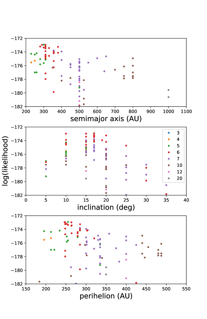
Figure 5: One dimensional plots of the log(likelihood) values as function of semimajor axis ($a_{9}$), inclination ($i_{9}$) and perihelion distance ($q_{9}$), at the maximum likelihood in $\Omega_{9}$ and $\varpi_{9}$ for each simulation. The points are colored by the mass of Planet Nine ($m_{9}$) as shown in the legend. The one-dimensional plots show the general behavior but do not show the significant correlations between parameters.

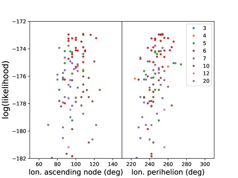
Figure 6: The longitude of ascending node ($\Omega_{9}$) and the longitude of perihelion ($\varpi_{9}$) at which the maximum likelihood occurs in each of the simulations. The points are colored by the mass of Planet Nine ($m_{9}$).

4.4 Gaussian process emulation

To further explore the orbital parameters, their correlations, and their uncertainties, we require a continuous, rather than discretely sampled, likelihood function. To estimate this likelihood at an arbitrary value of $(m_{9},a_{9},i_{9},e_{9},\varpi_{9},\Omega_{9})$ we perform the following steps. First, because the likelihoods as functions of $\varpi_{9}$ and $\Omega_{9}$ are densely sampled for each simulation, we perform a simple interpolation to obtain an estimated likelihood for each simulation at the specific desired value of $\varpi_{9}$ and $\Omega_{9}$. We next take the 121 simulations with their now-interpolated likelihoods and use these to create a computationally inexpensive Gaussian Process model as an emulator for the likelihoods. The behaviour of the likelihoods is extremely asymmetric, in particular in $m_{9}$ and $a_{9}$, with likelihood falling rapidly at small values of $m_{9}$ but dropping only slowly at higher values. Likewise, the likelihoods change rapidly for small values of $a_{9}$, while changing more slowly at higher $a_{9}$. To better represent this behaviour, we rescale the variables that we use in our Gaussian Process modeling. We use $a^{\prime}=(a_{9}/m_{9})^{-0.5}$ and we replace $e_{9}$ with a similarly-scaled function of perihelion distance, $q^{\prime}=\{a_{9}*(1-e_{9})/m_{9}\}^{-0.5}$. These scalings cause the likelihoods to appear approximately symmetric about their peak values and to peak at similar values of $a^{\prime}$ and $q^{\prime}$ for all masses (Figure 6). To enforce the smoothness and symmetry in the Gaussian Process model, we choose a Mateŕn kernel, which allows for a freely adjustable smoothness parameter, $\nu$. We chose a value of $\nu=1.5$, corresponding to a once-differentiable function, and which appears to adequately reproduce the expected behavior of our likelihood models. We force the length scales of the Matérn kernel to be within the bounds (0.5, 2.0), (0.02, 0.05), (1.0, 10.0), and (1.0,100.0) for our 4 parameters and for units of earth masses, AU, and degrees, corresponding to the approximate correlation length scales that we see in the likelihood simulations. We multiply this kernel by a constant kernel and also add a constant kernel. Beyond the domain of the simulations we add artificial points with low likelihood to prevent unsupported extrapolation. The model is implemented using scikit-learn in Python (Pedregosa et al., 2011).

The emulator produces a likelihood value at arbitrary values of $(M_{9},a_{9},i_{9},e_{9},\varpi_{9},\Omega_{9})$, and appears to do a reasonable job of reproducing the likelihoods of the numerical models, interpolating between these models, and smoothly extending the models over the full range of interest. Figure 7 gives an example of the correspondence between individual measured likelihoods and the emulator in the rescaled variable $a^{\prime}$. Viewed in the rescaled variables, the likelihoods and the emulator are relatively regular, symmetric, and well-behaved. Similar results are seen for $i_{9}$ and $q_{9}$. While the emulator does not perfectly reproduce the simulation likelihoods, the large-scale behavior is captured with sufficient fidelity to allow us to use these results for interpolation between the discrete simulations.

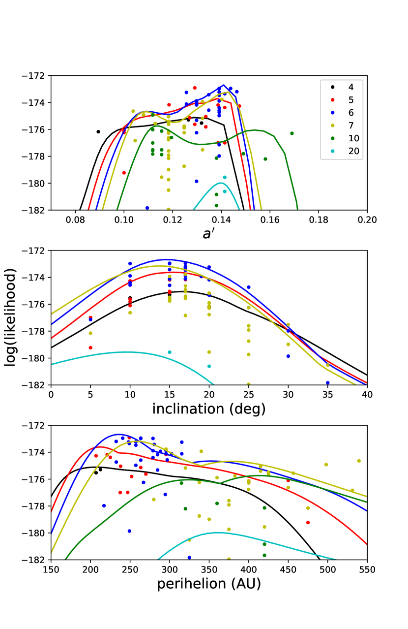
Figure 7: The discrete log(likelihoods) from the simulation versus the continuous results from the emulator. Results from different values of $m_{9}$ are shown as different colors and labeled in the legend. The top panel shows the rescaled parameter $a^{\prime}=(a_{9}/m_{9})^{-0.5}$. In this rescaled variable the likelihoods are approximately symmetric and vary smoothly as a function of mass different masses. The lines show the output from the Gaussian Process emulator with a fixed value of $i_{9}=15^{\circ}$, maximum likelihood values of $\Omega_{9}$ and $\varpi_{9}$ and an iterative search to find the maximum likelihood value for $e_{9}$. The emulator result shown thus represents the highest possible maximum likelihood at $i_{9}=15^{\circ}$ for each value of $a^{\prime}$ for each $m_{9}$. The middle panel shows emulator results versus inclination for the maximum likelihood values of all parameters, while the bottom panel shows emulator results versus perihelion at a fixed inclination of $i_{9}=15^{\circ}$ and maximum likelihood values of the other parameters. In all cases, the emulator output follows the upper envelope of the likelihoods, as expected.

4.5 MCMC

We use this Gaussian Process emulator to produce a Markov Chain Monte Carlo (MCMC) model of the mass and orbital parameters of Planet Nine. We use the Python package emcee (Foreman-Mackey et al., 2013) which implements the Goodman & Weare (2010) affine-invariant MCMC ensemble sampler. We consider two different priors for the semimajor axis distribution. The Planet Nine hypothesis is agnostic to a formation mechanism for Planet Nine, thus a uniform prior in semimajor axis seems appropriate. Nonetheless, different formation mechanisms produce different semimajor axis distributions. Of the Planet Nine formation mechanisms, ejection from the Jupiter-Saturn region followed by cluster-induced perihelion raising is the most consistent with known solar system constraints (Batygin et al., 2019). In Batygin & Brown (2021) we consider this process and find a distribution of expected semimajor axes that smoothly rises from about 300 AU to a peak at about 900 AU before slowly declining. The distribution from these simulations can be empirically fit by a Fréchet distribution of the form $p(a)=(a-\mu)^{-(\alpha+1)}\exp(-((a-\mu)/\beta)^{-\alpha})$ with $\alpha=1.2$, $\beta=1570$ AU, and $\mu=-70$ AU. We consider both this and the uniform prior and discuss both below. Additionally, we assume priors of $\sin(i_{9})$ in inclination and $e_{9}$ in eccentricity to account for phase-space volume. Priors in the other parameters are uniform. We sample parameter space using 100 separate chains (“walkers”) with which we obtain 20890 samples each. We use the emcee package to calculate the autocorrelation scales of these chains and find that maximum is 130 steps, which is 160 times smaller than the length of the chain, ensuring that the chains have converged. We discard the initial 260 steps of each chain as burn-in and sample each every 42 steps to obtain 49100 uncorrelated samples.

Examining the two different choices of prior for $a_{9}$ we see that the posterior distributions of the angular parameters, $i_{9}$, $\Omega_{9}$, and $\varpi_{9}$, are unchanged by this choice. The parameters $m_{9}$, $a_{9}$, and $e_{9}$ are, however, affected. This effect can best be seen in the posterior distributions of $a_{9}$ for the two different priors. The uniform prior has 16th, 50th, and 84th percentile values of $a_{9}=300$, 380, and 520 AU ($380^{+140}_{-80}$ AU) versus $a_{9}=360$, 460, and 640 AU ($460_{-100}^{+180}$ AU) for the cluster scattering prior. While the two posterior distributions agree within $1\sigma$, the differences are sufficiently large that predictions of expected magnitude, for example, could be affected. Here we will retain the uniform prior for continued analysis, but we keep in mind below the effects of a semimajor axis distribution with values approximately 20% larger. For this uniform prior, the marginalized perihelion and aphelion distances of Planet Nine are $300^{+85}_{-60}$ and $460^{+200}_{-110}$ AU, respectively.

Figure 8 shows a corner plot illustrating the full two-dimensional correlation between the posterior distribution of pairs of parameters for the cluster scattering prior in $a_{9}$. We see the clear expected correlations related to $a_{9}$, $m_{9}$, and $e_{9}$. No strong covariances exist between the other parameters. The posterior distributions for $i_{9}$ and $\Omega_{9}$ are among the most tightly confined, suggesting that the data strongly confine the pole position – and thus orbital path through the sky – of Planet Nine.

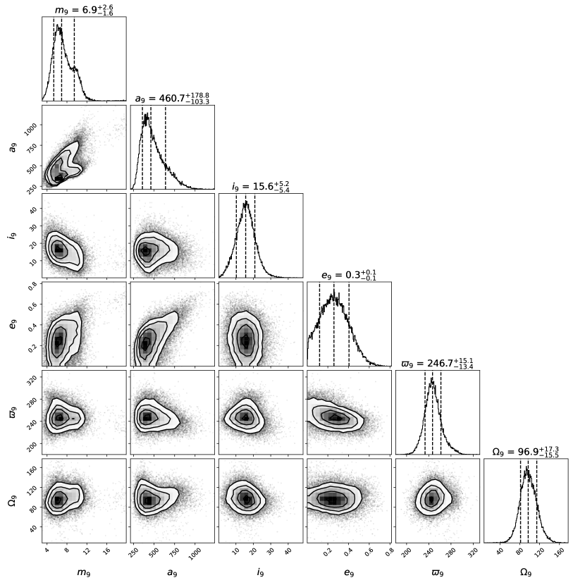
Figure 8: A corner plot showing the histograms and covariances of the parameters. The dashed lines on the histograms show the median and 16th and 84th percentiles of each marginalized distribution. The two dimensional histograms include the 1, 2, and 3$\sigma$ contour lines.

Examination of Fig. 1 helps to explain why low values of $m_{9}$ and $a_{9}$ are preferred. The mass is directly related to the width of the cluster, and masses greater than 6 M_earth lead to narrower clusters than those observed. Likewise, a low $m_{9}$ planet requires a small semimajor axis to have a distance to the wall of only $\sim$200 AU as the data appear to support. It is possible, of course, that the two KBOs with $a\sim 200$ AU are only coincidentally situated within the cluster and the real wall, and thus $a_{9}$ is more distant, but the likelihood analysis correctly accounts for this possibility.

5 The predicted position and brightness of Planet Nine

With distributions for the mass and orbital elements of Planet Nine now estimated, we are capable of determining the probability distribution of the on-sky location, the heliocentric distance, and the predicted brightness of Planet Nine. We first use the full set of samples from the MCMC to determine the probability distribution function of the sky position and heliocentric distance of Planet Nine. To do so we calculate the heliocentric position of an object with the orbital parameters of each MCMC sample at one degrees spacings in mean anomaly, $M_{9}$. The sky density of these positions is shown in Figure 9. Appropriately normalized, this sky plane density represents the probability distribution function of finding Planet Nine at any heliocentric position in the sky. Approximately 95% of the probability is within a swath of the sky that is $\pm 12^{\circ}$ in declination from an orbit with an inclination of $16\circ$ and an ascending node of$97^{\circ}$, the median marginalized values of these parameters.

Figure 9: The sky plane density, heliocentric distance, and predicted $R$ magnitude for our Planet Nine samples. The top panel is a Mollweide equal area projection centered at an RA of 180 and declination of 0. Thick lines show the celestial equator, the ecliptic, and $\pm 20^{\circ}$ from the galactic plane. Thin lines show every 45^∘ of RA and declination. The middle panel shows the probability distribution of heliocentric distance as a function of RA. The lines show the 16th, 50th, and 84th percentiles of the distribution. The bottom panel shows modeled R-band magnitudes again with the 16th, 50th, and 84th percentile distributions.The peak in probability density at R.A.$\sim 45$ corresponds to the predicted aphelion position of P9 where an eccentric object spends more of its time.

To estimate the magnitude of Planet Nine we need not just the mass, but also the diameter and the albedo, neither of which we directly constrain. We thus model what we consider to be reasonable ranges for these parameters.

For masses between 4-20 M_earth we assume that the most likely planetary composition is that of a sub-Neptune, composed of an icy-rocky core with a H-He rich envelope (we discuss alternatives below). We assume a simple mass-diameter relationship of $r_{9}=(m_{9}/{3\rm M}_{\rm earth})$ R_earth based on fits to (admittedly much warmer) planets in this radius and mass range by Wu & Lithwick (2013). The albedo of such an object has been modeled by Fortney et al. (2016), who find that all absorbers are condensed out of the atmosphere and the planet should have a purely Rayleigh-scattering albedo of $\sim$0.75. We conservatively assume a full range of albedos from 0.2 – half that of Neptune – to 0.75. With these diameters and albedos we can use the modeled distances to determine the brightness of Planet Nine for each of the samples. Figure 8 shows the predicted magnitudes of Planet Nine. At the brightest end, Planet Nine could already have been detected in multiple surveys, while at the faintest it will require dedicated searches on 8-10 meter telescopes.

6 Caveats

Both the maximum likelihood and the fully marginalized MCMC posterior distributions suggest that Planet Nine might be closer and potentially brighter than previously expected. The original analysis of Batygin & Brown (2016) was a simple proof-of-concept that an inclined eccentric massive planet could cause outer solar system clustering, so the choice of $m_{9}$=10 $M_{\rm earth}$, $e_{9}$=0.7, and $i_{9}=30^{\circ}$ was merely notional. Brown & Batygin (2016) showed that a wide range of masses and semimajor axes were acceptable with the constraints available at the time, while Batygin et al. (2019) showed hints of a preference for lower mass and semimajor axis. As previously discussed, one of the strongest drivers for the lower mass and semimajor axis of Planet Nine is the width of the longitude of perihelion cluster. With longitudes of perihelion ranging from 7 to 118^∘, this 111^∘ wide cluster is best matched by low masses, which necessitates low semimajor axes to bring the wall in as close as 200 AU.

One possibility for artificially widening the longitude of perihelion cluster is contamination by objects recently scattered into the $150<a<1000$ AU, $q>42$ AU region. It is plausible that 2013FT28, the major outlier outside of the cluster, is one such recently Neptune-scattered object. While integration of the orbit of 2013FT28 shows that it is currently metastable, with a semimajor axis that diffuses on $\sim$Gyr timescales, and while we attempted to exclude all recent Neptune-scattered objects by requiring $q>42$ AU, we nonetheless note that within the 200 Myr of our simulations $\sim$20% of the objects that start as typical scattering objects with $30<q<36$ AU and $a<150$AU have diffused to the $q>42$ AU, $a>150$ AU region. These diffusing objects are broadly clustered around $\Delta\varpi\sim 0\circ$ instead of around $\Delta\varpi\sim 180^{\circ}$ like the stable cluster. 2013FT28 is such a strong outlier, however, that whether it is a contaminant from this route or not, its presence has little affect on our final retrieved orbital parameters. No Planet Nine simulations are capable of bringing it into a region of high likelihood.

A more worrisome possibility for inflating the width of the longitude of perihelion clustering is the scattering inward of objects from the inner Oort cloud (Batygin & Brown, 2021). As noted earlier, we have no clear way to discriminate against these objects, and while the most distant objects are more likely to have originated from this exterior source, such objects can be pulled down to small semimajor axes, too. We have no understanding of the potential magnitude – if any – of this potential contaminating source, so we assess the maximum magnitude of the effect by systematically examining the exclusion of objects from the data set. Limiting the number of objects under consideration will necessarily raise the uncertainties in the extracted parameters, but we instead here simply look at how it changes the maximum likelihood simulation.

We recalculate the maximum likelihood values of each simulation after exclusion of the object most distant from the average $\varpi$ position of the cluster (with the exception of 2013FT29, which we always retain). Even after excluding the 6 most extreme objects in the cluster and retaining only 4, the maximum likelihood changes only from $m_{9}=5$ to $m_{9}=6$ M_⊕ and from $a_{9}=300$ to $a_{9}=310$ AU. The orbital angles do not change substantially.

We conclude that the preference for smaller values of mass and semimajor axis is robust, and that the orbital angles ($i_{9},\Omega_{9},\varpi_{9}$) are largely unaffected by any contamination. While the posterior distributions for $m_{9}$ and $a_{9}$ have large tails towards larger values, the possibility of a closer brighter Planet Nine needs to be seriously considered.

An additional uncertainty worth considering is the diameter and albedo of Planet Nine. We have assumed values appropriate for a gas-rich sub-Neptune which, a priori, seems the most likely state for such a distant body. Given our overall ignorance of the range of possibilities in the outer solar system, we cannot exclude the possibility of an icy body resembling, for example, a super-Eris. Such an icy/rocky body could be $\sim$50% smaller than an equivalent sub-Neptune in this mass range (Lopez & Fortney, 2014), and while the large KBOs like Eris have high albedos, much of this elevated albedo could be driven by frost covering of darker irradiated materials as the objects move through very different temperature regimes on very eccentric orbits. An object at the distance of Planet Nine – which stays below the condensation temperature of most volatiles at all times – could well lack such volatile recycling and could have an albedo closer to the $\sim$10% of the large but not volatile-covered KBOs (Brown, 2008). Overall the effect of a smaller diameter and smaller albedo could make Planet Nine $\sim$ 3 magnitudes dimmer. Such a situation would make the search for Planet Nine considerably more difficult. While the possibility of a dark super-Eris Planet Nine seems unlikely, it cannot be excluded.

Finally, we recall the affect of the choice of the prior on $a_{9}$. A prior assuming formation in a cluster would put Planet Nine more distant than shown here, though it would also predict higher masses. Combining those effects we find that the magnitude distribution seen in Figure 8 would shift fainter by about a magnitude near aphelion but would change little close to perihelion.

While all of these caveats affect the distance, mass, and brightness of Planet Nine, they have no affect on the sky plane position shown in Figure 8. To a high level of confidence, Planet Nine should be found along this delineated path.

7 Conclusion

We have presented the first estimate of Planet Nine’s mass and orbital elements using a full statistical treatment of the likelihood of detection of the 11 objects with $150<a<1000$ AU and $q>42$ AU as well as the observational biases associated with these detections. We find that the median expected Planet Nine semimajor axis is significantly closer than previously understood, though the range of potential distances remains large. At its brightest predicted magnitude, Planet Nine could well be in range of the large number of sky surveys being performed with modest telescope, so we expect that the current lack of detection suggests that it is not as the brightest end of the distribution, though few detailed analysis of these surveys has yet been published.

Much of the predicted magnitude range of Planet Nine is within the single-image detection limit of the LSST survey of the Vera Rubin telescope, $r\sim 24.3$, though the current survey plan does not extend as far north as the full predicted path of Planet Nine. On the faint end of the distribution, or if Planet Nine is unexpectedly small and dark, detection will still require imaging with 10-m class telescopes or larger.

Despite recent discussions, statistical evidence for clustering in the outer solar system remains strong, and a massive planet on a distant inclined eccentric orbit remains the simplest hypothesis. Detection of Planet Nine will usher in a new understanding of the outermost part of our solar system and allow detailed study of a fifth giant planet with mass common throughout the galaxy.

$m_{9}$	$a_{9}$	$i_{9}$	$e_{9}$	$\varpi_{9}$	$\Omega_{9}$	$\ell$	$\Delta\ell$	num.
($M_{\rm earth}$)	(AU)	(deg)		(deg)	(deg)			particles
3	625	15	0.60	356	166	-182.1	-9.2	21100
4	230	10	0.15	250	108	-175.5	-2.6	30000
4	250	15	0.15	260	102	-175.3	-2.4	30000
4	500	20	0.33	224	86	-176.2	-3.3	120500
5	230	10	0.15	246	96	-174.3	-1.4	30000
5	250	5	0.15	250	126	-177.0	-4.1	30000
5	250	10	0.15	248	108	-174.4	-1.5	30000
5	260	15	0.10	246	94	-174.2	-1.3	25600
5	260	5	0.15	246	82	-177.0	-4.1	30000
5	280	10	0.10	246	96	-175.8	-2.9	25600
5	280	15	0.10	266	88	-175.0	-2.1	25600
5	300	10	0.15	234	108	-175.6	-2.7	25600
5	300	17	0.15	254	108	-172.9	0.0	25600
5	310	15	0.10	274	102	-175.1	-2.2	25600
5	356	17	0.20	252	88	-174.2	-1.3	25600
5	500	5	0.33	250	96	-179.2	-6.3	25600
5	500	10	0.33	244	86	-176.1	-3.2	25500
5	500	20	0.33	234	86	-176.2	-3.3	20200
5	720	20	0.65	234	96	-185.1	-12.2	30100
6	280	17	0.10	256	100	-173.2	-0.3	25500
6	290	17	0.15	250	108	-173.0	-0.0	25600
6	300	17	0.15	246	100	-173.4	-0.4	25600
6	310	10	0.10	252	96	-174.4	-1.5	25600
6	310	15	0.10	256	96	-174.6	-1.7	25600
6	310	17	0.10	244	108	-175.0	-2.1	25600
6	310	10	0.15	256	108	-173.0	-0.1	25600
6	310	15	0.15	252	116	-173.0	-0.1	25600
6	310	17	0.15	266	106	-173.5	-0.6	19900
6	310	5	0.20	244	108	-177.1	-4.2	25600
6	310	10	0.20	244	108	-173.9	-1.0	25000
6	310	15	0.20	252	92	-173.0	-0.0	25400
6	310	17	0.20	260	122	-173.2	-0.3	13600
6	310	20	0.20	242	96	-173.2	-0.3	23700
6	310	25	0.20	230	92	-174.7	-1.8	20000
6	310	30	0.20	238	88	-178.0	-5.1	25500
6	330	10	0.20	248	108	-174.6	-1.7	31300
6	330	15	0.20	252	92	-173.4	-0.5	14400
6	356	20	0.10	254	100	-175.3	-2.4	25600
6	356	20	0.15	250	110	-174.2	-1.3	25600
6	356	15	0.20	256	102	-174.1	-1.2	21200
6	356	17	0.20	262	100	-174.1	-1.2	25600
6	356	17	0.20	264	108	-173.9	-1.0	25600
6	356	19	0.20	238	100	-173.9	-1.0	48500
6	356	25	0.20	228	88	-176.2	-3.3	40200
6	356	30	0.20	238	96	-179.9	-6.9	16700
6	380	17	0.20	242	110	-174.1	-1.2	25600
6	380	17	0.25	246	92	-173.3	-0.3	25600
6	500	35	0.15	242	96	-181.8	-8.9	30000
6	600	40	0.15	260	94	-184.0	-11.1	30000
6	800	50	0.15	242	82	-188.4	-15.5	30000
7	356	17	0.20	246	92	-173.8	-0.9	25600
7	400	15	0.25	254	82	-173.9	-1.0	30900
7	400	20	0.25	246	102	-175.2	-2.3	52800
7	400	30	0.25	230	88	-177.5	-4.6	30800
7	450	25	0.15	248	108	-178.7	-5.8	30000
7	450	15	0.33	250	86	-175.8	-2.8	29700
7	450	20	0.33	236	80	-175.9	-3.0	25600
7	450	25	0.33	236	80	-176.2	-3.3	23500
7	500	20	0.15	256	94	-176.3	-3.4	25600
7	500	15	0.20	256	102	-175.6	-2.7	25600
7	500	17	0.20	268	96	-175.1	-2.1	25600
7	500	25	0.20	254	92	-177.6	-4.7	25600
7	500	20	0.25	260	94	-176.8	-3.9	25600
7	500	5	0.33	242	96	-178.2	-5.2	57300
7	500	10	0.33	252	92	-176.6	-3.7	41400
7	500	15	0.33	250	98	-175.5	-2.6	47700
7	500	17	0.33	250	100	-175.4	-2.5	17500
7	500	20	0.33	242	86	-176.1	-3.2	52400
7	500	25	0.33	234	86	-177.9	-5.0	54000
7	500	30	0.33	232	94	-179.0	-6.1	59600
7	500	35	0.33	230	86	-180.5	-7.6	41700
7	500	25	0.40	228	86	-179.7	-6.8	35000
7	500	25	0.45	226	74	-182.0	-9.0	27700
7	525	20	0.50	236	70	-179.6	-6.6	33000
7	550	17	0.40	244	88	-175.6	-2.6	25600
7	600	17	0.45	238	94	-174.9	-2.0	25600
7	640	17	0.50	240	102	-176.8	-3.9	16900
7	650	17	0.45	230	88	-174.6	-1.7	25500
7	800	50	0.15	310	50	-190.4	-17.5	30000
7	830	20	0.70	208	96	-184.7	-11.7	51200
7	1000	60	0.15	298	94	-191.2	-18.3	30000
8	400	20	0.15	248	108	-177.1	-4.2	30000
10	350	10	0.15	250	96	-176.3	-3.4	30000
10	400	20	0.15	242	84	-178.2	-5.3	30000
10	450	20	0.33	242	82	-177.8	-4.9	34300
10	525	20	0.15	264	106	-178.1	-5.2	30000
10	525	30	0.15	266	102	-184.6	-11.7	30000
10	525	40	0.15	304	138	-189.9	-17.0	30000
10	525	20	0.50	244	114	-180.8	-7.9	39700
10	525	20	0.65	242	90	-181.7	-8.8	20900
10	525	30	0.65	244	36	-187.1	-14.2	35600
10	700	20	0.35	244	108	-176.6	-3.7	25600
10	700	30	0.70	290	132	-190.0	-17.1	25600
10	750	10	0.35	234	106	-177.5	-4.6	19500
10	750	15	0.35	252	114	-176.1	-3.2	22400
10	750	20	0.35	244	100	-177.9	-5.0	25500
10	800	5	0.40	244	114	-177.5	-4.6	25600
10	800	10	0.40	240	112	-177.0	-4.1	25600
10	800	15	0.40	240	118	-177.8	-4.9	25600
10	800	15	0.45	240	120	-174.9	-2.0	25600
10	800	20	0.45	238	108	-176.0	-3.1	28600
10	800	25	0.45	234	100	-177.6	-4.7	23500
10	800	30	0.45	242	50	-184.0	-11.1	16800
10	800	60	0.45	182	114	-183.0	-10.1	30400
10	870	20	0.73	254	92	-185.4	-12.5	17900
10	1000	60	0.15	314	96	-192.8	-19.9	23600
10	1400	70	0.15	224	30	-190.0	-17.1	30000
12	500	15	0.20	256	94	-178.4	-5.5	25600
12	500	20	0.20	256	92	-181.2	-8.3	25600
12	500	25	0.20	266	102	-182.9	-10.0	25600
12	920	20	0.73	224	76	-182.1	-9.1	25800
12	960	20	0.79	242	54	-186.8	-13.9	24900
14	960	20	0.74	220	76	-185.6	-12.7	28000
16	1000	20	0.75	248	76	-183.2	-10.2	33600
20	900	60	0.15	306	66	-189.0	-16.1	30000
20	1000	15	0.65	242	122	-179.6	-6.7	30100
20	1000	20	0.65	240	118	-180.6	-7.7	33000
20	1000	25	0.65	246	70	-185.5	-12.6	32300
20	1070	20	0.77	240	124	-185.2	-12.3	64900
20	1400	70	0.15	264	0	-186.8	-13.9	30000
20	2000	80	0.15	260	152	-190.1	-17.2	30000

Note. — Parameters used in the numerical simulations on the effects of Planet Nine ($m_{9}$, $a_{9}$, $i_{9}$, $e_{9}$) and the maximum ln(likelihood), $\ell$, which occurs at the listed value of $\varpi_{9}$ and $\Omega_{9}$. $\Delta\ell$ gives the difference in ln(likelihood) from the maximum value, which occurs at $m_{9}=5$, $a_{9}=310$, $i_{9}=15$, and $e_{9}=0.10$.

References

- Astropy Collaboration et al. (2013) Astropy Collaboration, Robitaille, T. P., Tollerud, E. J., et al. 2013, A&A, 558, A33, doi: 10.1051/0004-6361/201322068
- Bailey et al. (2018) Bailey, E., Brown, M. E., & Batygin, K. 2018, AJ, 156, 74, doi: 10.3847/1538-3881/aaccf4
- Bannister et al. (2017) Bannister, M. T., Shankman, C., Volk, K., et al. 2017, AJ, 153, 262, doi: 10.3847/1538-3881/aa6db5
- Batygin et al. (2019) Batygin, K., Adams, F. C., Brown, M. E., & Becker, J. C. 2019, Phys. Rep., 805, 1, doi: 10.1016/j.physrep.2019.01.009
- Batygin & Brown (2016) Batygin, K., & Brown, M. E. 2016, AJ, 151, 22, doi: 10.3847/0004-6256/151/2/22
- Batygin & Brown (2021) —. 2021, ApJ, 910, L20, doi: 10.3847/2041-8213/abee1f
- Bernardinelli et al. (2020) Bernardinelli, P. H., Bernstein, G. M., Sako, M., et al. 2020, The Planetary Science Journal, 1, 28, doi: 10.3847/PSJ/ab9d80
- Beust (2016) Beust, H. 2016, A&A, 590, L2, doi: 10.1051/0004-6361/201628638
- Brasser et al. (2012) Brasser, R., Duncan, M. J., Levison, H. F., Schwamb, M. E., & Brown, M. E. 2012, Icarus, 217, 1, doi: 10.1016/j.icarus.2011.10.012
- Brown (2008) Brown, M. E. 2008, in The Solar System Beyond Neptune, ed. M. A. Barucci, H. Boehnhardt, D. P. Cruikshank, & A. Morbidelli, 335–344
- Brown (2017) —. 2017, AJ, 154, 65, doi: 10.3847/1538-3881/aa79f4
- Brown & Batygin (2016) Brown, M. E., & Batygin, K. 2016, ApJ, 824, L23, doi: 10.3847/2041-8205/824/2/L23
- Brown & Batygin (2019) —. 2019, AJ, 157, 62, doi: 10.3847/1538-3881/aaf051
- Brown et al. (2004) Brown, M. E., Trujillo, C., & Rabinowitz, D. 2004, ApJ, 617, 645, doi: 10.1086/422095
- Chambers (1999) Chambers, J. E. 1999, MNRAS, 304, 793, doi: 10.1046/j.1365-8711.1999.02379.x
- Emel’yanenko et al. (2003) Emel’yanenko, V. V., Asher, D. J., & Bailey, M. E. 2003, MNRAS, 338, 443, doi: 10.1046/j.1365-8711.2003.06066.x
- Foreman-Mackey (2016) Foreman-Mackey, D. 2016, The Journal of Open Source Software, 1, 24, doi: 10.21105/joss.00024
- Foreman-Mackey et al. (2013) Foreman-Mackey, D., Hogg, D. W., Lang, D., & Goodman, J. 2013, Publications of the Astronomical Society of Pacific, 125, 306, doi: 10.1086/670067
- Fortney et al. (2016) Fortney, J. J., Marley, M. S., Laughlin, G., et al. 2016, ApJ, 824, L25, doi: 10.3847/2041-8205/824/2/L25
- Gladman et al. (2002) Gladman, B., Holman, M., Grav, T., et al. 2002, Icarus, 157, 269, doi: 10.1006/icar.2002.6860
- Gomes et al. (2006) Gomes, R. S., Matese, J. J., & Lissauer, J. J. 2006, Icarus, 184, 589, doi: 10.1016/j.icarus.2006.05.026
- Gomes et al. (2015) Gomes, R. S., Soares, J. S., & Brasser, R. 2015, Icarus, 258, 37, doi: 10.1016/j.icarus.2015.06.020
- Goodman & Weare (2010) Goodman, J., & Weare, J. 2010, Communications in applied mathematics and computational science, 5, 65
- Gorski et al. (2005) Gorski, K. M., Hivon, E., Banday, A. J., et al. 2005, The Astrophysical Journal, 622, 759–771, doi: 10.1086/427976
- Lawler et al. (2017) Lawler, S. M., Shankman, C., Kaib, N., et al. 2017, AJ, 153, 33, doi: 10.3847/1538-3881/153/1/33
- Lopez & Fortney (2014) Lopez, E. D., & Fortney, J. J. 2014, ApJ, 792, 1, doi: 10.1088/0004-637X/792/1/1
- Malhotra et al. (2016) Malhotra, R., Volk, K., & Wang, X. 2016, ApJ, 824, L22, doi: 10.3847/2041-8205/824/2/L22
- Millholland & Laughlin (2017) Millholland, S., & Laughlin, G. 2017, AJ, 153, 91, doi: 10.3847/1538-3881/153/3/91
- Morbidelli & Levison (2004) Morbidelli, A., & Levison, H. F. 2004, AJ, 128, 2564, doi: 10.1086/424617
- Napier et al. (2021) Napier, K. J., Gerdes, D. W., Lin, H. W., et al. 2021, arXiv e-prints, arXiv:2102.05601. https://arxiv.org/abs/2102.05601
- Pedregosa et al. (2011) Pedregosa, F., Varoquaux, G., Gramfort, A., et al. 2011, Journal of Machine Learning Research, 12, 2825
- Schwamb et al. (2010) Schwamb, M. E., Brown, M. E., Rabinowitz, D. L., & Ragozzine, D. 2010, ApJ, 720, 1691, doi: 10.1088/0004-637X/720/2/1691
- Shankman et al. (2017) Shankman, C., Kavelaars, J. J., Bannister, M. T., et al. 2017, AJ, 154, 50, doi: 10.3847/1538-3881/aa7aed
- Trujillo & Sheppard (2014) Trujillo, C. A., & Sheppard, S. S. 2014, Nature, 507, 471, doi: 10.1038/nature13156
- Wu & Lithwick (2013) Wu, Y., & Lithwick, Y. 2013, ApJ, 772, 74, doi: 10.1088/0004-637X/772/1/74