Temporal Network Embedding via Tensor Factorization

Abstract.

Representation learning on static graph-structured data has shown a significant impact on many real-world applications. However, less attention has been paid to the evolving nature of temporal networks, in which the edges are often changing over time. The embeddings of such temporal networks should encode both graph-structured information and the temporally evolving pattern. Existing approaches in learning temporally evolving network representations fail to capture the temporal interdependence. In this paper, we propose Toffee, a novel approach for temporal network representation learning based on tensor decomposition. Our method exploits the tensor-tensor product operator to encode the cross-time information, so that the periodic changes in the evolving networks can be captured. Experimental results demonstrate that Toffee outperforms existing methods on multiple real-world temporal networks in generating effective embeddings for the link prediction tasks.

1. Introduction

Network data has gained increasing popularity due to its ubiquitous applications in multiple domains, including recommendation systems, knowledge base, and biological informatics. Learning effective embeddings over network data involves efficiently projecting the structural properties of the network data into low-dimensional feature representations which can be further utilized by many downstreaming tasks, such as node label classification, link prediction, community detection and network reconstruction. The proposal of DeepWalk (Perozzi et al., 2014) has inspired the development of many network embedding techniques (Tang et al., 2015; Grover and Leskovec, 2016; Cao et al., 2015; Qiu et al., 2018). However, these techniques are all designed for static networks. While in most real-world applications, networks are usually dynamic and evolve over time. For example, in a social network, users’ friend relations tend to change over time, which alters the low-dimensional feature representation. Similarly, in a co-authorship network, authors’ relationship will fluctuate from time to time according to their new research projects. Therefore, it is essential to encode the temporal information into the network representation to improve the predictive power.

To capture the evolving pattern and the temporal interaction between nodes, several temporal network embedding algorithms have been proposed. (Nguyen et al., 2018) proposed CTDNE, a temporal version of random walks to capture the evolving graph structure. HTNE (Zuo et al., 2018) extended CTDNE by generating neighbors using the Hawkes process. (Qiu et al., 2020) proposed HNIP, a temporal random walk that preserves high-order proximity and used an auto-encoder to capture the nonlinearity of the network structure. All these neighborhood-based algorithms have an inherent disadvantage that their local structure inferences are heavily reliant on neighborhood relations and can overlook the global structure at large, which may incur poor performance especially when the graph is densely connected. This problem is further exacerbated for temporal network embedding. Besides, these methods lack interpretability, and require heavy tuning of hyper-parameters and model structures.

Tensors are an efficient way to model high-dimensional, multi-aspect data, such as spatio-temporal data (Zhu et al., 2016; Gauvin et al., 2014), where the spatial distribution at a specific timestamp will be modeled as a frontal slice of the tensor. Built on the success of the matrix factorization-based network embedding methods (Cao et al., 2015; Qiu et al., 2018) in revealing useful global structure information of the network, tensors are able to capture both the global network structure and the temporal node interactions at the same time. Due to the inefficacy of traditional tensor factorization approaches such as CANDECOMP/PARAFAC (CP) and Tucker decomposition to take advantage of the slice-wise correlations, RESCAL (Nickel et al., 2011) was proposed to learn representations of multi-relational data. Nonetheless, RESCAL is still insufficient in capturing the temporal evolution by a single embedding matrix.

In this paper, we propose a Tensor factorization algorithm for temporal network embedding (Toffee), which models the temporal network structure as a three-way tensor, and learns unique representations for the temporal network through a novel tensor factorization algorithm. Toffee is superior to RESCAL by capturing the cross-time relation. This is empowered by the tensor-tensor product (t-product) (Kilmer and Martin, 2011; Zhang et al., 2014), which has demonstrated great potential in image/video domain by exploiting the circular convolution operator along the temporal dimension.

We briefly summarize our contributions as follows. 1) We propose Toffee, a new tensor factorization model that incorporates the t-product for temporal network embedding. Toffee  manifests superior capability in capturing both the global structure information and the temporal interactions between nodes. 2) Toffee is able to extract unique representations for asymmetric relationships between nodes (both directed and indirected). 3) Experiments on multiple real-world network datasets show that Toffee is capable of generating embeddings with better predictive power compared to state-of-the-art approaches in temporal network embedding.

2. Preliminaries and Notations

In this section, we introduce the frequently used definitions and notations in this paper. We use $A$ to denote a matrix, $\bm{\mathscr{A}}$ to denote a tensor, and $\bm{\mathscr{A}}(i,:,:)$, $\bm{\mathscr{A}}(:,i,:)$, $\bm{\mathscr{A}}(:,:,i)$ denote the horizontal, lateral and frontal slice of tensor $\bm{\mathscr{A}}$, respectively. We use $\bm{\mathscr{A}}^{(i)}$ to represent $\bm{\mathscr{A}}(:,:,i)$. We denote $\bm{\mathscr{A}}_{\mathscr{F}}={\tt fft}(\bm{\mathscr{A}},[\hskip 2.84526pt],d)$ as the tensor after fast Fourier transform (fft) along the $d$-th mode, and $\bm{\mathscr{A}}_{\mathscr{F}}$ can be transformed back to $\bm{\mathscr{A}}$ through the inverse fft $\bm{\mathscr{A}}={\tt ifft}(\bm{\mathscr{A}}_{\mathscr{F}},[~{}],d)$.

Definition 2.1.

(Temporal Network) A temporal network $\bm{\mathscr{G}}$ is denoted as $\bm{\mathscr{G}}=(\bm{\mathscr{V}},\bm{\mathscr{E}},\bm{\mathscr{T}})$, where $\bm{\mathscr{V}}$ is a set of nodes, $\bm{\mathscr{E}}$ is the set of edges, and $\bm{\mathscr{T}}$ is the sequence of timestamps. Given $t\in\bm{\mathscr{T}}$, we will have a sequence of network snapshots $\bm{\mathscr{G}}_{t}=(\bm{\mathscr{V}}_{t},\bm{\mathscr{E}}_{t})$ at time $t$, where $\bm{\mathscr{V}}_{t}$ are a set of nodes at time $t$, and $\bm{\mathscr{E}}_{t}$ are the set of interactions between $\bm{\mathscr{V}}_{t}$.

Definition 2.2.

(t-product (Kilmer and Martin, 2011; Kilmer et al., 2013)) The t-product between tensor $\bm{\mathscr{A}}\in\mathbb{R}^{n_{1}\times n_{2}\times n_{3}}$ and $\bm{\mathscr{B}}\in\mathbb{R}^{n_{2}\times n_{4}\times n_{3}}$ is defined as $\bm{\mathscr{A}}*\bm{\mathscr{B}}=\bm{\mathscr{C}}\in\mathbb{R}^{n_{1}\times n_{4}\times n_{3}}$ with the $(i,j)$-th tube $\mathring{\mathbf{c}}_{ij}$ of $\bm{\mathscr{C}}$ computed as

(1) $$\mathring{\mathbf{c}}_{ij}=\bm{\mathscr{C}}(i,j,:)=\sum_{k=1}^{n_{2}}\bm{\mathscr{A}}(i,k,:)*\bm{\mathscr{B}}(k,j,:),$$

where $*$ denotes the circular convolution (Rader, 1968) between two tubes of the same size.

Definition 2.3.

(Block Diagonal Matrix (Zhang et al., 2014)) The block diagonal matrix $A_{\mathscr{F}}$ is computed as

(2) $$A_{\mathscr{F}}:= {\tt blockdiag}(\bm{\mathscr{A}}_{\mathscr{F}})$$

$$:= \left[\begin{array}[]{cccc}A_{\mathscr{F}}^{(1)}&&&\\ &A_{\mathscr{F}}^{(2)}&&\\ &&\ddots&\\ &&&A_{\mathscr{F}}^{(n_{3})}\end{array}\right]\in\mathbb{C}^{n_{1}n_{3}\times n_{2}n_{3}},$$

where $\bm{\mathscr{A}}_{\mathscr{F}}={\tt fft}(\bm{\mathscr{A}},[\hskip 2.84526pt],3)$ is the tensor after fft along the third mode, and $A_{\mathscr{F}}^{(i)}=\bm{\mathscr{A}}_{\mathscr{F}}^{(i)}$, for $i=1$ to $n_{3}$.

Definition 2.4.

(RESCAL (Nickel et al., 2011)) RESCAL is a tensor factorization algorithm which forms the multi-relational data as a tensor $\bm{\mathscr{X}}:\mathbb{R}^{n\times n\times m}$, and employs the rank-$r$ decomposition for each tensor slice as $\bm{\mathscr{X}}^{(k)}\approx A\bm{\mathscr{R}}^{(k)}A^{T}$, for $k=1,\dots,m$. where $A$ is an $n\times r$ matrix representing the latent components of each entities and $\bm{\mathscr{R}}^{(k)}$ is an $r\times r$ matrix representing the interactions of the latent components of $k$-th relation.

Definition 2.5.

(t-SVD (Kilmer and Martin, 2011; Kilmer et al., 2013; Zhang et al., 2014)) t-SVD factorizes a tensor $\bm{\mathscr{X}}:\mathbb{R}^{n_{1}\times n_{2}\times n_{3}}$ as $\bm{\mathscr{X}}=\bm{\mathscr{U}}*\bm{\mathscr{S}}*\bm{\mathscr{V}}$, where $*$ denotes the t-product, $\bm{\mathscr{U}}$ and $\bm{\mathscr{V}}$ are orthogonal tensors of size $n_{1}\times n_{1}\times n_{3}$ and $n_{2}\times n_{2}\times n_{3}$ respectively. $\bm{\mathscr{S}}$ is an f-diagonal tensor of size $n_{1}\times n_{2}\times n_{3}$ where each frontal slice is diagonal.

3. Proposed Method

In this section, we formally define the temporal network embedding algorithm by formulating the the objective function as a tensor reconstruction problem.

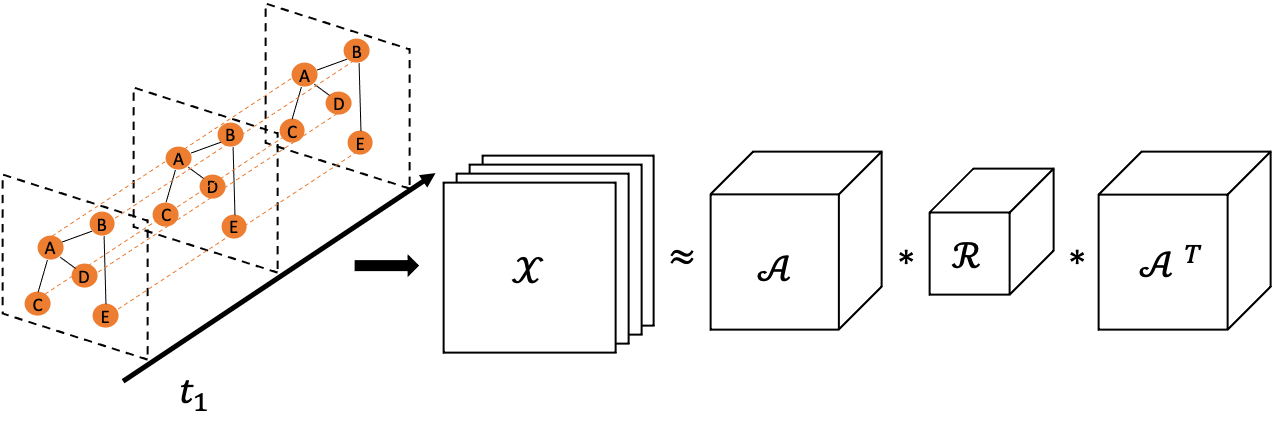
Figure 1. Algorithm Overview

3.1. Problem Formulation

Given a temporal network consisting of a sequence of network snapshots $\bm{\mathscr{G}}=\{\bm{\mathscr{G}}_{1},\dots,\bm{\mathscr{G}}_{T}\}$, we construct a temporal adjacency tensor $\bm{\mathscr{X}}:\mathbb{R}^{n\times n\times T}$, each of the frontal slice of the tensor $\bm{\mathscr{X}}(:,:,t)$ is set to the adjacency matrix of the network snapshot at timestamp $t=\{1,\dots,T\}$ (Fig. 1). In this way, we extend the modeling of the network structure to a three-way tensor with the temporal evolution explicitly spanned and accommodated along the third dimension. Our key intuition is that the decomposition structure of RESCAL, especially its request of a single matrix $A$ to be shared by all timestamps, is not sufficient to fully capture the fruitful temporally evolving information. In contrast, we introduce $T$ matrices and collect them into the $n\times r\times T$ tensor $\bm{\mathscr{A}}$, so that each of the frontal slice $\bm{\mathscr{A}}(:,:,t)$ models the latent representation of each node at time $t$. In addition, we propose to capture the cross-slice intercorrelation among the T matrices of $\bm{\mathscr{A}}$, together with the same $r\times r\times T$ tensor $\bm{\mathscr{R}}$ as RESCAL, by the circular convolution-based t-product. As a result, we formulate the objective function of Toffee  as follows,

(3) $$\arg\min_{\bm{\mathscr{A}},\bm{\mathscr{R}}}\frac{1}{2}\|\bm{\mathscr{X}}-\bm{\mathscr{A}}*\bm{\mathscr{R}}*\bm{\mathscr{A}}^{\top}\|_{F}^{2}+\frac{\lambda_{A}}{2}\|\bm{\mathscr{A}}\|_{F}^{2}+\frac{\lambda_{R}}{2}\|\bm{\mathscr{R}}\|_{F}^{2},$$

where the regularizations with parameters $\lambda_{A}$ and $\lambda_{R}$ are introduced on $\bm{\mathscr{A}}$ and $\bm{\mathscr{R}}$ to prevent overfitting. Toffee  can also support other regularizations but we omit more complicated choices for illustrative purposes.

The optimization of the Toffee  model takes advantage of the well-known relationship between the convolution operation and the Fourier transformation (Kolba and Parks, 1977; Kilmer et al., 2013), which converts the problem to Fourier domain and is parallelizable among $T$ slices. In detail, we first transform the temporal tensor $\bm{\mathscr{X}}$ to the Fourier domain along the temporal mode by $\bm{\mathscr{X}}_{\mathscr{F}}={\tt fft}(\bm{\mathscr{X}},[\hskip 2.84526pt],3)$, and then perform the rank-$r$ factorization on the block diagonal matrix $X_{\mathscr{F}}:={\tt blockdiag}(\bm{\mathscr{X}}_{\mathscr{F}})$ into the block diagonal matrices of $\bm{\mathscr{A}}$ and $\bm{\mathscr{R}}$. This can be further decomposed into $T$ independent optimization problems by decomposing each block of the diagonal $X_{\mathscr{F}}^{(k)}$ with the $k\in[t]$-th being,

$$\begin{split}\arg\min_{A_{\mathscr{F}}^{(k)},R_{\mathscr{F}}^{(k)}}&\frac{1}{2T}\|X_{\mathscr{F}}^{(k)}-A_{\mathscr{F}}^{(k)}\cdot R_{\mathscr{F}}^{(k)}\cdot(A_{\mathscr{F}}^{(k)})^{\top}\|_{F}^{2}\\ &+\frac{\lambda_{A}}{2T}\|A_{\mathscr{F}}^{(k)}\|_{F}^{2}+\frac{\lambda_{R}}{2T}\|R_{\mathscr{F}}^{(k)}\|_{F}^{2},\end{split}$$

where $\cdot$ denotes the matrix multiplication, $A_{\mathscr{F}}^{(k)}$ and $R_{\mathscr{F}}^{(k)}$ can be seen as each block of the block diagonal matrices $A_{\mathscr{F}}$ and $R_{\mathscr{F}}$. We then optimize them alternatively for each of the $T$-blocks in parallel.

3.2. Optimization

Update $A_{\mathscr{F}}^{(k)}$. To derive the update rule of $A_{\mathscr{F}}^{(k)}$, we extend the ASALSAN algorithm (Bader et al., 2007) to Fourier domain, where we first fix $R_{\mathscr{F}}^{(k)}$ and convert the objective function regarding $A_{\mathscr{F}}^{(k)}$ as

$$\arg\min_{A_{\mathscr{F}}^{(k)}}\frac{1}{2r}\|\hbox to0.0pt{\hskip 3.22624pt\leavevmode\hbox{\set@color$\overline{\hbox{}}$}\hss}{\leavevmode\hbox{\set@color$X_{\mathscr{F}}^{(k)}$}}-A_{\mathscr{F}}^{(k)}\cdot\hbox to0.0pt{\hskip 2.59656pt\leavevmode\hbox{\set@color$\overline{\hbox{}}$}\hss}{\leavevmode\hbox{\set@color$R_{\mathscr{F}}^{(k)}$}}\cdot\left(I\otimes(\hbox to0.0pt{\hskip 4.27pt\leavevmode\hbox{\set@color$\overline{\hbox{}}$}\hss}{\leavevmode\hbox{\set@color$A_{\mathscr{F}}^{(k)})$}}^{\top}\right)\|_{F}^{2}+\frac{\lambda_{A}}{2r}(\|A_{\mathscr{F}}^{(k)}\|_{F}^{2}),$$

where  $\overline{\hbox{}}$$X_{\mathscr{F}}^{(k)}$,  $\overline{\hbox{}}$$R_{\mathscr{F}}^{(k)}$ and  $\overline{\hbox{}}$$A_{\mathscr{F}}^{(k)}$ denote $[X_{\mathscr{F}}^{(k)}~{}~{}(X_{\mathscr{F}}^{(k)})^{\top}]$, $[R_{\mathscr{F}}^{(k)}~{}~{}(R_{\mathscr{F}}^{(k)})^{\top}]$ and the right $A_{\mathscr{F}}^{(k)}$, respectively, $I$ is the identity matrix with size $n\times n$, and $\otimes$ denotes the kronecker product. We optimize the above objective function by keeping  $\overline{\hbox{}}$$A_{\mathscr{F}}^{(k)}$ as constant, and update only the left $A_{\mathscr{F}}^{(k)}$. Taking the derivative with respect to $A_{\mathscr{F}}^{(k)}$, we get the following closed-form solution

$$\begin{split}A_{\mathscr{F}}^{(k)}=&\Big{(}X_{\mathscr{F}}^{(k)}A_{\mathscr{F}}^{(k)}(R_{\mathscr{F}}^{(k)})^{\top}+(X_{\mathscr{F}}^{(k)})^{\top}A_{\mathscr{F}}^{(k)}R_{\mathscr{F}}^{(k)}\Big{)}\\ &\cdot\Big{(}R_{\mathscr{F}}^{(k)}(A_{\mathscr{F}}^{(k)})^{\top}A_{\mathscr{F}}^{(k)}(R_{\mathscr{F}}^{(k)})^{\top}+(R_{\mathscr{F}}^{(k)})^{\top}(A_{\mathscr{F}}^{(k)})^{\top}A_{\mathscr{F}}^{(k)}R_{\mathscr{F}}^{(k)}+\lambda_{A}I\Big{)}^{-1}.\end{split}$$

Update $R_{\mathscr{F}}^{(k)}$. The objective function after fixing $A_{\mathscr{F}}^{(k)}$ and vectorizing $X_{\mathscr{F}}^{(k)}$ and $R_{\mathscr{F}}^{(k)}$ is as follows

$$\arg\min_{R_{\mathscr{F}}^{(k)}}\frac{1}{2r}\|{\tt vec}(X_{\mathscr{F}}^{(k)})-(A_{\mathscr{F}}^{(k)}\otimes A_{\mathscr{F}}^{(k)})\cdot{\tt vec}(R_{\mathscr{F}}^{(k)})\|_{F}^{2}+\frac{\lambda_{R}}{2r}(\|{\tt vec}(R_{\mathscr{F}}^{(k)})\|_{2}^{2}).$$

Taking the derivative with respect to ${\tt vec}(R_{\mathscr{F}}^{(k)})$ and setting it to zero, we obtain the update for $R_{\mathscr{F}}^{(k)}$ as follows

$$\begin{split}R_{\mathscr{F}}^{(k)}=&((A_{\mathscr{F}}^{(k)}\otimes A_{\mathscr{F}}^{(k)})^{\top}(A_{\mathscr{F}}^{(k)}\otimes A_{\mathscr{F}}^{(k)})+\lambda_{R}I)^{-1}\\ &\cdot(A_{\mathscr{F}}^{(k)}\otimes A_{\mathscr{F}}^{(k)})\cdot{\tt vec}(X_{\mathscr{F}}^{(k)}).\end{split}$$

$A_{\mathscr{F}}^{(k)}$ and $R_{\mathscr{F}}^{(k)}$ are alternatively optimized until the objective converges. We then reconstruct the resulting tensor $\bm{\mathscr{A}},\bm{\mathscr{R}}$ by converting the block diagonal matrices back to the temporal domain using the inverse fft: $\bm{\mathscr{A}}={\tt ifft}(\bm{\mathscr{A}}_{\mathscr{F}},[~{}],3)$, $\bm{\mathscr{R}}={\tt ifft}(\bm{\mathscr{R}}_{\mathscr{F}},[~{}],3)$.

Embedding Design. Equipped with the factorization output, we consider the design of the embedding, i.e., compose a unique embedding for each node consisting all the temporal information. Our intuition is that such embedding should involve as much cross-timestamp interrelation as possible through the t-product as $\bm{\mathscr{A}}(i,:,:)*\bm{\mathscr{R}}$, where $\bm{\mathscr{A}}(i,:,:)$ involves the factorized temporal information of all time for node $i$. This yields a tensor of size $1\times r\times T$, which can be squeezed into an $r\times T$ matrix. We then generate the final embedding through summing along the temporal mode ($2$-nd mode) to get an $r$-dimension vector embedding for node $i$:

(4) $$\mathbf{emb_{i}}=\sum_{t=1}^{T}{\tt squeeze}(\bm{\mathscr{A}}(i,:,:)*\bm{\mathscr{R}}).$$

3.3. Complexity Analysis

For a temporal adjacency tensor $\bm{\mathscr{X}}:\mathbb{R}^{n\times n\times T}$, FFT and inverse FFT operations takes $O(N^{2}T\log(T))$ for each iteration. The computational cost of $T$ $n\times n$ matrices is dominated by the computation of $R_{\mathscr{F}}^{(k)}(A_{\mathscr{F}}^{(k)})^{\top}A_{\mathscr{F}}^{(k)}(R_{\mathscr{F}}^{(k)})^{\top}$ and $(R_{\mathscr{F}}^{(k)})^{\top}(A_{\mathscr{F}}^{(k)})^{\top}A_{\mathscr{F}}^{(k)}R_{\mathscr{F}}^{(k)}$ which has the complexity of $O(2(2r^{2}N+r^{3}))$, where $r$ is the rank and is usually a small value. The total computational complexity is summarized as $O(N^{2}T\log(T))+O(2T(2r^{2}N+r^{3}))$. The FFT operation requires forming the tensor $\bm{\mathscr{X}}$ and the output tensors $\bm{\mathscr{A}}$ and $\bm{\mathscr{R}}$, which has the storage complexity of $O(n^{2}T+nrT+r^{2}T)$.

4. Experiments

Similar to (Nguyen et al., 2018), we evaluate the network embedding generated by Toffee with the link prediction task. In the experiments, we answer two important questions:

RQ1: How does Toffee compare with other state-of-the-art temporal network embedding algorithms?

RQ2: Does the key design in Toffee help in achieving better performance?

Dataset	# Nodes	# Edges	$\bar{d}$	Timespan
fb-forum	899	34K	74	166
email-Eu-core	986	26K	25.44	526
ia-primary-school-proximity	242	126K	1K	3100
ia-contacts-hypertext2009	113	21K	368	4
ia-workplace-contacts	92	10K	213	7104
aves-wildbird-network	202	11.9K	117	2884

Table 1. Dataset Statistics

Dataset	HTNE	CTDNE	HNIP	TNE	t-SVD	RESCAL	Toffee-	Toffee
fb-forum	0.8615	0.8567	0.8091	0.6493	0.8885	0.8010	0.9280	0.9420
email-Eu-core	0.8737	0.8320	0.8312	0.6615	0.8684	0.8812	0.8912	0.9010
ia-primary-school-proximity	0.7957	0.7806	0.7957	0.6043	0.8213	0.8102	0.8162	0.8218
ia-contacts-hypertext2009	0.6956	0.5831	0.5832	0.6526	0.7669	0.7788	0.7687	0.9661
ia-workplace-contacts	0.7834	0.6653	0.7834	0.6082	0.7835	0.7146	0.7913	0.8366
aves-wildbird-network	0.8869	0.8901	0.8066	0.7018	0.9778	0.9202	0.9851	0.9936

Table 2. Link Prediction Results (Micro-F1). The best scores for each operators on each dataset are underlined, the best-performance operator algorithm is in bold.

4.1. Baselines

We compare Toffee with the following state-of-the-art temporal network embedding baselines

• TNE (Zhu et al., 2016). A matrix factorization-based temporal network embedding algorithm that jointly factorizes the temporal adjacency matrices with a uniqueness penalty term on the embeddings.

• CTDNE (Nguyen et al., 2018). A temporal network embedding algorithm that exploits the time-constrained temporal random walk using an extension to the node2vec (Grover and Leskovec, 2016) algorithm via the skip-gram model.

• HNIP (Qiu et al., 2020). A temporal network embedding algorithm that employs the high-order non-linear information as an extension to the auto-encoder-based network embedding algorithms.

• HTNE (Zuo et al., 2018). A temporal network embedding algorithm that uses a Hawkes process to capture the influence of the historical neighbors on the current neighbor.

To investigate the benefits of the key components, we also compare our proposed Toffee with RESCAL (Nickel et al., 2011) and t-SVD (Kilmer and Martin, 2011; Zhang et al., 2014) which differs from Toffee in that RESCAL uses a single matrix as representation of each entity (node), and t-SVD solves the truncated SVD in the Fourier domain, which will result in an f-diagonal middle tensor $\bm{\mathscr{S}}$. We also compare with Toffee^-, which is Toffee without regularizations.

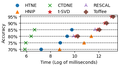
Figure 2. The time it takes for each method to reach different levels of accuracy for aves-wildbird-network dataset.

4.2. Experiment Setup

Experiments are conducted on six temporal network datasets from the Network Repository (Rossi and Ahmed, 2015) which are densely connected (with high average degrees $\bar{d}$) to verify the effectiveness of Toffee in capturing global structure information. The statistics of the temporal networks are summarized in Table 1.

The regularization parameters $\lambda_{A}$ and $\lambda_{R}$ in Toffee is determined through grid-search among $\{1^{-4},1^{-3},1^{-2},1^{-1}\}$. To fairly compare with RESCAL and t-SVD, we use the same embedding construction method as Toffee in eq.(4) to encode sufficient temporal information (for RESCAL we use matrix product instead of t-product). For CTDNE, HNIP, and HTNE, we adopt the same hyper-parameter settings as in paper (Qiu et al., 2020). For TNE, we take the embeddings of last timestamp for evaluations. For all the tested algorithms, the embedding dimension is set to 128 (ia-contacts-hypertext2009 and ia-workplace-contacts have embedding dimension as 64 since the number of nodes are less than 128).

For the link prediction task, we adopt the same experiment settings as in (Nguyen et al., 2018) that we select the first 75% of the temporal links for learning the embeddings, and train a logistic regression classifier on the rest 25% of the temporal links as positive examples, combined with the same number of negative examples generated by random sampling from the non-existing links. The links between two nodes are defined as edge representations and are calculated with four different operators defined in (Grover and Leskovec, 2016). We report the average Micro-F1 score of 10 replications based on 10 different seeds of initializations.

4.3. Link Prediction

Similar to (Nguyen et al., 2018; Qiu et al., 2018; Zuo et al., 2018), we evaluate the effectiveness of the Toffee extracted embeddings on the link prediction task. The aim of link prediction task is to determine whether there will be an edge between two nodes in the future based on the embeddings learned from the past to measure the prediction ability of the embeddings.

Table 2 shows the Micro-F1 score for the link prediction task with edge representation computed by multiple operators. First of all, results demonstrate that Toffee significantly outperforms other baselines considering the best-performance operator (RQ1). This is due to the fact that Toffee can better exploit the global network structure compared with the baselines which infer the network embeddings based on neighborhood information. Specifically, all tensor based algorithms including t-SVD, RESCAL, and Toffee have better performance compared with the neighborhood-based algorithms CTDNE, HNIP, and HTNE considering the best-achievable operator, which also verifies that tensor based methods can better capture the global structure information. Those tensor-based methods also beat the matrix-based method TNE, indicating the superiority of tensors in jointly modeling the temporal and structural information between nodes. In addition, it is also worth noticing that even with no regularizations on tensor $\bm{\mathscr{A}}$ and $\bm{\mathscr{R}}$, Toffee^- can outperform the baselines. This means that Toffee can help reducing the effort of hyper-parameter tuning.

Fig. 2 shows that Toffee achieves significantly better accuracy with more time cost compared with HTNE, HNIP, CTDNE – illustrating that in order to get more accurate network representations, we have to sacrifice some time cost. However, compared with tensor-based methods, t-SVD and RESCAL, which offer superior performance than HTNE, HNIP, CTDNE, Toffee is able to achieve better accuracy with little trade-off in terms of computational cost.

Furthermore, we observe that Toffee outperforms both t-SVD and RESCAL (RQ2). The performance gain over RESCAL verifies that Toffee benefits from the tensor product which will help better capture the temporal correlation by the circular convolution operator. Notice that without regularization, Toffee^- resembles the results of t-SVD with slight higher accuracy. This is because each slice in tensor $\bm{\mathscr{R}}$ is able to capture the directional information between the latent groups of each node, which is not efficiently encoded in the results of t-SVD with information concentrated only on the diagonals. In addition to this, Toffee largely outperforms t-SVD thanks to the regularization terms on tensors $\bm{\mathscr{A}}$ and $\bm{\mathscr{R}}$.

5. Conclusion

In this paper, we have proposed Toffee, an advanced tensor decomposition algorithm for temporal network embedding. The exploitation of t-product enables Toffee to better capture the cross-time information among different temporal slices of the temporal network. We demonstrate the effectiveness of Toffee with the temporal link prediction task with multiple real-world datasets. Experiment results show significant improvement over state-of-the-art temporal network embedding algorithms. Future works include involving the attribute information and further demonstrating the effectiveness of Toffee on other downstreaming tasks.

- (1)
- Bader et al. (2007) Brett W Bader, Richard A Harshman, and Tamara G Kolda. 2007. Temporal analysis of semantic graphs using ASALSAN. In Seventh IEEE ICDM 2007. IEEE, 33–42.
- Cao et al. (2015) Shaosheng Cao, Wei Lu, and Qiongkai Xu. 2015. Grarep: Learning graph representations with global structural information. In Proc. of the 24th ACM CIKM. ACM, 891–900.
- Gauvin et al. (2014) Laetitia Gauvin, André Panisson, and Ciro Cattuto. 2014. Detecting the community structure and activity patterns of temporal networks: a non-negative tensor factorization approach. PloS one 9, 1 (2014), e86028.
- Grover and Leskovec (2016) Aditya Grover and Jure Leskovec. 2016. node2vec: Scalable feature learning for networks. In Proc. of the 22nd ACM SIGKDD. ACM, 855–864.
- Kilmer et al. (2013) Misha E Kilmer, Karen Braman, Ning Hao, and Randy C Hoover. 2013. Third-order tensors as operators on matrices: A theoretical and computational framework with applications in imaging. SIAM J. Matrix Anal. Appl. 34, 1 (2013), 148–172.
- Kilmer and Martin (2011) Misha E Kilmer and Carla D Martin. 2011. Factorization strategies for third-order tensors. Linear Algebra Appl. 435, 3 (2011), 641–658.
- Kolba and Parks (1977) D Kolba and TW Parks. 1977. A prime factor FFT algorithm using high-speed convolution. IEEE Transactions on Acoustics, Speech, and Signal Processing 25, 4 (1977), 281–294.
- Nguyen et al. (2018) Giang Hoang Nguyen, John Boaz Lee, Ryan A Rossi, Nesreen K Ahmed, Eunyee Koh, and Sungchul Kim. 2018. Continuous-time dynamic network embeddings. In Companion Proc. of WWW 2018. International World Wide Web Conferences Steering Committee, 969–976.
- Nickel et al. (2011) Maximilian Nickel, Volker Tresp, and Hans-Peter Kriegel. 2011. A Three-Way Model for Collective Learning on Multi-Relational Data.
- Perozzi et al. (2014) Bryan Perozzi, Rami Al-Rfou, and Steven Skiena. 2014. Deepwalk: Online learning of social representations. In Proc. of the 20th ACM SIGKDD. ACM, 701–710.
- Qiu et al. (2018) Jiezhong Qiu, Yuxiao Dong, Hao Ma, Jian Li, Kuansan Wang, and Jie Tang. 2018. Network embedding as matrix factorization: Unifying deepwalk, line, pte, and node2vec. In Proc. of the 11th ACM WSDM. ACM, 459–467.
- Qiu et al. (2020) Zhenyu Qiu, Wenbin Hu, Jia Wu, Weiwei Liu, Bo Du, and Xiaohua Jia. 2020. Temporal Network Embedding with High-Order Nonlinear Information.. In AAAI. 5436–5443.
- Rader (1968) Charles M Rader. 1968. Discrete Fourier transforms when the number of data samples is prime. Proc. IEEE 56, 6 (1968), 1107–1108.
- Rossi and Ahmed (2015) Ryan A. Rossi and Nesreen K. Ahmed. 2015. The Network Data Repository with Interactive Graph Analytics and Visualization. In AAAI. http://networkrepository.com
- Tang et al. (2015) Jian Tang, Meng Qu, Mingzhe Wang, Ming Zhang, Jun Yan, and Qiaozhu Mei. 2015. Line: Large-scale information network embedding. In Proc. of the 24th WWW. International World Wide Web Conferences Steering Committee, 1067–1077.
- Zhang et al. (2014) Zemin Zhang, Gregory Ely, Shuchin Aeron, Ning Hao, and Misha Kilmer. 2014. Novel methods for multilinear data completion and de-noising based on tensor-SVD. In Proc. of the IEEE CVPR. 3842–3849.
- Zhu et al. (2016) Linhong Zhu, Dong Guo, Junming Yin, Greg Ver Steeg, and Aram Galstyan. 2016. Scalable temporal latent space inference for link prediction in dynamic social networks. IEEE TKDE 28, 10 (2016), 2765–2777.
- Zuo et al. (2018) Yuan Zuo, Guannan Liu, Hao Lin, Jia Guo, Xiaoqian Hu, and Junjie Wu. 2018. Embedding temporal network via neighborhood formation. In Proc. of the 24th ACM SIGKDD. ACM, 2857–2866.