A puzzle solved after two decades: SN 2002gh among the brightest of superluminous supernovae

Abstract

We present optical photometry and spectroscopy of the superluminous SN 2002gh from maximum light to $+204$ days, obtained as part of the Carnegie Type II Supernova (CATS) project. SN 2002gh is among the most luminous discovered supernovae ever, yet it remained unnoticed for nearly two decades. Using Dark Energy Camera archival images we identify the potential SN host galaxy as a faint dwarf galaxy, presumably having low metallicity, and in an apparent merging process with other nearby dwarf galaxies. We show that SN 2002gh is among the brightest hydrogen-poor SLSNe with $M_{V}=-22.40\pm 0.02$, with an estimated peak bolometric luminosity of $2.6\pm 0.1\times 10^{44}$ erg s^-1. We discount the decay of radioactive nickel as the main SN power mechanism, and assuming that the SN is powered by the spin down of a magnetar we obtain two alternative solutions. The first case, is characterized by significant magnetar power leakage, and $M_{\mathrm{ej}}$ between 0.6 and 3.2 $M_{\sun}$, $P_{\mathrm{spin}}=3.2$ ms, and $B=5\times 10^{13}$ G. The second case does not require power leakage, resulting in a huge ejecta mass of about 30 $M_{\sun}$, a fast spin period of $P_{\mathrm{spin}}\sim 1$ ms, and $B\sim 1.6\times 10^{14}$ G. We estimate a zero-age main-sequence mass between 14 and 25 $M_{\sun}$ for the first case and of about 135 $M_{\sun}$ for the second case. The latter case would place the SN progenitor among the most massive stars observed to explode as a SN.

1 Introduction

The first half of the 21^st century will be remembered as a revolutionary epoch for time-domain astronomy. Thanks to large area and untargeted transient surveys, astronomers are exploring the time-domain Universe to an unprecedented level, discovering transient events that span a wide range of timescales and luminosities. One of the most spectacular such transients are the rare class of supernovae (SNe) initially characterized by their extremely bright peak luminosities ($\simeq-21$ mag at optical wavelengths) powered by a non-standard source of energy, that have challenged our understanding of massive star evolution and explosion.

These rare and bright SNe are commonly referred to as superluminous SNe (SLSNe). Like their lower luminosity cousins they are divided into subtypes based on the presence of hydrogen in their spectra as hydrogen-rich (Type II) and hydrogren-poor (Type I) (see Moriya et al., 2018; Gal-Yam, 2019a). Some SLSNe-II show relatively narrow hydrogen emission lines on top of a broad component, characteristic of SNe Type IIn (see Schlegel, 1990), and evidence of interaction between the energetic SN ejecta and a massive hydrogen-rich circum-stellar medium (CSM), such as SN 2006gy (Smith et al., 2007; Ofek et al., 2007). These SLSNe-II are usually considered the bright end of Type IIn SNe, although it is unclear whether an additional power source other than the strong ejecta-CSM interaction and radioactive decay significantly contributes to their extreme luminosities (see e.g., Woosley et al., 2007; Jerkstrand et al., 2020). The idea of an additional power source is reinforced by some SLSNe-II that do not show clear signatures of strong ejecta-CSM interaction (Gezari et al., 2009; Miller et al., 2009; Inserra et al., 2018; Dessart, 2018). A potential power source is the energy injection from the spin down of a fast rotating neutron star with an extremely powerful magnetic field, a magnetar, as explained below. Other notable events of the SLSN class, are a handful of objects initially classified as hydrogen-poor SLSNe, but several days after maximum light reveal hydrogen features and signatures of ejecta-CSM interaction (Yan et al., 2015, 2017), suggesting that some hydrogen-poor SLSNe lose their hydrogen envelopes shortly before their final explosion.

Objects such as SN 1999as (Knop et al., 1999), SN 2005ap (Quimby et al., 2007), SCP 06F6 (Barbary et al., 2009), and SN 2007bi (Gal-Yam et al., 2009) were the first SLSN-I reported, several years before they were distinguished as a separate SN class. Their bright peak luminosities together with the identification of a common set of spectral features made it possible to distinguish them as members of a completely new SN class (Quimby et al., 2011). These SLSNe are characterized by their extreme peak luminosities, very blue and nearly featureless optical spectral emission, the lack of hydrogen and helium lines and the presence of O ii and C ii absorption lines before and close to maximum light (Quimby et al., 2011). A few weeks after maximum light, when the ejecta are cool enough, SLSN-I spectra become similar to SNe Ic (e.g., Pastorello et al., 2010) or to broad line SNe Ic (SNe Ic-BL; Liu et al., 2017) at an early phase. Their nebular spectra also show some similarity with the nebular spectra of SNe Ic-BL (Milisavljevic et al., 2013; Jerkstrand et al., 2017; Nicholl et al., 2016b; Nicholl et al., 2019).

One of the first models proposed to account for the large luminosity displayed by SLSNe was the radioactive decay of several solar masses of ⁵⁶Ni (Quimby et al., 2007; Gal-Yam et al., 2009), synthesized in a Pair Instability SN (PISN) (Barkat et al., 1967; Rakavy & Shaviv, 1967). PISNe are the theoretical explosions of low metallicity and very massive main-sequence stars ($\sim 140-260$ M_☉), ejecting several tens of solar masses of ⁵⁶Ni (Heger & Woosley, 2002). These objects are expected to be common in the early Universe. The large amount of radioactive material ejected by PISNe can potentially power the extreme luminosities observed in SLSNe, however, some hydrogen-poor SLSNe fade too fast after peak to be consistent with the ⁵⁶Ni $\rightarrow$ ⁵⁶Co $\rightarrow$ ⁵⁶Fe decay chain, arguing against this power mechanism. Also the large opacity of iron-peak elements is expected to shift the emission towards near-infrared wavelengths (NIR), which is in conflict with the very blue continuum displayed by hydrogen-poor SLSNe (Dessart et al., 2012). Additional evidence against hydrogen-poor SLSNe being the result of PISNe, comes from the comparison between the observed spectra of SLSNe at nebular phases, which are dominated by emission lines of intermediate mass elements (Milisavljevic et al., 2013; Jerkstrand et al., 2017; Nicholl et al., 2016b; Nicholl et al., 2019; Mazzali et al., 2019), in contrast with the iron-peak element dominated nebular emission predicted for PISNe (see e.g., Dessart et al., 2012; Jerkstrand et al., 2016; Mazzali et al., 2019).

An alternative model to explain the light curve evolution of hydrogen-poor SLSNe invokes the spin-down of a highly magnetic newborn neutron star, a “magnetar”, that energises the SN ejecta (Maeda et al., 2007; Woosley, 2010; Kasen & Bildsten, 2010). The magnetar model was introduced by Maeda et al. (2007) to explain the peculiar double peaked and fast declining light curve of the Type Ib SN 2005bf. After the recognition of SLSNe as a new class, and using a small sample of well observed hydrogen-poor SLSNe, Inserra et al. (2013) fitted an analytic magnetar model to their sample bolometric light curves and first showed that the power injection from the spin down of a magnetar can successfully reproduce the complete light curve evolution, including a light curve flattening at late times ($\sim 200$ days), that cannot be explained by the ⁵⁶Co radioactive decay. More recently, Nicholl et al. (2017) presented a more sophisticaded version of the magnetar model built-in the Modular Open Source Fitter for Transients (MOSFiT; Guillochon et al., 2018). They applied their magnetar model to a large sample of hydrogen-poor SLSNe collected from the literature and showed that such a magnetar model can explain the light curve evolution of many objects of this class. Another alternative mechanism to power SLSN-I luminosity, is the SN ejecta-CSM interaction with a hydrogen and helium free CSM. For complete recent reviews on the SLSNe properties and their power sources see Gal-Yam (2019a) and Moriya et al. (2018).

Recently, the light curves of the hydrogen-poor SLSNe discovered in the course of the Palomar Transient Factory (PTF; De Cia et al., 2018), the Pan-STARRS1 Medium Deep Survey (PS1; Lunnan et al., 2018) and the Dark Energy Survey (DES; Angus et al., 2019) were presented and analysed. These surveys show that the low-luminosity tail of the SLSN population extends and overlaps in luminosity with the normal stripped envelope core collapse SN (CCSN) population. Although there is a continuous distribution in brightness from SNe Ic, Ic-BL to SLSNe-I, and rare examples of non-SLSNe powered by a magnetar exist (e.g., Maeda et al., 2007; Grayling et al., 2021), the dominant power mechanism seems to be different in the different SN populations. The well-sampled multi-band light curves provided by these surveys, confirmed the large diversity in the morphology of SLSN light curves, many of them showing bumps in their light curve evolution (see e.g., Nicholl et al., 2015; Smith et al., 2016; Yan et al., 2017).

The host galaxies of hydrogen-poor SLSNe are characterized by being low mass dwarf galaxies ($M_{\mathrm{stellar}}<2\times 10^{9}\mathrm{M}_{\sun}$; e.g., Neill et al., 2011; Lunnan et al., 2014; Leloudas et al., 2015; Angus et al., 2016; Perley et al., 2016; Schulze et al., 2018), usually of irregular morphology with roughly half of the galaxies exhibiting a morphology that is either asymmetric, off-centre or consisting of multiple peaks (Lunnan et al., 2015), the latter being a possible signature of merging systems. SLSN host galaxies are clearly different from the galaxies hosting normal core-collapse SNe (CCSNe), which are more massive and in general exhibit spiral structure. SLSN-I host galaxies are also characterized by low metallicities ($Z\leq 0.5Z_{\sun}$; e.g., Lunnan et al., 2014; Leloudas et al., 2015; Perley et al., 2016; Schulze et al., 2018), and by high specific Star Formation Rates (sSFR $\sim 10^{-9}$ yr^-1; e.g., Neill et al., 2011; Lunnan et al., 2014; Perley et al., 2016). The host galaxies of SLSNe-II are more diverse, showing a range of properties varing from low mass and metal poor dwarf galaxies, similar to the hosts of hydrogen-poor objects, to bright spiral galaxies similar to the hosts of normal CCSNe (Leloudas et al., 2015; Perley et al., 2016; Schulze et al., 2018).

Here we present and analyse observations of SN 2002gh obtained by the “Carnegie Type II Supernova Survey” (CATS, hereafter). CATS was a SN follow-up program similar to its successor the Carnegie Supernova Program (CSP; Hamuy et al., 2006), carried out at Las Campanas Observatory during 2002–2003 with the main purpose to study nearby ($z<0.05$) SNe II. In the course of the CATS survey we included a handful of SNe of other classes. More details about the CATS program and the instruments used can be found in Hamuy et al. (2006, 2009) and Cartier et al. (2014). Remarkably, CATS results include observations of SN 2002ic, the first SN Ia showing interaction with a dense circumstellar medium (Hamuy et al., 2003), and SN 2003bg the first Type IIb hypernova (Hamuy et al., 2009). Here we add to these notable achievements, the observations of SN 2002gh, the second SLSN discovered after SN 1999as (Knop et al., 1999), for which its superluminous nature remained unnoticed for nearly two decades until now. In Section 2 we describe the data reduction and present the observations. In Section 3.1, we identify the defining SLSN-I spectral features in the spectra of SN 2002gh by comparing with other well studied objects, and measure line velocities. In Section 3.2 we use Dark Energy Camera (Flaugher et al., 2015) archival images to identify and characterize the potential SN host galaxy. In Section 3.3 we characterize the light curves of SN 2002gh and in Section 3.4 we use blackbody fits to estimate the bolometric peak luminosity and the total radiated energy. We compare the bolometric light curve of SN 2002gh with SLSNe from the PS1 and DES surveys, showing that SN 2002gh is among the brightest hydrogen-poor SLSNe. In Section 3.5 we explore the magnetar model and the radioactive decay of ⁵⁶Ni as potential power sources to explain the extreme luminosity of SN 2002gh, and discuss potential signatures of ejecta-CSM interaction. Throughout this paper we adopt a $\Lambda$CDM cosmology with Hubble constant $H_{0}=70$ km s^-1 Mpc^-1, total dark matter density $\Omega_{M}=0.3$ and dark energy density $\Omega_{\Lambda}=0.7$ in our calculations. Finally, in Section 4 we discuss and summarize our results.

2 Observations and Data Reduction

SN 2002gh was discovered by the Nearby Supernova Factory (Aldering et al., 2002) on 2002 October 5 (MJD=52552.41) at an unfiltered magnitude of 19.3 (Wood-Vasey et al., 2002). Previous to the SN discovery, a non-detection on 2001 December 14 reported by Wood-Vasey et al. (2002) places a 5$\sigma$ upper limit on the SN magnitude of 21.2 mag. The Nearby Supernova Factory photometry of SN 2002gh was calibrated to the USNO A1.0 “red” catalog, and therefore is similar to $R$-band photometry (Wood-Vasey, private communication).

The SN was located at $\alpha$=03:05:29.46 $\delta$=$-$05:21:56.99 (J2000.0). No host galaxy was clearly associated with SN 2002gh in the CATS images to the limiting magnitude of the deepest CATS images. The limiting magnitude of CATS images are $\sim 23$ mag in $BV$ and $\sim 21.5$ mag in $I$ band, this is 0.5 to 1 mag fainter than the faintest detection of SN 2002gh. A nearby galaxy at 8$\aas@@fstack{\prime\prime}$6 west and 6$\aas@@fstack{\prime\prime}$2 south from the SN and at $z=0.133$, indicated as G1 in Fig. 1, was originally identified as the possible host. However, after inspecting our highest signal-to-noise ratio ($S/N$) spectra, we detected Mg ii $\lambda\lambda$ $2796,2803$ doublet narrow absorption lines from the host galaxy. We model the Mg ii $\lambda\lambda$ $2796,2803$ doublet in these good $S/N$ spectra by fitting simultaneously two Gaussian profiles (see Fig. 2), where the relative central wavelengths are fixed accordingly and the variance of the Gaussian profiles were also fixed according to the spectral resolution of the instrument used to obtain the spectra. We adopt the median value from these four independent measurements and use three significant digits for the uncertainty. This is to take into account any unaccounted uncertainty affecting our redshift measurements, adopting $z=0.365\pm 0.001$ as the redshift for SN 2002gh. This redshift makes the SN spectra consistent with other hydrogen-poor SLSNe-I as discussed below in Section 3.1.

The data were reduced using custom IRAF scripts. A full description of the instruments characteristics and the reduction procedures can be found in Hamuy et al. (2006, 2009) and Cartier et al. (2014).

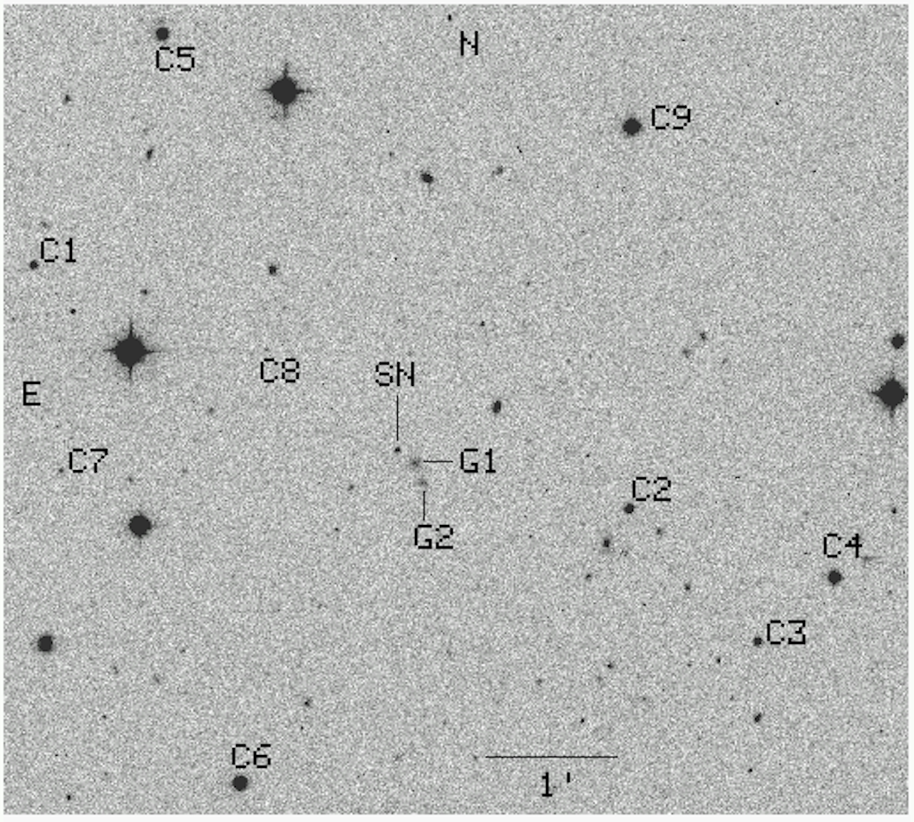
Figure 1: Field of SN 2002gh observed with the Swope 1 m telescope in the $V$-band when the SN was near maximum light. North is up and east is to the left. We label SN 2002gh along with nine comparison stars used to derive the differential photometry of the SN. Two nearby galaxies to the south-west of the SN are indicated as G1 and G2. Galaxy G1 has a redshift of 0.133 and was originally identified as the possible host. The image scale is shown with a horizontal line near the bottom.

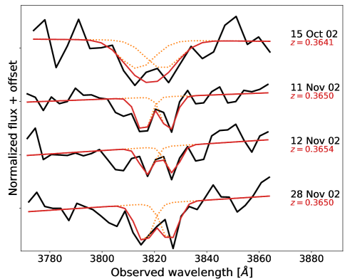
Figure 2: Spectra of SN 2002gh around the region of the Mg ii $\lambda\lambda$ $2796,2803$ doublet in the observer frame (in black), these spectra have been chosen because of their good signal-to-noise ratio in this region. The epoch of the spectra is indicated on the right and the instruments and their characteristics are listed in Table 3. The full Gaussian profile fits to the Mg ii $\lambda\lambda$ $2796,2803$ doublet are shown in red and the individual Gaussian profiles are shown as orange-dotted lines. The redshift obtained for each spectrum is given on the right, and the median redshift for SN 2002gh is $z=0.365\pm 0.001$.

2.1 Photometry

We obtained 22 epochs of $BVI$ optical photometry as part of the CATS project (Hamuy et al., 2009), beginning 10 days after the SN discovery. Our first photometric observations were obtained six days before bolometric maximum light and extend to $+204$ rest-frame days after peak. The photometry is summarized in Table 1 and the SN light curves are shown in Fig. 3. The SN photometry was calibrated differentially relative to a set of 9 stars in the field as shown in Fig. 1. This local photometric sequence was calibrated in the Vega system on photometric nights with the Swope telescope at Las Campanas Observatory. The instrumental magnitudes of the local standard stars and of the SN were converted to the standard system using the colour terms and equations of Hamuy et al. (2009). Their average $BVRI$ magnitudes are summarized in Table 2.

We interpolated the SN light curves using the python Gaussian process module implemented in scikit-learn (Pedregosa et al., 2011). We used the radial-basis funnction (RBF) kernel for well-sampled light curves, while the Matern kernel with $\nu=3/2$ was used for light curves with long gaps, such as the $V$ band, or to extrapolate the $R-$band light curve. The kernel hyperparameters were optimized by maximizing the log-marginal-likelihood (LML). As the LML may have multiple local optima, the optimizer was started 10 times. The first run was conducted starting from guess hyperparameter values. The subsequent runs were conducted from hyperparameter values that have been chosen randomly from the range of allowed values. We present our interpolated light curves in Fig. 3.

We used the interpolated light curves or the photometry from Table 1 to improve the flux calibration of the spectra presented in Section 2.2. When photomometry was obtained on the same night of a spectrum we used the observed photometry, otherwise we used the interpolated light curves. The mangling of the spectra was perfomed using a low-order polynomial to match the spectral flux to the SN photometry. The aim is to scale the flux calibration and correct any wavelength dependent slit loss, and not to significantly alter the spectra. The application of this procedure to the spectra yields a small change in the spectral shape, if any.

Then, we obtained additional photometry by computing synthetic photometry from the mangled SN spectra (see Fig. 3), thus adding relevant photometric information in the $R$ band. The sythentic photometry was computed as described in Bessell (2005), using the Johnson-Cousins $BVRI$ response functions of Bessell (1990). The difference between the synthetic photometry and the interpolated and observed photometry is always below 5%, but we conservatively quote an uncertainty of 0.15 mag for the computed synthetic photometry.

Table 1: Optical photometry of SN 2002gh

Date UT	MJD	$B$	$V$	$I$	Tel.
2002-10-15	52562.8	–	19.258($0.010$)	–	LDSS-2/Baade
2002-10-25	52572.7	–	19.198($0.022$)	19.026($0.028$)	CCD/Swope
2002-10-25	52572.8	–	19.209($0.016$)	–	LDSS-2/Baade
2002-10-27	52574.7	–	19.241($0.015$)	19.059($0.036$)	CCD/CTIO 0.9 m
2002-10-29	52576.8	19.475($0.017$)	19.281($0.014$)	–	LDSS-2/Baade
2002-10-30	52577.8	19.527($0.020$)	19.283($0.014$)	–	WFCCD/du Pont
2002-11-07	52585.8	–	19.316($0.024$)	–	WFCCD/du Pont
2002-11-07	52585.8	19.705($0.031$)	19.285($0.018$)	19.012($0.054$)	CCD/Swope
2002-11-08	52586.8	19.643($0.016$)	19.336($0.014$)	19.112($0.038$)	CCD/Swope
2002-11-12	52590.8	19.732($0.039$)	19.343($0.032$)	18.946($0.111$)	CCD/Swope
2002-11-18	52596.7	19.983($0.085$)	19.476($0.044$)	18.974($0.061$)	CCD/Swope
2002-12-03	52611.7	20.219($0.019$)	19.624($0.023$)	19.168($0.037$)	WFCCD/du Pont
2002-12-07	52615.8	20.287($0.066$)	19.651($0.055$)	–	CCD/Swope
2002-12-11	52619.6	–	–	19.253($0.026$)	CCD/Swope
2003-01-07	52646.6	20.722($0.033$)	19.963($0.020$)	19.404($0.053$)	CCD/Swope
2003-01-26	52665.6	20.908($0.037$)	20.138($0.021$)	19.459($0.035$)	CCD/Swope
2003-02-02	52672.6	–	20.286($0.024$)	19.563($0.039$)	CCD/Swope
2003-02-03	52673.6	–	20.315($0.068$)	–	WFCCD/du Pont
2003-03-03	52701.5	22.026($0.067$)	20.899($0.046$)	20.282($0.090$)	WFCCD/du Pont
2003-03-12	52710.5	–	21.159($0.097$)	20.648($0.142$)	WFCCD/du Pont
2003-07-21	52841.9	–	22.379($0.158$)	–	CCD/Swope
2003-07-28	52848.9	–	22.619($0.229$)	–	CCD/Swope

• Numbers in parentheses correspond to 1 $\sigma$ statistical uncertainties.

Table 2: $BVRI$ photometric sequence around SN 2002gh.

Star	R.A.	Dec	$B$	$V$	$R$	$I$
C1	03:05:40.66	$-$05:20:36.77	18.997(0.040)	18.104(0.013)	18.450(0.017)	17.042(0.009)
C2	03:05:22.31	$-$05:22:21.09	18.466(0.042)	17.572(0.015)	17.936(0.015)	16.529(0.009)
C3	03:05:18.29	$-$05:23:20.11	18.876(0.019)	17.799(0.025)	18.106(0.015)	16.425(0.015)
C4	03:05:16.00	$-$05:22:50.10	16.684(0.015)	15.955(0.019)	–	15.029(0.010)
C5	03:05:36.90	$-$05:18:49.67	17.067(0.037)	16.067(0.015)	16.399(0.015)	15.005(0.008)
C6	03:05:33.99	$-$05:24:30.93	16.094(0.031)	15.429(0.024)	15.987(0.015)	14.656(0.010)
C7	03:05:39.72	$-$05:22:11.62	22.764(0.538)	21.385(0.093)	21.892(0.366)	18.795(0.026)
C8	03:05:33.46	$-$05:21:12.59	22.869(0.339)	21.296(0.162)	20.873(0.146)	18.665(0.024)
C9	03:05:22.52	$-$05:19:26.92	15.590(0.031)	14.903(0.014)	15.416(0.015)	–

• Numbers in parentheses correspond to 1 $\sigma$ statistical uncertainties.

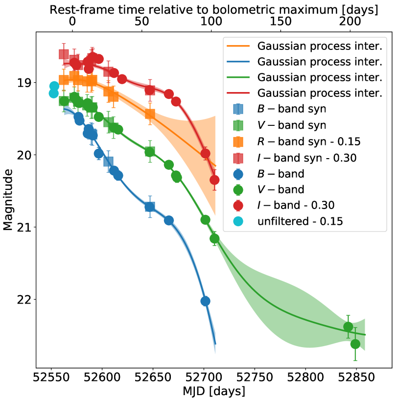
Figure 3: Optical light curves of SN 2002gh. We present $BVI$ photometry obtained in the course of the CATS project (Hamuy et al., 2009), unfiltered photometry reported by Wood-Vasey et al. (2002), and $BVRI$ synthetic photometry computed from the spectra after matching them to the interpolated photometry. The legend is presented on the top right of the figure.

2.2 Spectroscopy

A total of ten spectra of SN 2002gh were obtained, spanning from -6 to +56 rest-frame days relative to the estimated bolometric maximum. We summarize spectroscopic observations in Table 3, and the spectral sequence is presented in Fig. 4. We improved the flux calibration by using interpolated photometry (see Section 2.1) and we fitted a modified blackbody model to the spectral sequence to estimate the blackbody radius ($R_{bb}$) and temperature ($T_{bb}$). To fit the modified blackbody model we selected pseudo-continuum emission regions. For this end, we use regions of the spectra redwards of $2900$ Å (see e.g., Prajs et al., 2017) and devoid of any strong spectral features.

Table 3: Summary of Spectroscopic Observations of SN 2002gh.

Date UT	MJD	Phase	Instrument/	Wavelength	Dispersion	Resolution
		(days)	Telescope	Range (Å)	(Å/pixel)	(Å)
2002-10-15	$52562.3$	$-6.2$	LDSS-2/Baade	$3600-9000$	$4.3$	$13.5$
2002-10-25	$52572.6$	$+1.3$	LDSS-2/Baade	$3600-9000$	$4.3$	$13.5$
2002-10-29	$52576.3$	$+4.0$	LDSS-2/Baade	$3600-9000$	$4.3$	$13.5$
2002-11-07	$52585.3$	$+10.6$	WFCCD/du Pont	$3820-9330$	$3$	$6$
2002-11-11	$52589.3$	$+13.6$	B&C Spec./Baade	$3180-9315$	$3$	$6$
2002-11-12	$52590.3$	$+14.3$	B&C Spec./Baade	$3180-9315$	$3$	$6$
2002-11-28	$52606.2$	$+25.9$	B&C Spec./Baade	$3180-9312$	$3$	$6$
2002-12-03	$52611.2$	$+29.6$	WFCCD/du Pont	$3820-9330$	$3$	$6$
2003-01-03	$52642.2$	$+52.3$	Mod. Spec./du Pont	$3780-7280$	$2$	$7$
2003-01-08	$52647.1$	$+55.9$	B&C Spec./Baade	$3180-9280$	$3$	$6$

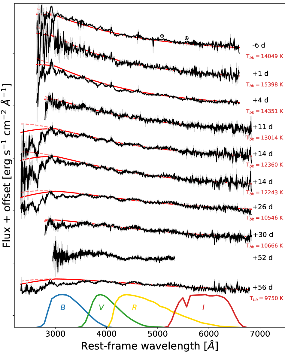
Figure 4: Spectroscopic sequence of SN 2002gh. The spectra have been mangled in order to match the $BVI$ interpolated photometry at their corresponding epoch, yielding accurate flux calibration. Then we corrected the spectra by a Galactic reddening of $E(B-V)=0.0593$ mag (Schlafly & Finkbeiner, 2011) in the line-of-sight using the Cardelli et al. (1989) reddening law with $R_{V}=3.1$. The spectra are corrected by the host galaxy redshift to place the spectra in the rest-frame system. The red solid lines correspond to modified blackbody fits to the SN spectra with a linear flux suppression below the “cutoff” wavelength at 3000 Å, and the dashed red lines correspond to the normal blackbody without flux suppression. On the right we give the phase relative to the estimated rest-frame time since bolometric maximum and the blackbody temperature ($T_{\mathrm{bb}}$). At the bottom of the figure we show the $BVRI$ normalized transmissions at the SN rest-frame.

3 Analysis

3.1 Line identification and spectral comparison

The spectral sequence of SN 2002gh is presented in Fig. 4, the SN evolves smoothly from a very blue nearly featureless spectrum to a redder spectrum dominated by moderate absorption lines. We divide, arbitrarily, the spectral evolution of SN 2002gh in four characteristic phases, namely, an early phase, followed by a cooling phase, a post-maximum phase, and a cool-photospheric phase. To study the spectral evolution we compare the SN 2002gh spectra with spectra of SNe from the literature. The SNe used for comparison satisfy the following conditions: 1) have been well studied in the literature, thus we can use previous identifications to guide our line identification, and 2) show spectral features similar to SN 2002gh. These SNe are not necessarily representative of the whole diversity of the SLSN spectra (see e.g., Fig. 4 of Anderson et al., 2018; Quimby et al., 2018). The literature spectra were obtained from the WISeREP repository (Yaron & Gal-Yam, 2012).

To distinguish the main ion(s) that contribute to form a spectral feature we follow a similar approach to Gal-Yam (2019b). First, all permitted lines of 11 ions (including He i) are considered and compiled from the National Institute of Standards and Technology (NIST), covering the wavelength range from 2500 to 7000 Å. The relative intensities of the lines for a ion are normalized by the maximum relative intensity of that ion in this wavelength range. Then only lines with normalized relative intensities greater than 0.5 are considered for the line identification, but a few exceptions are made for some lines. In a few cases there are strong UV lines, with very large relative intensities, making it impractical to apply the normalization criteria described previously. The application of this criteria would not consider some optical lines that can be distinguished in the spectra, or would leave out a few lines that have been repeatedly associated with a spectral feature in the literature. Hence, we decided to keep these lines in our line list for completeness.

Sometimes multiple strong lines of an ion are located close in wavelength (<100 Å), and due to the large ejecta expansion velocities (thousands of km s^-1), these lines appear blended contributing to form a single spectral feature. To simplify the line identification in these cases, they are represented as a single line having a mean wavelength computed using their relative intensities as weights for the mean. The weighted means are computed over wavelength intervals of 30 to 100 Å. An example of this methodology is the H&K Ca ii doublet $\lambda\lambda\,3933.66,3968.47$, which in the SN spectra yield a blended feature with a weighted mean wavelength of 3950.29 Å.

With these ion line lists in hand, and in combination with line identification and ratiative transfer models of SLSNe from the literature (e.g., Mazzali et al., 2016; Quimby et al., 2018; Dessart, 2019; Gal-Yam, 2019b) we associate these ion lines to spectral features. We also considered Hatano et al. (1999) synthetic spectra computation for C/O-rich and carbon-burned compositions to guide our line identification.

3.1.1 Early phase and maximum ($t\lessapprox+5$ d)

The spectra of SLSNe-I near to maximum light are characterized by a blue continuum which is well described by a blackbody, and by the presence of the distinctive O ii lines in the wavelength range from 3500 to 5000 Å (see Quimby et al., 2018). The O ii features are the hallmark of hydrogen-poor SLSNe before and close to maximum light, and these lines are extremely rare in other CCSNe as it requires oxygen to be excited to a high energy level (Mazzali et al., 2016). The spectra of SN 2002gh from -6 to +4 days display these distinctive signatures (see top panel of Fig. 5).

As shown in the top panel of Fig. 5, the expansion velocity of SN 2002gh measured from the minimum of the O ii is about $10,000$ km s^-1 and its photospheric temperature is about $14,000$ K. The strong spectral feature at $2830$ Å has been associated with Ti iii in iPTF13ajg by Mazzali et al. (2016). In Fig. 5 we confirm the potential contribution of Ti iii, and we add the very likely contribution from Mg ii to this feature, both ions at an expansion velocity of about $10,000$ km s^-1. In the spectra of SN 2002gh the blue side of this feature is affected by the Mg ii $\lambda\lambda$ $2796,2803$ doublet absorption from the host galaxy, which is indicated with a pink tick mark in Fig. 5. After a careful inspection, the minimum of this absorption feature seems to be redwards of the host galaxy absorption, and favours Mg ii as the dominant ion for this feature in SN 2002gh.

We identify three absorption features in LSQ14bdq as tentative Fe iii lines, in the region between $3100$ Å and $3500$ Å. We further identify these features in the early spectra of iPTF13ajg (see also the right-panel of Fig. 5), but these features are not clearly present in SN 2002gh. We note that other strong Fe iii lines have wavelengths coincident with O ii features (see Sec. 3.1.2 below), furthermore the C iii $\lambda\,4649.97$ feature is coincident and may contribute to the O ii A feature at this phase. The early phase spectra of SN 2002gh show similarities with the early spectra of LSQ14bdq (Nicholl et al., 2015), and with the early and near maximum spectra of iPTF13ajg (Vreeswijk et al., 2014).

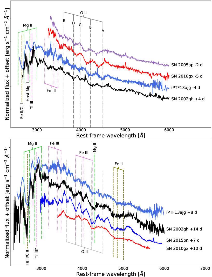
Figure 5: Comparison between the early phase spectra of SN 2002gh, SN 2005ap (Quimby et al., 2007), SN 2010gx (Pastorello et al., 2010), iPTF13ajg (Vreeswijk et al., 2014), and LSQ14bdq (Nicholl et al., 2015) (top panel), these SNe show the characteristic O ii spectral features in the 3500-5000 Å region. The vertical dot-dashed lines represent the effective wavelengths for the A, B, C, D, and E O ii spectral features identified by Quimby et al. (2018) at an expansion velocity of $10,000$ km s^-1. We identify and mark other ions with vertical lines such as the Ti iii $\lambda\,2984.747$ line identified by Mazzali et al. (2016), C ii, Mg ii, Fe ii and Fe iii lines at the same expansion velocity of $10,000$ km s^-1. We mark the host galaxy Mg ii $\lambda\lambda$ $2796,2803$ doublet absorption feature with a pink tick. On the bottom panel, we present the comparison between the post-maximum cooling phase spectra of SN 2002gh, SN 2010gx, iPTF13ajg, and SN 2015bn (Nicholl et al., 2016a). In addition to the correction by the host galaxy recession velocity, the spectrum of SN 2015bn has been shifted to the blue by 2500 km s^-1 to match the SN 2002gh spectrum at this phase. As in the top panel, the lines of several ions are marked and identified with vertical lines at an expansion velocity of 9500 km s^-1.

3.1.2 Cooling phase ($+4$ d $\textless t\lessapprox+15$ d)

The cooling begins at a few days after maximum and ends between 10 and 20 days past maximum. It is characterized by a decrease in the strength of the characteristic O ii lines, until they disappear at the end of this phase. This is a consequence of the decrease in the ionization state of the SN ejecta after maximum light. However, the SN ejecta remains hot enough for Fe iii features to take the place of O ii features, while the latter decrease their strength significantly. This evolution is reflected in: 1) O ii A and E features fade quicker than other O ii features after maximum, 2) the O ii C and D features, which are coincident with Fe iii lines, remain visible in the SN spectra for longer time than A and E features, and 3) in the meantime, the O ii B feature which is blended with Fe iii, Fe ii and Mg ii lines, increases its strength and quickly shifts to the red. At this phase, the O ii B feature exhibits a distinctive double absorption due to Fe iii in the blue and to Mg ii in the red. In the bottom panel of Fig. 5 we illustrate the Fe iii lines and the Mg ii $\lambda\,4446.31$ feature at an expansion velocity of $9500$ km s^-1 in the region previously dominated by O ii lines. These two minima can be clearly distinguished in SN 2015bn and SN 2010gx. Contemporary to this, Fe ii lines give shape to the broad spectral feature in the region between 4500-5250 Å (see bottom panel of Fig. 5).

As before, the Fe iii absorption features are tentatively distinguished in the spectra of iPTF13ajg and SN 2015bn in the region between $3100$ Å and $3500$. However, the identification of these features is less clear in SN 2002gh. We associate the feature at 3000 Å with Mg ii in SN 2002gh and in iPTF13ajg. The spectral feature at $2830$ Å is now shifted blueward in these SNe, in a better agreement with the Mg ii line rather than with the Ti iii line, suggesting a decrease in the contribution of the latter ion to this feature. We associate the strong 2670 Å feature with Fe ii and Mg ii lines, and note that the minimum of this feature is bluer in SN 2002gh. Possible explanations for this are; 1) a higher expansion velocity of the line producing this feature in SN 2002gh, 2) a contribution from an unidentified ion not present in the iPTF13ajg spectrum or 3) host galaxy absorption lines shifting the line to the blue as in the case of the Mg ii host galaxy absorption line that ‘shifts’ the 2830 Å feature to the blue. Several strong Fe ii lines on the blue side of this feature at the host galaxy rest-frame can be potentially identified, providing support to the latter possibility.

The spectra of SN 2002gh from +9 to +12 days are representative of the cooling phase. The average decrease of the SN 2002gh ejecta temperature is about 210 K per day, with an approximate ejecta temperature within the range of about $13,500$ to $11,000$ K in the course of this phase. We find that the spectra of SN 2002gh at this phase are similar to iPTF13ajg and SN 2015bn (after shifting the latter spectrum to the blue in Fig. 5 for a better comparison with the spectral features of SN 2002gh).

3.1.3 Post-maximum phase ($+15$ d $\lessapprox t\lessapprox+40$ d)

The beginning of the post-maximum phase can be defined as when high-ionization lines such as O ii and Fe iii lines vanish, and the dominant spectral features are produced by Fe ii, Mg ii and other IME’s. This happens at about 10 to 20 days after maximum. These changes make hydrogen-poor SLSNe exhibit spectral features similar to SNe Ic and Ic-BL at an early phase (Fig. 6), but the spectral features of SLSNe are shallower and have a bluer continuum.

In Fig. 6 we distinguish the 3800 Å feature produced by Mg ii and the H&K Ca ii lines, the 4315 Å feature produced by Mg ii and Fe ii lines and the broad feature between 4500-5250 Å produced mainly by Fe ii lines, but with contributions from other IME’s such as Mg ii. Notably, the 4315 Å feature has evolved from being produced by the O ii B feature, then produced by a combination of Fe iii, Fe ii and Mg ii with a distinctive double absorption feature such as in SN 2015bn and SN 2010gx, to a single absorption produced by Mg ii and Fe ii at this phase. Note that there is an Fe ii line close in wavelength to the Mg ii line in this feature, which we do not mark in Fig. 6 to avoid crowding. Additional Fe ii lines bluewards and redwards in wavelength also shape this feature.

At UV wavelengths, the spectral features at $2670$ Å and $2830$ Å remain, and Fe ii and Mg ii are the main suspects to explain these features. For first time the Ca ii features are detected, and they contribute to the spectral features at 3080 Å and 3800 Å blended with Mg ii lines (see Fig. 6). The spectra of SN 2002gh at +24 and +28 days are representative of this phase, where the ejecta expansion velocity is about $9000$ km s^-1 and $T_{\mathrm{bb}}\sim 10,500$ K.

3.1.4 Cool-photospheric phase ($t\textgreater+40$ d)

As the ejecta temperature decreases the resemblance of SLSNe to SNe Ic and Ic-BL becomes more evident, the pseudo-continuum becomes redder and the strengths of the lines increase, as can be seen in Fig. 6. When the ejecta temperature of SLSNe is about or below $10,000$ K the strength of the 4315 Å feature in SLSNe becomes similar to SNe Ic. This is the case of SN 2002gh from about +40 days, when the ejecta temperature is about $9500$ K and the ejecta expansion velocity is slightly below $9000$ km s^-1.

In Fig. 6, we notice that while the 4315 Å feature in SLSNe has reached a strength roughly similar as in the Ic SN 1994I, the spectral feature between 4500-5250 Å, although stronger than in previous phases, is shallower than in SNe Ic and Ic-BL. The UV emission has decreased due to the decline of the ejecta temperature and due to an increase of absorption from IME’s and Fe ii lines. The spectral features at $2670$ Å and $2830$ Å remain. The SLSN emission it is now slowly evolving towards the pseudo-nebular phase.

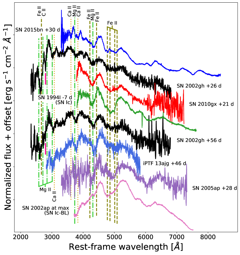
Figure 6: Post-maximum and cool-photospheric phase comparison. We mark and identify the lines of several ions with vertical lines at an expansion velocity of 9000 km s^-1. For comparison, we present the spectra of the Type Ic SN 1994I and the Type Ic-BL SN 2002ap (Modjaz et al., 2014), and the hydrogen-poor SLSN 2005ap, SN 2010gx, iPTF13agj, and SN 2015bn. As in Fig. 5, the spectrum of SN 2015bn has been shifted to the blue by 2500 km s^-1. As before, we highlight the Mg ii $\lambda\lambda$ $2796,2803$ doublet host galaxy absorption in SN 2002gh spectra with a pink tick.

3.2 Host galaxy characterization

The field of the SN explosion has been covered by several modern digital surveys over the past decades. With the aim of identifying and characterising the SN 2002gh host galaxy, we searched for host galaxy candidates close to the SN position in these deep surveys. The nearest astronomical source to the SN site detected by both SDSS and Pan-STARSS is galaxy G1 shown in Fig. 1, and already discussed in Section 2.

We queried the NOAO archive for DECam archival frames containing the SN region and after inspecting them, we noticed some faint emission close to the SN site on some of the individual DECam frames. However, the number of counts is too low to claim a detection on these individual frames. Therefore, to sum all possible photons, we stacked all $griz$ frames for each individual filter, and we also made a multi-band image stack with all the $griz$ frames using SWarp (Bertin et al., 2002). Figure 7 shows the result of the multi-band $griz$ image stack and a colour composite image made of the individual $g$, $r$, $z$ stacks.

On the multi-band image stack, we detected an extended object at $\sim 10\sigma$ flux level above the background with centroid equatorial coordinates of $\alpha=$03:05:29.47 $\delta=-$05:21:57.08 (J2000) located 0$\aas@@fstack{\prime\prime}$13 south-east from the SN location corresponding to a projected distance of 0.67 kpc, at the redshift of the SN. We did not detect this source in the $i$-band image stack. In the $g$-band deep stack, we detected this source at $\sim 9\sigma$ level. On the $r$-band deep stack we detected three faint sources within $\sim$ 1$\aas@@fstack{\prime\prime}$5 of the SN position. The first source is detected at $\sim 6\sigma$ and the peak of the emission is 1$\aas@@fstack{\prime\prime}$01 or at a projected distance of 5.14 kpc north-east from the galaxy centroid measured in the multi-band image stack. The central source is detected at $\sim 10\sigma$ level and is located 0$\aas@@fstack{\prime\prime}$08 or at a projected distance of 0.44 kpc to the north-west of the galaxy centroid, this is essentially coincident with the multi-band image centroid. Finally, the third source is detected at $\sim 8\sigma$ and the peak is 0$\aas@@fstack{\prime\prime}$96 or at a projected distance of 4.90 kpc to the south-west of the galaxy centroid. Although the latter source is not detected as a different source in the $g$-band, it is clear that there are two emission peaks in the $g$-band image stack, one coincident with the main central source and one coincident with the south-west source. The three sources detected in the $r$-band can be distinguished in the colour composite image on Fig. 7. In the $z$-band we detected a source at the $\sim 6\sigma$ level with the peak located 0$\aas@@fstack{\prime\prime}$36 or at a projected distance of 1.82 kpc to the north-east from the multi-band galaxy centroid. Again this is essentially coincident with the main multi-band image centroid. The $z$-band source is very weak and does not show evidence of structured emission. Although the small projected distance between the host galaxy candidate reported here and the SN is a strong reason to think that this is the SN host, further spectroscopic confirmation of the galaxy redshift is required for a solid association. The multi-peak morphology found in the SN 2002gh’s host candidate is common in hydrogen-poor SLSN host galaxies. Analysing Hubble Space Telescope images, Lunnan et al. (2015) found that roughly half of the hydrogen-poor SLSN host galaxies exhibit a morphology that is either asymmetric, off-centre or consisting of multiple peaks. Recently, Ørum et al. (2020) found that hydrogren-poor SLSN host galaxies are often part of interacting systems, with $\sim 50$% having at least one major companion within 5 kpc.

Assuming that the source detected is the SN host, we note that at this redshift the usual emission lines of SLSN-I host galaxies, such as [O ii] $\lambda\lambda$ $3726,3729$ doublet emission lines lie wthin the $g$ band, the H$\beta$ and the [O iii] $\lambda\lambda$ $4959,5007$ doublet emission lines lie within the $r$ band, and the H$\alpha$ and [S ii] $\lambda\lambda$ $6717,6731$ doublet emission lines lie within the $z$ band. These emission lines are strong in regions with recent or ongoing star-formation, in particular in Extreme Emission Line Galaxies (EELGs; e.g. Cardamone et al., 2009; Atek et al., 2011; Amorín et al., 2014, 2015), and therefore the peaks detected could be tracing regions of strong star-formation within the irregular host or could simply mean that these are different dwarf galaxies in the merging process. Leloudas et al. (2015) showed that hydrogen-poor SLSNe hosts are found in environments where the gas is strongly ionized, more than in stripped CCSN hosts, and have stronger [O iii] $\lambda 5007$ emission lines compared to the hosts of other transients types, but comparable to EELGs.

We performed aperture photometry using SExtractor (Bertin & Arnouts, 1996), and we calibrated against $griz$ magnitudes of stars C2, C3, C4, C6 and C7 in Fig. 1 from SDSS. We summarize the host galaxy photometry in Table 4.

Table 4: DECam $griz$ photometry for the SN 2002gh host galaxy.

Filter	mag	Abs. mag
$g$	$24.3$($0.2$)	$-17.3$
$r$	$23.5$($0.1$)	$-18.2$
$i$	>$24.1$	>$-17.5$
$z$	$23.3$($0.3$)	$-18.3$

• Numbers in parentheses correspond to 1 $\sigma$ statistical uncertainties.

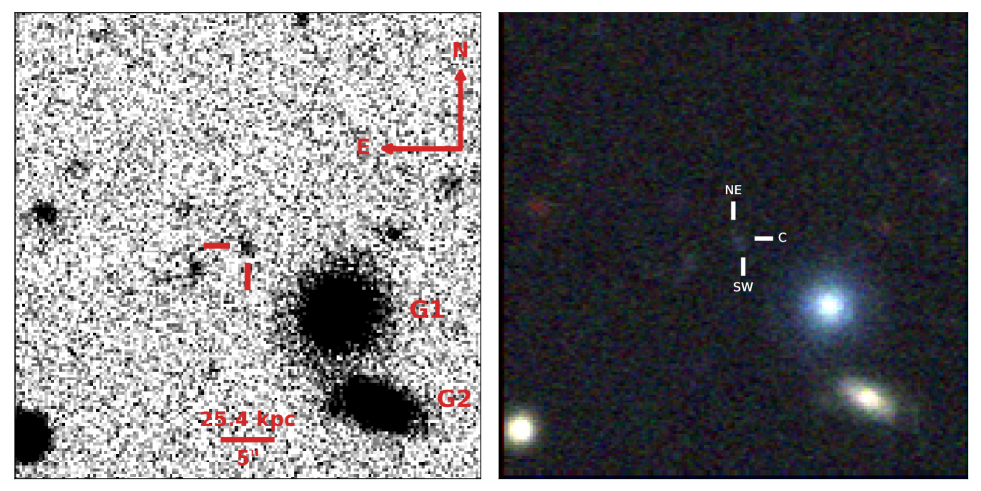
Figure 7: In the left panel, we present a greyscale image centred on the position of SN 2002gh, resulting from stacking all the $griz$ DECam frames available. We indicate the host galaxy position with red tick marks, and we label the foreground galaxies G1 and G2. In the right panel, we present a $grz$ colour image composite made of deep image stacks in these filters. In the colour image, the position of the north-east, central and south-west faint distinct components detected in the $r$ band associated to potential host galaxy of SN 2002gh, are indicated with a white tick marks. The field-of-view of both images is 0$\aas@@fstack{\prime}$72 $\times$ 0$\aas@@fstack{\prime}$72, and at the bottom of the left panel we give as reference the projected physical distance of 5$\aas@@fstack{\prime\prime}$0 at the SN redshift.

3.3 Light curve characterization

SN 2002gh was discovered a few weeks before the epoch of maximum bolometric luminosity (see Section 3.4), and our observations begin six days before bolometric maximum in the rest-frame. We distinguish four phases in the light curve evolution of SN 2002gh in Fig. 3. The first phase corresponds to the light curve evolution close to maximum light, a second phase of decline post-maximum until 70 days after maximum, a third phase of faster decline between days 69-105 days, and a fourth phase between 100-205 days, for which we only have observations in the $V$-band.

The optical observations presented here begin shortly before maximum brightness in the $VRI$ bands, and after $B$-band maximum. The $I$-band observations show a bumpy structure close to peak, which is caused by a lower signal-to-noise photometry in this band. To estimate the epoch and the brightness at maximum light in $VRI$ bands, we used the Gaussian process interpolation. An upper limit on the MJD of the $B$-band maximum and the in the magnitude at this epoch was placed. The uncertainty in the time of maximum light corresponds to the time difference between the epoch of the maximum from the Gaussian process interpolation, and the epoch of the brightest photometric observation (synthetic photometry for the $R$ band). The uncertainty in the maximum brightness is the difference between the brightest value in the Gaussian process interpolation and the brightest photometric observation in the corresponding band. These values are summarized in Table 5.

A first order polynomial was fitted to the post-peak photometric observations in the $BVI$ filters and to the $R-$band sythetic photometry. The goodness-of-fit of these linear models was estimated by computing $\chi^{2}_{\nu}$ and the root mean squared (rms) of the fit. Inspecting the fit residuals, we find that a first order polynomial is a suitable model over these limited ranges of time. The values for the decline rates, $\chi^{2}_{\nu}$, and the rms are summarized in Table 6.

During this second phase, spanning from after peak brightness ($t\textgreater 15$ days) to 70 days after bolometric maximum, the SN luminosity declined more rapidly in the bluer bands with decline rates of 1.82, 1.31, 0.98 and 0.79 mags/100 days in $B$, $V$, $R$, $I$, respectively. In particular, we notice that the $B$-band declined two times faster than the $I$-band, at the 4 $\sigma$ level, pointing to a rapid decrease of the UV emission after maximum due to a decrease of the ejecta temperature, as a consequence of which there is an increase in the strength of the absorption lines mainly due to Fe ii and intermediate-mass elements (IME’s), as we discussed above (see Section 3.1).

In the third phase, from 69 to 105 days after maximum brightness, we found that the decline rates increase to 4.24, 2.95 and 3.32 mags/100 days in $B$, $V$, $I$ bands, respectively. This is an increase by a factor of 2.3, 2.2 and 4.2, respectively, compared to the decline rates in previous phase in the same bands. Note the rapid decline in the $B$ band which is larger by $1.3\pm 0.3$ mag/100 days (4 $\sigma$) compared to the $V$-band decline rate. This implies a rapid fading of the near-UV emission. The $V$ and $I$ decline rates are similar at this phase within 1 $\sigma$. We notice that all the decline rates are faster than the expected decline of $\sim 1$ mag/100 days for a SN powered by the radioactive decay of ⁵⁶Co, the daughter product of ⁵⁶Ni. The decline rate in the $V$ band in the fourth phase was measured by fitting a linear model to the last three photometric observations in this band, finding a value of $1.33\pm 0.17$ mags/100 days. Although there is a gap of nearly 100 days between the first point and the last two points, the $V$ band slowed its decline rate to less than half of its previous phase value, at the 7.5 $\sigma$ level. This provides evidence of a flattening in the light curve at this late phase.

Table 5: Peak magnitude information for SN 2002gh.

Filter	MJD peak	Peak	Peak abs.
	(days)	magnitude	magnitude
$B$	$\leq 52576.8$	$\leq 19.48$	$\leq-22.22$
$V$	$52568.8$($3.4$)	$19.24$($0.04$)	$-22.40$
$R$	$52574.8$($2.2$)	$19.11$($0.05$)	$-22.49$
$I$	$52569$($26$)	$19.04$($0.09$)	$-22.51$

• Numbers in parentheses correspond to 1 $\sigma$ statistical uncertainties.

Table 6: Decline rates in the optical bands for SN 2002gh.

Filter	Dec. rate phase 1	$\chi^{2}_{\nu}$	$\mathrm{\it rms}$	$n_{\mathrm{obs}}$	Dec. rate phase 2	$\chi^{2}_{\nu}$	$\mathrm{\it rms}$	$n_{\mathrm{obs}}$	Dec. rate phase 3	$\chi^{2}_{\nu}$	$\mathrm{\it rms}$	$n_{\mathrm{obs}}$
	(mag/100 days)		(mag)		(mag/100 days)		(mag)		(mag/100 days)		(mag)
$B$	$1.82$($0.09$)	$0.71$	$0.030$	$5$	$4.24$($0.29$)	–	–	$2$	–	–	–	–
$V$	$1.31$($0.06$)	$0.04$	$0.006$	$5$	$2.95$($0.17$)	$0.13$	$0.013$	$5$	$1.33$($0.17$)	$0.38$	$0.064$	$3$
$R$	$0.98$($0.98$)	$0.03$	$0.006$	$3$	–	–	–	–	–	–	–	–
$I$	$0.79$($0.10$)	$1.99$	$0.056$	$5$	$3.32$($0.29$)	$1.22$	$0.045$	$4$	–	–	–	–

• Numbers in parentheses correspond to 1 $\sigma$ statistical uncertainties.

3.4 Blackbody fits, bolometric and pseudo-bolometric light curves

The spectral energy distribution (SED) of hydrogen-poor SLSNe can be well described by a blackbody model from the time of explosion to a few days or weeks after maximum light (e.g., Nicholl et al., 2017). After maximum light, the SLSN emission becomes progressively dominated by broad features similar to broad-line SNe Ic (Liu et al., 2017), and then enter progressively in the nebular phase (Jerkstrand et al., 2017; Nicholl et al., 2016b; Nicholl et al., 2019).

To estimate the radius and the temperature of the SN ejecta we fitted a modified blackbody model to the interpolated $VRI$ photometry of SN 2002gh corrected by Galactic extinction. The conversion from magnitudes in the Vega photometric system to monochromatic fluxes was done using the zero points listed in the Table A2 of Bessell et al. (1998). The modified blackbody function employed to compute the SN bolometric luminosity, corresponds to a Planck function with a linear flux suppression below the “cutoff” wavelength at 3000 Å as shown in Fig. 4 and is described in the Appendix. To complement $V$ and $I$ bands in the blackbody fits, we used $R-$band synthetic photometry and extrapolated this band by about 50 days using the Gaussian process model shown in Fig. 3. We compared fits obtained from $VRI$ and $VI$ photometry, and found that both methods yield similar results. We noticed that the addition of $R-$band synthetic photometry brings the blackbody parameters closer to the values estimated from fitting a blackbody to the SN spectra (see Figs. 4 and 8).

We did not include $B$-band photometry in our blackbody fits as this band is affected by strong absorptions from about +14 days after maximum, as can be seen in Fig. 4 and discussed in Sections 3.3 and 3.1. To study this effect, we compared the blackbody parameters obtained by fitting a blackbody model to the $BVRI$ and to the $VRI$ photometry. At early times (<+14  days) the $B-$band emission is not significantly affected by strong spectral features and the derived blackbody parameters obtained including $B$-band photometry yield an excellent match with the blackbody computed using $VRI$ photometry and with the SN spectra. After this, the $B$ band becomes progressively affected by the decrease in the ejecta temperature (Section 3.1), showing clear differences between the blackbody temperature and radius computed with and without including the $B$-band. However, in all cases we find a good agreement in the bolometric luminosity. We decided to use $VRI$ to perfom the blackbody fits because it yields the most reliable and consistent blackbody parameters at all epochs.

The blackbody fits were performed by $\chi$-square minimization and assuming a luminosity distance of $1,951.7$ Mpc, which yielded three physical parameters for each epoch: the blackbody temperature ($T_{\mathrm{bb}}$), radius ($R_{bb}$) and the bolometric luminosity. To estimate the uncertainty in these parameters a Monte Carlo simulation was performed, where we simulate $15,000$ times a new set of photometric points assuming a Gaussian distribution with the standard deviation equal to the photometric uncertainty, and the blackbody parameters were re-computed obtaining a distribution for each of them. From the distribution obtained for $T_{bb}$ and $R_{bb}$, lower and upper $1\sigma$ limits were computed (Fig. 8). Using the blackbody parameters and their uncertanties, we then computed the bolometric luminosity ($L_{\mathrm{bol}}$) and its uncertainty. The observed optical luminosity ($L_{BVRI}$) was estimated summing the emission in the $BVRI$ bands (see Fig. 8).

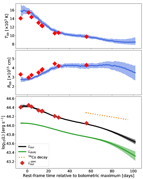
Figure 8: Blackbody parameters, bolometric and observed optical luminosity light curves for SN 2002gh. In the top and middle panel we present the blackbody temperature $T_{\mathrm{bb}}$ and radius $R_{\mathrm{bb}}$ obtained from the blackbody fits to the $VRI$ interpolated photometry of SN 2002gh (blue line) and to the spectra (red diamonds; see Fig 4). In the bottom panel, we present the $L_{\mathrm{bol}}$ (black) and $L_{BVRI}$ (green) light curves and compare them with the decline rate of ⁵⁶Co. We also present the individual points computed from the blackdody fits to the spectra for $L_{\mathrm{bol}}$ (red diamonds).

The peak of the bolometric emission was on $\mathrm{MJD}=52570.8\pm 2.4$ days with a luminosity of $2.6\pm 0.1\times 10^{44}$ erg s^-1 ($log_{10}(L^{\mathrm{peak}}_{\mathrm{bol}})\simeq 44.4$). This value places SN 2002gh among the brightest of SLSNe, with only a handful of objects reaching brighter peak bolometric luminosities as we discuss below. The peak of the observed luminosity was on $\mathrm{MJD}=52564.3\pm 1.5$ days, reaching a luminosity of $1.13\pm 0.03\times 10^{44}$ erg s^-1 ($log_{10}(L^{\mathrm{peak}}_{\mathrm{BVRI}})\simeq 44.0$). The ratio between the bolometric luminosity and the luminosity observed in the optical bands is $L^{\mathrm{peak}}_{\mathrm{bol}}/L^{\mathrm{peak}}_{\mathrm{BVRI}}=2.3\pm 0.1$.

We estimate that the total radiated energy from $-6$ to $+102$ days is $1.2\times 10^{51}$ erg, and a total radiated energy observable in the optical bands of $6.1\times 10^{50}$ erg, over the same period of time. These values represent a lower limit to the energy emitted by the SN.

The decline rates of the bolometric and pseudo-bolometric light curves over the phase from 15 to 70 days and from 70 days to the end of the light curves ($\simeq 100$ days) were measured. These ranges are equivalent to the second and third phases analysed in the previous section, however, here we use interpolated light curve values while in Section 3.3 we used individual photometric observations. These luminosity decline rates in magnitudes declined over 100 days are summarized in Table 7. Note that the decline rate during the first phase (15 to 70 days) is more rapid than the decline rate expected for a light curve powered by the ⁵⁶Co $\rightarrow$ ⁵⁶Fe decay, but it could be still consistent with the ⁵⁶Co decay. However, the decline rate measured for the second phase ($t$ >+70 days) is 2.4 times faster than the expected decline rate for a ⁵⁶Co powered light curve. This suggests that the decay of ⁵⁶Ni is not the main power source of SN 2002gh. This will be dicussed in detail in Section 3.5.2 below.

While the $L_{\mathrm{bol}}$ computation assumes a blackbody SED, which does not hold at all epochs, particularly at late phases, $L_{\mathrm{bol}}$ and $L_{BVRI}$ decline rates are in very good agreement, specially at $t$ >+70 days. We also note that over similar phases the $L_{\mathrm{bol}}$ decline rates are similar to the $V$-band decline rates presented in Table 6.

Table 7: Luminosity decline rates of SN 2002gh.

Light curve	Dec. rate at +15 d <ph <+70 d	Dec. rate at ph >+70 d
	(mag/100 days)	(mag/100 days)
$L_{\mathrm{bol}}$	$1.49$($0.02$)	$2.38$($0.11$)
$L_{BVRI}$	$1.44$($0.02$)	$2.38$($0.22$)

• Numbers in parentheses correspond to 1 $\sigma$ statistical uncertainties.

3.4.1 Luminosity comparison

It has been shown that SN 2002gh is a bright SN belonging to the SLSN class. However, at this point it is unclear how bright the event is relative to other SLSNe. In this section, the bolometric light curve of SN 2002gh is compared with a large sample of SLSNe, placing this object in the context of the SLSN population as a whole. To this end, a set of bolometric light curves are computed, using photometry from spectrocopically confirmed hydrogen-poor SLSNe from Pan-STARRS1 (PS1; Lunnan et al., 2018) and the Dark Energy Survey (DES; Angus et al., 2019). The large PTF SLSN sample (De Cia et al., 2018) is not included in this analysis as their multi-band photometry is not uniform accross their entire sample, thus making it difficult to construct a homogeneus set of bolometric light curves. Well observed objects from the literature are not included in our sample of bolometric light curves either, as individual objects suffer from biases that can be difficult to account for. Note that the PS1 and DES SLSN samples suffer from spectroscopic selection biases, inherent to any spectroscopic sample, which are dicussed by Lunnan et al. (2018) and Angus et al. (2019), respectively. Nevertheless, these two SLSN samples represent a well characterized data set, with well defined photometric systems, providing a uniform and deep multi-band photometry ($griz$), thus perfect for contructing bolometric light curves. The redshift ranges are $0.3\lesssim z\lesssim 1.6$ for the PS1 sample and $0.2\lesssim z\lesssim 2.0$ for the DES sample.

The rest-frame optical and NIR is the spectral region of choice for fitting a blackbody SED to SLSNe. For this reason we restrict ourselfs to construct bolometric light curves for objects at $z\lesssim 1.2$. This choice is justified in the Appendix.

In the left-panel of Fig. 9, the bolometric light curves of 28 SLSNe-I, 11 from PS1 and 17 from DES, are presented and compared with the bolometric light curve of SN 2002gh. As can be observed SN 2002gh reaches one the largest maximum luminosities of this sample, with only two SNe from PS1 reaching similar values. Note that PS1 SLSNe are concentrated in the bright region of the distribution compared with DES objects, having a maximum bolometric luminosity range of $log_{\mathrm{10}}(L_{\mathrm{bol}})=43.5-44.4$. The DES SLSNe span a wider luminosity range with $log_{\mathrm{10}}(L_{\mathrm{bol}})=43.25-44.3$. This is likely explained in part by the fact that the DES survey limiting magnitude, in terms of photometry and spectroscopy, reaches nearly 1 mag fainter than the PS1 survey. As can be noticed in the figure there is a large diversity in the shape of the light curves, with some objects having early bumps and others showing bumps after maximum light. We also find a large diversity in the rise times with objects having rise times of about 30 days and others showing broader light curves, with PS1-14bj being an extreme object with a rise time of more than 100 days. No apparent relation between the peak luminosity and the light curve shape is found.

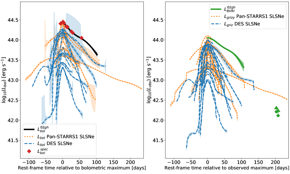
Figure 9: Bolometric and observed luminosity light curve comparison between SN 2002gh and the spectroscopically confirmed SLSNe from Pan-STARRS1 (Lunnan et al., 2018) and DES (Angus et al., 2019). In the left panel, we present the bolometric light curves and in the right panel we present the emitted luminosity detected in the optical bands. In the Appendix we describe our methodology to compute bolometric and observed luminosity light curves in detail.

In the right-panel of Fig. 9 the luminosity light curves for PS1 and DES SLSNe constructed by adding the emission detected in the optical bands are presented. Here the sample is not restricted to objects with $z\lesssim 1.2$, thus all PS1 and DES objects are included. SN 2002gh is again among the brightest SLSNe, only PS1-13or ($z=1.53$) reaches a brighter maximum luminosity. Here again PS1 SLSNe are concentrated in a brighter region compared with DES objects, which are distributed over a wider luminosity range.

In Fig. 10 the maximum bolometric luminosity distribution is presented for spectroscopically confirmed hydrogen-poor SLSNe from PS1 and DES. This distribution includes all possible PS1 and DES objects, 37 SLSNe in total. For objects at $z\textgreater 1.2$, we estimate the maximum bolometric luminosity using the heuristic $L_{\mathrm{bol}}/L_{\mathrm{obs}}$ scaling relation described in the Apendix. Only PS1-10awh ($z=0.909$), PS1-11bam ($z=1.565$), PS1-13or ($z=1.53$), and DES15E2mlf ($z=1.861$) have a similar or brighter maximum luminosity than SN 2002gh. This figure confirms that SN 2002gh lies at the extreme of the distribution, only comparable to the most luminous objects in a sample of 37 SLSNe, which includes the most distant and luminous objects detected to date.

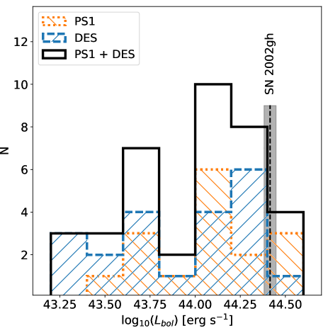
Figure 10: Observed maximum bolometric luminosity distribution for spectroscopically confirmed SLSNe from Pan-STARRS1 (Lunnan et al., 2018) and DES (Angus et al., 2019). This distribution includes peak bolometric luminosity for objects at $z\textgreater 1.2$, which are estimated using a heuristic method described in the Appendix. We mark with a black dashed line the maximum bolometric luminosity of SN 2002gh, confirming that it is among the most luminous SNe ever observed.

3.5 Power source

In this Section the magnetar model together with radioactive decay of ⁵⁶Ni are explored as possible sources to power the extreme luminosity of SN 2002gh. We also discuss potential signatures of interaction between the SN ejecta and the CSM.

3.5.1 Magnetar model

The power injection from the spin down of a newborn magnetar is a theoretical model able to explain the extreme luminosities of hydrogen-poor SLSNe. Under the assumption that SN 2002gh is powered by the spin down of a magnetar, here we use the magnetar model implemented by Nicholl et al. (2017) to fit the photometry of SN 2002gh using two methodologies: 1) the Modular Open Source Fitter for Transients (MOSFiT; Guillochon et al., 2018) that uses the SN photometry as input, and 2) our python implementation of the model to fit the bolometric light curve directly.

Here we briefly summarize the main analytic expresions of the magnetar model of Nicholl et al. (2017). We refer the reader to this article and the references therein for a detailed description of the model. The magnetar energy input ($F_{\mathrm{mag}}$) is:

$$F_{\mathrm{mag}}(t)=\frac{E_{\mathrm{mag}}}{t_{\mathrm{mag}}}\frac{1}{(1+t/t_{\mathrm{mag}})^{2}},$$ (1)

where the magnetar rotational energy ($E_{\mathrm{mag}}$) is

$$E_{\mathrm{mag}}=2.6\times 10^{52}\left(\frac{M_{\mathrm{NS}}}{1.4~{}M_{\sun}}\right)^{3/2}\left(\frac{P_{\mathrm{spin}}}{1~{}\mathrm{ms}}\right)^{-2}\mathrm{erg,}$$ (2)

the magnetar spin down timescale ($t_{\mathrm{mag}}$) is given by

$$t_{\mathrm{mag}}=1.3\times 10^{5}\left(\frac{M_{\mathrm{NS}}}{1.4~{}M_{\sun}}\right)^{3/2}\left(\frac{P_{\mathrm{spin}}}{1~{}\mathrm{ms}}\right)^{2}\left(\frac{B}{10^{14}~{}\mathrm{G}}\right)^{-2}\mathrm{s.}$$ (3)

In these expressions $M_{\mathrm{NS}}$, $P_{\mathrm{spin}}$, and $B$ correspond to the mass, spin period, and magnetic field of the neutron star, respectively.

The output SN luminosity ($L_{\mathrm{SN}}$) is calculated using the traditional analytic solution of Arnett (1982), where in this case the SN energy source is $F_{\mathrm{mag}}(t)$ and the analytic expression takes the following form:

$$L_{\mathrm{SN}}(t)=e^{-(t/t_{\mathrm{diff}})^{2}}(1-e^{-At^{-2}})\int\limits_{0}^{t}2~{}F_{\mathrm{mag}}(t^{\prime})\frac{t^{\prime}}{t_{\mathrm{diff}}}e^{(t^{\prime}/t_{\mathrm{diff}})^{2}}\frac{dt^{\prime}}{t_{\mathrm{diff}}},$$ (4)

where the diffusion timescale is given by

$$t_{\mathrm{diff}}=\left(\frac{2\kappa M_{\mathrm{ej}}}{\beta cv_{\mathrm{ej}}}\right)^{1/2},$$ (5)

and includes a leakage parameter (Wang et al., 2015; Nicholl et al., 2017), not included in the original Arnett (1982) analytic expression, of the form:

$$A=\frac{3\kappa_{\gamma}M_{\mathrm{ej}}}{4\pi v^{2}_{\mathrm{ej}}}.$$ (6)

In these expressions the parameter $\beta$ has the typical value of 13.7 (Arnett, 1982; Inserra et al., 2013), $c$ is the speed of light, $M_{\mathrm{ej}}$ is the ejecta mass, $v_{\mathrm{ej}}$ is the characteristic ejecta velocity, $\kappa$ is the optical opacity, and $\kappa_{\gamma}$ is the opacity to high-energy photons. The leakage term, $(1-e^{-At^{-2}})$, controls the fraction of high-energy photons thermalized by the SN ejecta (Wang et al., 2015; Nicholl et al., 2017). A large value of $\kappa_{\gamma}$ implies a significant thermalization of the magnetar input energy at all times, while a small $\kappa_{\gamma}$ value implies that a large fraction of the magnetar energy escapes in the form of high energy radiation at late times (Wang et al., 2015; Vurm & Metzger, 2021), when the ejecta density drops.

In Fig. 11 we present the MOSFiT magnetar model fit result for SN 2002gh, where we fixed $z=0.365$ and the Galactic reddening to $E(B-V)=0.0593$ mag in the fit. We do not allow MOSFiT to fit for host galaxy extinction or the gas column density parameters. Note that this fit describes reasonably well the light curve evolution, including the late $V$-band photometry, with the most significant discrepancies in the $B$ and $I$ bands. We used additional information obtained from the analysis of SN 2002gh spectra presented in Section 3.1 to set restrictions on $v_{\mathrm{ej}}$. In Section 3.1, we measured an ejecta expansion velocity between $9000$ and $11,000$ km s^-1 over a rest-frame time of more that 60 days. Over this time interval we probed several layers of the SN ejecta, quantifying changes in the ejecta temperature and velocity. Therefore, it is expected that our estimate for the SN expansion velocity should be representative of the ejecta velocity. For this reason, a Gaussian prior on $v_{\mathrm{ej}}$ is employed, having a mean velocity of $10,000$ km s^-1 and a standard deviation of $1000$ km s^-1. Additionally, the following restriction $7,000\textless v_{ej}\textless 16,000$ km s^-1 was imposed. Without these restrictions a value of $v_{ej}\simeq 5800$ km s^-1 would be obtained. This $v_{\mathrm{ej}}$ value represents 60% of the expansion velocity estimated from the minima of the spectral features in Section 3.1. The best MOSFiT values the for SN 2002gh are summarized in Table 8. We highlight the large ejecta mass of $M_{ej}\simeq 25\,M_{\sun}$ obtained by MOSFiT, and note that similar $M_{\mathrm{ej}}$ values are obtained regardless of the restrictions on $v_{\mathrm{ej}}$.

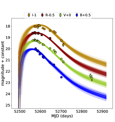
Figure 11: Magnetar model fit to SN 2002gh photometry using the Nicholl et al. (2017) implementation in MOSFiT (Guillochon et al., 2018).

Fig. 12 shows the analytic luminosity for the magnetar model using the MOSFiT parameters obtained for SN 2002gh, and compared with the bolometric light curve computed for SN 2002gh in the previous Section. There is an overall agreement between the two, but with the MOSFiT analytic light curve shifted by 0.10 to 0.15 dex to fainter luminosities than our estimated bolometric light curve. This shift is the result of differences in the methodologies employed to fit the modified blackbody model to the photometry and in the fitting procedure of the magnetar model itself. MOSFiT uses a Markov chain Monte Carlo (MCMC) fitter, to fit simultaneously for all the parameters in their model, including the photospheric velocity ($v_{\mathrm{phot}}$) and the final plateau temperature ($T_{f}$) which determine the blackbody temperature and radius evolution. In our case the evolution of the temperature and radius are not parameterized but fitted at each epoch independently. Another difference is the inclusion of the $B$ band photometry in the fit, which in our case does not yield significant differences in the bolometric emission, but which under a different fitting methodology and a different implementation of the modified blackbody emission may be a source of systematic discrepancies. Additionally, the MOSFiT light curve fit includes the late time $V-$band photometry at $200$ days, while the bolometric light curve ends at about $100$ days after the bolometric maximum. The two methodologies use a slighly different version of the Galactic reddening law to account for the Galactic extiction, which may introduce a small but systematic difference in the same direction observed. The MOSFiT analytic luminosity light curve peaks at about five days before the estimated epoch of the bolometric maximum, having a bolometric maximum luminosity of $1.5\times 10^{44}$ erg s^-1 ($log_{\mathrm{10}}(L_{\mathrm{bol}})=44.17$). This value represents 57.7% of the maximum luminosity estimated for SN 2002gh. Despite the constraints imposed on $v_{\mathrm{ej}}$, MOSFiT still tends to converge to a low ejecta velocity.

Motivated by these small but apparent discrepancies, we decided to explore a wide parameter space and fit directly the bolometric light curve of SN 2002gh using consistently the Nicholl et al. (2017) magnetar model implementation. To simplify the model and to reduce the number of parameters to fit, we decided to fix the velocity to $v_{\mathrm{ej}}=10,000$ km s^-1, and the neutron star mass to $M_{\mathrm{NS}}=1.7$ $M_{\sun}$ for a direct comparison with the MOSFiT fit. We also discuss the case of $M_{\mathrm{NS}}=1.4$ $M_{\sun}$ below. These values represent reasonable simplifiying assumptions. Our strategy consists in assessing a wide range of parameters that reasonably reproduce the bolometric light curve of SN 2002gh. To this we used a grid over a large range in $M_{\mathrm{ej}}$, $B$, $P_{\mathrm{spin}}$, and $\kappa$ and performed a least-squares minimization for $t_{\mathrm{exp}}$, and $\kappa_{\gamma}$ parameters to fit the bolometric light curve of SN 2002gh. The ranges explored for $M_{\mathrm{ej}}$, $B$, and $P_{\mathrm{spin}}$ are $0.63\leq M_{\mathrm{ej}}\textless 50.0~{}M_{\sun}$ with a logarithmic step of $log_{\mathrm{10}}(\Delta M_{ej})=0.1$, $0.1\leq B\textless 12.5\times 10^{14}~{}\mathrm{G}$ with a logarithmic step of $log_{\mathrm{10}}(\Delta B)=0.1$, $0.60\leq P_{\mathrm{spin}}\textless 7.25~{}\mathrm{ms}$ with a linear step of $\Delta P_{\mathrm{spin}}=0.20$ ms, and $0.1\leq\kappa\leq 0.2$ cm² gr^-1 with a linear step of $\Delta\kappa=0.025$ cm² gr^-1 respectively. Our motivation here is to explore the magnetar parameter space and find the sets of values able to reproduce the bolometric light curve of SN 2002gh, not only the set that yields the best fit.

The $\chi^{2}_{\nu}$ computed for each set of parameters was used to find good fits satisfying the energy balance requirement, that is $E_{K}\textless E_{\mathrm{mag}}-E_{\mathrm{rad}}+E_{\nu}$ (see Nicholl et al., 2017). Where $E_{K}$ ($=\frac{1}{2}M_{\mathrm{ej}}v^{2}_{\mathrm{ej}}$) is the kinetic energy of the SN ejecta, $E_{\mathrm{mag}}$ is the magnetar rotational energy, $E_{\mathrm{rad}}$ is the energy radiated and $E_{\nu}\approx 10^{51}$ erg is the canonical energy of a core-collapse explosion. Then, we selected the fits satisfying the energy balance and that also have $\chi^{2}_{\nu}\textless 20$. This $\chi^{2}_{\nu}$ value was selected after visual inspection of the fits, providing a good threshold for reasonable fits.

Our exploration found two clearly distinct groups in the parameter space clustered around lower $\chi^{2}_{\nu}$ values, that reproduce the bolometric light curve of SN 2002gh. These two groups can be mainly distinguished by their ejecta mass and the need of a leakage parameter. The best magnetar parameters for these solutions are summarized in Table 8. We found that the best fits correspond to an ejecta mass in the range of 0.6 to 3.2 $M_{\sun}$, $\kappa_{\gamma}$ between 0.16 and 0.53 cm² gr^-1, $\kappa$ between 0.1 and 0.2 cm² gr^-1, $P_{\mathrm{spin}}$ in the range 2.8-3.4 ms, and $B=0.50\times 10^{14}$ G. These fits have a $\chi^{2}_{\nu}$ between 2.02 and 2.18, and $\kappa$ varies proportional to $\kappa_{\gamma}$ and inversely proportional to the ejecta mass. The best fit is presented in the middle-panel of Fig. 12. The maximum luminosity of this model is $2.8\times 10^{44}$ erg s^-1, consistent with our estimate, the rise time to maximum luminosity is 24.9 days, this corresponds to about 10 days before the estimated epoch of maximum bolometric luminosity in the rest-frame. Starting at about 100 days after the explosion, we see that a noticeable fraction of the magnetar input energy leaks from the ejecta without being thermalized. This epoch corresponds to $60-70$ days after our estimated epoch of bolometric maximum (MJD=52570.8), and corresponds to the phase of rapid decline of the bolometric light curve.

The second set of solutions corresponds to a local minima and is characterized by a huge ejecta mass between about 30 and 40 $M_{\sun}$, having $\kappa_{\gamma}\textgreater 1.0$ cm² gr^-1. This set of solutions has problems to reproduce the maximum of the bolometric light curve as is also the case of the MOSFiT fit (see Fig. 12), having as a consequence larger $\chi^{2}_{\nu}$ values. Note that the huge ejecta mass together with $\kappa_{\gamma}\textgreater 0.1$ cm² gr^-1, implies that the energy leakage is negligible and these solutions are equivalent to the case of no leakage. In these fits, the spin period is between 0.6 and 1.0 ms, the magnetic field is between 1.6 and 2.0$\times 10^{14}$ G, $\kappa$ is between 0.175 and 0.2 cm² gr^-1, and the best solutions for this case have $\chi^{2}_{\nu}\simeq 10$. The rise time from the SN explosion to maximum luminosity is about 40 days, which corresponds to about six days before the estimated epoch of the bolometric maximum. This model has a maximum luminosity of about $2.0\times 10^{44}$ erg s^-1. The parameters for this case are in good agreement with the MOSFiT values, within the uncertainties (see Table 8). The agreement can be considered even better if the systematic differences between the two methodologies employed are considered. Hence, we consider the MOSFiT solution equivalent to our best bolometric fit without leakage.

The mass function of neutron stars show evidence of a bimodal distribution, with a low-mass component centred at $1.4M_{\sun}$, and a high-mass component centred at $1.8M_{\sun}$ (Antoniadis et al., 2016). To investigate the effect of the neutron star mass in our results we fitted the bolometric light curve of SN 2002gh fixing $M_{\mathrm{NS}}=1.4M_{\sun}$. We found that both solutions remain in this case, and as in the case of $M_{\mathrm{NS}}=1.8M_{\sun}$ the second solution is found when $\kappa$ is between 0.175 and 0.2 cm² gr^-1. In Table 8 we summarize the parameters for the best fits in each case. The values change slightly compared with the $M_{\mathrm{NS}}=1.7M_{\sun}$ case, but are still consistent with the previous results.

Table 8: Parameters of the magnetar model fits of SN 2002gh.

Magnetar parameters	$M_{\mathrm{ej}}$	$v_{\mathrm{ej}}$	$P_{\mathrm{spin}}$	$B$	$\kappa$	$\kappa_{\gamma}$	$M_{\mathrm{NS}}$	$\chi^{2}_{\nu}$
	($M_{\sun}$)	($\times 10^{3}$ km s-1)	(m s)	($\times 10^{14}$ G)	(cm2 gr-1)	(cm2 gr-1)	($M_{\sun}$)
MOSFiT	$25.1^{+5.1}_{-3.7}$	$7.8^{+0.6}_{-0.6}$	$1.2^{+0.2}_{-0.2}$	$1.9^{+3.8}_{-1.1}$	$0.17^{+0.02}_{-0.03}$	$6.0^{+125.8}_{-5.7}$	$1.7^{+0.2}_{-0.3}$	–
Bolometric fit no leakage	$31.6$	$10.0^{\dagger}$	$1.0$	$1.6$	$0.200$	$\infty$	$1.7^{\dagger}$	10.1
	$31.6$	$10.0^{\dagger}$	$0.6$	$1.2$	$0.200$	$\infty$	$1.4^{\dagger}$	10.9
Bolometric fit with leakage	$2.0$	$10.0^{\dagger}$	$3.2$	$0.5$	$0.100$	$0.22$	$1.7^{\dagger}$	2.0
	$1.0$	$10.0^{\dagger}$	$3.0$	$0.4$	$0.100$	$0.38$	$1.4^{\dagger}$	1.6

• ^†Fixed values.

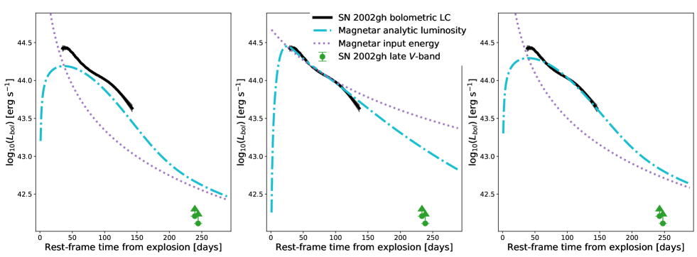
Figure 12: Left panel: comparison between the MOSFiT analytic bolometric light curve (cyan dash-dotted line) and the observed bolometric light curve of SN 2002gh (black continuous). Note that MOSFiT fits the magnetar model to the photometry directly, and not to the observed bolometric light curve of SN 2002gh shown in this panel. In all the panels, the purple dotted line represents the magnetar input energy to the SN ejecta, and the green circles are the late time $V$-band photometry of SN 2002gh which provide a lower limit for the SN bolometric luminosity at this phase. Middle panel: best magnetar fit to the bolometric light curve of SN 2002gh using our grid exploration method and including leakage. Right panel: best magnetar fit to the bolometric light curve of SN 2002gh without energy leakage.

3.5.2 Radioactive decay of ⁵⁶Ni

Here we explore the radioactive decay of ⁵⁶Ni as the possible power source for the light curve of SN 2002gh. The input energy from the ⁵⁶Ni radioactive decay (see Nadyozhin, 1994) is:

$$F_{\mathrm{Ni}}(t)=\left(6.45\times 10^{43}e^{-t/\tau_{Ni}}+1.45\times 10^{43}e^{-t/\tau_{Co}}\right)\frac{M_{\mathrm{Ni}}}{M_{\sun}}\mathrm{erg}\,\mathrm{s,}^{-1}$$ (7)

where $\tau_{Ni}=8.8$ days and $\tau_{Co}=111.3$ days are the e-folding decay times of ⁵⁶Ni and ⁵⁶Co, respectively.

Using the Arnett (1982) analytic expresion we fitted the bolometric light curve of SN 2002gh, finding that the best fit requires a total ejecta mass of $M_{\mathrm{ej}}=0.9M_{\sun}$, a ⁵⁶Ni mass of $M_{\mathrm{Ni}}=13.6M_{\sun}$, and has a rise time of 17.3 days, as shown in Fig. 13. This is an non-physical solution as the total ejecta mass is smaller than the total ⁵⁶Ni mass. Increasing the rise time also increases the $M_{\mathrm{Ni}}$ necessary to fit the light curve, but we always find that $M_{\mathrm{Ni}}\textgreater M_{\mathrm{ej}}$. Since the total ejecta mass cannot be smaller than the ⁵⁶Ni mass required to power the SN luminosity, we conclude that SN 2002gh maximum luminosity cannot be powered by the ⁵⁶Ni radioactive decay. Although small amounts of ⁵⁶Ni (of about $\sim 0.1M_{\sun}$) must be synthesized during the explosion, this energy source does not dominate the light curve evolution of SN 2002gh.

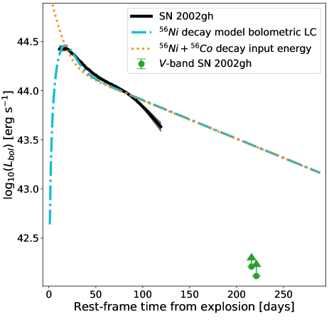
Figure 13: Fit of the radioactive decay of ⁵⁶Ni (Eq. 7) to the bolometric light curve of SN 2002gh, using the Arnett (1982) analytic approximation. The parameters of the best fit model are $\tau_{\mathrm{rise}}=17.3$ days, $M_{\mathrm{ej}}=0.9M_{\sun}$, $M_{\mathrm{Ni}}=13.6M_{\sun}$, $v_{\mathrm{ej}}=10,000$ km s^-1 and $\kappa=0.2$ cm² gr^-1. This model illustrates that the light curve of SN 2002gh follows an evolution “consistent” with the ⁵⁶Ni decay until about 70-80 days post maximum. However, the best fit obtained with the ⁵⁶Ni decay model is non-physical as $M_{\mathrm{Ni}}\textgreater M_{\mathrm{ej}}$, thus we can rule out the ⁵⁶Ni decay as the main power source for SN 2002gh.

3.5.3 Circumstellar medium interaction

An alternative scenario to explain the observed luminosities of SLSNe is the interaction between the SN ejecta an a massive CSM (see Moriya et al., 2018, and references therein). The smoking gun evidence for ejecta-CSM interaction in SLSNe-I is the presence of broad hydrogen or helium emission lines (see e.g., Yan et al., 2015, 2017; Fiore et al., 2021; Pursiainen et al., 2022). Alternatively, a bumpy structure in the SN light curve could be a signature of CSM interaction as well (see e.g., Yan et al., 2017; Fiore et al., 2021).

In the case of SN 2002gh we do not find clear signatures of ejecta-CSM interaction. In particular, the spectra of SN 2002gh do not show any signature of interaction (see Section 3.1). Inspecting carefully the early $I-$band bumpy structure (Section 3.3), we find that the residuals between the photometric observations and the light curve interpolation are correlated with the photometric uncertainty. No correlation is found between the $I-$band residuals and the residuals in the other bands as would be expected for the case of CSM interaction. The $B$ and $V$ light curves show a smooth evolution, without signatures of bumps.

The potential signatures of ejecta-CSM interaction are the break in the $BVI$ light curves at about 70 days after maximum light and the light curve flattening at late times. The light curve break does not exhibit an increase in the SN luminosity as is usually observed in bumps produced by the ejecta-CSM interaction (see Yan et al., 2017; Fiore et al., 2021). In SN 2002gh the break consists in an increase of the decline rates in all bands (see Section 3.3), potentially explained by the leakage of high-energy radiation (see Section 3.5.1; Wang et al., 2015; Vurm & Metzger, 2021). Unfortunately, we do not have a spectrum of SN 2002gh at the time of the break or at the time of the flattening to detect spectral features associated with a potential ejecta-CSM late time interaction.

4 Discussion and conclusions

We have presented and analysed excellent quality observations of SN 2002gh obtained as part of the CATS project. SN 2002gh is at a redshift of $z=0.365\pm 0.001$, it was the second SLSN-I discovered after SN 1999as, and its true nature remained unnoticed for two decades. The multi-band observations presented here for SN 2002gh cover 210 days in the rest-frame of the SN evolution, with a well sampled spectral sequence comprising 60 days. These observations make of SN 2002gh a perfect object for a detailed study, such as the one presented here.

In Section 3.1 we study the spectral evolution of SN 2002gh, identifying several ions at an expansion velocity decreasing from $11,000$ in the early phase to $9000$ km s^-1 in the later phases. We compare the spectra of SN 2002gh with well observed hydrogen-poor SLSNe and stripped envelope core-collapse SNe from the literature. The spectral evolution of SN 2002gh is typical of an object of this class displaying O ii lines before and close to maximum light, following a cooling phase, where the Fe ii lines become prominent features. After about +26 days the SN starts to resemble to Type Ic SN 1994I or to Type Ic-BL SN 2002ap at an early phase. SN 2002gh shows significant spectroscopic similarity to iPTF13ajg, which is also a bright object of this SN class (Vreeswijk et al., 2014).

In Section 3.2 we identified the potential SN 2002gh’s host galaxy in deep DECam images. The potential host is a faint dwarf galaxy, presumably having low metallicity as is common for a SLSN-I hosts (Lunnan et al., 2014; Leloudas et al., 2015; Perley et al., 2016; Schulze et al., 2018), located 0$\aas@@fstack{\prime\prime}$13 south-east from the SN location corresponding to a projected distance of 0.67 kpc, at the SN redshift. The host galaxy candidate shows irregular morphology and multiple emission peaks. The multi-peak morphology could be tracing regions of strong star-formation within the irregular host or could be interpreted as a system of dwarf galaxies in a merging process. Recently, Ørum et al. (2020) found that hydrogen-poor SLSN host galaxies are often part of interacting systems, with $\sim 50$% having at least one major companion within 5 kpc. They interpreted this as SLSNe-I being the result of a recent burst of star formation, possibly triggered by galaxy interaction. Future confirmation that the SN 2002gh’s host galaxy is part of a system of dwarf galaxies in a merging process, would provide further support to the Ørum et al. (2020) hypothesis. Further deep spectroscopy of the host galaxy candidate is required for a solid association with the SN and to understand the nature of the multi-peak morphology.

In Sections 3.3 and 3.4 we characterized the light curves of SN 2002gh and computed its bolometric light curve assuming that the SN emission can be well described by a modified blackbody. We distinguished four phases in the light curves of SN 2002gh. The first phase associated with the maximum light and the immediate decline from maximum, a second phase from about two weeks to $\simeq+70$ days post maximum, which is characterized by a bolometric decline rate roughly consistent with the decline rate expected for a SN powered by ⁵⁶Co decay. A third phase, from about $+70$ days to $\simeq 100$ days, characterized by a faster decline rate in all bands. The last phase comprises the last three photometric observations in the $V$-band, with a gap of nearly a hundred days between the first and the last two points. We find that the average decline rate value over this phase is reduced compared to the decline rate of the previous phase, indicating a possible flattening of the light curve at about 200 days after maximum.

In Section 3.4 we find that the maximum bolometric luminosity of SN 2002gh is $2.6\pm 0.1\times 10^{44}$ erg s^-1 ($log_{10}(L^{\mathrm{peak}}_{\mathrm{bol}})\simeq 44.4$). Our study presents a large set of bolometric light curves for 28 SLSNe-I, 11 from Pan-STARRS1 (Lunnan et al., 2018) and 17 from DES (Angus et al., 2019), showing the large diversity in shapes, including the presence of pre- and post-maximum bumps, and a large range in maximum luminosities from $log_{10}(L_{\mathrm{bol}})\simeq 43.2$ to $log_{10}(L_{\mathrm{bol}})<44.6$. A comparison of the bolometric light curve of SN 2002gh with these objects shows that SN 2002gh is the brightest in this sample. Comparing the estimated maximum bolometric luminosity for a total sample of 37 SLSNe-I, 16 from Pan-STARRS1 and 21 from DES, we show that SN 2002gh is among the most luminous SNe ever observed.

In Section 3.5 we study the magnetar model and the radioactive decay of ⁵⁶Ni as power sources of SN 2002gh. We rule out the radioactive decay of ⁵⁶Ni as the main power source for the light curve of SN 2002gh, finding that a minimum of $\simeq 13M_{\sun}$ of ⁵⁶Ni are needed to power the peak luminosity of SN 2002gh, an unrealistically large value. Moreover, the best analytic fitting to the bolometric light curve always requires a total ejecta mass below the ⁵⁶Ni mass, which is a non-physical solution, thus ruling out the radioactive decay of ⁵⁶Ni as the main power source for SN 2002gh. Although some amount of ⁵⁶Ni must be synthesized during the SN explosion.

We found that the spin down of a magnetar can explain the huge maximum luminosity observed in SN 2002gh. Fitting an analytic magnetar model to the observed bolometric light curve of SN 2002gh we found two alternative solutions. The first solution, requires significant leakage of the magnetar input energy (see Fig. 12), of which the rapid decline observed in the third phase of the SN light curves could be a signature. We found that the best fit to the bolometric light curve is for $M_{\mathrm{ej}}$ between 0.6 and 3.2 $M_{\sun}$, $P_{\mathrm{spin}}=3.2$ ms, and $B=5\times 10^{13}$ G. The alternative magnetar model does not require power leakage, and it is characterized by a huge ejecta mass of 25 to 40 $M_{\sun}$, a fast spin period of $P_{\mathrm{spin}}$ between 0.6 and 1.2 ms, and $B$ between 1.6 and 2.0$\times 10^{14}$ G.

SN 2002gh lacks signatures of hydrogen or helium mixed in the SN ejecta, therefore it must have lost all its hydrogen and a significant part of its helium envelope through winds, but also through binary interaction, since half or more of all massive stars are found in binary systems. Using equations 13 and 14 of Woosley (2019) for evolution models of massive helium stars in binary systems of solar metallicity, and assuming a final mass ($M_{\mathrm{fin}}$) before the explosion between 2.3 and 4.9 $M_{\sun}$ and of about 30 $M_{\sun}$ for the first and second case of the magnetar model, respectively. We estimate a zero-age main-sequence mass between 14 and 25 $M_{\sun}$ for the first case and of about 135 $M_{\sun}$ for the second case. These estimates for the main-sequence masses are particularly uncertain at very high mass, due to the uncertainty in the mass loss prescription (see Woosley, 2019), and the sensitivity of the mass loss to metallicity. Although we provide just a crude mass estimate for the second case, this estimate would place the progenitor star of SN 2002gh among the most massive stars observed to explode as a SN.

We do not find evidence that the ejecta-CSM interaction is the power source of the maximum luminosity of SN 2002gh, although late time interaction cannot be discounted (see Section 3.5.3). The spectral features of SN 2002gh are typical of a non-interacting SN, resembling non-interacting stripped envelope core-collapse SNe from about +24 days to the last spectrum at about +54 days (see Fig. 6) relative to the bolometric maximum. However, we cannot rule out completely the case of ejecta-CSM interaction in SN 2002gh, but we can place some constraints on the potential CSM composition, such as the CSM must be hydrogen and helium poor. We also note that the magnetar model can explain reasonably well the observations of SN 2002gh without the need to invoke the additional power contribution from the ejecta-CSM interaction.

Data Availability

The photometric data of SN 20202gh is available in the article and the spectra are available on request to the corresponding author and also available from the WISeREP archive (Yaron & Gal-Yam, 2012).

Appendix A Bolometric light curves

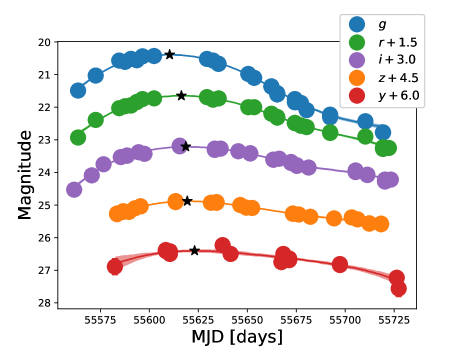
Figure 14: Gaussian process light curve interpolation for PS1-11ap. Continous lines correspond to the light curve interpolation and shaded regions to 1 $\sigma$ uncertainties. Black stars mark the peak brightness for each filter.

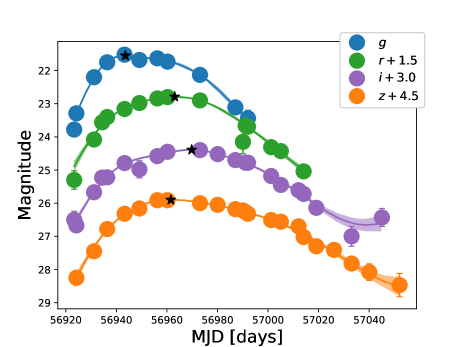
Figure 15: Gaussian process light curve interpolation for DES14X2byo. Continous lines correspond to the light curve interpolation and shaded regions to 1 $\sigma$ uncertainties. Black stars mark the peak brightness for each filter.

We constructed bolometric light curves from Pan-STARRS1 (PS1; Lunnan et al., 2018) and DES (Angus et al., 2019) SLSNe following a procedure identical to the one used for SN 2002gh. First we interpolated their light curves using the python Gaussian process module implemented in scikit-learn (Pedregosa et al., 2011), using the RBF and Matern kernels. The PS1 dataset is composed of observations in $grizy$ reaching a depth slightly fainter than $\sim 23.3$ mag in $griz$ and $\sim 22$ in $y-$band. Only a handful of objects have $y-$band photometry, usually more noisy than on the other filters. DES present a homogeneous set of photometry in $griz$ passbands to a depth of $\sim 24$ mag, obtained with the Dark Energy Camera (Flaugher et al., 2015) which is mounted on the 4 meter Blanco telescope at Cerro Tololo in Chile. In figures 14 and 15 we present two examples of the light curves interpolation, for PS1-11ap (Fig. 14) and for DES14X2byo (Fig. 15). One of the advantages of using Gaussian process interpolation is its flexibility, providing an excellent fit to the SLSNe light curves, as can be observed in these examples. At the same time, this approach provides a robust estimate for the uncertainty in the interpolation. Using this approach we obtained an homogeneous set of 37 multi-band interpolated light curves with their respective uncertainties, the latter point is key for the determination of the uncertainties in blackbody parameters and in our bolometric light curves.

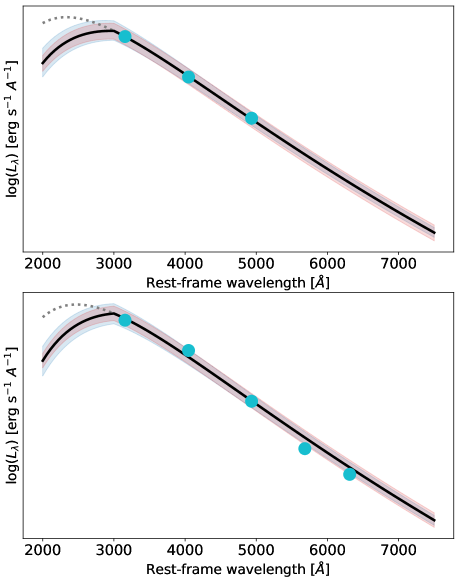
Figure 16: Blackbody fits to the interpolated photometry of PS1-11ap at -22.5 days relative to bolometric maximum (top) and at bolometric maximum (bottom). The solid line is the modified blackbody SED with a linear flux suppression below the “cutoff” wavelength at 3000 Å. The dotted line shows the full blackbody for comparison. Shaded blue regions correspond to 1 sigma uncertainty in $T_{bb}$ ($R_{bb}$ fixed) and shaded red regions correspond to 1 sigma uncertainty in $R_{bb}$ ($T_{bb}$ fixed).

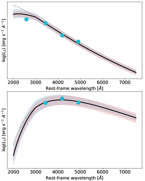
Figure 17: Blackbody fits to the interpolated photometry of DESX214byo at bolometric maximum (top) and at +22.5 relative to bolometric maximum (bottom). The solid line is the modified blackbody SED with a linear flux suppression below the “cutoff” wavelength at 3000 Å. The dotted line shows the full blackbody for comparison. Shaded blue regions correspond to 1 sigma uncertainty in $T_{bb}$ and shaded red regions correspond to 1 sigma uncertainty in $R_{bb}$.

To model the SLSN emission we fitted the interpolated light curves corrected for Galactic extinction using a modified blackbody SED. To correct the light curves by Galactic extinction we used $E(B-V)$ values from Schlafly & Finkbeiner (2011) and the Cardelli et al. (1989) reddening law with $R_{V}=3.1$, and no correction for host galaxy extinction was attempted. We converted magnitudes in the AB system to monochromatic fluxes following the Fukugita et al. (1996) definition (see also, e.g., Tonry et al., 2012). The effective wavelength and full-width at half maximum were computed for each filter using the DES and PS1 response functions, and we find good agreement with the values reported in Tonry et al. (2012) for PS1. The modified blackbody SED corresponds to the Planck function multiplied by a linear flux suppression below the “cutoff” wavelength at 3000 Å as shown in figures 16 and 17, where the linear flux suppression corresponds to a value between zero and one, with a value of zero at zero wavelength and one at 3000 Å. A similar modified SED has been repeatedly used in the literature (see e.g., Quimby et al., 2013; Nicholl et al., 2017). Despite the fact that the linear flux suppression below 3000 Å brings the blackbody emission in better agreement with photometric and spectroscopic observations of SLSNe (see Nicholl et al., 2017), the UV-region is dominated by broad absorption lines that are far from being a perfect modified blackbody. The deviation from this modified blackbody SED is expected to be larger in the UV region than in the optical, since at optical wavelengths broad absorption lines are shallow and the continuum dominates the SN emission until a few days or weeks after maximum. Thus, the rest-frame optical and NIR emission provides a better region to fit the underlying blackbody emission. As our bolometric light curves are based on a robust determination of the blackbody parameters ($T_{bb}$ and $R_{bb}$), we place the followinng requirements: 1) we only include SLSNe with $z$<1.2 in order to have at least one band, usually the $z$-band, located at a rest-frame wavelength greater than 4000 Å, where the ‘blackbody continuum’ is well defined in SLSNe and 2) the rest-frame effective wavelength of a band must be greater than 2900 Å to be considered in the fit. To fit a modified blackbody SED a minimum of two photometric bands is sufficient, but we generally required photometry in at least three bands. Only in cases where the blackbody fits with two photometric points shows a consistent evolution with blackbody fits obtained using more bands at adjacent epochs, we keep them. We noticed that this is usually the case for fits perfomed at a phase of before or close to maximum light, when the SLSN emission is very similar to a blackbody, and two photometric points with wavelength greater than $\sim 3500$ Å can constrain very well the blackbody parameters. This is no longer true at late times, a few weeks after maximum, when the SLSN emission deviates from a blackbody and two photometric points are not able to constrain the underlying pseudo-continuum. In these cases the fits are disregarded, sometimes even using three photometric observations we obtain fits that are not good and coherent with SED fits at previous epochs, in these cases the blackbody fits are disregarded as well.

To estimate the uncertainty in the fitted blackbody parameters a similar procedure as for SN 2002gh is followed. A new set of $15,000$ photometric observations is simulated assuming a Gaussian distribution with the standard deviation equal to the photometric uncertainty estimated using Gaussian process interpolation, and the blackbody parameters are re-computed obtaining a distribution for each of them. From the distribution obtained the uncertainties for $T_{bb}$ and $R_{bb}$ are estimated, computing lower and upper 1 $\sigma$ limits. Then, the bolometric emission using a blackbody SED with flux suppression below the “cutoff” wavelength is computed, and its corresponding 1 $\sigma$ uncertainty estimated.

In addition to the bolometric light curves, observed luminosity ($L_{\mathrm{obs}}$) light curves were constructed. To construct these light curves we summed the detected emission in the optical bands using our light curve interpolation method. When constructing these observed luminosity light curves care was put to take into account the effect of redshift in the effective wavelength and the width of the PS1 and DES filters. In tables 9 and 10 we summarize the maxima of the observed luminosity light curves.

In Fig. 18 the ratio between maximum $L_{\mathrm{bol}}$ and the maximum $L_{\mathrm{obs}}$ are presented. We find that the majority of the objects have a $L_{\mathrm{bol}}/L_{\mathrm{obs}}$ value between 1.5 and 3.5, with a mean value between 2.0 and 2.5. We computed the unweighted mean for $L_{\mathrm{bol}}/L_{\mathrm{obs}}$ for the redshift intervals $0.2\textless z\textless 0.6$, $0.6\leq z\leq 0.9$ and $0.9\textless z\textless 1.21$, obtaining the following values $2.2\pm 0.4$, $2.1\pm 0.5$ and $2.6\pm 0.6$, respectively. The weighted mean gives very similar values. The mean values for the PS1 sample are $2.1\pm 0.6$, $2.77\pm 0.03$ and $2.6\pm 0.5$ for the same redshift intervals, respectively and for the DES objects are $2.2\pm 0.2$, $1.9\pm 0.3$, and $2.6\pm 0.6$ for the same intervals, respectively. We notice that the most discrepant points are the ones with larger uncertainties, and that $L_{\mathrm{bol}}/L_{\mathrm{obs}}$ for SN 2002gh is $2.3\pm 0.1$ at $z=0.365$ (we do not include SN 2002gh in the computation).

To extend this relation beyond $z=1.2$ we used the well-observed DES16C2nm, which is a SLSN-I at $z=1.998$ (Smith et al., 2018). In their study, Smith et al. (2018) presents optical and NIR photometry and spectroscopy, showing that DES16C2nm is spectroscopically similar to iPTF13ajg. Unfortunately, the DES16C2nm NIR photometry covering the rest-frame optical continuum ($\lambda_{\mathrm{rest-frame}}\textgreater 3100$ Å) begins after maximum, therefore in order to estimate the maximum of the bolometric emission of DES16C2nm we constructed spectrophotometric templates. To construct these templates we used the spectroscopic observations of DES16C2nm and iPTF13ajg, which were binned, smoothed and joined, and then we scaled them using the $riz$ photometry for DES16C2nm. The DES16C2nm spectra were mangled, but did not mangled the iPTF13ajg spectra. The iPTF13ajg spectra were firstly scaled to join to the rest-frame UV of the mangled spectra of DES16C2nm, and then the combined spectral template was re-scaled using the $iz$ photometry. The early spectra of iPTF13ajg were scaled directly as no spectroscopic observations of DES16C2nm exists at an early phase. Then, we fitted a modified blackbody model to the spectrophotometric templates estimating the epoch maximum bolometric luminosity on $MJD=57684.0$, and the maximum luminosity $L_{\mathrm{bol}}=2.0\pm 0.2\times 10^{44}$ erg s^-1. Significant uncertanties are associated with these values due to the time gaps between the spectrophotometric templates and the potential systematic differences between DES16C2nm and iPTF13ajg, in additon to any other calibration issues. Therefore conservatively we quote $2.0\pm 0.4\times 10^{44}$ erg s^-1 as the estimated maximum bolometric luminosity for DES16C2nm in Table 10. Accordingly, we have extended the $L_{\mathrm{bol}}/L_{\mathrm{obs}}$ ratio to $z\simeq 2$, with $L_{\mathrm{bol}}/L_{\mathrm{obs}}=3.5\pm 0.7$ for DES16C2nm (see Fig. 18).

Having in mind that the rest-frame wavelength and the width of the wavelength range observed in the optical bands changes dramatically over the redshift range of our sample, we assume that this heuristic relation holds beyond $z\simeq 1.2$ and can be used to estimate the bolometric luminosity of PS1 and DES SLSNe with $z\textgreater 1.2$. For $z\textgreater 1.2$, we assume a $L_{\mathrm{bol}}/L_{\mathrm{obs}}$ ratio of 3.0, and we set the uncertainty of the $L_{\mathrm{bol}}/L_{\mathrm{obs}}$ ratio to 0.6. Then, we compute the $L_{\mathrm{bol}}$ uncertaninty as $\sqrt{(0.6\times L_{\mathrm{obs}})^{2}+(3.0\times\sigma_{L_{\mathrm{obs}}})^{2}}$.

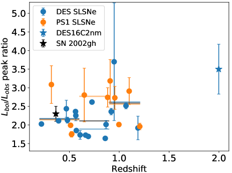
Figure 18: Ratio between the maximum bolometric luminosity and the maximum observed peak luminosity ($L_{\mathrm{bol}}/L_{\mathrm{obs}}$) as a function of redshift. We computed the unweighted mean for $L_{\mathrm{bol}}/L_{\mathrm{obs}}$ for the redshift intervals $0.2\textless z\textless 0.6$, $0.6\leq z\leq 0.9$ and $0.9\textless z\textless 1.21$, obtaining the following values $2.2\pm 0.4$, $2.1\pm 0.5$ and $2.6\pm 0.6$, respectively. The mean for the $L_{\mathrm{bol}}/L_{\mathrm{obs}}$ ratios are shown as grey horizontal lines for each redshift interval. The mean for PS1 and DES objects are shown as orange and blue horizontal lines for the same intervals, respectively. We show the location of SN 2002gh and DES16C2nm in this plot with black and blue stars, respectively. SN 2002gh was not included in the mean computation.

Table 9: Peak bolometric and peak observed luminosities for PS1 SLSNe.

SN	MJD peak $L_{bol}$	Peak $L_{bol}$	$T_{bb}$ at peak	$R_{bb}$ at peak	MJD peak $L_{obs}$	Peak $L_{obs}$	Redshift	$E(B-V)_{\mathrm{gal}}$
	(days)	($\times 10^{44}$ erg s)	($\times 10^{3}$ K)	($\times 10^{15}$ cm)		($\times 10^{43}$ erg s)
PS1-10ahf	55484.4	0.59(0.07)	$8.7^{+0.9}_{-0.7}$	$3.9^{+1.0}_{-0.8}$	55481.35	2.0(0.1)	1.10	0.0293
PS1-10awh	55497.3	2.8(0.5)	$34.8^{+10.2}_{-5.7}$	$0.8^{+0.2}_{-0.2}$	55504.8	8.1(0.2)	0.909	0.0658
PS1-10bzj	55544.9	1.4(0.3)	$28.9^{+12.2}_{-5.9}$	$0.8^{+0.2}_{-0.2}$	55559.9	4.9(0.1)	0.650	0.0068
PS1-10ky	55398.4	2.4(0.3)	$22.6^{+2.9}_{-2.2}$	$1.5^{+0.2}_{-0.2}$	55408.1	8.9(0.2)	0.956	0.0299
PS1-10pm	55334.1	1.17(0.04)	$11.2^{+0.7}_{-0.6}$	$3.4^{+0.4}_{-0.4}$	55323.6	5.9(0.2)	1.206	0.0153
PS1-11afv	–	2.0(0.4)‡	–	–	55731.4	6.6(0.4)	1.407	0.0138
PS1-11aib	55848.1	1.52(0.04)	$15.4^{+0.6}_{-0.5}$	$2.2^{+0.1}_{-0.1}$	55848.1	7.6(0.1)	0.997	0.0428
PS1-11ap	55612.6	1.42(0.03)	$11.7^{+0.3}_{-0.3}$	$3.4^{+0.1}_{-0.1}$	55612.6	8.0(0.1)	0.524	0.0059
PS1-11bam	–	3.2(0.6)‡	–	–	55889.1	10.7(0.4)	1.565	0.0234
PS1-11tt	–	1.4(0.3)‡	–	–	55710.6	4.5(0.2)	1.283	0.0080
PS1-12bmy	–	1.5(0.3)‡	–	–	56206.0	4.9(0.2)	1.572	0.0091
PS1-12bqf	56240.1	0.44(0.01)	$11.6^{+0.6}_{-0.6}$	$1.9^{+0.2}_{-0.1}$	56244.6	2.5(0.1)	0.522	0.0242
PS1-12cil	56291.1	0.9(0.1)	$19.2^{+3.4}_{-1.4}$	$1.2^{+0.1}_{-0.2}$	56303.1	2.9(0.1)	0.32	0.0234
PS1-13gt	56326.6	0.62(0.05)	$7.1^{+0.4}_{-0.3}$	$5.9^{+0.9}_{-0.8}$	56331.1	2.3(0.1)	0.884	0.0152
PS1-13or	–	3.8(0.8)‡	–	–	56393.1	12.6(0.2)	1.52	0.0308
PS1-14bj	56802.4	0.389(0.004)	$7.4^{+0.1}_{-0.1}$	$4.2^{+0.1}_{-0.1}$	56802.4	1.9(0.1)	0.5125	0.0189

• Numbers in parentheses correspond to 1 $\sigma$ statistical uncertainties. ^‡Maximum bolometric luminosities estimated scaling the observed maximum luminosities.

Table 10: Peak bolometric and peak observed luminosities for DES SLSNe.

SN	MJD peak $L_{bol}$	Peak $L_{bol}$	$T_{bb}$ at peak	$R_{bb}$ at peak	MJD peak $L_{obs}$	Peak $L_{obs}$	Redshift	$E(B-V)_{\mathrm{gal}}$
	(days)	($\times 10^{44}$ erg s)	($\times 10^{3}$ K)	($\times 10^{15}$ cm)		($\times 10^{43}$ erg s)
DES13S2cmm	56567.3	0.242(0.004)	$9.5^{+0.2}_{-0.2}$	$2.1^{+0.1}_{-0.1}$	56565.8	1.40(0.02)	0.663	0.0284
DES14C1fi	–	2.2(0.4)‡	–	–	56930.9	7.25(0.07)	1.302	0.0091
DES14C1rhg	57008.8	0.196(0.001)	$15.3^{+0.6}_{-0.5}$	$0.78^{+0.04}_{-0.04}$	57013.3	0.92(0.01)	0.481	0.0096
DES14E2slp	57041.1	0.48(0.01)	$13.1^{+0.3}_{-0.3}$	$1.61^{+0.06}_{-0.06}$	57042.6	2.58(0.04)	0.57	0.0060
DES14S2qri	–	1.8(0.4)‡	–	–	57022.7	5.9(0.2)	1.50	0.0276
DES14X2byo	56962.3	1.54(0.08)	$16.6^{+0.9}_{-0.8}$	$1.9^{+0.1}_{-0.1}$	56959.3	7.63(0.07)	0.868	0.0257
DES14X3taz	57082.6	1.28(0.06)	$11.5^{+0.9}_{-0.7}$	$3.4^{+0.5}_{-0.4}$	57082.6	7.4(0.4)	0.608	0.0220
DES15C3hav	57337.9	0.209(0.006)	$13.4^{+0.4}_{-0.3}$	$1.03^{+0.03}_{-0.03}$	57340.9	0.99(0.01)	0.392	0.0077
DES15E2mlf	–	3.1(0.6)‡	–	–	57358.0	10.2(0.4)	1.861	0.0086
DES15S1nog	57371.7	0.42(0.02)	$17.9^{+1.0}_{-0.8}$	$0.88^{+0.05}_{-0.05}$	57379.2	1.87(0.03)	0.565	0.0541
DES15S2nr	57316.8	0.441(0.005)	$10.5^{+0.1}_{-0.1}$	$2.32^{+0.04}_{-0.04}$	57321.3	2.18(0.01)	0.220	0.0293
DES15X1noe	57450.7	1.5(0.2)	$12.6^{+3.3}_{-2.0}$	$3.1^{+1.1}_{-0.9}$	57426.7	7.8(0.3)	1.188	0.0177
DES15X3hm	57239.9	1.55(0.02)	$13.9^{+0.4}_{-0.4}$	$2.6^{+0.1}_{-0.1}$	57235.4	9.46(0.09)	0.86	0.0237
DES16C2aix	57706.9	0.47(0.01)	$8.4^{+0.3}_{-0.3}$	$3.7^{+0.3}_{-0.3}$	57706.9	1.88(0.04)	1.068	0.0114
DES16C2nm	57684.0	2.0(0.40)†	$13.1^{+0.8}_{-0.8}$	$3.5^{+0.3}_{-0.3}$	57632.4	5.96(0.02)	1.998	0.0123
DES16C3cv	57769.9	0.264(0.003)	$6.2^{+0.1}_{-0.1}$	$5.0^{+0.1}_{-0.1}$	57772.9	1.01(0.01)	0.727	0.0103
DES16C3dmp	57723.2	0.65(0.01)	$18.8^{+0.4}_{-0.4}$	$1.00^{+0.02}_{-0.02}$	57726.2	2.76(0.02)	0.562	0.0068
DES16C3ggu	57791.6	1.7(0.7)	$29.9^{+12.7}_{-6.4}$	$0.8^{+0.2}_{-0.2}$	57800.6	4.71(0.06)	0.949	0.0074
DES17C3gyp	58152.1	1.78(0.02)	$14.9^{+1.2}_{-0.9}$	$2.5^{+0.2}_{-0.2}$	58144.6	7.3(0.2)	0.47	0.0073
DES17X1amf	58063.9	1.8(0.2)	$18.0^{+0.7}_{-0.6}$	$1.82^{+0.09}_{-0.09}$	58066.9	7.92(0.07)	0.92	0.0207
DES17X1blv	58068.2	0.273(0.006)	$10.6^{+0.4}_{-0.3}$	$1.8^{+0.2}_{-0.2}$	58068.2	1.61(0.03)	0.69	0.0213

• Numbers in parentheses correspond to 1 $\sigma$ statistical uncertainties. ^†Maximum bolometric luminosity estimated using spectrophotometric templates. ^‡Maximum bolometric luminosities estimated scaling the observed maximum luminosities.

References

- Aldering et al. (2002) Aldering G., et al., 2002, in Tyson J. A., Wolff S., eds, Society of Photo-Optical Instrumentation Engineers (SPIE) Conference Series Vol. 4836, Survey and Other Telescope Technologies and Discoveries. pp 61–72, doi:10.1117/12.458107
- Amorín et al. (2014) Amorín R., et al., 2014, A&A, 568, L8
- Amorín et al. (2015) Amorín R., et al., 2015, A&A, 578, A105
- Anderson et al. (2018) Anderson J. P., et al., 2018, A&A, 620, A67
- Angus et al. (2016) Angus C. R., Levan A. J., Perley D. A., Tanvir N. R., Lyman J. D., Stanway E. R., Fruchter A. S., 2016, MNRAS, 458, 84
- Angus et al. (2019) Angus C. R., et al., 2019, MNRAS, 487, 2215
- Antoniadis et al. (2016) Antoniadis J., Tauris T. M., Ozel F., Barr E., Champion D. J., Freire P. C. C., 2016, arXiv e-prints, p. arXiv:1605.01665
- Arnett (1982) Arnett W. D., 1982, ApJ, 253, 785
- Atek et al. (2011) Atek H., et al., 2011, ApJ, 743, 121
- Barbary et al. (2009) Barbary K., et al., 2009, ApJ, 690, 1358
- Barkat et al. (1967) Barkat Z., Rakavy G., Sack N., 1967, Phys. Rev. Lett., 18, 379
- Bertin & Arnouts (1996) Bertin E., Arnouts S., 1996, A&AS, 117, 393
- Bertin et al. (2002) Bertin E., Mellier Y., Radovich M., Missonnier G., Didelon P., Morin B., 2002, in Bohlender D. A., Durand D., Handley T. H., eds, Astronomical Society of the Pacific Conference Series Vol. 281, Astronomical Data Analysis Software and Systems XI. p. 228
- Bessell (1990) Bessell M. S., 1990, PASP, 102, 1181
- Bessell (2005) Bessell M. S., 2005, ARA&A, 43, 293
- Bessell et al. (1998) Bessell M. S., Castelli F., Plez B., 1998, A&A, 333, 231
- Cardamone et al. (2009) Cardamone C., et al., 2009, MNRAS, 399, 1191
- Cardelli et al. (1989) Cardelli J. A., Clayton G. C., Mathis J. S., 1989, ApJ, 345, 245
- Cartier et al. (2014) Cartier R., et al., 2014, ApJ, 789, 89
- De Cia et al. (2018) De Cia A., et al., 2018, ApJ, 860, 100
- Dessart (2018) Dessart L., 2018, A&A, 610, L10
- Dessart (2019) Dessart L., 2019, A&A, 621, A141
- Dessart et al. (2012) Dessart L., Hillier D. J., Waldman R., Livne E., Blondin S., 2012, MNRAS, 426, L76
- Fiore et al. (2021) Fiore A., et al., 2021, MNRAS, 502, 2120
- Flaugher et al. (2015) Flaugher B., et al., 2015, AJ, 150, 150
- Fukugita et al. (1996) Fukugita M., Ichikawa T., Gunn J. E., Doi M., Shimasaku K., Schneider D. P., 1996, AJ, 111, 1748
- Gal-Yam (2019a) Gal-Yam A., 2019a, ARA&A, 57, 305
- Gal-Yam (2019b) Gal-Yam A., 2019b, ApJ, 882, 102
- Gal-Yam et al. (2009) Gal-Yam A., et al., 2009, Nature, 462, 624
- Gezari et al. (2009) Gezari S., et al., 2009, ApJ, 690, 1313
- Grayling et al. (2021) Grayling M., et al., 2021, arXiv e-prints, p. arXiv:2103.14669
- Guillochon et al. (2018) Guillochon J., Nicholl M., Villar V. A., Mockler B., Narayan G., Mandel K. S., Berger E., Williams P. K. G., 2018, ApJS, 236, 6
- Hamuy et al. (2003) Hamuy M., et al., 2003, Nature, 424, 651
- Hamuy et al. (2006) Hamuy M., et al., 2006, PASP, 118, 2
- Hamuy et al. (2009) Hamuy M., et al., 2009, ApJ, 703, 1612
- Hatano et al. (1999) Hatano K., Branch D., Fisher A., Millard J., Baron E., 1999, ApJS, 121, 233
- Heger & Woosley (2002) Heger A., Woosley S. E., 2002, ApJ, 567, 532
- Inserra et al. (2013) Inserra C., et al., 2013, ApJ, 770, 128
- Inserra et al. (2018) Inserra C., et al., 2018, MNRAS, 475, 1046
- Jerkstrand et al. (2016) Jerkstrand A., Smartt S. J., Heger A., 2016, MNRAS, 455, 3207
- Jerkstrand et al. (2017) Jerkstrand A., et al., 2017, ApJ, 835, 13
- Jerkstrand et al. (2020) Jerkstrand A., Maeda K., Kawabata K. S., 2020, Science, 367, 415
- Kasen & Bildsten (2010) Kasen D., Bildsten L., 2010, ApJ, 717, 245
- Knop et al. (1999) Knop R., et al., 1999, IAU Circ., 7128, 1
- Leloudas et al. (2015) Leloudas G., et al., 2015, MNRAS, 449, 917
- Liu et al. (2017) Liu Y.-Q., Modjaz M., Bianco F. B., 2017, ApJ, 845, 85
- Lunnan et al. (2014) Lunnan R., et al., 2014, ApJ, 787, 138
- Lunnan et al. (2015) Lunnan R., et al., 2015, ApJ, 804, 90
- Lunnan et al. (2018) Lunnan R., et al., 2018, ApJ, 852, 81
- Maeda et al. (2007) Maeda K., et al., 2007, ApJ, 666, 1069
- Mazzali et al. (2016) Mazzali P. A., Sullivan M., Pian E., Greiner J., Kann D. A., 2016, MNRAS, 458, 3455
- Mazzali et al. (2019) Mazzali P. A., Moriya T. J., Tanaka M., Woosley S. E., 2019, MNRAS, 484, 3451
- Milisavljevic et al. (2013) Milisavljevic D., et al., 2013, ApJ, 770, L38
- Miller et al. (2009) Miller A. A., et al., 2009, ApJ, 690, 1303
- Modjaz et al. (2014) Modjaz M., et al., 2014, AJ, 147, 99
- Moriya et al. (2018) Moriya T. J., Sorokina E. I., Chevalier R. A., 2018, Space Sci. Rev., 214, 59
- Nadyozhin (1994) Nadyozhin D. K., 1994, ApJS, 92, 527
- Neill et al. (2011) Neill J. D., et al., 2011, ApJ, 727, 15
- Nicholl et al. (2015) Nicholl M., et al., 2015, ApJ, 807, L18
- Nicholl et al. (2016a) Nicholl M., et al., 2016a, ApJ, 826, 39
- Nicholl et al. (2016b) Nicholl M., et al., 2016b, ApJ, 828, L18
- Nicholl et al. (2017) Nicholl M., Guillochon J., Berger E., 2017, ApJ, 850, 55
- Nicholl et al. (2019) Nicholl M., Berger E., Blanchard P. K., Gomez S., Chornock R., 2019, ApJ, 871, 102
- Ofek et al. (2007) Ofek E. O., et al., 2007, ApJ, 659, L13
- Ørum et al. (2020) Ørum S. V., Ivens D. L., Strandberg P., Leloudas G., Man A. W. S., Schulze S., 2020, A&A, 643, A47
- Pastorello et al. (2010) Pastorello A., et al., 2010, ApJ, 724, L16
- Pedregosa et al. (2011) Pedregosa F., et al., 2011, Journal of Machine Learning Research, 12, 2825
- Perley et al. (2016) Perley D. A., et al., 2016, ApJ, 830, 13
- Prajs et al. (2017) Prajs S., et al., 2017, MNRAS, 464, 3568
- Pursiainen et al. (2022) Pursiainen M., et al., 2022, arXiv e-prints, p. arXiv:2202.01635
- Quimby et al. (2007) Quimby R. M., Aldering G., Wheeler J. C., Höflich P., Akerlof C. W., Rykoff E. S., 2007, ApJ, 668, L99
- Quimby et al. (2011) Quimby R. M., et al., 2011, Nature, 474, 487
- Quimby et al. (2013) Quimby R. M., Yuan F., Akerlof C., Wheeler J. C., 2013, MNRAS, 431, 912
- Quimby et al. (2018) Quimby R. M., et al., 2018, ApJ, 855, 2
- Rakavy & Shaviv (1967) Rakavy G., Shaviv G., 1967, ApJ, 148, 803
- Schlafly & Finkbeiner (2011) Schlafly E. F., Finkbeiner D. P., 2011, ApJ, 737, 103
- Schlegel (1990) Schlegel E. M., 1990, MNRAS, 244, 269
- Schulze et al. (2018) Schulze S., et al., 2018, MNRAS, 473, 1258
- Smith et al. (2007) Smith N., et al., 2007, ApJ, 666, 1116
- Smith et al. (2016) Smith M., et al., 2016, ApJ, 818, L8
- Smith et al. (2018) Smith M., et al., 2018, ApJ, 854, 37
- Tonry et al. (2012) Tonry J. L., et al., 2012, ApJ, 750, 99
- Vreeswijk et al. (2014) Vreeswijk P. M., et al., 2014, ApJ, 797, 24
- Vurm & Metzger (2021) Vurm I., Metzger B. D., 2021, ApJ, 917, 77
- Wang et al. (2015) Wang S. Q., Wang L. J., Dai Z. G., Wu X. F., 2015, ApJ, 799, 107
- Wood-Vasey et al. (2002) Wood-Vasey W. M., Aldering G., Nugent P., Rudas R., 2002, IAU Circ., 7990
- Woosley (2010) Woosley S. E., 2010, ApJ, 719, L204
- Woosley (2019) Woosley S. E., 2019, ApJ, 878, 49
- Woosley et al. (2007) Woosley S. E., Blinnikov S., Heger A., 2007, Nature, 450, 390
- Yan et al. (2015) Yan L., et al., 2015, ApJ, 814, 108
- Yan et al. (2017) Yan L., et al., 2017, ApJ, 848, 6
- Yaron & Gal-Yam (2012) Yaron O., Gal-Yam A., 2012, PASP, 124, 668