Intersecting diametral balls induced by
a geometric graph

Abstract.

For a graph whose vertex set is a finite set of points in the Euclidean $d$-space consider the closed (open) balls with diameters induced by its edges. The graph is called a (an open) Tverberg graph if these closed (open) balls intersect. Using the idea of halving lines, we show that (i) for any finite set of points in the plane, there exists a Hamiltonian cycle that is a Tverberg graph; (ii) for any $n$ red and $n$ blue points in the plane, there exists a perfect red-blue matching that is a Tverberg graph. Also, we prove that (iii) for any even set of points in the Euclidean $d$-space, there exists a perfect matching that is an open Tverberg graph; (iv) for any $n$ red and $n$ blue points in the Euclidean $d$-space, there exists a perfect red-blue matching that is a Tverberg graph.

1. Introduction

Tverberg’s theorem is one of the essential results of modern discrete and convex geometry proved by Helge Tverberg [Tverberg1966] in 1966. It claims that for any set of $(r-1)(d+1)+1$ points in $\mathbb{R}^{d}$, there exists a partition with $r$ parts whose convex hulls intersect.

In the current paper, we consider a variation of Tverberg’s problem introduced recently in [bereg2019maximum, huemer2019matching, soberon2020tverberg]. For two points $x,y\in\mathbb{R}^{d}$, we denote by $B(xy)$ the closed Euclidean ball for which the segment $xy$ is its diameter. Let $G$ be a graph whose vertex set is a finite set of points in $\mathbb{R}^{d}$. We say that $G$ is a Tverberg graph if

$$\bigcap_{xy\in E(G)}B(xy)\neq\emptyset.$$

Replacing closed balls by open balls in the definition of Tverberg graph, we define an open Tverberg graph. A graph whose vertices are points in $\mathbb{R}^{d}$ is called an open Tverberg graph if the open balls with diameters induced by its edges intersect. Notice that there is a Tverberg graph which is not an open Tverberg graph, that is, the intersection of the closed balls induced by its edges is a single point lying on the boundary of some of them. For example, any Hamiltonian cycle for the set of vertices of a square is such a graph. For the sake of brevity, a perfect matching for an even set of points in $\mathbb{R}^{d}$ is called a (an open) Tverberg matching if it is a (an open) Tverberg graph. Analogously, a Hamiltonian cycle for a set of points in $\mathbb{R}^{d}$ is called a Tverberg cycle if it is a Tverberg graph.

In 2019, Huemer, Pérez-Lantero, Seara, and Silveira [huemer2019matching] showed that for any set of $n$ red points and $n$ blue points in the plane, there is a red-blue Tverberg matching (every edge connects points of different colors). This result can be considered as a colorful variation of the problem. Moreover, they proved that the matching maximizing the sum of the squared distances between the matched points is a Tverberg red-blue matching; see also Remark 15.

Later, Bereg, Chacón-Rivera, Flores-Peñaloza, Huemer, and Pérez-Lantero [bereg2019maximum] found a second proof of the monochromatic version of the result from [huemer2019matching], that is, for any $2n$ points in the plane, there is a Tverberg matching. Also, they showed that the matching maximizing the sum of the distances between the matched points is a desired matching.

Recently, Soberón and Tang [soberon2020tverberg] showed the existence of a Tverberg cycle for an odd set of points in the plane. As a corollary of this theorem, they proved that for any even set of points in the plane, there is a Hamiltonian path that is a Tverberg graph. Since a Hamitonian path for an even set of vertices contains a perfect matching, this corollary implies the result from [huemer2019matching]. Also, Soberón and Tang initiated the study of Tverberg graphs in higher dimensions, and in particular, they considered the problem of describing the family of Tverberg graphs for a finite set of points in $\mathbb{R}^{d}$; see Problem 1.1 in [soberon2020tverberg].

In 2007, twelve years before the paper [bereg2019maximum], Dumitrescu, Pach, and Tóth proved a lemma that is interesting in the context of Tverberg matchings; see Lemma 2 from [dumitrescu2009drawing]. This lemma easily implies that for any $2n$ distinct points in the plane, there exist a perfect matching $\mathcal{M}$ and a point $z$ in the plane such that either $z\in\{x,y\}$ or $\angle xzy\geq 2\pi/3$ for all $xy\in\mathcal{M}$. This result can be viewed as a strengthening of the existence of a Tverberg matching for an even set of points in the plane. Namely, this result claims that the common point of disks induced by the edges of the matching lies relatively deep inside of each disk. We refer to Subsection 9.2, where we discuss a higher-dimensional version of this problem.

The goal of the current paper is to show a variety of methods that can be useful in proving the existence of Tverberg cycles or matchings for point sets.

Using the idea of halving lines [lovasz1971number], we give short proofs of the following results.

Theorem 1.

For any finite set of points in the plane, there exists a Tverberg cycle.

Theorem 2.

For any set of $n$ red points and $n$ blue points in the plane, there exists a Tverberg red-blue matching.

Remark that Theorem 1 is a refinement of the main result from [soberon2020tverberg] mentioned earlier: Our approach also works for an even set of points in the plane. Theorem 2 is the main result from [huemer2019matching], however, we give a new proof which seems to be simpler than the original one. It is worth mentioning that our proofs of these theorems are very similar and this is not a coincidence because of the following connection between them. For any finite set of points in the plane, one can consider the colored multiset containing each point of the set colored in red and also a copy of each point colored in blue. Hence, in this setting, a Tverberg cycle can be viewed as a special red-blue Tverberg matching.

Our main results are higher-dimensional generalizations of the main theorem from [bereg2019maximum] and [huemer2019matching].

Theorem 3.

For any even set of distinct points in $\mathbb{R}^{d}$, there exists an open Tverberg matching.

Theorem 4.

For $n$ red points and $n$ blue points in $\mathbb{R}^{d}$, there exists a red-blue Tverberg matching.

Remark that Theorem 2 is a special case of Theorem 4. However, we decided to leave the proofs of both theorems because they are absolutely different. It is worth mentioning that Theorems 2 and 4 are in a sense tight: Consider the vertices of a square which are colored alternatively in red and blue; for any red-blue matching the intersection of the induced balls is a point.

Our proofs of Theorems 3 and 4 are based on the method of infinite descent. Note that both proofs of Tverberg’s theorem by Tverberg and Vrećica [Tverberg1993] and by Roudneff [Roudneff2001] give a good illustration of this method. Recalling that Tverberg’s theorem has a colorful variation (unfortunately, proved only in special cases; see [Barany1992, Blagojevi2015, Blagojevi2011]), we can also interpret Theorems 3 and 4 as a Tverberg-type theorem and its colorful version, respectively. Remark that the combinatorial and linear-algebraic ingredients of the proofs of Theorems 3 and 4 are different.

Throughout the paper, we use the standard notation of convex geometry and graph theory; see the books [barvinok2002course] and [west2001introduction] on convexity and graph theory, respectively.

The paper is organized as follows. In Section 2 we introduce the notation and discuss simple observations that we need to prove Theorems 1 and 2 in Sections 3 and 4, respectively. In Subsection 5.1, we study properties of the global minimum of a function playing the key role in the proofs of Theorems 3 and 4. In Subsection 5.2, we introduce a concept of obtuse graph and study its properties. Using the lemmas from Subsection 5.1 and 5.2, we prove Theorem 3 in Section 6. Finally, applying the lemma from Subsection 5.1, we give a proof of Theorem 4 in Section 7. In Section 8, we discuss the method of infinite descent in the context of Tverberg-type results. Finally, in Section 9, we propose a number of new open problems.

Acknowledgments.

We thank Pablo Soberón for sharing the problem. Besides, we thank János Pach for drawing our attention to [dumitrescu2009drawing]. We are also grateful to the members of the Laboratory of Combinatorial and Geometric Structures at MIPT for the stimulating and fruitful discussions. We thanks to the referees for their suggestions that helped us to significantly improve the presentation of the paper.

2. Preliminaries for planar results

We say that a finite set of points is in general position if no two segments spanned by points of the set are orthogonal or parallel.It is sufficient to prove Theorems 1 and 2 additionally assuming that the points are in general position. Indeed, for any $n$-tuple $S$ of points in the plane, consider a sequence $\{S_{k}\}_{k=1}^{\infty}$ of $n$-tuples of points in general position converging to $S$. Suppose that for each $S_{k}$, we can find a proper Tverberg graph, which naturally induces a graph $G_{k}$ with the vertex set $\{1,\dots,n\}$. Hence, there is a graph $G$ that occurs infinitely many times in the sequence $\{G_{k}\}_{k=1}^{\infty}$. Since there is a compactum containing all disks induces by pairs of points in $S$ or $S_{k}$, the corresponding graph for $S$ is also a Tverberg graph. Moreover, if each $G_{k}$ is a Hamiltonian cycle (or a perfect red-blue matching), so is the obtained graph. Throughout Sections 2, 3, and 4, we consider only finite point sets in general position in the plane.

For a finite non-empty set $S$ of points in the plane, a line is called bisecting if there are at most $|S|/2$ points of $S$ in each of its open half-planes.

Choose any unit vector $v$. Denote by $v_{\alpha}$ the unit vector obtained by the counterclockwise rotation of $v$ by an angle $\alpha$. Let $H_{\alpha}$ be the union of bisecting lines for $S$ orthogonal to $v_{\alpha}$. Therefore, $H_{\alpha}$ is a closed plank lying between two parallel bisecting lines, each of those passes through a point of $S$. Moreover, every line lying between the lines bounding $H_{\alpha}$ does not contain a point of $S$. Denote by $\ell_{\alpha}$ the midline of $H_{\alpha}$; see Figure 1(a). Since $H_{\alpha}=H_{\alpha+\pi}$, we obtain that the lines $\ell_{\alpha}$ and $\ell_{\alpha+\pi}$ coincide. For an odd set $S$, the plank $H_{\alpha}$ coincides with the line $\ell_{\alpha}$ passing through a point of $S$. For an even set $S$, the plank $H_{\alpha}$ coincides with the line $\ell_{\alpha}$ if and only if $\ell_{\alpha}$ passes through exactly two points of $S$. Denote by $\ell_{\alpha}^{+}$ the closed half-plane bounded by $\ell_{\alpha}$ such that $v_{\alpha}$ is its inner normal vector.

Lemma 5.

For any point of $S$, there is a bisecting line $\ell_{\alpha}$ passing through it.

Proof.

Consider any point $p$ in the plane and any bisecting line $\ell_{\beta}$. Suppose $p$ does not lie on $\ell_{\beta}$ and without loss of generality, assume that $p\in\ell_{\beta}^{+}$. Since the lines $\ell_{\beta}$ and $\ell_{\beta+\pi}$ coincide, we have $p\not\in\ell_{\beta+\pi}^{+}$. As $\ell_{\gamma}$ is the midline of $H_{\alpha}$, the half-plane $\ell_{\gamma}^{+}$ continuously depends on $\gamma$, and thus, there is $\alpha$ such that the point $p$ lies on $\ell_{\alpha}$. ∎

Corollary 6.

For an even set $S$ of points, there is a bisecting line $\ell_{\alpha}$ passing through two points of $S$.

Proof.

By Lemma 5, there is a bisecting line $\ell_{\alpha}$ passing through a point of $S$. Since $\ell_{\alpha}$ is the midline of $H_{\alpha}$, it coincides with $H_{\alpha}$, and hence, contains exactly two points of $S$. ∎

Denote by $o_{\alpha}$ the intersection point of lines $\ell_{\alpha}$ and $\ell_{\alpha+\pi/2}$. These lines determine four closed quadrants in the plane. Let us enumerate them in the counterclockwise order by $1,2,3,4$ starting from $\ell_{\alpha}^{+}\cap\ell_{\alpha+\pi/2}^{+}$; see Figures  2 and 3, where we denote the quadrants as $Q_{1},Q_{2},Q_{3},Q_{4}$, respectively. Remark that a point may belong to two distinct quadrants if and only if it lies on the intersection of their boundaries.

Corollary 7.

For an odd set $S$ of points, there are bisecting lines $\ell_{\alpha}$ and $\ell_{\alpha+\pi/2}$ such that each of them passes through exactly one of two distinct points of $S$.

Proof.

Consider two points $x,y\in S$ at the maximum distance among all pairwise distances between points of $S$. Clearly, both of them lie on the boundary of the convex hull of $S$. By Lemma 5, there is a bisecting line passing through the point $x$. If it contains two points of $S$, we may rotate it around $x$ a little bit in such a way that the resulting bisecting line $\ell_{\alpha}$ contains only the point $x$ of $S$. We claim that the line $\ell_{\alpha+\pi/2}$ does not pass through $x$. Indeed, suppose that $x=o_{\alpha}$. Without loss of generality, assume that $y$ lies in the second quadrant, and thus, there is a point $z\in S$ distinct from $x$ lying in fourth quadrant. Since $x$ is the closest point to $y$ in the fourth quadrant, we have $\|z-y\|>\|x-y\|$, a contradiction with maximality of the distance between $x$ and $y$, see Figure 1(b). Hence, the point $x$ does not lie on $\ell_{\alpha+\pi/2}$, and so, this line passes through another point of $S$. If it contains two points of $S$, then we may rotate $\ell_{\alpha}$ and $\ell_{\alpha+\pi/2}$ in such a way that each of them contains exactly one point of $S$. ∎

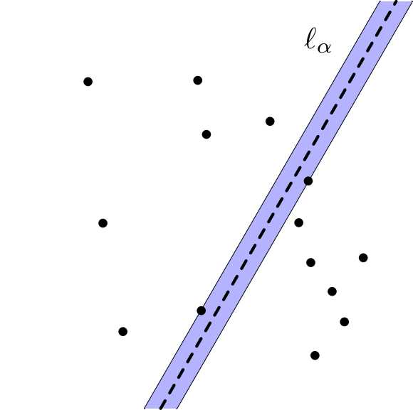
(a) Plank $H_{\alpha}$ and its midline $\ell_{\alpha}$.

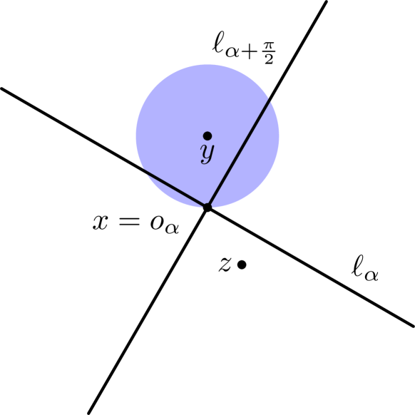
(b) Proof of Corollary 7.

Figure 1.

Next, we state a trivial observation playing the crucial role in proving Theorems 1 and 2.

Observation 8.

The point $o_{\alpha}$ lies in any disk with a diameter whose endpoints lie in two opposite quadrants.

3. Proof of Theorem 1

Let $S$ be a set of $n$ points in the plane. Consider two bisecting lines $\ell_{\alpha}$ and $\ell_{\alpha+\pi/2}$ orthogonal to each other. Later, we specify the choice of these lines. Denote by $s_{i}$ the number of points in the $i$-th closed quadrant.

There are several possible cases.

Figure 2. Case 1.1 ($n=8$), Case 1.2 ($n=8$), Case 2 ($n=9$).

Case 1. Let $n$ be even. By Corollary 6, we may choose a bisecting line $\ell_{\alpha}$ passing through exactly two points of $S$. Denote these points by $x$ and $y$. Since no two segments spanned by points of $S$ are orthogonal, the bisecting line $\ell_{\alpha+\pi/2}$ contains no points of $S$. There are two possible cases depending on the arrangement of the points $x,y,$ and $o_{\alpha}$ on the line $\ell_{\alpha}$.

Case 1.1. The point $o_{\alpha}$ lies between the points $x$ and $y$ on the line $\ell_{\alpha}$. Without loss of generality, assume that $x$ belongs to the second and third quadrants and the point $y$ belongs to the first and fourth quadrants. Since $\ell_{\alpha}$ and $\ell_{\alpha+\pi/2}$ are bisecting lines, we obtain that $s_{1}=s_{3}$ and $s_{2}=s_{4}$. Therefore, we easily construct a Hamiltonian cycle with edges satisfying Observation 8: We run alternatively between the points of the third and first quadrants starting from $x$ and finishing at $y$, and then we continue to run alternatively between the points of the fourth and second quadrants starting from $y$ and finishing at $x$.

Case 1.2. The points $x$ and $y$ lie on the same side with respect to $o_{\alpha}$ on the line $\ell_{\alpha}$. Without loss of generality assume that $x$ and $y$ belong to the first and fourth quadrants. Using the fact that $\ell_{\alpha}$ and $\ell_{\alpha+\pi/2}$ are bisecting lines, we obtain that $s_{1}=s_{3}+1$ and $s_{4}=s_{2}+1$. Therefore, we easily construct a Hamiltonian cycle with edges satisfying Observation 8: We run alternatively between the points of the first and third quadrants starting from $x$ and finishing at $y$, and then we continue to run alternatively between the points of the fourth and second quadrants starting from $y$ and finishing at $x$.

Case 2. Let $n$ be odd. By Corollary 7, we may choose bisecting lines $\ell_{\alpha}$ and $\ell_{\alpha+\pi/2}$ such that each of them passes through exactly one of two distinct points of $S$. Denote by $x$ the point of $S$ lying on $\ell_{\alpha}$ and by $y$ the point of $S$ lying on $\ell_{\alpha+\pi/2}$.

Without loss of generality, assume that the point $x$ belongs to the second and third quadrants and the point $y$ belongs to the first and second quadrants. Since $\ell_{\alpha}$ and $\ell_{\alpha+\pi/2}$ are bisecting lines, we obtain that $s_{1}=s_{3}$ and $s_{2}=s_{4}+1$. Therefore, we easily construct a Hamiltonian cycle with edges satisfying Observation 8: We run alternatively between the points of the third and first quadrants starting from $x$ and finishing at $y$, and then we continue to run alternatively between the points of the second and fourth quadrants starting from $y$ and finishing at $x$. $\square$

Remark 9.

Recently the following conjecture of Fekete and Woeginger [fekete1997angle] resembling Theorem 1 was confirmed by Biniaz [biniaz2021acute]: For any sufficiently large even number $n$, every set $S$ of $n$ points in the plane can be connected by a Hamiltonian cycle consisting of straight-line edges such that the angle between any two consecutive edges is at most $\pi/2$. As the first step of the proof he applied the idea from [dumitrescu2009drawing] similar to our approach. Namely, he considered two orthogonal bisecting lines for $S$ that partition the plane into four quadrants containing almost the same number of points in $S$ and used the following observation (compare with Observation 8): For any two distinct points $x,z$ lying in one quadrant and a point $y$ from the opposite quadrant, the angle $\angle xyz$ is acute. Also, note that the Tverberg cycle obtained in the proof of Theorem 1 contains a lot of acute angles, however, not necessarily all its angles are acute.

4. Proof of Theorem 2

Denote by $S$ the set of $n$ red points and $n$ blue points.

Figure 3. Illustrations showing that $|F(\alpha_{0}+\varepsilon)-F(\alpha_{0}-\varepsilon)|\leq 1$.

Using the notation of Section 2, consider a set $\Omega$ of $\alpha\in\mathbb{R}/2\pi\mathbb{Z}$ such that none of the bisecting lines $\ell_{\alpha}$ and $\ell_{\alpha+\pi/2}$ for $S$ passes through points of $S$. Remark that the complementary set $\overline{\Omega}=(\mathbb{R}/2\pi\mathbb{Z})\setminus\Omega$ is finite. Moreover, for every $\alpha\in\overline{\Omega}$, only one of two lines $\ell_{\alpha}$ or $\ell_{\alpha+\pi/2}$ passes through a point of $S$ (in fact, it passes through exactly two points of $S$).

For $\alpha\in\Omega$, denote the number of red and blue points in the $i$-th quadrant by $r_{i}(\alpha)$ and $b_{i}(\alpha)$, respectively. We claim that

$$r_{1}(\alpha)-b_{3}(\alpha)=r_{3}(\alpha)-b_{1}(\alpha)=b_{2}(\alpha)-r_{2}(\alpha)=b_{4}(\alpha)-r_{2}(\alpha).$$ (1)

Indeed, since the lines $\ell_{\alpha}$ and $\ell_{\alpha+\pi/2}$ are bisecting, we have $r_{1}(\alpha)+b_{1}(\alpha)=r_{3}(\alpha)+b_{3}(\alpha)$ and $r_{2}(\alpha)+b_{2}(\alpha)=r_{4}(\alpha)+b_{4}(\alpha)$. Consequently,

$$r_{1}(\alpha)-b_{3}(\alpha)=r_{3}(\alpha)-b_{1}(\alpha)\ \ \text{ and }\ \ b_{2}(\alpha)-r_{4}(\alpha)=b_{4}(\alpha)-r_{2}(\alpha).$$ (2)

Next, from the equality of the numbers of red and blue points we have

$$r_{1}(\alpha)+r_{2}(\alpha)+r_{3}(\alpha)+r_{4}(\alpha)=|S|/2=n=b_{1}(\alpha)+b_{2}(\alpha)+b_{3}(\alpha)+b_{4}(\alpha),$$

and thus,

$$\big{(}r_{1}(\alpha)-b_{3}(\alpha)\big{)}+\big{(}r_{3}(\alpha)-b_{1}(\alpha)\big{)}=\big{(}b_{2}(\alpha)-r_{4}(\alpha)\big{)}+\big{(}b_{4}(\alpha)-r_{2}(\alpha)\big{)}.$$

Combining this equality with (2), we easily obtain (1).

According to Observation 8, it is enough to prove that there is $\alpha\in\Omega$ such that the number of red points in any of quadrants equals to the number of blue points in its opposite quadrant. By (1), it remains to show that $r_{1}(\alpha)=b_{3}(\alpha)$ for some $\alpha\in\Omega$.

Finally, consider the function $F:\Omega\to\mathbb{Z}$ defined by $F(\alpha)=r_{1}(\alpha)-b_{3}(\alpha)$. Since $\ell_{\alpha}$ is a midline of $H_{\alpha}$, it changes continuously for $\alpha\in\mathbb{R}/2\pi\mathbb{Z}$, and thus, we get that $F$ is a piecewise constant function. Moreover, it is constant between any two consecutive points of $\overline{\Omega}$. We claim that $F$ changes its value at points of $\overline{\Omega}$ by 1, 0, or $-1$. Indeed, consider $\alpha_{0}\in\overline{\Omega}$. Let us change $\alpha$ continuously from $\alpha_{0}-\varepsilon$ to $\alpha_{0}+\varepsilon$, where $\varepsilon>0$ is chosen in such a way that $\alpha_{0}$ is the only point of $\overline{\Omega}$ lying between $\alpha_{0}-\varepsilon$ and $\alpha_{0}+\varepsilon$. We know that one of the lines $\ell_{\alpha_{0}}$ or $\ell_{\alpha_{0}+\pi/2}$ contains exactly two points of $S$ and the other does not pass through any point of $S$. Therefore, $|F(\alpha_{0}+\varepsilon)-F(\alpha_{0}-\varepsilon)|\leq 2$. Notice that $|F(\alpha_{0}+\varepsilon)-F(\alpha_{0}-\varepsilon)|$ can be equal to 2 only if one of the following properties holds for $\alpha=\alpha_{0}$: (i) the boundary of the first quadrant contains two red points; (ii) the boundary of the third quadrant contains two blue points; (iii) the boundary of the first quadrant contains one red point and the boundary of the third quadrant contains one blue point. There are 6 possible arrangements of these two points of $S$ and the point $o_{\alpha_{0}}$ satisfying one of these properties. We leave to the reader as a simple exercise the exhaustion verification of the fact that $F$ changes by $1,0$ or $-1$ at the point $\alpha_{0}$; see Figure 3.

Without loss of generality, assume that $0\in\Omega$. Since $\ell_{\alpha}=\ell_{\alpha+\pi}$ and $\ell_{\alpha+\pi/2}=\ell_{\alpha+3\pi/2}$, we have

$$F(0) =r_{1}(0)-b_{3}(0), F(\pi/2) =r_{1}(\pi/2) - b_{3}(\pi/2)= r_{2}(0)-b_{4}(0),$$

$$F(\pi)=r_{1}(\pi)-b_{3}(\pi) =r_{3}(0)-b_{1}(0), F(3\pi/2) =r_{1}(3\pi/2) - b_{3}(3\pi/2)= r_{4}(0)-b_{2}(0).$$

From the equality of the numbers of red and blue points, we get that the equality $F(0)+F(\pi/2)+F(\pi)+F(3\pi/2)=0$ holds, and thus, the function $F$ takes non-negative and non-positive values. Since the function $F$ takes only integer values and changes its value at a finite number of points by at most 1, there is a value of $\alpha\in\Omega$, where $F$ vanishes. Using the corresponding pairs of orthogonal lines $\ell_{\alpha}$ and $\ell_{\alpha+\pi/2}$ and Observation 8, we construct the desired matching. $\square$

5. Preliminaries for high-dimensional results

Throughout the remaining sections, we denote the origin of $\mathbb{R}^{d}$ by $o$.

5.1. Extreme point of the maximum of dot products.

For a finite set $\mathcal{M}$ of pairs of points in $\mathbb{R}^{d}$, consider the function $H_{\mathcal{M}}:\mathbb{R}^{d}\to\mathbb{R}$ defined by

$$H_{\mathcal{M}}(x)=\max\big{\{}\langle a-x,b-x\rangle:ab\in\mathcal{M}\big{\}}.$$

Note that if this function attains a non-positive (negative) value at some point $x_{0}\in\mathbb{R}^{d}$, then this point $x_{0}$ is a common point of all (open) balls with diameters induced by the pairs in $\mathcal{M}$, and hence, $\mathcal{M}$ is a (an open) Tverberg matching for the set of all points in pairs of $\mathcal{M}$.

Lemma 10.

Let $\mathcal{M}$ be a finite set of pairs of points in $\mathbb{R}^{d}$. Then the function $H_{\mathcal{M}}(x)$ attains its strict global minimum at a unique point $x_{\mathcal{M}}$. Moreover, if $\mathcal{M}_{0}$ is the subset of $\mathcal{M}$ consisting of all pairs $ab$ such that $\langle a-x_{\mathcal{M}},b-x_{\mathcal{M}}\rangle=H_{\mathcal{M}}(x_{\mathcal{M}})$ and $K$ is the set of the midpoints of pairs in $\mathcal{M}_{0}$, then $x_{\mathcal{M}}\in\operatorname{conv}K$.

Proof.

Since $\langle a-x,b-x\rangle=\left\|\frac{a+b}{2}-x\right\|^{2}-\left\|\frac{a-b}{2}\right\|^{2}$, the function $H_{\mathcal{M}}$ is strictly convex and bounded from below, and thus, it attains its strict global minimum at a unique point $x_{\mathcal{M}}$. Without loss of generality we may assume that $x_{\mathcal{M}}$ coincides with the origin $o$. Suppose to the contrary that $o\not\in\operatorname{conv}K$. By the separation theorem [barvinok2002course], there exists a non-zero vector $t$ such that $\langle c,t\rangle>0$ for any $c\in\operatorname{conv}K$. Hence, for sufficiently small $\varepsilon>0$, the point $\varepsilon t$ is closer to each point of $K$ than the origin, and thus, for any pair $ab\in\mathcal{M}_{0}$, the dot product $\langle a-\varepsilon t,b-\varepsilon t\rangle$ is strictly less than $H_{\mathcal{M}}(o)$. Also, for sufficiently small $\varepsilon>0$ and any $ab\in\mathcal{M}\setminus\mathcal{M}_{0}$, the value of $\langle a-\varepsilon t,b-\varepsilon t\rangle$ does not exceed $H_{\mathcal{M}}(o)$. Therefore, there is a point $\varepsilon t$ such that $H_{\mathcal{M}}(\varepsilon t)<H_{\mathcal{M}}(o)$, which contradicts the fact that $H_{\mathcal{M}}$ attains its global minimum at $o$. ∎

For the sake of brevity, we call the matching $\mathcal{M}_{0}$ from Lemma 10 balancing for $\mathcal{M}$.

5.2. Properties of an obtuse graph

We call a finite set $V\subset\mathbb{R}^{d}$ dependent if there are positive coefficients $\lambda_{v}$ for $v\in V$ such that

$$\sum_{v\in V}\lambda_{v}v=o.$$

We say that a graph $G$ is obtuse if its vertex set is a dependent set and its vertices $a,b$ are adjacent if and only if $\langle a,b\rangle<0$. Let us show some properties of an obtuse graph.

Lemma 11.

A vertex of an obtuse graph $G$ is isolated if and only if it coincides with the origin $o$.

Proof.

If the origin is a vertex of $G$, then it is isolated because of $\langle v,o\rangle=0$ for any $v\in V(G)$. Hence, it remains to show that any non-zero vertex $v$ is not isolated. Indeed, there are positive $\lambda_{u}$ for $u\in V(G)$ such that

$$\sum_{u\in V(G)}\lambda_{u}u=o.$$

Considering the dot product of this vector and $v$, we obtain

$$\lambda_{v}\langle v,v\rangle+\sum_{u\in V(G)\setminus\{v\}}\lambda_{u}\langle u,v\rangle=0.$$

Since $\lambda_{w}>0$ for $w\in V(G)$, there is a vertex $u\in V(G)\setminus\{v\}$ such that $\langle u,v\rangle<0$, and thus, the vertex $v$ is not isolated. ∎

Lemma 12.

Any two vertices from different connected components of an obtuse graph $G$ are orthogonal.

Proof.

Denote by $U\subset V(G)$ the set of vertices of some connected component. Put $W=V(G)\setminus U$. We show that any vector from $U$ is orthogonal to any vector of $W$. Since $V(G)$ is a dependent set, there are positive $\lambda_{v}$ for all $v\in V(G)$ such that

$$\sum_{u\in U}\lambda_{u}u=-\sum_{w\in W}\lambda_{w}w.$$

Therefore, we have

$$\Big{\langle}\sum_{u\in U}\lambda_{u}u,\sum_{w\in W}\lambda_{w}w\Big{\rangle}\leq 0.$$

Since $\lambda_{v}>0$ for all $v\in V(G)$ and there are no edges between $U$ and $W$, that is, $\langle u,w\rangle\geq 0$ for all $u\in U$ and $w\in W$, we obtain $\langle u,w\rangle=0$ for all $u\in U$ and $w\in W$. ∎

6. Proof of Theorem 3

Let $S$ be an even set of distinct points in $\mathbb{R}^{d}$. For any perfect matching $\mathcal{M}$ on $S$, we consider the function $H_{\mathcal{M}}$ from Subsection 5.1. Recall that

$$H_{\mathcal{M}}(x)=\max\big{\{}\langle a-x,b-x\rangle:ab\in\mathcal{M}\big{\}}.$$

If $H_{\mathcal{M}}(x)<0$ for some matching $\mathcal{M}$ and some $x\in\mathbb{R}^{d}$, then the point $x$ is a common interior point of the balls $B(ab)$, where $ab\in\mathcal{M}$, and so, $\mathcal{M}$ is an open Tverberg matching. Hence, suppose to the contrary that for any perfect matching $\mathcal{M}$ and any $x\in\mathbb{R}^{d}$, we have $H_{\mathcal{M}}(x)\geq 0$. Consider the function $P$ depending on a matching $\mathcal{M}$ defined by

$$P(\mathcal{M}):=\inf_{x\in\mathbb{R}^{d}}H_{\mathcal{M}}(x)=\min_{x\in\mathbb{R}^{d}}H_{\mathcal{M}}(x).$$

Among all perfect matchings $\mathcal{M}$ for $S$, choose a matching $\mathcal{M}_{1}$ such that

$$P(\mathcal{M}_{1})=\min_{\mathcal{M}}P(\mathcal{M})\geq 0.$$

For the sake of brevity, put $m:=P(\mathcal{M}_{1})$. Additionally assume that among all perfect matchings $\mathcal{M}$ with $P(\mathcal{M})=m$, the balancing matching $\mathcal{M}_{2}$ for $\mathcal{M}_{1}$ has the minimum size. According to Lemma 10, for $\mathcal{M}_{1}$, there is a unique point $x_{\mathcal{M}}$ such that $H_{\mathcal{M}_{1}}(x_{\mathcal{M}_{1}})=P(\mathcal{M}_{1})=m$, and without loss of generality, we may assume that $x_{\mathcal{M}_{1}}$ coincides with the origin $o$. According to Lemma 10, the midpoints of some submatching $\mathcal{M}_{3}\subseteq\mathcal{M}_{2}$ form a dependent set. Let $S_{1}\subseteq S$ be the union of the points of the pairs from $\mathcal{M}_{3}$. Hence the set $S_{1}$ is dependent as well.

Consider the obtuse graph $G$ with the vertex set $S_{1}$. Let $G_{1},\dots,G_{r}$ be its connected components. Since we assume that all points of $S$ are distinct, Lemma 11 yields that there is at most one isolated vertex. If there is a vertex of $G$ coinciding with $o$, then we set $v_{1}=o$, otherwise let $v_{1}$ be any vertex of $G$. Without loss of generality, assume that $v_{1}$ is a vertex of $G_{1}$. By Lemma 11, the connected components $G_{i}$ for $i\in\{2,\dots,r\}$ contains at least two vertices, and thus, for each $i\in\{2,\dots,r\}$, we may choose a vertex $v_{i}$ from $G_{i}$ such that $v_{1}v_{i}\not\in\mathcal{M}_{3}$. By Lemma 12, we have $\langle v_{1},v_{i}\rangle=0$ for $i\in\{2,\dots,r\}$. Put

$$E_{\pi/2}=\big{\{}v_{1}v_{i}:i\in\{2,\dots,r\}\big{\}}.$$

Consider the graph $G_{0}$ on the vertex set $S_{1}$ and with the edge set

$$E(G)\cup E_{\pi/2}\cup\mathcal{M}_{3}.$$

Remark that the sets $E(G)\cup E_{\pi/2}$ and $\mathcal{M}_{3}$ do not intersect. Let us color the edges in $E(G)\cup E_{\pi/2}$ in red and the edges in $\mathcal{M}_{3}$ in blue.

Recall that an edge $e$ of a connected graph $H$ is called a cut edge, if $H-e$ is a disconnected graph. The key combinatorial ingredient of our proof is the following result of Grossman and Häggkvist; see Corollary 1 in [Grossman1983].

Lemma 13.

Let $M$ be a perfect matching in a graph $H$. If no edge of $M$ is a cut edge of $H$, then $H$ has a cycle whose edges are taken alternately from $M$ and $H-M$.

In the graph $G_{0}$, the blue edges form a perfect matching and no blue edge is a cut edge because $v_{1}$ is connected to all components of $G$. Hence, the graph $G_{0}$ satisfies the conditions of the Lemma 13, and thus, there is an alternating cycle with blue and red edges. Denote by $\mathcal{R}$ and $\mathcal{B}$ the sets of red and blue edges of this cycle, respectively.

Consider the following perfect matching

$$\mathcal{M}_{4}=\left(\mathcal{M}_{1}\setminus\mathcal{B}\right)\cup\mathcal{R}.$$

Since $\langle a,b\rangle\leq 0$ for any $ab\in\mathcal{R}$, we have $H_{\mathcal{M}_{4}}(o)\leq H_{\mathcal{M}_{1}}(o)=m$. Therefore, $H_{\mathcal{M}_{4}}(o)=m$ and the origin $o$ coincides with the point $x_{\mathcal{M}_{4}}$. Recall that $\mathcal{B}\subseteq\mathcal{M}_{3}\subseteq\mathcal{M}_{2}$ and the set $\mathcal{R}$ contains at most one edge from $E_{\pi/2}$ because all edges of $E_{\pi/2}$ are incident to $v_{1}$, and thus, the set $\mathcal{R}$ contains at least one pair $ab$ with $\langle a,b\rangle<0\leq m$. Therefore, the size of the balancing matching for $\mathcal{M}_{4}$ is strictly less than the size of $\mathcal{M}_{2}$, the balancing matching for $\mathcal{M}_{1}$. This contradicts our choice of $\mathcal{M}_{1}$. Therefore, $H_{\mathcal{M}_{1}}(x)<0$ for some $x\in\mathbb{R}^{d}$, and so, $\mathcal{M}_{1}$ is the desired matching. $\square$

Remark 14.

The reader can easily check that instead of $H_{\mathcal{M}}$ in the proof of Theorem 3, one may use the function $G_{\mathcal{M}}:\mathbb{R}^{d}\to\mathbb{R}$ defined by

$$G_{\mathcal{M}}(x)=\max\left\{\left\|x-(a+b)/2\right\|-\left\|(a-b)/2\right\|:ab\in\mathcal{M}\right\}.$$

The structure and key steps of the proof using this function is an almost word-by-word repetition of the above proof.

Also, we refer to Remark 16, where we suggest an alternative approach to finish the proof of Theorem 3. Since this approach deals with the function $Q$ introduced in the proof of Theorem 4, we discuss it only at the end of Section 7.

7. Proof of Theorem 4

Let $R$ and $B$ be the sets of $n$ red points and $n$ blue points in $\mathbb{R}^{d}$, respectively. Consider the function $Q$ depending on a red-blue perfect matching $\mathcal{M}$ for $R\cup B$ defined by

$$Q(\mathcal{M})=\sum_{rb\in\mathcal{M}}\|r-b\|^{2}=\sum_{r\in R}\|r\|^{2}+\sum_{b\in B}\|b\|^{2}-2\sum_{rb\in\mathcal{M}}\langle r,b\rangle.$$

Let $\mathcal{M}_{1}$ be a matching for which the function $Q$ attains its maximum. Next, we consider the function $H_{\mathcal{M}_{1}}:\mathbb{R}^{d}\to\mathbb{R}$ from Subsection 5.1 defined by

$$H_{\mathcal{M}_{1}}(x)=\max\big{\{}\langle r-x,b-x\rangle:rb\in\mathcal{M}_{1}\big{\}}.$$

If $H_{\mathcal{M}_{1}}(x)<0$ for some $x\in\mathbb{R}^{d}$, then this point $x$ is a common point of the balls $B(ab)$, where $ab\in\mathcal{M}_{1}$, and so, $\mathcal{M}_{1}$ is a Tverberg matching. Thus, without loss of generality, we assume that $H_{\mathcal{M}_{1}}$ attains its minimum at the point $o$ and $H_{\mathcal{M}_{1}}(o)>0$. Applying Lemma 10 to the matching $\mathcal{M}_{1}$, we have that $o$ lies in the convex hull of the midpoints of pairs from the balancing matching $\mathcal{M}_{2}$ for $\mathcal{M}_{1}$. Assuming $\mathcal{M}_{2}=\{r_{1}b_{1},\dots,r_{k}b_{k}\}$, where $r_{i}\in R$ and $b_{i}\in B$, we have

$$o=\sum_{i=1}^{k}\lambda_{i}(r_{i}+b_{i}),$$

where $\lambda_{i}\geq 0$ and $\sum_{i=1}^{k}\lambda_{i}=1$, and so,

$$\sum_{i=1}^{k}\lambda_{i}r_{i}=-\sum_{i=1}^{k}\lambda_{i}b_{i}.$$

This equality yields

$$0\geq\Big{\langle}\sum_{i=1}^{k}\lambda_{i}r_{i},\sum_{i=1}^{k}\lambda_{i}b_{i}\Big{\rangle}=\sum_{i=1}^{k}\lambda_{i}^{2}\langle r_{i},b_{i}\rangle+\sum_{1\leq i<j\leq k}\lambda_{i}\lambda_{j}\big{(}\langle r_{i},b_{j}\rangle+\langle r_{j},b_{i}\rangle\big{)}.$$

Using $\langle r_{i},b_{i}\rangle=H_{\mathcal{M}_{1}}(o)$ and supposing $\langle r_{i},b_{j}\rangle+\langle r_{j},b_{i}\rangle\geq 2H_{\mathcal{M}_{1}}(o)$ for all distinct $i$ and $j$, we get

$$0\geq H_{\mathcal{M}_{1}}(o)\cdot\Big{(}\sum_{i=1}^{m}\lambda_{i}\Big{)}^{2}=H_{\mathcal{M}_{1}}(o)>0,$$

a contradiction. Therefore, $\langle r_{i},b_{j}\rangle+\langle r_{j},b_{i}\rangle<2H_{\mathcal{M}_{1}}(o)=\langle r_{i},b_{i}\rangle+\langle r_{j},b_{j}\rangle$ for some distinct $i$ and $j$. Next, consider the new perfect red-blue matching

$$\mathcal{M}_{3}=\mathcal{M}_{1}\setminus\{r_{i}b_{i},r_{j}b_{j}\}\cup\{r_{i}b_{j},r_{j}b_{i}\}$$

satisfying the inequality

$$Q(\mathcal{M}_{3})=\sum_{r\in R}\|r\|^{2}+\sum_{b\in B}\|b\|^{2}-2\sum_{rb\in\mathcal{M}_{3}}\langle r,b\rangle>\sum_{r\in R}\|r\|^{2}+\sum_{b\in B}\|b\|^{2}-2\sum_{rb\in\mathcal{M}_{1}}\langle r,b\rangle=Q(\mathcal{M}_{1}).$$

This contradicts our choice of $\mathcal{M}_{1}$. Therefore, $H_{\mathcal{M}_{1}}(x)\leq 0$ for some $x\in\mathbb{R}^{d}$, and so, $\mathcal{M}_{1}$ is the desired matching. $\square$

Remark 15.

The authors of [huemer2019matching] consider exactly the same function $Q$ in the context of Theorem 2, the two-dimensional version of Theorem 4, and show that a matching for which the function $Q$ attains its maximum is a Tverberg matching. In particular, they apply Helly’s theorem and reduce Theorem 2 to the case when there are exactly 3 points of each color.

Remark 16.

The reader can easily check that the matchings $\mathcal{M}_{1}$ and $\mathcal{M}_{4}$ from the proof of Theorem 3 satisfy the inequality $Q(\mathcal{M}_{1})<Q(\mathcal{M}_{4})$, where $Q$ is the function introduced in the proof of Theorem 4. The key reason is that $\mathcal{M}_{4}$ contains at least one edge $ab\not\in\mathcal{M}_{1}$ with $\langle a,b\rangle<0$. This implies that one can use the values of the function $Q$ as an alternative invariant in the proof of Theorem 3.

8. Discussion: Proving Tverberg-type theorems using the method of infinite descent

First, we sketch the proof of Tverberg’s theorem by Roudneff [Roudneff2001]. For an $r$-partition $\mathcal{P}$ of a set of $(r-1)(d+1)+1$ points in $\mathbb{R}^{d}$, consider the function $h_{\mathcal{P}}:\mathbb{R}^{d}\to\mathbb{R}$ defined by

$$h_{\mathcal{P}}(y)=\sum_{X\in\mathcal{P}}\operatorname{dist}^{2}(y,\operatorname{conv}X),$$

where $\operatorname{dist}(A,B)$ is the distance between sets $A,B\subset\mathbb{R}^{d}$. Since the function $h_{\mathcal{P}}$ is convex, it attains its minimum. Choose a partition $\mathcal{P}_{1}$ for which this minimum is the smallest possible. If this minimum is 0, then we are done. Therefore, we suppose that it is positive and attained at $y=y_{\mathcal{P}_{1}}$. Then, analyzing the arrangement of the point $y_{\mathcal{P}_{1}}$ and the convex hulls of $X\in\mathcal{P}_{1}$, we find a partition $\mathcal{P}_{2}$ such that

$$h_{\mathcal{P}_{2}}(y_{\mathcal{P}_{1}})<h_{\mathcal{P}_{1}}(y_{\mathcal{P}_{1}}),$$

a contradiction. Moreover, the partition $\mathcal{P}_{2}$ slightly differs from $\mathcal{P}_{1}$ — they share all but two common sets. Also, remark that Tverberg and Vrećica [Tverberg1993] used a similar approach but instead of $h_{\mathcal{P}}$, they consider a different function $g_{\mathcal{P}}:\mathbb{R}^{d}\to\mathbb{R}$ defined by

$$g_{\mathcal{P}}(y)=\max_{X\in\mathcal{P}}\operatorname{dist}(y,\operatorname{conv}X).$$

The proofs of our Tverberg-type results, Theorems 3 and 4, are based on the method of infinite descent as well but involve novel ideas. At the last step of the proof of Theorem 3, we consider a new perfect matching $\mathcal{M}_{4}$ that can differ from $\mathcal{M}_{1}$ in more than two edges, that is, the matchings can be very different (recall that in Roudneff’s proof, the partitions $\mathcal{P}_{1}$ and $\mathcal{P}_{2}$ differs only in two sets). In the proof of Theorem 4, we consider two functions instead of one as in Roudneff’s proof: the function $Q$ depending only on matchings and the function $H_{\mathcal{M}_{1}}:\mathbb{R}^{d}\to\mathbb{R}$ depending on a point in $\mathbb{R}^{d}$. Then there are two possibilities: Either the minimum point $o$ of the function $H_{\mathcal{M}_{1}}$ is the desired intersection point of balls or this point allows to find a new matching $\mathcal{M}_{3}$ increasing the value of the function $Q$.

Figure 4. The only possible switching increases the value of $H_{\mathcal{M}}$ at $o$.

Interestingly, a standard argument applied only to the function $H_{\mathcal{M}}$ (see Subsection 5.1) does not allow us to finish the proof of Theorem 4. To illustrate this, consider the example of two red points $r_{1},r_{2}$ and two blue points $b_{1},b_{2}$ drawn in Figure 4. Clearly, $\mathcal{M}_{2}=\{r_{1}b_{2},r_{2}b_{1}\}$ is the only desired matching. Choosing the second matching $\mathcal{M}_{1}=\{r_{1}b_{1},r_{2}b_{2}\}$ as a starting matching, we expect to show the inequality $H_{\mathcal{M}_{2}}(o)<H_{\mathcal{M}_{1}}(o),$ where $o$ is the minimum point of $H_{\mathcal{M}_{1}}$. However, it does not hold because

$$H_{\mathcal{M}_{2}}(o)=\langle r_{1},b_{2}\rangle>\langle r_{1},b_{1}\rangle=\langle r_{2},b_{2}\rangle=H_{\mathcal{M}_{1}}(o).$$

This obstacle shows that an extra argument is needed to show that the minimum of the function $H_{\mathcal{M}_{2}}$ is less than $H_{\mathcal{M}_{1}}(o)$. To finish the proof of Theorem 4, we introduce a new function $Q$ depending only on matching. Unfortunately, we did not find a more direct approach to complete the argument.

9. Open problems

9.1. Intersection of balls

First, we recall Problem 4.1 from [soberon2020tverberg].

Problem 17.

Is it true that for any finite set of points in $\mathbb{R}^{d}$, there is a Tverberg cycle?

One of the possible approaches to answer this problem affirmitevely is to follow the proof of Theorem 1. In particular, we can apply the following higher-dimensional generalization of Observation 8: Given $d$ orthogonal hyperplanes with a common point $o$ partition $\mathbb{R}^{d}$ into $2^{d}$ parts (orthants), the point $o$ lies in any ball with a diameter whose endpoints are in two opposite orthants. However, the difficulty arises in proving that there are $d$ orthogonal hyperplanes such that the number of points in the opposite orthants are (almost) the same. This statement can be viewed as a discrete vertion of the following question resembling the celebrated Grünbaum hyperplane mass partition problem (see Subsection 2.1 in [roldan2022survey]).

Problem 18.

Given a probability measure $\mu$ in $\mathbb{R}^{d}$, absolutely continuous with respect to the Lebesgue measure, does there exist $d$ orthogonal hyperplanes dividing $\mathbb{R}^{d}$ into $2^{d}$ orthants such that the opposite orthants are of the same size with respect to the measure $\mu$?

One can also consider the blue-red variation of Problem 17: For any set of $n$ red points and $n$ blue points in $\mathbb{R}^{d}$, there is a Tverberg red-blue cycle. It is worth mentioning that there is a simple contrexample to this statement even in the plane: The set of the vertices of a rectangle that is not a square colored in red and blue colors alternatively.

Another problem generalizes the main result in [huemer2019matching].

Problem 19.

Is true that for any even set of points in $\mathbb{R}^{d}$, the matching maximizing the sum of the distances between points is a (open) Tverberg matching?

9.2. Intersection of lenses

Once we prove that there is a Tverberg matching, we can ask whether there is a common point of balls lying relatively deep in all these balls. One of possible ways to deal with this question is to consider $\alpha$-lenses instead of balls. There are many interesting results and open problems [barany1987extension, barany1987covering, magazinov2017positive] related to intersection properties of $\alpha$-lenses. For two points $x,y\in\mathbb{R}^{d}$ and $\alpha\in[0,\pi]$, the $\alpha$-lens $\alpha(xy)$ is defined by

$$\alpha(xy):=\{x,y\}\cup\{z\in\mathbb{R}^{d}\setminus\{x,y\}:\angle xzy\geq\alpha\}.$$

In particular, if $\alpha=\pi/2$, then $\alpha(xy)=B(xy)$.

For an even set $S$ of points in $\mathbb{R}^{d}$, denote by $A(S)$ the maximum $\alpha\in[0,\pi]$ such that there is a matching for the set $S$ such that the $\alpha$-lenses induced by its edges intersect. Let $A_{d}$ be the infimum of a set of $A(S)$ for all even sets $S$ in $\mathbb{R}^{d}$. Considering the multiset of the vertices of a regular simplex in $\mathbb{R}^{d}$ taken twice, one can show that $A_{d}\geq\arccos(-1/d)$. Also, the result of Dumitrescu, Pach, and Tóth [dumitrescu2009drawing] implies that $A_{2}=2\pi/3$; see also Section 3 in [soberon2020tverberg]. All these observations lead to the following problem.

Problem 20.

Find $A_{d}$.

According to Theorem 3, for any even set $S$ of distinct points in $\mathbb{R}^{d}$, we have $A(S)>\pi/2$. This result can be viewed as the first step towards proving that $A_{d}>\pi/2$. Unfortunately, it seems that our approach does not allow to show that.

9.3. Intersection of homothets

Another interesting generalization of Tverberg graphs occurs if in the definition of a Tverberg graph, we replace Euclidean balls by homothets of a centrally symmetric convex body. Remark that the intersection properties of homothets were studied in the recent years; see [naszodi2017arrangements, polyanskii2017pairwise] and other papers citing them.

For a centrally symmetric about the origin convex body $K\subset\mathbb{R}^{d}$ and two points $x,y\in\mathbb{R}^{d}$, let $K(xy):=\frac{x+y}{2}+\lambda K$, where $\lambda$ is the least positive number such that $\frac{x+y}{2}+\lambda K$ covers the points $x$ and $y$, that is, the segment $xy$ is a diameter of $K(xy)$. Let $G$ be a graph whose vertex set is a finite set of points in $\mathbb{R}^{d}$. For a centrally symmetric about the origin convex body $K$, we say that $G$ is a $K$-Tverberg graph if

$$\bigcap_{xy\in E(G)}K(xy)\neq\emptyset.$$

This definition leads us to the following problem.

Problem 21.

Is it true that for any centrally symmetric convex body $K\subset\mathbb{R}^{d}$ and an even set of points in $\mathbb{R}^{d}$, there is a perfect matching that is a $K$-Tverberg graph? Is it true that the matching maximizing the sum of the distances between matched points is a $K$-Tverberg graph? Here we assume that the distance between two points is measured in the normed $d$-space whose unit ball is $K$. (Compare with the main result in [bereg2019maximum].)

10. Data availability

Data sharing not applicable to this article as no datasets were generated or analysed during the current study.