Relativistic Coupled-cluster Theory Analysis of Properties of Co-like Ions

Abstract

Ionization potentials, excitation energies, transition properties, and hyperfine structure constants of the low-lying $3p^{6}3d^{9}\ {}^{2}D_{5/2}$, $3p^{6}3d^{9}\ {}^{2}D_{3/2}$, $3p^{5}3d^{10}\ {}^{2}P_{3/2}$ and $3p^{5}3d^{10}\ {}^{2}P_{1/2}$ atomic states of the Co-like highly-charged ions such as Y¹²⁺, Zr¹³⁺, Nb¹⁴⁺, Mo¹⁵⁺, Tc¹⁶⁺, Ru¹⁷⁺, Rh¹⁸⁺, Pd¹⁹⁺, Ag²⁰⁺ and Cd²¹⁺ are investigated. The singles and doubles approximated relativistic coupled-cluster theory in the framework of one electron removal Fock-space formalism is employed over the Dirac-Hartree-Fock calculations to account for the electron correlation effects for determining the aforementioned properties. Higher-order relativistic corrections due to the Breit interaction and quantum electrodynamics effects in the evaluation of energies are also quantified explicitly. Our estimated values are compared with the other available theoretical calculations and experimental results, which are found to be in good agreement with each other.

I Introduction

The spectroscopic study of highly charged ions (HCIs) of heavy and moderately heavy elements have been the subject of primary interest in many contemporary areas of theoretical and experimental research fields. This includes tokamak plasmas and other high-temperature-plasma devices Pütterich et al. (2005); Yanagibayashi et al. (2010), electron beam ion trap (EBIT) Sudkewer (1981); Suckewer and Hinnov (1979); Biémont and Zeippen (1996); Utter et al. (2000); Porto et al. (2000); Ralchenko et al. (2006); Gillaspy et al. (2009), stellarators Harte et al (2010), atomic clocks Nandy and Sahoo (2016a); Yu and Sahoo (2019a, 2018, 2016); Safronova et al. (2014) and probing fundamental physics Safronova et al. (2014); Berengut et al. (2012); Dzuba and Flambaum (2017); Berengut et al. (2010). One of the important implications of these HCIs is the use of their forbidden transition lines in plasma diagnostics. For example, various visible or ultraviolet magnetic-dipole (M1) transition lines of Ti-like ions were analyzed for density diagnostics in hot plasmas since the pioneering work of Feldman et al. Feldman et al. (1991). Furthermore, accurate measurements of wavelengths, excitation energies and other spectroscopic properties of these ions also drive various theoretical research areas of the HCIs; especially in analyzing the astrophysical and laboratory plasma. Besides the plasma diagnostics, high-precision calculations of different radiative properties of the HCIs play an important role in testing several ab initio theories of quantum many-body systems where the relativistic and bound quantum electrodynamic (QED) effects play crucial roles in explaining the experimental predictions. This is why both the forbidden and allowed transition properties of various HCIs have been investigated in many earlier studies by employing various relativistic methods (e.g. see Nandy and Sahoo (2013); Nandy, D. K. and Sahoo, B. K. (2014); Nandy and Sahoo (2016b); Nandy (2016); Safronova et al. (2014); Cheung et al. (2020); Berengut et al. (2012); Ralchenko et al. (2011); Ding et al. (2012)).

In the present study, we have investigated various transition properties of the highly charged Co-like transition metal ions such as Y¹²⁺, Zr¹³⁺, Nb¹⁴⁺, Mo¹⁵⁺, Tc¹⁶⁺, Ru¹⁷⁺, Rh¹⁸⁺, Pd¹⁹⁺, Ag²⁰⁺ and Cd²¹⁺. In particular, we have calculated the first four low-lying atomic states of these ions in the framework of four-component relativistic coupled-cluster (RCC) theory. The four low-lying states include the $3p^{6}3d^{9}\ {}^{2}D_{5/2}$, $3p^{6}3d^{9}\ {}^{2}D_{3/2}$, $3p^{5}3d^{10}\ {}^{2}P_{3/2}$ and $3p^{5}3d^{10}\ {}^{2}P_{1/2}$ states, which are in fact, one electron less than the $[3p^{6}3d^{10}]$ closed-shell configuration; i.e. from the ground state configuration of the Ni isoelectronic sequence ions. Thus, it is convenient to adopt a Fock-space approach to determine the wave functions of the above states by starting calculations for the $[3p^{6}3d^{10}]$ configuration.

On the experimental interest of the Co-like ions, there are already a few observations available for several Co-like ions. For instance, Suckewer et al. identified the M1 transition lines between the fine-structure splitting of the ground state configuration of the Co-like Mo and Zr ions in the Princeton Large Torus tokamak plasma Suckewer et al. (1982). Similarly, Prior identified forbidden transitions of Nb¹⁴⁺ in the emission lines from the intense, continuous beams of metastable HCIs produced by an electron cyclotron resonance ion source Prior (1987). There are also a few experimental identifications of lines available for the allowed $3p^{6}3d^{9}\ {}^{2}D_{5/2,3/2}\rightarrow 3p^{5}3d^{10}\ {}^{2}D_{1/2,3/2}$ transitions. Edlén first observed the allowed $3p^{6}3d^{9}\rightarrow 3p^{5}3d^{10}$ transitions in the Sr¹¹⁺, Y¹²⁺, Zr¹³⁺, and Mo¹⁵⁺ HCIs in the spectra of hot tokamak plasmas along with other isoelectronic series of ions. Although, his observation did not yield any direct measurements of wavelengths for the Co-like ions as clearly made for the other isoelectronic series, however, it provided significant useful information in identifying the allowed transition lines Edlén (1984). Ekberg et al. observed various electric-dipole (E1) transitions such as the $3p^{5}3d^{10}\ {}^{2}P_{3/2}\rightarrow 3p^{6}3d^{9}\ {}^{2}D_{3/2}$, $3p^{5}3d^{10}\ {}^{2}P_{5/2}\rightarrow 3p^{6}3d^{9}\ {}^{2}D_{3/2}$ and $3p^{5}3d^{10}\ {}^{2}P_{1/2}\rightarrow 3p^{6}3d^{9}\ {}^{2}D_{3/2}$ transitions in Ru¹⁷⁺, Rh¹⁸⁺, Pd¹⁹⁺, Ag²⁰⁺ and Cd²¹⁺ along with several other Co-like ions Ekberg et al. (1987). Alexander et al. also reported measurements of these allowed transitions among the ground and first excited states doublets of the Y¹²⁺-Mo¹⁵⁺ ions Alexander et al. (1971). In another experiment, Burkhalter et al. observed the spectra of the Co-like Sr¹¹⁺, Y¹²⁺, Zr¹³⁺, Nb¹⁴⁺, and Mo¹⁵⁺ ions by employing a low inductance vacuum spark and a 10.7-m grazing-incidence spectrograph in the region $40-95$ Å Burkhalter et al. (1980).

There are also a few theoretical calculations available on a number of Co-like ions but focusing mainly on the ground state fine structure splitting. For example, Guo et al. calculated the $3p^{6}3d^{9}\ {}^{2}D_{5/2}$ and $3p^{6}3d^{9}\ {}^{2}D_{3/2}$ states using the multi-configuration-Dirac-Hartree-Fock (MCDHF) and relativistic many-body perturbation theory (RMBPT) Guo et al. (2016). They also estimated other transition properties involving these two states from their calculations. Their results show that values from the the MCDHF method provides relatively more accurate calculations than those are obtained using the RMBPT method. In another study, Chen et al. used an older version of the MCDHF code by Grant et al. Grant et al. (1980) for determining the wavelengths of the fine structure splitting of the ground state configuration in Zr¹³⁺, Nb¹⁴⁺ and Mo¹⁵⁺, which predicted larger values for the wavelengths than that were obtained using the MCDHF and RMBPT methods Guo et al. (2016). Since the truncated RCC theory includes electron correlation effects to all-orders over the finite-order RMBPT method and take care of the size-inconsistency issue over the approximated MCDHF method, the calculations employing the RCC methods are believed to offer more reliable results for the transition properties of the investigated Co-like ions. Moreover, we have accounted for contributions from the leading order QED corrections and the Breit interaction effects mediated by the transverse component of the virtual photon between the electrons that are typically significant in the HCIs.

The present paper is organized as follows. In Sec. II, we briefly describe the approximations made in the Hamiltonian to include various physical effects within the atomic systems and the mean-field method considered as the initial approximation to generate the single particle atomic orbitals. In Sec. III, we discuss about the Fock-space based RCC theory that is employed to determine the energies and transition matrix elements of the aforementioned states of the Co-like HCIs. Then, we present the formulas used to estimate the transition probabilities, lifetimes and hyperfine structure constants of the atomic states in Sec. IV. In Sec. V, we present the results and discuss them in comparison with the previously reported values before concluding the work. Unless stated otherwise, all the quantities are given in atomic units (a.u.).

II Approximations in Atomic Hamiltonian

The general relativistic many-body Hamiltonian that incorporates the usual longitudinal component of the Coulomb interactions between the electrons in an atomic system is given by

$$H_{DC}=\sum^{N}_{i}\left[c\mbox{\boldmath$\alpha$}_{i}\cdot\textbf{p}_{i}+(\beta_{i}-1)c^{2}+V_{nuc}(r_{i})+\sum_{j>i}V_{C}(r_{ij})\right].$$

Here, the subscript ‘DC’ refers to the short-hand notation for the Dirac-Coulomb Hamiltonian, the first term describes the kinetic energy part of the electrons, the second term denotes the rescaling of atomic Hamiltonian by subtracting the rest mass energy of the electron, third term $V_{nuc}(r_{i})$ is the nuclear potential with Fermi type charge distribution and the last term is the two-body Coulomb repulsion term between the electrons. $N$ is the total number of the electron in the system and $\mbox{\boldmath$\alpha$}_{i}$ and $\beta_{i}$ are the usual $4\times 4$ Dirac matrices.

Table 1: The calculated IPs (in cm^-1) of the orbitals $3d_{5/2},3d_{3/2},3p_{3/2}$ and $3p_{1/2}$ from the Ni-like closed-shell configuration $3p^{6}3d^{10}$ for obtaining the atomic states $3p^{6}3d^{9}\ {}^{2}D_{5/2,3/2}$ and $3p^{5}3d^{10}\ {}^{2}P_{1/2,3/2}$ of the Y¹²⁺, Zr¹³⁺, Nb¹⁴⁺, Mo¹⁵⁺, Tc¹⁶⁺, Ru¹⁷⁺, Rh¹⁸⁺, Pd¹⁹⁺, Ag²⁰⁺ and Cd²¹⁺ ions. Contributions from the Breit, VP (Uehling+Wichmann Kroll) and SE (both from the electric and magnetic form factors) effects are given as $\Delta E_{B}$, $\Delta E_{VP}$ and $\Delta E_{SE}$ respectively. The results obtained using the DC Hamiltonian are also given at different level of approximations such as DHF, RMBPT(2) and RCCSD methods. The final values are obtained by adding the RCCSD values from the DC Hamiltonian and other relativistic corrections. Our final RCCSD values for the $3p^{6}3d^{9}\ {}^{2}D_{5/2}$ state is compared with the NIST data Kramida et al. (2020).

State	DC			$\Delta E_{B}$	$\Delta E_{VP}$	$\Delta E_{SE}$	Final	NIST
	DHF	RMBPT(2)	RCCSD				RCCSD
Y12+
$3p^{6}3d^{9}\ {}^{2}D_{5/2}$	3035558	3006606	3015229	$-323$	$-13$	$131$	3015024(2000)	3016800(2000)
$3p^{6}3d^{9}\ {}^{2}D_{3/2}$	3054084	3024292	3033125	$-1041$	$-13$	$221$	3032291(1940)
$3p^{5}3d^{10}\ {}^{2}P_{3/2}$	4207130	4150875	4162105	$-2664$	$-17$	$-23$	4159401(1607)
$3p^{5}3d^{10}\ {}^{2}P_{1/2}$	4310330	4249939	4262156	$-4372$	$-13$	$319$	4258090(1730)
Zr13+
$3p^{6}3d^{9}\ {}^{2}D_{5/2}$	3465335	3436867	3444895	$-459$	$-15$	$104$	3444525(1800)	3436000(21000)
$3p^{6}3d^{9}\ {}^{2}D_{3/2}$	3486867	3457540	3465772	$-1267$	$-15$	$260$	3464749(1740)
$3p^{5}3d^{10}\ {}^{2}P_{3/2}$	4693932	4639466	4649668	$-3036$	$-18$	$-131$	4646481(1540)
$3p^{5}3d^{10}\ {}^{2}P_{1/2}$	4811553	4753037	4764098	$-4944$	$-14$	$501$	4759641(1580)
Nb14+
$3p^{6}3d^{9}\ {}^{2}D_{5/2}$	3920121	3892095	3899604	$-615$	$-16$	$162$	3899135(1780)	3892000(12000)
$3p^{6}3d^{9}\ {}^{2}D_{3/2}$	3945009	3916101	3923810	$-1521$	$-17$	$201$	3922473(1700)
$3p^{5}3d^{10}\ {}^{2}P_{3/2}$	5206119	5153167	5162532	$-3444$	$-20$	$20$	5159088(1520)
$3p^{5}3d^{10}\ {}^{2}P_{1/2}$	5339672	5282675	5292826	$-5565$	$-15$	$120$	5287367(1640)
Mo15+
$3p^{6}3d^{9}\ {}^{2}D_{5/2}$	4399869	4372259	4379311	$-792$	$-19$	$187$	4378686(1660)	4388000 (4000)
$3p^{6}3d^{9}\ {}^{2}D_{3/2}$	4428487	4399970	4407218	$-1803$	$-19$	$224$	4405619(1680)
$3p^{5}3d^{10}\ {}^{2}P_{3/2}$	5743654	5692024	5700689	$-3886$	$-23$	$27$	5696807(1520)
$3p^{5}3d^{10}\ {}^{2}P_{1/2}$	5894759	5839047	5848448	$-6237$	$-16$	$104$	5842298(1620)
Tc16+
$3p^{6}3d^{9}\ {}^{2}D_{5/2}$	4904541	4877323	4883968	$-992$	$-21$	$237$	4883191(1600)	4872000(21000)
$3p^{6}3d^{9}\ {}^{2}D_{3/2}$	4937289	4909137	4915976	$-2115$	$-22$	$248$	4914087(1610)
$3p^{5}3d^{10}\ {}^{2}P_{3/2}$	6306523	6256065	6264131	$-4365$	$-25$	$79$	6259819(1550)
$3p^{5}3d^{10}\ {}^{2}P_{1/2}$	6476911	6422307	6431074	$-6964$	$-17$	$19$	6424111(1530)
Ru17+
$3p^{6}3d^{9}\ {}^{2}D_{5/2}$	5434085	5407228	5413510	$-1214$	$-24$	$221$	5412492(1570)	5404000(23000)
$3p^{6}3d^{9}\ {}^{2}D_{3/2}$	5471390	5443569	5450045	$-2458$	$-25$	$352$	5447913(1560)
$3p^{5}3d^{10}\ {}^{2}P_{3/2}$	6894708	6845288	6852837	$-4882$	$-29$	$-65$	6847859(1400)
$3p^{5}3d^{10}\ {}^{2}P_{1/2}$	7086232	7032581	7040804	$-7747$	$-19$	$365$	7033403(1560)
Rh18+
$3p^{6}3d^{9}\ {}^{2}D_{5/2}$	5988428	5961888	5967851	$-1460$	$-27$	$232$	5966596(1500)	5960000(24000)
$3p^{6}3d^{9}\ {}^{2}D_{3/2}$	6030747	6003212	6009366	$-2833$	$-28$	$395$	6006900(1480)
$3p^{5}3d^{10}\ {}^{2}P_{3/2}$	7508181	7459673	7466773	$-5439$	$-32$	$-108$	7461193(1360)
$3p^{5}3d^{10}\ {}^{2}P_{1/2}$	7722818	7669976	7677730	$-8589$	$-19$	$435$	7669557(1580)

Table 2: Contd…

State	DC			$\Delta E_{B}$	$\Delta E_{VP}$	$\Delta E_{SE}$	Final	NIST
	DHF	RMBPT(2)	RCCSD				RCCSD
Pd19+
$3p^{6}3d^{9}\ {}^{2}D_{5/2}$	6567479	6541206	6546886	$-1730$	$-30$	$226$	6545351(1580)	6533000(25000)
$3p^{6}3d^{9}\ {}^{2}D_{3/2}$	6615298	6587997	6593866	$-3241$	$-31$	$444$	6591037(1520)
$3p^{5}3d^{10}\ {}^{2}P_{3/2}$	8146906	8099189	8105897	$-6036$	$-34$	$-191$	8099634(1430)
$3p^{5}3d^{10}\ {}^{2}P_{1/2}$	8386760	8334593	8341939	$-9491$	$-20$	$565$	8332992(1540)
Ag20+
$3p^{6}3d^{9}\ {}^{2}D_{5/2}$	7171144	7145090	7150516	$-2026$	$-33$	$-148$	7148307(1500)	7138000(30000)
$3p^{6}3d^{9}\ {}^{2}D_{3/2}$	7224981	7197861	7203477	$-3684$	$-33$	$391$	7200149(1460)
$3p^{5}3d^{10}\ {}^{2}P_{3/2}$	8810843	8763808	8770169	$-6676$	$-37$	$-871$	8762585(1440)
$3p^{5}3d^{10}\ {}^{2}P_{1/2}$	9078153	9026539	9033526	$-10457$	$-21$	$1413$	9024461(1560)
Cd21+
$3p^{6}3d^{9}\ {}^{2}D_{5/2}$	7799345	7773465	7778662	$-2350$	$-36$	$304$	7776580(1580)	7767000(30000)
$3p^{6}3d^{9}\ {}^{2}D_{3/2}$	7859747	7832764	7838151	$-4164$	$-37$	$437$	7834387(1540)
$3p^{5}3d^{10}\ {}^{2}P_{3/2}$	9499967	9453517	9459572	$-7359$	$-40$	$-109$	9452061(1500)
$3p^{5}3d^{10}\ {}^{2}P_{1/2}$	9797108	9745940	9752610	$-11489$	$-21$	$231$	9741331(1750)

Since the considered systems are highly charged, so the relativistic effects in these ions are anticipated to be quite large. Therefore, for the accurate calculations of excitation spectra and transitions properties, it is necessary to incorporate higher-order relativistic effects at the one-body and two-body levels. At the two-body level, higher-order relativistic effects are accounted through the Breit-interactions mediated by the exchange of the transverse component of the virtual photon between the electrons and have the form Grant (2007)

$$V_{Brt}(r_{ij})=-\frac{1}{2r_{ij}}\{\mbox{\boldmath$\alpha$}_{i}\cdot\mbox{\boldmath$\alpha$}_{j}+(\mbox{\boldmath$\alpha$}_{i}\cdot\bf{\hat{r}_{ij}})(\mbox{\boldmath$\alpha$}_{j}\cdot\bf{\hat{r}_{ij}})\},$$ (2)

where $r_{ij}=|\vec{r_{i}}-\vec{r_{j}}|$ denotes the absolute magnitude of the difference between radial vectors of any two electrons at positions $\vec{r}_{i}$ and $\vec{r_{j}}$. Similarly, the higher-order relativistic effects that occur between the electrons and the nucleus is taken into the nuclear potential energy by defining effective model potentials. This includes leading order vacuum-polarization (VP) and self-energy (SE) effects. In our calculation, the net effective QED potential of an electron at the position $r_{i}$ is expressed as

$$V^{QED}_{nuc}(r_{i})=V_{Uhl}(r_{i})+\frac{2}{3}V^{simple}_{WK}(r_{i})+V_{mf}(r_{i})+V_{ef}(r_{i}).$$

The first two terms $V_{Uhl}(r_{i})$ and $V^{simple}_{WK}(r_{i})$ are known as the Uehling and Wichmann-Kroll model potentials arising due to the VP effects on the bound electrons. Similarly, the last two terms $V_{mf}(r_{i})$ and $V_{ef}(r_{i})$ represent the magnetic and electric form factors arising due to the SE corrections to the bound electrons. Analytical expressions for these $V_{Uhl}(r_{i})$, $V^{simple}_{WK}(r_{i})$, $V_{mf}(r_{i})$ and $V_{ef}(r_{i})$ terms are given by Ginges and Berengut (2016); Yu and Sahoo (2019b)

$$V_{Uhl}(r) = -\frac{4\alpha^{2}}{9r}V_{fermi}(r)$$ (4)

$$\times\int_{1}^{\infty}dt\sqrt{t^{2}-1}\left(\frac{1}{t^{2}}+\frac{1}{2t^{4}}\right)e^{-2rt/\alpha},$$

$$V^{simple}_{WK}(r)=-\frac{2}{3}\frac{\alpha}{\pi}V_{fermi}(r)\frac{0.092Z^{2}/\alpha^{2}}{1+(1.62r/\alpha)^{4}},$$ (5)

$$V_{mf}(r)=\frac{\alpha^{2}}{4\pi}i\mbox{\boldmath$\vec{\gamma}$}.\mbox{\boldmath$\vec{\bigtriangledown}$}\left[V_{fermi}(r)\left(\int^{\infty}_{1}dt\frac{1}{\sqrt{t^{2}-1}}e^{-2tr/\alpha}\right)\right]$$

and

$$V_{ef}(r) = -A(Z,r)\frac{\alpha}{\pi}V_{fermi}(r)\int^{\infty}_{1}dt\frac{e^{-2tr/\alpha}}{\sqrt{t^{2}-1}}[\left(1-\frac{1}{2t^{2}}\right)$$ (7)

$$\times\{ln(t^{2}-1)+4ln(1/Z\alpha+0.5)\}-\frac{3}{2}+\frac{1}{t^{2}}]$$

$$\times B(Z)Z^{4}\alpha^{3}e^{-Zr},$$

where the factors $A(Z,r)=[1.071-1.97((Z-80)\alpha)^{2}-2.128((Z-80)\alpha)^{3}+0.169((Z-80)\alpha)^{4}](r/\alpha)(r/\alpha+0.07Z^{2}\alpha^{2})$ and $B(Z)=0.074+0.35Z\alpha$.

Thus, the final Hamiltonian that has been used in the present calculation has the following form

$$H_{DCBVS}=H_{DC}+\sum^{N}_{i}\left[V^{QED}_{nuc}(r_{i})+\sum_{j>i}V_{Brt}(r_{ij})\right].$$ (8)

The exact solution of the above Hamiltonian is not possible due to the two-body interaction terms (Coulomb and Breit), so one of the practical approaches to tackle the many-body problem is to start with a mean-field approximation. In the present work, we use the relativistic Hartree-Fock (HF) or Dirac-Hartree-Fock (DHF) method to obtain the mean-field wave function $|\Phi_{0}\rangle$ of the $[3p^{6}3d^{10}]$ closed-shell configuration, its detail underlying theory can be found elsewhere Lindgren and Morrison (1986); Reiher and Wolf (2014); Johnson (2007), to obtain the single-particle orbitals of the considered atomic systems.

To carry out the calculations conveniently, we define the normal order form of the atomic Hamiltonian defined with respect to the (D)HF wave function $|\Phi_{0}\rangle$ (reference state) of the $[3p^{6}3d^{10}]$ closed-shell configuration in this case by defining

$$H_{N} = H_{DCBVS}-\langle\Phi_{0}|H_{DCBVS}|\Phi_{0}\rangle$$ (9)

$$= H_{DCBVS}-E_{SCF},$$

with the self-consistent-field (SCF) energy $E_{SCF}$. Then, we employ the Fock-space approach to obtain the atomic wave functions of the $3p^{6}3d^{9}\ {}^{2}D_{5/2}$, $3p^{6}3d^{9}\ {}^{2}D_{3/2}$, $3p^{5}3d^{10}\ {}^{2}P_{3/2}$ and $3p^{5}3d^{10}\ {}^{2}P_{1/2}$ states of the Co-like ions.

Table 3: Comparison of our calculated EEs (in cm^-1) of the low-lying excited $3p^{6}3d^{9}\ {}^{2}D_{3/2}$, $3p^{5}3d^{10}\ {}^{2}P_{3/2}$ and $3p^{5}3d^{10}\ {}^{2}P_{1/2}$ states of the considered Co-like Y¹²⁺ - Cd²¹⁺ ions. The values indicated under ‘Present’ are deducted from the differences of our calculated IPs given in the previous table while direct measured values Edlén (1984); Prior (1987) are quoted as ‘Experiment’. The values given under ‘Fitted’ are the extrapolated values reported in the literature by combining calculations using the MCDHF method and the observed wavelength values Ekberg et al. (1987).

Ion	$3p^{6}3d^{9}\ {}^{2}D_{5/2}$	$3p^{6}3d^{9}\ {}^{2}D_{3/2}$				$3p^{5}3d^{10}\ {}^{2}P_{3/2}$			$3p^{5}3d^{10}\ {}^{2}P_{1/2}$
		Present	Experiment	Fittedc		Present	Fittedc		Present	Fittedc
Y12+	0.0	17267		$17240(10)$		1144377	$1144220(70)$		1243066	$1242580(80)$
Zr13+	0.0	20224	$20131(1.0)^{a}$	$20125(1.2)$		1201956	$1201940(70)$		1315116	$1314590(80)$
Nb14+	0.0	23338	$23369(5.0)^{b}$	$23363(5)$		1259953	$1259890(80)$		1388232	$1388250(90)$
Mo15+	0.0	26933	$26967(2.0)^{a}$	$26960(1.5)$		1318121	$1318110(90)$		1463612	$1463760(100)$
Tc16+	0.0	30896		$30950(30)$		1376628	$1376670(90)$		1540920	$1541270(120)$
Ru17+	0.0	35421		$35360(40)$		1435367	$1435610(100)$		1620911	$1621000(130)$
Rh18+	0.0	40304		$40230(40)$		1494597	$1494970(110)$		1702961	$1703130(140)$
Pd19+	0.0	45686		$45580(50)$		1554283	$1554850(120)$		1787641	$1787800(160)$
Ag20+	0.0	51842		$51430(50)$		1614278	$1615220(130)$		1876154	$1875220(170)$
Cd21+	0.0	57807		$57810(60)$		1675481	$1676160(140)$		1964751	$1965520(190)$

References: aSuckewer et al. (1982); bPrior (1987); cEkberg et al. (1987).

III RCC method for one electron detachment

As mentioned earlier, the atomic states that are being investigated in the reported HCIs are the four low-lying states of the Co isoelectronic series, which are the $3p^{6}3d^{9}\ {}^{2}D_{5/2}$, $3p^{6}3d^{9}\ {}^{2}D_{3/2}$, $3p^{5}3d^{10}\ {}^{2}P_{3/2}$, $3p^{5}3d^{10}\ {}^{2}P_{1/2}$ states, and their configurations are one electron short of the closed-shell configuration $[3p^{6}3d^{10}]$. We consider here single-referee RCC theory in the similar philosophy of electron detachment approach as discussed in Shavitt and Bartlett (2009); Lindgren and Morrison (1986) to obtain the wave functions of the above states. The basic strategy of this approach is described briefly as follows. After obtaining the DHF wave function $|\Phi_{0}\rangle$ of the $[3p^{6}3d^{10}]$ closed-shell configuration, we determine its exact wave function using the RCC theory ansatz Lindgren and Morrison (1986); Shavitt and Bartlett (2009)

$$|\Psi_{0}\rangle=e^{T}|\Phi_{0}\rangle,$$ (10)

where $T$ is defined as the linear combinations of all possible hole-particle excitation operators that are responsible for accounting the neglected residual interactions in the calculation of the DHF wave function. The amplitudes of these operators are obtained by solving the non-linear equation Lindgren and Morrison (1986); Shavitt and Bartlett (2009); Sahoo et al. (2004)

$$\langle\Phi^{*}_{0}|\widehat{H_{N}e^{T}}|\Phi_{0}\rangle = 0,$$ (11)

where $|\Phi_{0}^{*}\rangle$ represents for the excited Slater determinants with respect to $|\Phi_{0}\rangle$. After obtaining the RCC amplitudes, the exact energy of the $[3p^{6}3d^{10}]$ configuration is obtained by

$$E_{0}=E_{SCF}+\langle\Phi_{0}|H_{N}|\Phi_{0}\rangle.$$ (12)

Table 4: Transition properties such as line strengths $S^{O}_{if}$ (in a.u.), oscillator strengths $F_{if}^{O}$ and transition rates $A^{O}_{if}$ (in $s^{-1}$) due to different channels ($O$) for the five low-lying transitions among the atomic states calculated in this work. The values obtained using our RCCSD method are denoted as ‘This work’ and they are compared with the previously reported values using the MCDHF method Guo et al. (2016). The estimated lifetimes $\tau_{i}$ (in $s$) for the excited atomic states $3p^{6}3d^{9}\ {}^{2}D_{3/2}$, $3p^{5}3d^{10}\ {}^{2}P_{3/2}$ and $3p^{5}3d^{10}\ {}^{2}P_{1/2}$ using the total transition probabilities are listed from both the works are listed in the last two columns.

Transition ($O$)	$S_{if}^{O}$		$F_{if}^{O}$		$A_{if}^{O}$		$\tau_{i}$
	This work	Ref. Guo et al. (2016)	This work	Ref. Guo et al. (2016)	This work	Ref. Guo et al. (2016)	This work	Ref. Guo et al. (2016)
Y12+
$3p^{6}3d^{9}\ {}^{2}D_{3/2}\xrightarrow{M1}3p^{6}3d^{9}\ {}^{2}D_{5/2}$	2.541	2.395	2.952[-7]	1.670[-6]	87.80	82.72	1.139[-2]	1.21[-2]
$~{}~{}~{}~{}~{}~{}~{}~{}~{}~{}~{}~{}~{}~{}~{}~{}~{}~{}\xrightarrow{E2}3p^{6}3d^{9}\ {}^{2}D_{5/2}$	0.0198		2.842[-12]		8.452[-4]
$3p^{5}3d^{10}\ {}^{2}P_{3/2}\xrightarrow{E1}3p^{6}3d^{9}\ {}^{2}D_{3/2}$	0.0387		0.039		2.810[10]		3.380[-12]
$~{}~{}~{}~{}~{}~{}~{}~{}~{}~{}~{}~{}~{}~{}~{}~{}~{}~{}\xrightarrow{E1}3p^{6}3d^{9}\ {}^{2}D_{5/2}$	0.352		0.203		2.678[11]
$3p^{5}3d^{10}\ {}^{2}P_{1/2}\xrightarrow{M1}3p^{5}3d^{10}\ {}^{2}P_{3/2}$	1.490		1.482[-6]		1.912[4]		2.800[-12]
$~{}~{}~{}~{}~{}~{}~{}~{}~{}~{}~{}~{}~{}~{}~{}~{}~{}~{}\xrightarrow{E2}3p^{5}3d^{10}\ {}^{2}P_{3/2}$	0.0429		2.014[-9]		26.00
$~{}~{}~{}~{}~{}~{}~{}~{}~{}~{}~{}~{}~{}~{}~{}~{}~{}~{}\xrightarrow{E1}3p^{6}3d^{9}\ {}^{2}D_{3/2}$	0.191		0.177		3.571[11]
Zr13+
$3p^{6}3d^{9}\ {}^{2}D_{3/2}\xrightarrow{M1}3p^{6}3d^{9}\ {}^{2}D_{5/2}$	2.529	2.395	3.431[-7]	1.670[-6]	139.12	131.6	7.187[-3]	7.60[-3]
$~{}~{}~{}~{}~{}~{}~{}~{}~{}~{}~{}~{}~{}~{}~{}~{}~{}~{}\xrightarrow{E2}3p^{6}3d^{9}\ {}^{2}D_{5/2}$	0.0163		3.733[-12]		0.0015
$3p^{5}3d^{10}\ {}^{2}P_{3/2}\xrightarrow{E1}3p^{6}3d^{9}\ {}^{2}D_{3/2}$	0.0357		0.0317		2.986[10]		3.164[-12]
$~{}~{}~{}~{}~{}~{}~{}~{}~{}~{}~{}~{}~{}~{}~{}~{}~{}~{}\xrightarrow{E1}3p^{6}3d^{9}\ {}^{2}D_{5/2}$	0.325		0.198		2.862[11]
$3p^{5}3d^{10}\ {}^{2}P_{1/2}\xrightarrow{M1}3p^{5}3d^{10}\ {}^{2}P_{3/2}$	1.466		1.670[-6]		2.828[4]		2.585[-12]
$~{}~{}~{}~{}~{}~{}~{}~{}~{}~{}~{}~{}~{}~{}~{}~{}~{}~{}\xrightarrow{E2}3p^{5}3d^{10}\ {}^{2}P_{3/2}$	0.0429		2.574[-9]		43.569
$~{}~{}~{}~{}~{}~{}~{}~{}~{}~{}~{}~{}~{}~{}~{}~{}~{}~{}\xrightarrow{E1}3p^{6}3d^{9}\ {}^{2}D_{3/2}$	0.176		0.172		3.868[11]
Nb14+
$3p^{6}3d^{9}\ {}^{2}D_{3/2}\xrightarrow{M1}3p^{6}3d^{9}\ {}^{2}D_{5/2}$	2.518	2.395	3.966[-7]	2.263[-6]	216.71	205.7	4.614[-3]	4.86[-3]
$~{}~{}~{}~{}~{}~{}~{}~{}~{}~{}~{}~{}~{}~{}~{}~{}~{}~{}\xrightarrow{E2}3p^{6}3d^{9}\ {}^{2}D_{5/2}$	0.0136		4.867[-12]		0.0266
$3p^{5}3d^{10}\ {}^{2}P_{3/2}\xrightarrow{E1}3p^{6}3d^{9}\ {}^{2}D_{3/2}$	0.0331		0.031		3.168[10]		2.971[-12]
$~{}~{}~{}~{}~{}~{}~{}~{}~{}~{}~{}~{}~{}~{}~{}~{}~{}~{}\xrightarrow{E1}3p^{6}3d^{9}\ {}^{2}D_{5/2}$	0.301		0.192		3.052[11]
$3p^{5}3d^{10}\ {}^{2}P_{1/2}\xrightarrow{M1}3p^{5}3d^{10}\ {}^{2}P_{3/2}$	1.449		1.880[-6]		4.133[4]		2.386[-12]
$~{}~{}~{}~{}~{}~{}~{}~{}~{}~{}~{}~{}~{}~{}~{}~{}~{}~{}\xrightarrow{E2}3p^{5}3d^{10}\ {}^{2}P_{3/2}$	0.0368		3.264[-9]		71.745
$~{}~{}~{}~{}~{}~{}~{}~{}~{}~{}~{}~{}~{}~{}~{}~{}~{}~{}\xrightarrow{E1}3p^{6}3d^{9}\ {}^{2}D_{3/2}$	0.162		0.167		4.190[11]
Mo15+
$3p^{6}3d^{9}\ {}^{2}D_{3/2}\xrightarrow{M1}3p^{6}3d^{9}\ {}^{2}D_{5/2}$	2.508	2.394	4.559[-7]	2.610[-6]	331.74	316.3	3.014[-3]	3.16[-3]
$~{}~{}~{}~{}~{}~{}~{}~{}~{}~{}~{}~{}~{}~{}~{}~{}~{}~{}\xrightarrow{E2}3p^{6}3d^{9}\ {}^{2}D_{5/2}$	0.0115		6.290[-12]		0.0046
$3p^{5}3d^{10}\ {}^{2}P_{3/2}\xrightarrow{E1}3p^{6}3d^{9}\ {}^{2}D_{3/2}$	0.0307		0.032		3.349[10]		2.793[-12]
$~{}~{}~{}~{}~{}~{}~{}~{}~{}~{}~{}~{}~{}~{}~{}~{}~{}~{}\xrightarrow{E1}3p^{6}3d^{9}\ {}^{2}D_{5/2}$	0.279		0.184		3.247[11]
$3p^{5}3d^{10}\ {}^{2}P_{1/2}\xrightarrow{M1}3p^{5}3d^{10}\ {}^{2}P_{3/2}$	1.435		2.113[-6]		5.980[4]		2.204[-12]
$~{}~{}~{}~{}~{}~{}~{}~{}~{}~{}~{}~{}~{}~{}~{}~{}~{}~{}\xrightarrow{E2}3p^{5}3d^{10}\ {}^{2}P_{3/2}$	0.0317		4.114[-9]		116.431
$~{}~{}~{}~{}~{}~{}~{}~{}~{}~{}~{}~{}~{}~{}~{}~{}~{}~{}\xrightarrow{E1}3p^{6}3d^{9}\ {}^{2}D_{3/2}$	0.150		0.164		4.536[11]
Tc16+
$3p^{6}3d^{9}\ {}^{2}D_{3/2}\xrightarrow{M1}3p^{6}3d^{9}\ {}^{2}D_{5/2}$	2.500	2.394	5.214[-7]	2.996[-6]	500.00	478.5	2.001[-3]	2.09[-3]
$~{}~{}~{}~{}~{}~{}~{}~{}~{}~{}~{}~{}~{}~{}~{}~{}~{}~{}\xrightarrow{E2}3p^{6}3d^{9}\ {}^{2}D_{5/2}$	0.010		8.061[-12]		0.0077
$3p^{5}3d^{10}\ {}^{2}P_{3/2}\xrightarrow{E1}3p^{6}3d^{9}\ {}^{2}D_{3/2}$	0.0286		0.030		3.533[10]		2.631[-12]
$~{}~{}~{}~{}~{}~{}~{}~{}~{}~{}~{}~{}~{}~{}~{}~{}~{}~{}\xrightarrow{E1}3p^{6}3d^{9}\ {}^{2}D_{5/2}$	0.261		0.181		3.448[11]
$3p^{5}3d^{10}\ {}^{2}P_{1/2}\xrightarrow{M1}3p^{5}3d^{10}\ {}^{2}P_{3/2}$	1.424		2.369[-6]		8.562[4]		2.038[-12]
$~{}~{}~{}~{}~{}~{}~{}~{}~{}~{}~{}~{}~{}~{}~{}~{}~{}~{}\xrightarrow{E2}3p^{5}3d^{10}\ {}^{2}P_{3/2}$	0.0275		5.122[-9]		185.214
$~{}~{}~{}~{}~{}~{}~{}~{}~{}~{}~{}~{}~{}~{}~{}~{}~{}~{}\xrightarrow{E1}3p^{6}3d^{9}\ {}^{2}D_{3/2}$	0.140		0.160		4.907[11]

Table 5: Contd…

Transition ($O$)	$S_{if}^{O}$		$F_{if}^{O}$		$A_{if}^{O}$		$\tau_{i}$
	This work	Ref. Guo et al. (2016)	This work	Ref. Guo et al. (2016)	This work	Ref. Guo et al. (2016)	This work	Ref. Guo et al. (2016)
Ru17+
$3p^{6}3d^{9}\ {}^{2}D_{3/2}\xrightarrow{M1}3p^{6}3d^{9}\ {}^{2}D_{5/2}$	2.492	2.393	5.938[-7]	3.422[-6]	742.92	713.6	1.346[-3]	1.40[-3]
$~{}~{}~{}~{}~{}~{}~{}~{}~{}~{}~{}~{}~{}~{}~{}~{}~{}~{}\xrightarrow{E2}3p^{6}3d^{9}\ {}^{2}D_{5/2}$	0.0083		1.027[-11]		0.0130
$3p^{5}3d^{10}\ {}^{2}P_{3/2}\xrightarrow{E1}3p^{6}3d^{9}\ {}^{2}D_{3/2}$	0.0267		0.0281		3.717[10]		2.484[-12]
$~{}~{}~{}~{}~{}~{}~{}~{}~{}~{}~{}~{}~{}~{}~{}~{}~{}~{}\xrightarrow{E1}3p^{6}3d^{9}\ {}^{2}D_{5/2}$	0.244		0.177		3.654[11]
$3p^{5}3d^{10}\ {}^{2}P_{1/2}\xrightarrow{M1}3p^{5}3d^{10}\ {}^{2}P_{3/2}$	1.414		2.650[-6]		1.215[5]		1.886[-12]
$~{}~{}~{}~{}~{}~{}~{}~{}~{}~{}~{}~{}~{}~{}~{}~{}~{}~{}\xrightarrow{E2}3p^{5}3d^{10}\ {}^{2}P_{3/2}$	0.0240		6.423[-9]		294.50
$~{}~{}~{}~{}~{}~{}~{}~{}~{}~{}~{}~{}~{}~{}~{}~{}~{}~{}\xrightarrow{E1}3p^{6}3d^{9}\ {}^{2}D_{3/2}$	0.131		0.157		5.303[11]
Rh18+
$3p^{6}3d^{9}\ {}^{2}D_{3/2}\xrightarrow{M1}3p^{6}3d^{9}\ {}^{2}D_{5/2}$	2.485	2.393	6.737[-7]	3.892[-6]	1090.92	1050	9.166[-4]	9.53[-4]
$~{}~{}~{}~{}~{}~{}~{}~{}~{}~{}~{}~{}~{}~{}~{}~{}~{}~{}\xrightarrow{E2}3p^{6}3d^{9}\ {}^{2}D_{5/2}$	0.0071		1.300[-11]		0.0210
$3p^{5}3d^{10}\ {}^{2}P_{3/2}\xrightarrow{E1}3p^{6}3d^{9}\ {}^{2}D_{3/2}$	0.0250		0.0276		3.903[10]		2.349[-12]
$~{}~{}~{}~{}~{}~{}~{}~{}~{}~{}~{}~{}~{}~{}~{}~{}~{}~{}\xrightarrow{E1}3p^{6}3d^{9}\ {}^{2}D_{5/2}$	0.228		0.173		3.866[11]
$3p^{5}3d^{10}\ {}^{2}P_{1/2}\xrightarrow{M1}3p^{5}3d^{10}\ {}^{2}P_{3/2}$	1.405		2.957[-6]		1.710[5]		1.746[-12]
$~{}~{}~{}~{}~{}~{}~{}~{}~{}~{}~{}~{}~{}~{}~{}~{}~{}~{}\xrightarrow{E2}3p^{5}3d^{10}\ {}^{2}P_{3/2}$	0.0210		7.971[-9]		460.78
$~{}~{}~{}~{}~{}~{}~{}~{}~{}~{}~{}~{}~{}~{}~{}~{}~{}~{}\xrightarrow{E1}3p^{6}3d^{9}\ {}^{2}D_{3/2}$	0.123		0.154		5.727[11]
Pd19+
$3p^{6}3d^{9}\ {}^{2}D_{3/2}\xrightarrow{M1}3p^{6}3d^{9}\ {}^{2}D_{5/2}$	2.478	2.392	7.613[-7]	4.408[-6]	1582.40	1526	6.319[-4]	6.55[-4]
$~{}~{}~{}~{}~{}~{}~{}~{}~{}~{}~{}~{}~{}~{}~{}~{}~{}~{}\xrightarrow{E2}3p^{6}3d^{9}\ {}^{2}D_{5/2}$	0.0062		1.637[-11]		0.0340
$3p^{5}3d^{10}\ {}^{2}P_{3/2}\xrightarrow{E1}3p^{6}3d^{9}\ {}^{2}D_{3/2}$	0.0235		0.0267		4.088[10]		2.224[-12]
$~{}~{}~{}~{}~{}~{}~{}~{}~{}~{}~{}~{}~{}~{}~{}~{}~{}~{}\xrightarrow{E1}3p^{6}3d^{9}\ {}^{2}D_{5/2}$	0.215		0.167		4.085[11]
$3p^{5}3d^{10}\ {}^{2}P_{1/2}\xrightarrow{M1}3p^{5}3d^{10}\ {}^{2}P_{3/2}$	1.398		1.578[-6]		2.624[5]		1.617[-12]
$~{}~{}~{}~{}~{}~{}~{}~{}~{}~{}~{}~{}~{}~{}~{}~{}~{}~{}\xrightarrow{E2}3p^{5}3d^{10}\ {}^{2}P_{3/2}$	0.0185		9.889[-9]		718.45
$~{}~{}~{}~{}~{}~{}~{}~{}~{}~{}~{}~{}~{}~{}~{}~{}~{}~{}\xrightarrow{E1}3p^{6}3d^{9}\ {}^{2}D_{3/2}$	0.1150		0.152		6.182[11]
Ag20+
$3p^{6}3d^{9}\ {}^{2}D_{3/2}\xrightarrow{M1}3p^{6}3d^{9}\ {}^{2}D_{5/2}$	2.472	2.392	8.569[-7]	4.972[-6]	2267.84	2191	4.409[-4]	4.56[-4]
$~{}~{}~{}~{}~{}~{}~{}~{}~{}~{}~{}~{}~{}~{}~{}~{}~{}~{}\xrightarrow{E2}3p^{6}3d^{9}\ {}^{2}D_{5/2}$	0.0053		2.047[-11]		0.0542
$3p^{5}3d^{10}\ {}^{2}P_{3/2}\xrightarrow{E1}3p^{6}3d^{9}\ {}^{2}D_{3/2}$	0.0221		0.026		4.275[10]		2.112[-12]
$~{}~{}~{}~{}~{}~{}~{}~{}~{}~{}~{}~{}~{}~{}~{}~{}~{}~{}\xrightarrow{E1}3p^{6}3d^{9}\ {}^{2}D_{5/2}$	0.202		0.165		4.309[11]
$3p^{5}3d^{10}\ {}^{2}P_{1/2}\xrightarrow{M1}3p^{5}3d^{10}\ {}^{2}P_{3/2}$	1.392		3.658[-6]		3.300[5]		1.500[-12]
$~{}~{}~{}~{}~{}~{}~{}~{}~{}~{}~{}~{}~{}~{}~{}~{}~{}~{}\xrightarrow{E2}3p^{5}3d^{10}\ {}^{2}P_{3/2}$	0.0164		1.209[-8]		1090.48
$~{}~{}~{}~{}~{}~{}~{}~{}~{}~{}~{}~{}~{}~{}~{}~{}~{}~{}\xrightarrow{E1}3p^{6}3d^{9}\ {}^{2}D_{3/2}$	0.108		0.149		6.671[11]
Cd21+
$3p^{6}3d^{9}\ {}^{2}D_{3/2}\xrightarrow{M1}3p^{6}3d^{9}\ {}^{2}D_{5/2}$	2.467	2.391	9.611[-7]	5.588[-6]	3213.74	3111	3.111[-4]	3.21[-4]
$~{}~{}~{}~{}~{}~{}~{}~{}~{}~{}~{}~{}~{}~{}~{}~{}~{}~{}\xrightarrow{E2}3p^{6}3d^{9}\ {}^{2}D_{5/2}$	0.0047		2.545[-11]		0.0851
$3p^{5}3d^{10}\ {}^{2}P_{3/2}\xrightarrow{E1}3p^{6}3d^{9}\ {}^{2}D_{3/2}$	0.0208		0.026		4.473[10]		2.002[-12]
$~{}~{}~{}~{}~{}~{}~{}~{}~{}~{}~{}~{}~{}~{}~{}~{}~{}~{}\xrightarrow{E1}3p^{6}3d^{9}\ {}^{2}D_{5/2}$	0.191		0.162		4.545[11]
$3p^{5}3d^{10}\ {}^{2}P_{1/2}\xrightarrow{M1}3p^{5}3d^{10}\ {}^{2}P_{3/2}$	1.386		4.055[-6]		4.529[5]		1.390[-12]
$~{}~{}~{}~{}~{}~{}~{}~{}~{}~{}~{}~{}~{}~{}~{}~{}~{}~{}\xrightarrow{E2}3p^{5}3d^{10}\ {}^{2}P_{3/2}$	0.0145		1.479[-8]		1652.60
$~{}~{}~{}~{}~{}~{}~{}~{}~{}~{}~{}~{}~{}~{}~{}~{}~{}~{}\xrightarrow{E1}3p^{6}3d^{9}\ {}^{2}D_{3/2}$	0.102		0.147		7.196[11]

References: v Guo et al. (2016),

In the Fock-space approach of RCC theory, we define a new working reference state $|\Phi_{a}\rangle=a_{a}|\Phi_{0}\rangle$ with $a_{a}$ representing annihilation operator for an the electron in the core orbital $a$ to obtain the desired reference states of our interest. Then, the exact atomic states are obtained by expressing Nandy and Sahoo (2016b); Nandy (2016)

$$|\Psi_{a}\rangle = a_{a}|\Psi_{0}\rangle+R_{a}a_{a}|\Psi_{0}\rangle$$ (13)

$$= \left\{1+R_{a}\right\}e^{T}|\Phi_{a}\rangle,$$

where $R_{a}$ denotes additional RCC operator that is introduced to remove the extra electron correlation effects incorporated in the determination of $|\Psi_{0}\rangle$ due to the core electron $a$ to give rise to $|\Psi_{a}\rangle$. Therefore, by choosing core orbital $a$ as $3p_{3/2}$, $3p_{1/2}$, $3d_{3/2}$ and $3d_{5/2}$ from the configuration $[3p^{6}\ 3d^{10}]$, we can obtain the interested states of the Co-like ions using the above method. The amplitudes of the RCC operators $R_{a}$ and energy of the resulting state are obtained using the following equations

$$\langle\Phi^{*}_{a}|(\widehat{H_{N}e^{T}}-\Delta E_{a})R_{a}|\Phi_{a}\rangle=-\langle\Phi^{*}_{a}|\widehat{H_{N}e^{T}}|\Phi_{a}\rangle,$$ (14)

and

$$\langle\Phi_{a}|\widehat{H_{N}e^{T}}\{1+R_{a}\}|\Phi_{a}\rangle=\Delta E_{a},$$ (15)

respectively, where $|\Phi^{*}_{a}\rangle$ corresponds to excited Slater determinants with respect to $|\Phi_{a}\rangle$ and $\Delta E_{a}=E_{a}-E_{0}$ (ionization potential (IP)) for the energy value $E_{a}$ of the state $|\Psi_{a}\rangle$. It is evident from the above two equations that they are coupled to each other and therefore, need to be solved simultaneously by adopting self-consistent procedure. Also, by taking the differences between the $\Delta E_{a}$ values of different states, their excitation energies (EEs) can be evaluated. Further, it is important to note that due to the choice of the DHF wave function as the starting point, the initial solution (at the first iteration) of the above two equations will correspond to the results for the second-order RMBPT (RMBPT(2)) method.

In our calculations, we have considered only the dominant singles and doubles excitations in the RCC theory (RCCSD method) by defining $T=T_{1}+T_{2}$ and $R_{a}=R_{1a}+R_{2a}$, where and subscripts and 1 and 2 denote for the singles and doubles respectively. To make use of the normal ordering and Wick’s theorem to reduce the amount of computation, these RCC operators are defined using the second quantization operators as

$$T_{1} = \sum_{a,p}a^{\dagger}_{p}a_{a}t^{p}_{a},\ \ \ T_{2}=\frac{1}{4}\sum_{ab,pq}a^{\dagger}_{p}a^{\dagger}_{q}a_{b}a_{a}t^{pq}_{ab},$$

$$R_{1a} = \sum_{b\neq a}a^{\dagger}_{b}a_{a}r^{b}_{a},\ \ \text{and}\ \ R_{2a}=\frac{1}{2}\sum_{bd,p}a^{\dagger}_{b}a^{\dagger}_{p}a_{d}a_{a}r^{bp}_{ad},\ \ \ \ \$$ (16)

where the indices $a,b$ and $p,q$ represent for the core and virtual orbitals, respectively, $t$s are the amplitudes for the $T$ operators and $r$s are the amplitudes of the $R_{a}$ operators.

Once atomic wave functions of the considered states of the Co-like ions are evaluated, transition matrix element due to an operator $O$ between the $|\Psi_{f}\rangle$ and $|\Psi_{i}\rangle$ states are determined by

$$\frac{\langle\Psi_{f}|O|\Psi_{i}\rangle}{\sqrt{\langle\Psi_{f}|\Psi_{f}\rangle\langle\Psi_{i}|\Psi_{i}\rangle}} = \frac{\langle\Phi_{f}|\{1+R_{f}^{\dagger}\}\overline{O}\{1+R_{i}\}|\Phi_{i}\rangle}{\sqrt{{\cal{N}}_{f}{\cal{N}}_{i}}},$$

where $\overline{O}=(e^{T^{\dagger}}Oe^{T})_{l}$ and ${\cal N}_{k}=\{(1+R_{k}^{\dagger})\overline{\cal{N}}(1+R_{k})\}$, where the index $k=i$ and $f$, with $\overline{\cal N}=(e^{T^{\dagger}}e^{T})_{l}$, for the subscript $l$ meaning only the linked terms are contributing. It can be noted that the expectation value of the operator $O$ can be estimated by considering both the initial and final wave functions as same in the above expression. In our earlier works (e.g. see Refs. Nandy and Sahoo (2016b); Nandy (2016)), we have discussed in detail the procedures to evaluate these terms. For better understanding of various contributions to the matrix elements, we explicitly quote the contributions from the normalizations of the wave functions using the following expression

$$norm = \left[\frac{\langle\Psi_{f}|O|\Psi_{i}\rangle}{\sqrt{\langle\Psi_{f}|\Psi_{f}\rangle\langle\Psi_{i}|\Psi_{i}\rangle}}-\langle\Psi_{f}|O|\Psi_{i}\rangle\right]$$ (18)

$$= \left[\frac{1}{\sqrt{{\cal{N}}_{f}{\cal{N}}_{i}}}-1\right]\langle\Psi_{f}|O|\Psi_{i}\rangle.$$

IV Atomic properties of our interest

IV.1 Lifetime of atomic states

The spontaneous transition probabilities of a transition $|\Psi_{i}\rangle\rightarrow|\Psi_{f}\rangle$ due to the E1, electric-quadrupole (E2) and M1 channels are given by Johnson (2007)

$$A^{E1}_{i\rightarrow f}=\frac{2.0261\times 10^{-6}}{\lambda_{ik}^{3}g_{i}}S_{if}^{E1},$$ (20)

$$A^{E2}_{i\rightarrow f}=\frac{1.1195\times 10^{-22}}{\lambda_{ik}^{5}g_{i}}S_{if}^{E2}$$

and (21)

$$A^{M1}_{i\rightarrow f}=\frac{2.6971\times 10^{-11}}{\lambda_{ik}^{3}g_{i}}S_{if}^{M1},\ \ \ \ \ \ \$$

respectively, where the quantity $S^{O}_{if}=\mid{\langle\Psi_{f}||O||\Psi_{i}\rangle}\mid^{2}$ is the square of the reduced matrix element between the two states with $O$ representing the corresponding E1, E2 or M1 transition operator. This is commonly known as the line strength of the electromagnetic transition and here, we calculate them in a.u.. The transition wavelength $\lambda_{if}$ used in the above formulas are taken in $cm$ and $g_{i}=2J_{i}+1$ is the degeneracy factor of the initial state $|\Psi_{i}\rangle$ with the angular momentum $J_{i}$. Thus, the transition probabilities determined using these formulas are finally given in $s^{-1}$.

Table 6: The calculated ratios $A_{hf}/g_{I}$ (in MHz) and $B_{hf}/Q_{I}$ (in MHz/$b$) of the atomic $3p^{6}3d^{9}\ {}^{2}D_{5/2}$, $3p^{6}3d^{9}\ {}^{2}D_{3/2}$, $3p^{5}3d^{10}\ {}^{2}P_{3/2}$ and $3p^{5}3d^{10}\ {}^{2}P_{1/2}$ states of the Y¹²⁺, Zr¹³⁺, Nb¹⁴⁺, Mo¹⁵⁺, Tc¹⁶⁺, Ru¹⁷⁺, Rh¹⁸⁺, Pd¹⁹⁺, Ag²⁰⁺ and Cd²¹⁺ ions using the DHF and RCCSD methods. The $B_{hf}/Q_{I}$ of the Y¹²⁺, Ag²⁰⁺ and Cd²¹⁺ ions are not given as $B_{hf}$ of these states will be zero owing to their nuclear spin $I=1/2$.

Ion					$\frac{A_{hf}}{g_{I}}$								$\frac{B_{hf}}{Q_{I}}$
	$3p^{6}3d^{9}\ {}^{2}D_{5/2}$		$3p^{6}3d^{9}\ {}^{2}D_{3/2}$		$3p^{5}3d^{10}\ {}^{2}P_{3/2}$		$3p^{5}3d^{10}\ {}^{2}P_{1/2}$			$3p^{6}3d^{9}\ {}^{2}D_{5/2}$		$3p^{6}3d^{9}\ {}^{2}D_{3/2}$		$3p^{5}3d^{10}\ {}^{2}P_{3/2}$
	DHF	RCCSD	DHF	RCCSD	DHF	RCCSD	DHF	RCCSD		DHF	RCCSD	DHF	RCCSD	DHF	RCCSD
Y12+	2651	2753	6331	6904	14925	16355	86147	93936
Zr13+	2991	3102	7151	7765	16587	18077	96486	104668		6160	6242	4492	4555	31357	33487
Nb14+	3361	3477	8036	8693	18375	19932	107642	116271		6919	7000	5056	5118	34786	37007
Mo15+	3752	3881	8992	9691	20291	21921	119794	128922		7735	7813	5665	5726	38461	40782
Tc16+	4176	4313	10021	10762	22336	24044	132940	142607		8611	8686	6321	6380	42400	44825
Ru17+	4631	4775	11121	11911	24517	26308	147227	157478		9548	9618	7026	7082	46604	49141
Rh18+	5113	5267	12295	13133	26842	28721	162616	173490
Pd19+	5627	5791	13551	14441	29314	31285	179231	190771		11614	11672	8591	8638	55887	58660
Ag20+	6174	6346	14891	15831	31935	34004	197381	209651
Cd21+	6756	6941	16312	17304	34724	36892	216274	229276

Another, useful quantity which could be of particular interest in the astrophysical study is the emission (absorption) oscillator strengths $F_{if}$ ($F_{fi}$). This quantity can be deduced from the above transition probabilities through the following expressions Sobelman (1979)

$$F_{if}^{O}=1.4992\times 10^{-24}A_{if}^{O}\frac{g_{i}}{g_{f}}\lambda_{if}^{2},$$ (22)

which follows that $g_{f}F_{fi}^{O}=-g_{i}F_{if}^{O}$.

The lifetime of a given atomic state is the inverse of the total transition probabilities involving all possible spontaneous emission channels; i.e. the lifetime (in $s$ corresponding to the units used above) of the state $|\Psi_{f}\rangle$ is given by

$$\tau_{i} = \frac{1}{\sum_{O,f}A^{O}_{i\rightarrow f}},$$ (23)

where sum over $O$ represents all possible decay channels due to transition operators $O$ and the summation index $f$ corresponds to all the final atomic states.

IV.2 Hyperfine interaction coefficients

The Hamiltonian describing the non-central form of hyperfine interaction between the electrons and nucleus in an atomic system is expressed in terms of spherical tensor operator products as Schwartz (1955); Lindgren and Morrison (1986)

$$H_{hf}=\sum_{k}{\bf M}_{n}^{(k)}\cdot{\bf O}_{hf}^{(k)},$$ (24)

where ${\bf M}_{n}^{(k)}$ and ${\bf O}_{hf}^{(k)}$ are the spherical tensor operators with rank $k$ ($>0$) in the nuclear and electronic coordinates respectively. Since these interaction strengths become much weaker with higher values of $k$, we consider only up to $k=2$ for the present interest. Also, we account only the first-order effects due to these interactions giving rise to the energy shift to an energy level

$$W_{F,J} = \langle H_{hf}\rangle=A_{hf}{\bf I.J}$$ (25)

$$+B_{hf}\frac{3({\bf I.J})^{2}+\frac{3}{2}({\bf I.J})-I(I+1)J(J+1)}{2I(2I-1)J(2J-1)},\ \ \ \ \ \$$

where $I$ and $J$ are the nuclear and atomic angular momenta, respectively, and $A_{hf}$ and $B_{hf}$ are known as the M1 and E2 hyperfine structure constants. With the knowledge of $A_{hf}$ and $B_{hf}$, it is possible to estimate $W_{F,J}$ for any hyperfine level $F=I+J$. Thus, we evaluate these constants using the expressions

$$A_{hf} = \mu_{N}g_{I}\frac{\langle J||O_{hf}^{(1)}||J\rangle}{\sqrt{J(J+1)(2J+1)}}$$ (26)

and

$$B_{hf} = 2Q_{I}[\frac{2J(2J-1)}{(2J+1)(2J+2)(2J+3)}]^{1/2}$$ (27)

$$\times\langle J||O_{hf}^{(2)}||J\rangle,$$

where $\mu_{N}$ is the nuclear Bohr magneton, $g_{I}=\frac{\mu_{I}}{I}$, $\mu_{I}$ and $Q_{I}$ are the nuclear M1 and E2 moments respectively. Since the $A_{hf}/g_{I}$ and $B_{hf}/{Q_{I}}$ values are independent of isotopes and depend only on the atomic wave functions, determination of these quantities are our particular interest.

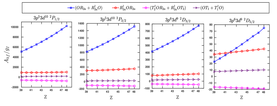
Figure 1: (color online) Plots showing the contributions from different dominant RCC terms such as ($OR_{2a}+R_{2a}^{\dagger}O$), ($OT_{1}+T_{1}^{\dagger}O$), $R_{2a}^{\dagger}OR_{2a}$ and ($R_{2a}^{\dagger}OT_{2}+T_{2}^{\dagger}OR_{2a}$) in the calculations of the ratios $A_{hf}/g_{I}$ (in MHz) for the calculated states against the atomic number $Z$ of the considered ions.

V Results and Discussion

As mentioned earlier, we calculate first the ground state configurations of the ions having Ni isoelectronic sequence and then, atomic state of the Co-like ions are determined by removing an electron from the occupied orbitals of the Ni-like ions. In this process, we obtain the first IPs of the respective Ni-like ions. However, the differential values between the IPs of different orbitals correspond to the EEs of the Co-like ions. The calculated IPs for the electrons in the $d_{5/2}$, $d_{3/2}$, $p_{3/2}$ and $p_{1/2}$ orbitals giving rise to the $3p^{6}3d^{9}\ {}^{2}D_{5/2}$, $3p^{6}3d^{9}\ {}^{2}D_{3/2}$, $3p^{5}3d^{10}\ {}^{2}P_{3/2}$ and $3p^{5}3d^{10}\ {}^{2}P_{1/2}$ atomic states of the investigated Co-like ions are given in the Table 1 from the DHF, RMBPT(2) and RCCSD methods. Contributions from the leading order relativistic corrections such as Breit interaction ($\Delta E_{B}$), VP effect ($\Delta E_{VP}$) and SE effect ($\Delta E_{SE}$) are also estimated and quoted in the above table explicitly. From these tabulated values for IPs, we find after the Coulomb interactions the Breit interactions also contribute significantly to the energy. There are large cancellations among the VP and SE effects of the QED interactions. These IP values also show that the DHF method overestimates the energies, while there is a gradual decrease in the values from the RMBPT(2) to RCCSD methods using the DC Hamiltonian. Further analysis demonstrates that contributions from the correlation and the relativistic effects are increasing from the ground state to the excited states. The trends of the correlation effects are found to be similar in all the considered Co-like ions using our RCC theory.

We present the final values of the IPs of all the four low-lying states for the investigated ions in Table 1 by adding contributions from the DC Hamiltonian and corrections from the Breit, VP, and SE interactions. We have also estimated uncertainties to the total values by analyzing contributions due to the truncation of basis functions and neglected higher-level excitations in the RCC theory. The basis function extrapolations are obtained using a lower-order many-body method while we have estimated uncertainties due to the higher level excitations by analyzing contributions from the dominant triple excitations by adopting the perturbative approach. Our final values are also compared with the IPs of the only available data for the $3p^{6}3d^{9}\ {}^{2}D_{5/2}$ states for all the ions from the National Institute of Science and Technology (NIST) database Kramida et al. (2020). These values were obtained using the non-relativistic Hartree-Fock orbitals, so we see large differences among these values. Nonetheless, IPs for the orbitals giving rise to the other states of Co-like ions are not available for comparison.

It can be obvious from the above discussions on IPs that EEs, which are obtained from the differences of IPs, are more relevant quantities here as they are directly related to the investigated Co-like ions. In Table 3, we compare our calculated EEs with a few available experimental results. Only a few direct measurements of excitation energies are reported, while the other experimental values are extrapolated by fitting the calculated wavelengths with some of the observed wavelengths. So far, the direct measurements were carried out only for the ions Zr¹³⁺, Mo¹⁵⁺, and Nb¹⁴⁺. Edlén Edlén (1984) had measured the forbidden lines of the Zr¹³⁺ and Mo¹⁵⁺ ions in a hot tokamak plasma experiment, while Prior Prior (1987) had directly obtained the EEs of Nb¹⁴⁺ by performing measurement using the electron cyclotron resonance ion source. The indirectly inferred values are quoted in the above table as ‘Fitted’, which had used calculations using the MCDHF method to extrapolate EEs of all the considered ions Ekberg et al. (1987). Comparison between our calculated values with the measurements shows good agreement between them suggesting our calculations for the transition matrix elements using the RCC theory can be accurate enough to estimate the transition properties of the excited states. This also suggests that the inclusion of triple excitations in our RCC calculations can improve our results further.

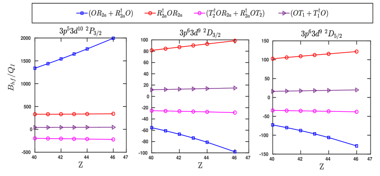
Figure 2: (color online) Plots showing the contributions from different dominant RCC terms such as ($OR_{2a}+R_{2a}^{\dagger}O$), ($OT_{1}+T_{1}^{\dagger}O$), $R_{2a}^{\dagger}OR_{2a}$ and ($R_{2a}^{\dagger}OT_{2}+T_{2}^{\dagger}OR_{2a}$) in the evaluation of the ratios $B_{hf}/Q_{I}$ (in MHz) against the atomic number $Z$ of the Zr¹³⁺, Nb¹⁴⁺, Mo¹⁵⁺, Tc¹⁶⁺, Ru¹⁷⁺, and Pd¹⁹⁺ ions. Since, $I=1/2$, for the ions ${}^{89}_{39}$Y¹²⁺, ${}^{103}_{45}$Rh¹⁸⁺, ${}^{109}_{47}$Ag²⁰⁺, and ${}^{111}_{48}$Cd²¹⁺, so the $Q_{I}$ value for them do not exist. This is why we have excluded the calculation of the $B_{hf}/Q_{I}$ ratios for these ions.

After analyzing the accuracies of the calculated EEs using our RCCSD method, we now proceed to calculate other transition properties such as the line strengths, transition probabilities, oscillator strengths, and lifetimes of the excited states of the considered Co-like ions. We also present the hyperfine structure constants of all the calculated states. The transition properties such as the line strengths, oscillator strengths, transition probabilities, and lifetimes of the excited states are presented in Table 4. First, the line strengths are determined using the calculated reduced matrix elements of the E1, E2, and M1 operators. Substituting these values, we obtained the other transition properties. In order to reduce the uncertainties, we have used the wavelengths from the NIST database in estimating these values. Earlier, lifetimes of the fine structure level of the ground state of the aforementioned ions were estimated by applying the MCDHF method, and we found reasonable agreement among our values with the previously estimated values. In the earlier estimations, contributions from the E2 channel were neglected and our analysis shows that they are indeed small. The lifetimes of the $3p^{5}3d^{10}\ {}^{2}P_{3/2}$ and $3p^{5}3d^{10}\ {}^{2}P_{1/2}$ states are not available to date, so we are unable to make a comparative analysis of these values. In the determination of lifetimes of the $3p^{5}3d^{10}\ {}^{2}P_{1/2}$ states, we have also accounted for the transition probabilities due to the forbidden channels but their contributions are found to be negligibly small compared to the E1 probability contributions. The E1 transition probabilities of the $3p^{5}3d^{10}\ {}^{2}P_{3/2}\rightarrow 3p^{6}3d^{9}\ {}^{2}D_{5/2}$ transitions are found to be dominant over the $3p^{5}3d^{10}\ {}^{2}P_{1/2}\rightarrow 3p^{6}3d^{9}\ {}^{2}D_{5/2}$ transitions. Though there are two E1 transitions are allowed from the $3p^{5}3d^{10}\ {}^{2}P_{3/2}$ state than the $3p^{5}3d^{10}\ {}^{2}P_{1/2}$, the lifetimes of the $3p^{5}3d^{10}\ {}^{2}P_{1/2}$ states in the Co-like ions are found to be smaller than the $3p^{5}3d^{10}\ {}^{2}P_{3/2}$ states. We also find that the E1 transition probabilities are larger when the angular momentum difference is $|\Delta J=1|$ than $|\Delta J=0|$. Further, due to the monotonic increase in the energy gap between the $3p^{5}3d^{10}\ {}^{2}P_{3/2}$ and the $3p^{6}3d^{9}\ {}^{2}D_{5/2}$ ground state with the size of the ion, the transition probabilities gradually increase from Y¹²⁺ to Tc¹⁶⁺. This results in smaller values of the lifetimes of the atomic states with increasing ionic charge of the Co-like systems.

Table 7: The estimated values of $A_{hf}$ and $B_{hf}$ for the calculated states of the Co-like ions using the RCCSD method. The nuclear parameters for the stable isotopes used to estimate these values are taken from Ref. Stone (2005) and they are listed here. As can be seen the reported $Q_{I}$ values of the ${}^{91}_{40}$Zr¹³⁺ and ${}^{97}_{42}$Mo¹⁵⁺ isotopes differ significantly from various works, so we present the $B_{hf}$ values for these ions by considering all the reported values of $Q_{I}$. We anticipate that the $Q_{I}$ values of these isotopes can be inferred more reliably by combining our calculations with possible measurements of the $B_{hf}$ values in these ions.

Ion	$I$	$\mu_{I}$	$g_{I}$		$A_{hf}$ (in MHz)				$Q_{I}$ (in $b$)		$B_{hf}$ (in MHz)
				${}^{2}D_{5/2}$	${}^{2}D_{3/2}$	$\ {}^{2}P_{3/2}$	${}^{2}P_{1/2}$			${}^{2}D_{5/2}$	${}^{2}D_{3/2}$	${}^{2}P_{3/2}$
${}^{89}_{39}$Y12+	$\frac{1}{2}$	$-0.1374154(3)$	$-0.2748308$	$-756$	$-1897$	$-4494$	$-25816$
${}^{91}_{40}$Zr13+	$\frac{5}{2}$	$-1.30362(2)$	$-0.521448$	$-1617$	$-4049$	$-9426$	$-54578$		$-0.176(3)$	$-1098$	$-801$	$-5893$
									$-0.257(13)$	$-1604$	$-1170$	$-8606$
									$-0.206(10)$	$-1285$	$-938$	$-6898$
${}^{93}_{41}$Nb14+	$\frac{9}{2}$	$+6.1705(3)$	$1.37122$	$4767$	$11920$	$27331$	$159433$		$-0.37(2)$	$-2590$	$-1893$	$-13692$
${}^{97}_{42}$Mo15+	$\frac{5}{2}$	$-0.9335(1)$	$-0.37340$	$-1449$	$-3618$	$-8185$	$-48139$		$0.255(13)$	$1992$	$1460$	$10399$
									$0.17(4)$	$1328$	$973$	$6932$
									$0.27(10)$	$2109$	$1546$	$11011$
${}^{99}_{43}$Tc16+	$\frac{9}{2}$	$+5.6847(4)$	$1.263266$	$5448$	$13595$	$30374$	$180150$		$-0.129(6)$	$-1120$	$-823$	$-5782$
${}^{101}_{44}$Ru17+	$\frac{5}{2}$	$-0.719(6)$	$-0.28760$	$-1373$	$-3425$	$-7566$	$-45290$		$0.46(2)$	$4424$	$3257$	$22605$
${}^{103}_{45}$Rh18+	$\frac{1}{2}$	$-0.8840(2)$	$-1.7680$	$-9312$	$-23219$	$-50779$	$-306730$
${}^{105}_{46}$Pd19+	$\frac{5}{2}$	$-0.642(3)$	$-0.25680$	$-1487$	$-3708$	$-8034$	$-48990$		$0.660(11)$	$7703$	$5701$	$38715$
									$0.65(3)$	$7587$	$5615$	$38129$
${}^{109}_{47}$Ag20+	$\frac{1}{2}$	$-0.1306906(2)$	$-0.2613812$	$-1659$	$-4138$	$-8888$	$-54799$
${}^{111}_{48}$Cd21+	$\frac{1}{2}$	$-0.5948861(8)$	$-1.1897722$	$-8258$	$-20588$	$-43893$	$-272786$

Now we turn on to present the results for the hyperfine structure constants of the considered Co-like ions. The accuracies of the transition matrix elements discussed earlier depend on the accurate determinations of the wave functions in the asymptotic region while accuracies in the evaluation of the hyperfine structure constants depend on the accurate calculations of the wave functions in the nuclear region. The determination of the hyperfine structure constants not only depends on the accurate calculations of the atomic matrix elements but also requires knowledge of accurate values of the nuclear moments. Since we are interested to estimate the $A_{hf}$ and $B_{hf}$ values, we need prior knowledge of $g_{I}=\frac{\mu_{I}}{I}$ and $Q_{I}$ of the isotopes of the interest. This implies the $A_{hf}$ and $B_{hf}$ values are isotope dependent. However, the calculations of the $A_{hf}/g_{I}$ and $B_{hf}/Q_{I}$ values hardly change with the nuclear structure of the isotopes of an element. Thus, we discuss first these results and then present the estimated $A_{hf}$ and $B_{hf}$ value only for the stable isotopes of the elements of the investigated Co-like ions by combining with their respective $g_{I}$ and $Q_{I}$ values. Our calculated values of $A_{hf}/g_{I}$ and $B_{hf}/Q_{I}$ are reported in Table 6 for all the considered atomic states of the Co-like Y¹²⁺ - Cd²¹⁺ ions. We have not given the $B_{hf}/Q_{I}$ values of the Y¹²⁺, Rh¹⁸⁺, Ag²⁰⁺ and Cd²¹⁺ ions as their $B_{hf}$ values do not exist owing to the fact that they all have $I=1/2$. It can be observed from this table that the DHF values for $A_{hf}/g_{I}$ are smaller than the RCCSD results for all the states, which are opposite to the trends seen in the calculations of IPs. The values and the electron correlation effects increase from the ground to the higher excited states. The reason for the large magnitude is due to the fact that the $3d$ orbitals have less overlap with the nucleus than the $3p$ orbitals, which are the valence orbitals of the first and the last two states respectively. The possible reason for which the correlation effects are seen to be enhanced in the calculations of the hyperfine structure constants for the ground state to the higher level excited states are probably due to the large correlations among the $s$ and $p$ orbitals than the $s$ and $d$ orbitals. Again, the values of the above quantities are found to be increasing with the size of the ion. The reason for this could be due to highly contracted orbitals in the more highly charged ions that can overlap with the nucleus strongly.

We also intend to fathom the roles of different electron correlation effects in the atomic states of Co-like ions. Evaluation of transition matrix elements depends on the wave functions of two different atomic states, while the determination of hyperfine structure constants of a state depends only on the wave function of the respective state. Thus, we analyze the contributions to the $A_{hf}/g_{I}$ and $B_{hf}/Q_{I}$ values arising through various RCCSD terms. Instead of quoting them in tables, we show their contributions to the $A_{hf}/g_{I}$ and $B_{hf}/Q_{I}$ values in the graphical representations in Figs. 1 and 2, respectively, against the atomic number. Among all property evaluating RCC terms, we find that the $OR_{2a}$, $OT_{1}$, $R_{2a}^{\dagger}OR_{2a}$ and $R_{2a}^{\dagger}OT_{2}$ terms along with their hermitian conjugate (h.c.) contribute predominantly to the above quantities. The term representing $OR_{2a}$ accounts for the core-polarization effects to all-orders, while the $OT_{1}$ term represents for the extra core-valence correlation effects that were accounted in the calculations of the ground states of the corresponding Ni-like ions from which atomic states of the Co-like ions were derived. The other two non-linear terms, $R_{2a}^{\dagger}OR_{2a}$ and $R_{2a}^{\dagger}OT_{2}$, are responsible for including higher-order core-polarization effects in our calculations. It can be seen from Fig. 1 that the most dominating term is the core-polarization term $OR_{2a}$ for all the atomic states that further show an increasing trend with atomic number. As expected, the effect of the core-polarization for the outermost $d-$orbitals are comparatively quite smaller than the inner valence $p-$orbitals, so the contribution to the $A_{hf}/g_{I}$ values are quite large for the $3p^{5}3d^{10}\ {}^{2}P_{1/2,3/2}$ excited states. The next dominating contribution comes from the non-linear term $R_{2a}^{\dagger}OR_{2a}$ although the magnitude is smaller compared to the core-polarization effect except for the ground states with $Z=39$, $40$ and $41$. The other non-linear term, $R_{2a}^{\dagger}OT_{2}$, also contributes significantly however, the values show an opposite behavior (i.e. negative value) compared to the other three terms. Finally, the core-valence correlation effects through $OT_{1}$ seem to give non-negligible contribution to $A_{hf}/g_{I}$.

We now would like to discuss the behavior of the above dominating terms for the calculations of $B_{hf}/Q_{I}$ and the contributions from the above RCC terms to this quantity are plotted in Fig. 2. The behavior for the core-polarization effect in determining the $B_{hf}/Q_{I}$ values are found to be quite similar to that of $A_{hf}/g_{I}$ for the excited state $3p^{5}3d^{10}\ {}^{2}P_{3/2}$ although they differ in the magnitudes percentage-wise. In contrast, for the ground state doublets, the core-polarization trend shows an opposite behavior as compared to the $A_{hf}/g_{I}$ values for the excited states. In fact, it shows an increasing trend in the negative direction with respect to the atomic number. The next leading order contributions to $B_{hf}/Q_{I}$ are given by the $R_{2a}^{\dagger}OR_{2a}$ term which further show that for the state $3p^{5}3d^{10}\ {}^{2}P_{3/2}$ their magnitudes are nearly equal for all the investigated ions. On contrary, for the ground state doublets, the corresponding values are slowly increasing as a function of $Z$. There are also finite contributions coming from the non-linear term $R_{2a}^{\dagger}OT_{2}$ that show an almost constant trend in the respective states with the increase in atomic number. The core-valence term $OT_{1}$ also gives non-negligible contributions to the $B_{hf}/Q_{I}$ values for all the states.

As mentioned earlier, the quantities of experimental interest are the $A_{hf}$ and $B_{hf}$ values. To obtain these values from our calculations of $A_{hf}/g_{I}$ and $B_{hf}/Q_{I}$, we used the nuclear moments that are listed in the nuclear data table Stone (2005) for the most stable isotopes. We have given the final $A_{hf}$ and $B_{hf}$ values for all the four calculated states by combining our RCCSD values of atomic calculations and nuclear moments in Table 7. Due to the fact that $I=1/2$, the $B_{hf}$ values do not exist for Y¹²⁺, Rh¹⁸⁺, Ag²⁰⁺ and Cd²¹⁺. The nuclear moments for the stable isotopes for which we have determined the hyperfine structure constants are also listed in the above table. It can be seen that the $\mu_{I}$ values are known very precisely for these isotopes, but many different $Q_{I}$ values are reported for a few isotopes; especially for ${}^{91}_{40}$Zr¹³⁺ and ${}^{97}_{42}$Mo¹⁵⁺. So we suggest that if the $B_{hf}$ of either of the $3p^{6}3d^{9}\ {}^{2}D_{5/2}$, $3p^{6}3d^{9}\ {}^{2}D_{3/2}$ or $3p^{5}3d^{10}\ {}^{2}P_{3/2}$ state is measured precisely for the above ion, then by combining that measured value with our $B_{hf}/Q_{I}$ calculation it is possible to infer the $Q_{I}$ value of the respective ion more reliably.

VI Conclusion

We have employed the Fock-space relativistic coupled-cluster method to calculate the atomic wave functions of the first four low-lying $3p^{6}3d^{9}\ {}^{2}D_{5/2}$, $3p^{6}3d^{9}\ {}^{2}D_{3/2}$, $3p^{5}3d^{10}\ {}^{2}P_{3/2}$ and $3p^{5}3d^{10}\ {}^{2}P_{1/2}$ states of the Co-like ions such as Y¹²⁺, Zr¹³⁺, Nb¹⁴⁺, Mo¹⁵⁺, Tc¹⁶⁺, Ru¹⁷⁺, Rh¹⁸⁺, Pd¹⁹⁺, Ag²⁰⁺ and Cd²¹⁺, which are one electron less than a closed-shell electronic configuration. The Dirac-Breit interactions along with lower-order QED effects through an effective potential are considered to perform these calculations. Only the dominant singles and doubles excitation configurations were taken into account in our method, and the uncertainties were estimated by analyzing leading order contributions from the valence triple excitations and truncated basis functions. The ionization potentials of the Ni-like ions of the above elements were first determined in order to obtain the considered atomic states of Co-like ions, and taking their differences the excitation energies of the respective Co-like ions were estimated. Further, the calculated wave functions were used to determine the E1, E2, and M1 transition matrix elements among the aforementioned states of the Co-like ions. Further, using these matrix elements we determine other transition properties such as the line strengths, oscillator strengths, and transition probabilities. The lifetimes of the excited states were estimated from the total transition probabilities from a given excited state and they are compared with the available theoretical values. In addition, we have also determined the magnetic-dipole and electric-quadrupole hyperfine structure constants of the above states of the stable isotopes of Co-like ions. Since the nuclear quadrupole moment of the ${}^{91}_{40}$Zr and ${}^{97}_{42}$Mo isotopes are not known precisely, we suggest to infer their values by combining our calculations of $B_{hf}/Q_{I}$ of one of its states with the measurement of $B_{hf}$ of the corresponding state in the future.

References

- Pütterich et al. (2005) T. Pütterich, R. Neu, C. Biedermann, R. Radtke, and A. U. Team, Journal of Physics B 38, 3071 (2005).
- Yanagibayashi et al. (2010) J. Yanagibayashi, T. Nakano, A. Iwamae, H. Kubo, M. Hasuo, and K. Itami, Journal of Physics B 43, 144013 (2010).
- Sudkewer (1981) S. Sudkewer, Physica Scripta 23, 72 (1981).
- Suckewer and Hinnov (1979) S. Suckewer and E. Hinnov, Phys. Rev. A 20, 578 (1979).
- Biémont and Zeippen (1996) E. Biémont and C. J. Zeippen, Physica Scripta T65, 192 (1996).
- Utter et al. (2000) S. B. Utter, P. Beiersdorfer, and G. V. Brown, Phys. Rev. A 61, 030503 (2000).
- Porto et al. (2000) J. V. Porto, I. Kink, and J. D. Gillaspy, Phys. Rev. A 61, 054501 (2000).
- Ralchenko et al. (2006) Y. Ralchenko, J. N. Tan, J. D. Gillaspy, J. M. Pomeroy, and E. Silver, Phys. Rev. A 74, 042514 (2006).
- Gillaspy et al. (2009) J. D. Gillaspy, I. N. Draganić, Y. Ralchenko, J. Reader, J. N. Tan, J. M. Pomeroy, and S. M. Brewer, Phys. Rev. A 80, 010501 (2009).
- Harte et al (2010) C. S. Harte et al, J. Phys. B: At. Mol. and Opt. Phys. 43, 205004 (2010).
- Nandy and Sahoo (2016a) D. K. Nandy and B. K. Sahoo, Phys. Rev. A 94, 032504 (2016a).
- Yu and Sahoo (2019a) Y.-m. Yu and B. K. Sahoo, Phys. Rev. A 99, 022513 (2019a).
- Yu and Sahoo (2018) Y.-m. Yu and B. K. Sahoo, Phys. Rev. A 97, 041403 (2018).
- Yu and Sahoo (2016) Y.-m. Yu and B. K. Sahoo, Phys. Rev. A 94, 062502 (2016).
- Safronova et al. (2014) M. S. Safronova, V. A. Dzuba, V. V. Flambaum, U. I. Safronova, S. G. Porsev, and M. G. Kozlov, Phys. Rev. A 90, 042513 (2014).
- Berengut et al. (2012) J. C. Berengut, V. A. Dzuba, V. V. Flambaum, and A. Ong, Phys. Rev. A 86, 022517 (2012).
- Dzuba and Flambaum (2017) V. A. Dzuba and V. V. Flambaum, in TCP 2014, edited by M. Wada, P. Schury, and Y. Ichikawa (Springer International Publishing, Cham, 2017) pp. 79–86.
- Berengut et al. (2010) J. C. Berengut, V. A. Dzuba, and V. V. Flambaum, Phys. Rev. Lett. 105, 120801 (2010).
- Feldman et al. (1991) U. Feldman, P. Indelicato, and J. Sugar, J. Opt. Soc. Am. B 8, 3 (1991).
- Nandy and Sahoo (2013) D. K. Nandy and B. K. Sahoo, Phys. Rev. A 88, 052512 (2013).
- Nandy, D. K. and Sahoo, B. K. (2014) Nandy, D. K. and Sahoo, B. K., A&A 563, A25 (2014).
- Nandy and Sahoo (2016b) D. K. Nandy and B. K. Sahoo, Phys. Rev. A 94, 032504 (2016b).
- Nandy (2016) D. K. Nandy, Phys. Rev. A 94, 052507 (2016).
- Cheung et al. (2020) C. Cheung, M. S. Safronova, S. G. Porsev, M. G. Kozlov, I. I. Tupitsyn, and A. I. Bondarev, Phys. Rev. Lett. 124, 163001 (2020).
- Ralchenko et al. (2011) Y. Ralchenko, I. N. Draganić, D. Osin, J. D. Gillaspy, and J. Reader, Phys. Rev. A 83, 032517 (2011).
- Ding et al. (2012) X.-B. Ding, F. Koike, I. Murakami, D. Kato, H. A. Sakaue, C.-Z. Dong, and N. Nakamura, J. Phys. B: At. Mol. and Opt. Phys. 45, 035003 (2012).
- Suckewer et al. (1982) S. Suckewer, E. Hinnov, S. Cohen, M. Finkenthal, and K. Sato, Phys. Rev. A 26, 1161 (1982).
- Prior (1987) M. H. Prior, J. Opt. Soc. Am. B 4, 144 (1987).
- Edlén (1984) B. Edlén, Physica Scripta T8, 5 (1984).
- Ekberg et al. (1987) J. O. Ekberg, U. Feldman, J. F. Seely, C. M. Brown, J. Reader, and N. Acquista, J. Opt. Soc. Am. B 4, 1913 (1987).
- Alexander et al. (1971) E. Alexander, M. Even-Zohar, B. S. Fraenkel, and S. Goldsmith, J. Opt. Soc. Am. 61, 508 (1971).
- Burkhalter et al. (1980) P. Burkhalter, J. Reader, and R. D. Cowan, J. Opt. Soc. Am. 70, 912 (1980).
- Guo et al. (2016) X. L. Guo, R. Si, S. Li, M. Huang, R. Hutton, Y. S. Wang, C. Y. Chen, Y. M. Zou, K. Wang, J. Yan, C. Y. Li, and T. Brage, Phys. Rev. A 93, 012513 (2016).
- Grant et al. (1980) I. Grant, B. McKenzie, P. Norrington, D. Mayers, and N. Pyper, Computer Physics Communications 21, 207 (1980).
- Kramida et al. (2020) A. Kramida, Yu. Ralchenko, J. Reader, and and NIST ASD Team, NIST Atomic Spectra Database (ver. 5.8), [Online]. Available: https://physics.nist.gov/asd [2021, August 12]. National Institute of Standards and Technology, Gaithersburg, MD. (2020).
- Grant (2007) I. P. Grant, Relativistic Quantum Theory of Atoms and Molecules (Springer, New York, NY, 2007).
- Ginges and Berengut (2016) J. S. M. Ginges and J. C. Berengut, Phys. Rev. A 93, 052509 (2016).
- Yu and Sahoo (2019b) Y.-m. Yu and B. K. Sahoo, Phys. Rev. A 99, 022513 (2019b).
- Lindgren and Morrison (1986) I. Lindgren and J. Morrison, Atomic Many-Body Theory (Springer-Verlag, Berlin, Germany, 1986).
- Reiher and Wolf (2014) M. Reiher and A. Wolf, Relativistic Quantum Chemistry: The Fundamental Theory of Molecular Science (WILEY-VCH Verlag, Germany, 2014).
- Johnson (2007) W. R. Johnson, Atomic Structure Theory (Springer-Verlag, Berlin, Germany, 2007).
- Shavitt and Bartlett (2009) I. Shavitt and R. J. Bartlett, Many-Body Methods in Chemistry and Physics: MBPT and Coupled-Cluster Theory (Cambridge University Press, Cambridge, 2009).
- Sahoo et al. (2004) B. K. Sahoo, S. Majumder, R. K. Chaudhuri, B. P. Das, and D. Mukherjee, J. Phys. B: At. Mol. and Opt. Phys. 37, 3409 (2004).
- Sobelman (1979) I. I. Sobelman, Atomic Spectra and Radiative Transitions (Springer-Verlag, Berlin, Germany, 1979).
- Schwartz (1955) C. Schwartz, Phys. Rev. 97, 380 (1955).
- Stone (2005) N. Stone, Atomic Data and Nuclear Data Tables 90, 75 (2005).