QoS-Oriented Sensing-Communication-Control Co-Design for UAV-Enabled Positioning

Abstract

Unmanned aerial vehicle (UAV)-enabled positioning that uses UAVs as aerial anchor nodes is a promising solution for providing positioning services in harsh environments. In previous research, the state sensing and control of UAVs were either ignored or simply set to be performed continuously, resulting in system instability or waste of wireless resources. Therefore, in this article, we propose a quality-of-service (QoS)-oriented UAV-enabled positioning system based on the concept of sensing-communication-control (SCC) co-design. We first establish the mathematical models of UAV state sensing and control. Then, the influence of sensing scheduling and transmission failure on UAV stability, as well as the performance of positioning services in the presence of UAV control error, are analyzed. Based on these models and analysis results, we further study the problem of minimizing the amount of data transmitted by optimizing the sensing scheduling and blocklength allocation under the condition of satisfying each user’s demand. Finally, an efficient scheme is developed to solve this mixed-integer nonlinear problem. Numerical results show that the proposed system could work efficiently and meet users’ requirements. In addition, compared with two benchmark schemes, our scheme reduces the failure rate or resource consumption of positioning services by more than 76.2$\%$ or 82.7$\%$.

I Introduction

I-A Motivation

As the efficiency and intelligence of industrial manufacturing and people’s daily lives has been improved continuously by location-based services (LBS) like logistic tracking and mobile marketing, positioning technology is playing an increasingly important role in this mobile information era [1]. Therefore, ubiquitous positioning has been recognized as an essential service and an enabling technology by both the current fifth generation (5G) wireless networks and the future six generation (6G) communications [2, 3]. Unfortunately, conventional wireless positioning technologies represented by global navigation satellite system (GNSS) and cellular-based positioning may suffer severe performance degradation in some harsh environments like dense urban and fail to meet application requirements. For the widely used GNSS systems, their signals are easily blocked or reflected by buildings or rugged terrain, resulting in multipath or none-line-of-sight (NLoS) propagation that cause large position errors [4]. Moreover, due to frequent signal blockages, the geometry of satellites available to users is often unsuitable for positioning [5]. Similarly, the above problems, including NLoS propagation, insufficient number and unsatisfactory geometry of base stations (BS) can also be found in cellular-based positioning, which severely affect the positioning accuracy [6, 7, 8]. Thus, we need a better platform to provide wireless positioning services in harsh environments.

Due to their high operational flexibility and fully controllable mobility, unmanned aerial vehicles (UAV) have recently received considerable attention from the research community and may help create a whole new paradigm for wireless networks [9]. In the past few years, researchers have studied the potential of UAVs as aerial BSs, relays and data collectors to provide services for ground users or assist terrestrial networks [10, 11, 12]. It is noteworthy that in addition to their use for communication, UAV could also be a promising platform for positioning [13]. Unlike satellites operating in fixed orbits or BSs that cannot be moved, UAVs with high maneuverability can fly close to users, making the number of available anchor nodes sufficient for positioning [14]. Moreover, UAVs are more likely to establish line-of-sight (LoS) links with ground users than terrestrial BSs due to their relatively high flying altitudes [9]. In addition, by considering UAV-user geometry in the deployment of UAVs, the problem of poor geometry common in conventional positioning technologies can also be largely avoided [15]. Therefore, UAV-enabled positioning that uses UAVs as aerial anchor nodes could be a good choice for positioning in challenging environments.

As typical automatic systems, the operation of UAVs or UAV swarms requires appropriate design and coordination of sensing, communication and control functionalities [16]. In existing systems, these three functionalities were commonly designed and implemented separately, which was previously thought to be conducive to ensuring compatibility among different functionalities [17]. Recently, many studies pointed out that considering the co-existence and cooperation of multiple functionalities at the beginning of system design can help improve system performance or resource efficiency [17, 18]. Thus, sensing-communication co-design (also called integrated sensing and communication) that enables the network and users to sense their dynamic states or the surrounding environment has been widely viewed as a key driver in future 6G networks [19]. The capability of state sensing helps to reduce the energy or resource consumption in wireless networks, and location-aided resource scheduling is a good application example [20]. Similarly, control and communication functionalities can also be considered jointly to provide extra design freedom for future automatic systems. Recent research indicated that control-communication co-design could address problems existing in a single functionality, or even create new applications by taking advantage of the imperfections of each functionality [17]. Moreover, if the communication functionality is designed based on system’s actual needs for control, the current stringent requirements on communication latency and reliability can be greatly relaxed, thereby reducing unnecessary resource consumption [21]. Therefore, it is very promising to develop sensing-communication-control (SCC) co-design solutions for UAV-related applications [20, 22].

I-B Related Work

As society’s demand for ubiquitous positioning services increases continuously, UAV-enabled positioning has recently become a hot topic for research due to its high flexibility and adaptability in harsh environments. Sallouha et al. [23] proposed a UAV-enabled positioning system that utilizes the received-signal-strength (RSS) technique to locate ground users in urban areas and derived the corresponding theoretical performance limits. In [24], the UAV trajectory in the same system was optimized to find a good balance between the accuracy of RSS-based two-dimensional (2-D) positioning and UAVs’ propulsion energy consumption. Wang et al. [14] introduced the time-difference-of-arrival (TDoA) approach into UAV-enabled positioning and realized high-accuracy 3-D localization by exploiting the vertical diversity of UAV platforms. Moreover, in [15], the reliability of UAV-enabled positioning services in mountainous areas was modeled and enhanced. In these studies, UAVs were treated as anchor nodes with perfect knowledge of their own positions. In practice, UAVs’ positions are commonly obtained through state sensing, and the inevitable sensing errors will cause uncertainty in anchor position information [25, 26]. Thus, the authors in [25] studied the problem of UAV self-localization and evaluated the impact of UAV position uncertainty on positioning performance. Furthermore, Liu et al. [26] proposed a deployment optimization method considering UAV position uncertainty to improve the accuracy of UAV-enabled positioning. These two studies assume that UAVs can hover stably at fixed positions, which is not true in practical applications due to unintentional movements caused by environmental factors like wind. Hence, the authors in [27] quantitatively analyzed the influence of the instability and mobility of UAV platforms on UAV relative localization. However, in this study, the anchor position uncertainty in different directions caused by UAV instability was simply modeled as independent Gaussian random variables with the same variance, which may be too optimistic for practice. Therefore, in order to ensure the practicability of UAV-enabled positioning, both the state sensing error and control error should be taken into consideration in system design, and they should be modeled objectively according to the system dynamics model and control policy.

In terms of the co-design of different functionalities, several successful attempts have been made in recent years. In [28], the authors achieved the co-existence between radar and communication systems through cooperative spectrum sharing, and studied the problem of cross interference management. The two systems studied in this research still work separately on different platforms for different users. No other interactions between the sensing and communication functionalities were considered in this study except for the cross interference. Liu et al. [29] integrated radar sensing and millimeter wave (mmWave) communication functionalities on a multiple-input multiple-output (MIMO) system, and designed the corresponding frame structure. Nevertheless, in this study, the users or targets of the two functionalities are different, which means that a single user cannot benefit from both functionalities. In [30], the vehicle motion predicted through radar sensing was used to assist the reception of downlink communication signals. Unfortunately, controls issues are not considered in this study, making the vehicle dynamics model used less practical. Mei et al. [31] and González et al. [32] introduced the communication-control co-design into vehicle-to-vehicle (V2V) networks, and developed resource scheduling algorithms to ensure the string stability of vehicle platoons. In these two studies, the sensing of each vehicle’s kinematic status was assumed to be performed perfectly without failures or errors, which is not true in practical applications. In [33] and [34], control-aware communication was used to improve the resource efficiency of wireless control systems. These two studies focused on the stability and resource consumption of a control system, rather than the system’s ability to perform the required tasks. In fact, a system may not need to be very stable to provide services that satisfy users’ demands, and stringent requirements on stability may lead to a waste of resources. From the above analysis, it can be concluded that if we want to improve the performance or efficiency of an automatic system through the joint design of multiple functionalities, the following requirements need to be met in system design.

• Essential functionalities including sate sensing, communication and control should be comprehensively considered.

• The imperfections of each functionality should be modeled objectively.

• The main consideration should be the performance of the services provided for users.

I-C Main Contributions

In this article, a quality-of-service (QoS)-oriented UAV-enabled positioning system is proposed based on the idea of SCC co-design to improve the resource efficiency of positioning services while ensuring that users’ requirements on positioning accuracy are met. To evaluate objectively the performance of our system in practical applications, we consider the impact of UAV position uncertainty caused by the state sensing error and control error on positioning. Specifically, the mathematical models of UAV state sensing and control in two operation modes, “open-loop” and “closed-loop”, are first established. Based on these models, we further derive the covariance matrices of UAV control errors in different operation modes, as well as the mean-square error (MSE) of positioning services in the presence of UAV position uncertainty. It is found that the quality of positioning services is mainly determined by UAVs’ operation modes, while the latter depends on the scheduling of UAV state sensing and successful transmissions of sensing data with finite blocklength, resulting in the coupling among sensing, communication and control functionalities. Then, we try to reduce the resource consumption for positioning services by reducing the frequency of state sensing and the blocklength for data transmission, while ensuring that users’ QoS demands are satisfied. This work is formulated as a mixed-integer nonlinear optimization problem, and an efficient scheme is developed to solve it.

In a nutshell, the major contributions of this article are listed as follows:

• Different from previous studies that treated UAVs as perfect anchor nodes, we consider UAV position uncertainty caused by the state sensing error and control error in system design and analysis. In particular, the imperfections of each functionality are modeled objectively, making our system more practical than existing ones.

• We derive the covariance matrices of UAV position uncertainty and the MSE of positioning services in different operation modes. These derivations can be used as a general framework for the design and analysis of UAV-enabled positioning systems, and provide guidance for future research on SCC co-design like resource allocation.

• When solving the problem of sensing scheduling and blocklength allocation, we develop a scheme that converts the constraint on the positioning MSE of each user into the constraint on each UAV’s control error. This scheme decouples the control of each UAV, and is therefore suitable for large-scale UAV-enabled positioning systems.

Numerical results demonstrate that our proposed system and scheme achieve the desired results in terms of QoS and resource efficiency. Moreover, compared with two benchmark schemes, the proposed scheme achieves significantly lower failure rate or better resource efficiency. To the best of our knowledge, this work is the first to introduce the concept of sensing-communication-control co-design into UAV-enabled positioning.

Notations: In this article, scalars are denoted by italic letters ($x$). Lowercase and uppercase boldface letters (${\bf{x}}$ and ${\bf{X}}$) are used to denote column vectors and matrices, respectively. ${\mathbb{R}^{N\times 1}}$ represents the space of $N$-dimensional real-valued vectors. The superscript $T$ indicates the transpose operation (${{\bf{X}}^{T}}$) and superscript $-1$ indicates matrix inverse (${{\bf{X}}^{-1}}$). ${\left\|\cdot\right\|_{2}}$ and ${\mathop{\rm tr}\nolimits}\left(\cdot\right)$ denote the Euclidean norm and matrix trace, respectively. $E\left\{\cdot\right\}$ represents the statistical expectation operator and $P\left(\cdot\right)$ indicates the probability. ${\mathop{\rm diag}\nolimits}\left(\cdot\right)$ and ${\mathop{\rm blkdiag}\nolimits}\left(\cdot\right)$ denote the diagonal and block diagonal matrices, respectively. ${{\bf{I}}_{N}}$ is the $N\times N$ identity matrix and ${{\bf{0}}_{N\times M}}$ represents the $N\times M$ all-zero matrix. ${\cal N}\left({{{\bf{0}}_{N\times 1}},{\bf{Q}}}\right)$ denotes the $N$-dimensional Gaussian distribution with zero mean and covariance matrix ${\bf{Q}}$. $\dot{v}$ indicates the first-order derivative of the time-dependent function $v$ with respect to time.

II System Design

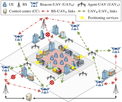
Figure 1: Proposed UAV-enabled positioning system.

In this article, as shown in Fig. 1, we consider a scenario where multiple ground users requiring positioning services are located in a challenging environment. In such an environment, conventional technologies such as GNSS and terrestrial cellular-based positioning fail to meet users’ requirements due to their drawbacks discussed in the previous section. Therefore, multiple low-altitude UAV platforms are employed as aerial anchor nodes to undertake the task of locating ground users. These UAVs can be classified into two groups according to their functions in the proposed system, namely the “agent UAV (UAV_A)” and “beacon UAV (UAV_B)”. Among them, UAV_A are responsible for providing positioning services to users. Since UAV_A are deployed close to ground users, the air-to-ground (A2G) links between UAV_A and user equipment (UE) are dominated by LoS components. However, due to their long distance from terrestrial BSs, UAV_A are unable to determine their own locations through cellular-based positioning. Thus, UAV_B whose locations have been accurately estimated and remain unchanged are used to provide UAV_A with relative range measurements required for state sensing.

The proposed system shown in Fig. 1 consists of ${N_{A}}$ UAV_A, ${N_{B}}$ UAV_B and $M$ UE. UAV_A and UAV_B are denoted by sets ${{\cal N}_{A}}=\left\{{1,\cdots,{N_{A}}}\right\}$ and ${{\cal N}_{B}}=\left\{{1,\cdots,{N_{B}}}\right\}$, respectively. The $j$-th UAV_A ($j\in{{\cal N}_{A}}$) is deployed at a carefully selected “hovering point (HP)”, which can be denoted by the horizontal coordinates ${\bf{q}}_{j}^{\circ}\in{\mathbb{R}^{2\times 1}}$ and height ${h_{v}}$. The 3-D coordinates of $j$-th UAV_A’s HP are denoted by ${\bf{q}}_{j}^{\circ,3D}\!=\!{\left[{{{\left({{\bf{q}}_{j}^{\circ}}\right)}^{T}},{h_{v}}}\right]^{T}}\!\in{\mathbb{R}^{3\times 1}}$. As mentioned in the previous section, in practice, UAV_A are unable to hover stably at fixed positions, and can only maintain themselves in close vicinity of the selected HPs through sensing and control functionalities. Moreover, it is assumed that UAV_A can maintain the preset altitude (${h_{v}}$) utilizing their onboard sensors like barometric altimeter. Then, we represent the true location of the $j$-th UAV_A in time slot $t$ as ${{\bf{q}}_{j,t}}\in{\mathbb{R}^{2\times 1}}$ (${\bf{q}}_{j,t}^{3D}\!=\!{\left[{{{\left({{{\bf{q}}_{j,t}}}\right)}^{T}},{h_{v}}}\right]^{T}}\!\in{\mathbb{R}^{3\times 1}}$). UAV_B fly at the same altitude (${h_{v}}$) as UAV_A, and the location of the $i$-th UAV_B ($i\in{{\cal N}_{B}}$) is denoted by ${{\bf{b}}_{i}}\in{\mathbb{R}^{2\times 1}}$ (${\bf{b}}_{i}^{3D}\!=\!{\left[{{{\left({{{\bf{b}}_{i}}}\right)}^{T}},{h_{v}}}\right]^{T}}\!\in{\mathbb{R}^{3\times 1}}$). UEs on the ground are represented by the set ${\cal M}=\left\{{1,\cdots,M}\right\}$, and the true location of the $m$-th UE ($m\in{\cal M}$) is denoted as ${{\bf{p}}_{m}}\in{\mathbb{R}^{2\times 1}}$ (${\bf{p}}_{m}^{3D}\!=\!{\left[{{{\left({{{\bf{p}}_{m}}}\right)}^{T}},0}\right]^{T}}\!\in{\mathbb{R}^{3\times 1}}$).

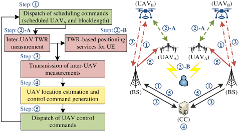
Figure 2: Structure and operation strategy of the proposed system.

Fig. 2 shows the structure and operation strategy of the proposed system. At the beginning of each time slot, the control center (CC) sends scheduling commands to all UAV_A through terrestrial BSs and ground-to-air (G2A) communication links. The scheduling commands contain the index of the UAV_A that need to perform state sensing in this time slot and the blocklength for the transmission of sensing data. Since terrestrial BSs commonly have large transmit power, the dispatch of scheduling commands is assumed to be perfect without any failure. After receiving the scheduling commands, the scheduled UAV_A cooperate with UAV_B to measure the corresponding inter-UAV distances, and send the velocity and acceleration measurements obtained by onboard sensors to UAV_B. Subsequently, UAV_A provide positioning services to UEs utilizing the two-way ranging (TWR) technique, while UAV_B transmit the sensing data obtained in the previous step to the terrestrial BSs and CC. The A2G channels between UAV_B and terrestrial BSs are modeled as Rayleigh fading channels. Due to the time-varying nature of fading channel and UAVs’ limited transmit power, failures may occur in the transmission of sensing data, which affect the state estimation and control of UAV_A. If the data required for the state sensing of a UAV_A is successfully received by BSs, CC will estimate its current state and generate the control input command based on closed-loop (CL) operation mode. Otherwise, the UAV_A will be controlled in open-loop (OP) mode based on its previously estimated states. At the end of this time slot, CC sends control commands to UAV_A, and each UAV_A adjusts its state according to the received command. Similar to scheduling commands, the dispatch of control commands is also assumed to be perfect.

With the structure and operation strategy introduced above, the proposed system is expected to work efficiently and provide positioning services that meet users’ requirements. In the following subsections, we provide the key mathematical models used in our system.

II-A Model of UAV State Sensing

In the proposed system, the true state of the $j$-th UAV_A in time slot $t$ can be represented by the following vector:

$${{\bf{x}}_{j,t}}={\left[{\Delta{\bf{q}}_{j,t}^{T},{\bf{v}}_{j,t}^{T},{\bf{a}}_{j,t}^{T}}\right]^{T}}\in{\mathbb{R}^{6\times 1}},$$ (1)

where $\Delta{{\bf{q}}_{j,t}}\!=\!{\left[{\Delta q_{j,t}^{\left(x\right)},\Delta q_{j,t}^{\left(y\right)}}\right]^{T}}\!=\!{{\bf{q}}_{j,t}}\!-\!{\bf{q}}_{j}^{\circ}$ denotes the deviation between the $j$-th UAV_A’s true location and its corresponding HP; ${{\bf{v}}_{j,t}}\!=\!{\left[{v_{j,t}^{\left(x\right)},v_{j,t}^{\left(y\right)}}\right]^{T}}\!\in\!{\mathbb{R}^{2\times 1}}$ and ${{\bf{a}}_{j,t}}\!=\!{\left[{a_{j,t}^{\left(x\right)},a_{j,t}^{\left(y\right)}}\right]^{T}}\!\in\!{\mathbb{R}^{2\times 1}}$ are the true values of the UAV_A’s velocity and acceleration, respectively. Under ideal conditions without sensing and control errors, the UAV_A should hover stably at the specified HP, i.e., ${{\bf{x}}_{j,t}}={{\bf{0}}_{6\times 1}}$.

In order to estimate the UAV_A’s location, the well-known TWR technique is used to measure the inter-UAV distances between UAV_A and UAV_B. As derived in Appendix A, the relative range measurement corresponding to the $j$-th UAV_A and $i$-th UAV_B can be expressed as

$$\hat{d}_{j,t}^{i}=d_{j,t}^{i}+n_{d,j,t}^{i}={\left\|{{\bf{q}}_{j,t}^{3D}-{\bf{b}}_{i}^{3D}}\right\|_{2}}+n_{d,j,t}^{i},$$ (2)

where $d_{j,t}^{i}={\left\|{{\bf{q}}_{j,t}^{3D}-{\bf{b}}_{i}^{3D}}\right\|_{2}}$ denotes the true distance between the $j$-th UAV_A and $i$-th UAV_B; $n_{d,j,t}^{i}\sim{\cal N}\left({0,\sigma_{d}^{2}}\right)$ is the distance measurement error caused by the clock drifts of UAVs’ local clocks, and $\sigma_{d}^{2}$ is its variance. As mentioned in [15], the value of $\sigma_{d}^{2}$ is mainly determined by the crystal tolerance of UAV’s oscillator and response delay of TWR. Since UAVs in the proposed system use the same type of oscillators and the same TWR protocol, all inter-UAV distance measurements have the same variance ($\sigma_{d}^{2}$).

For each UAV_A $j$, three UAV_B are assigned to sense its state, denoted by the set ${\cal N}_{B}^{{A_{j}}}$ (${\cal N}_{B}^{{A_{j}}}\in{{\cal N}_{B}}$). Then, the three inter-UAV distance measurements corresponding to the $j$-th UAV_A can be represented by the following vector:

$${{\bf{\hat{d}}}_{j,t}}={\left[{\cdots,\hat{d}_{j,t}^{i},\cdots}\right]^{T}}={{\bf{d}}_{j,t}}+{{\bf{n}}_{{\bf{d}},j,t}},\quad i\in{\cal N}_{B}^{{A_{j}}},$$ (3)

where ${{\bf{d}}_{j,t}}={\left[{\cdots,d_{j,t}^{i},\cdots}\right]^{T}}$ ($i\in{\cal N}_{B}^{{A_{j}}}$); ${{\bf{n}}_{{\bf{d}},j,t}}={\left[{\cdots,n_{d,j,t}^{i},\cdots}\right]^{T}}$ is the noise vector consisting of mutually independent measurement errors with same variance. Thus, the covariance matrix of ${{\bf{n}}_{{\bf{d}},j,t}}$ can be expressed as ${{\bf{R}}_{\bf{d}}}=\sigma_{d}^{2}\cdot{{\bf{I}}_{3}}$.

With the above measurement equations, the $j$-th UAV_A’s location in time slot $t$ can be estimated by CC through the maximum-likelihood (ML) method. Then, the Cramér-Rao lower bound (CRLB) that can be approached by the ML method is used to indicate the accuracy of the estimation of UAV_A’s locations, which can be expressed as

$${\mathop{\rm CRLB}\nolimits}\left({{{\bf{q}}_{j,t}}}\right)={\left({{\bf{H}}_{j}^{T}{\bf{R}}_{\bf{d}}^{-1}{{\bf{H}}_{j}}}\right)^{-1}}=\sigma_{d}^{2}\cdot{\left({{\bf{H}}_{j}^{T}{{\bf{H}}_{j}}}\right)^{-1}},$$ (4)

where ${{\bf{H}}_{j}}$ is the Jacobian matrix of equation (3) at ${{\bf{q}}_{j,t}}$, and

$${{\bf{H}}_{j}}={{\partial{{\bf{d}}_{j,t}}}\mathord{\left/{\vphantom{{\partial{{\bf{d}}_{j,t}}}{\partial{{\bf{q}}_{j,t}}}}}\right.\kern-1.2pt}{\partial{{\bf{q}}_{j,t}}}}={\left[{\cdots\!,{\bf{h}}_{j}^{i}\left({{{\bf{q}}_{j,t}}}\right),\!\cdots}\right]^{T}}={\left[{\cdots\!,{{{{\left({{{\bf{q}}_{j,t}}\!-\!{{\bf{b}}_{i}}}\right)}\mathord{\left/{\vphantom{{\left({{{\bf{q}}_{j,t}}-{{\bf{b}}_{i}}}\right)}{\left\|{{\bf{q}}_{j,t}^{3D}\!-\!{\bf{b}}_{i}^{3D}}\right\|}}}\right.\kern-1.2pt}{\left\|{{\bf{q}}_{j,t}^{3D}-{\bf{b}}_{i}^{3D}}\right\|}}}_{2}},\!\cdots}\right]^{T}},\;i\in{\cal N}_{B}^{{A_{j}}}.$$ (5)

It is noteworthy that with appropriate control strategy, the deviation between UAV_A’s true location (${{\bf{q}}_{j,t}}$) and the corresponding HP (${\bf{q}}_{j}^{\circ}$) is acceptable, and its influence on the geometry of UAVs is negligible [25, 35]. Thus, by replacing ${{\bf{q}}_{j,t}}$ in equation (5) with ${\bf{q}}_{j}^{\circ}$, ${{\bf{H}}_{j}}$ can be approximated as

$${{\bf{H}}_{j}}\approx{\left[{\cdots\!,{\bf{h}}_{j}^{i}\left({{\bf{q}}_{j}^{\circ}}\right),\!\cdots}\right]^{T}}={\left[{\cdots\!,{{\left({{\bf{q}}_{j}^{\circ}-{{\bf{b}}_{i}}}\right)}\mathord{\left/{\vphantom{{\left({{\bf{q}}_{j}^{\circ}-{{\bf{b}}_{i}}}\right)}{{{\left\|{{\bf{q}}_{j}^{\circ,3D}\!-\!{\bf{b}}_{i}^{3D}}\right\|}_{2}}}}}\right.\kern-1.2pt}{{{\left\|{{\bf{q}}_{j}^{\circ,3D}\!-\!{\bf{b}}_{i}^{3D}}\right\|}_{2}}}},\!\cdots}\right]^{T}}.$$ (6)

We assume that the estimation of UAV_A’s location performed at CC could approach the CRLB. Then, the covariance matrix of UAV_A location estimate (${{\bf{\hat{q}}}_{j,t}}$) can be expressed as ${{\bf{R}}_{{\bf{q}},j}}\approx{\mathop{\rm CRLB}\nolimits}\left({{{\bf{q}}_{j,t}}}\right)$. Moreover, utilizing the relationship $\Delta{{\bf{q}}_{j,t}}={{\bf{q}}_{j,t}}-{\bf{q}}_{j}^{\circ}$, the estimate of $\Delta{{\bf{q}}_{j,t}}$ can be written as

$$\Delta{{\bf{\hat{q}}}_{j,t}}={{\bf{\hat{q}}}_{j,t}}-{\bf{q}}_{j}^{\circ}=\Delta{{\bf{q}}_{j,t}}+{{\bf{n}}_{\Delta{\bf{q}},j,t}},$$ (7)

where ${{\bf{n}}_{\Delta{\bf{q}},j,t}}\sim{\cal N}\left({{{\bf{0}}_{2\times 1}},{{\bf{R}}_{\Delta{\bf{q}},j}}}\right)$ is the location estimation error, and ${{\bf{R}}_{\Delta{\bf{q}},j}}={{\bf{R}}_{{\bf{q}},j}}$ is its covariance matrix.

In addition, while measuring the inter-UAV distances, UAV_A also send their velocity and acceleration measurements to UAV_B by embedding them into the response message of TWR. The velocity and acceleration of the $j$-th UAV_A measured in time slot $t$ can be expressed as

$${{\bf{\hat{v}}}_{j,t}}={{\bf{v}}_{j,t}}+{{\bf{n}}_{{\bf{v}},j,t}},\qquad\qquad{{\bf{\hat{a}}}_{j,t}}={{\bf{a}}_{j,t}}+{{\bf{n}}_{{\bf{a}},j,t}},$$ (8)

where ${{\bf{n}}_{{\bf{v}},j,t}}\sim{\cal N}\left({{{\bf{0}}_{2\times 1}},{{\bf{R}}_{\bf{v}}}}\right)$ and ${{\bf{n}}_{{\bf{a}},j,t}}\sim{\cal N}\left({{{\bf{0}}_{2\times 1}},{{\bf{R}}_{\bf{a}}}}\right)$ represent measurement errors. Since we assume that all UAV_A are equipped with the same sensors, the velocity (acceleration) measurements in the proposed system have the same covariance matrix ${{\bf{R}}_{\bf{v}}}$ (${{\bf{R}}_{\bf{a}}}$).

Then, the sensing results of the $j$-th UAV_A’s state in time slot $t$ can be represented by the following vector:

$${{\bf{\hat{x}}}_{j,t}}={\left[{\Delta{\bf{\hat{q}}}_{j,t}^{T},{\bf{\hat{v}}}_{j,t}^{T},{\bf{\hat{a}}}_{j,t}^{T}}\right]^{T}}={{\bf{x}}_{j,t}}+{{\bm{\eta}}_{j,t}},$$ (9)

where ${{\bm{\eta}}_{j,t}}={\left[{{{\bf{n}}_{\Delta{\bf{q}},j,t}},{{\bf{n}}_{{\bf{v}},j,t}},{{\bf{n}}_{{\bf{a}},j,t}}}\right]^{T}}\sim{\cal N}\left({{{\bf{0}}_{6\times 1}},{{\bf{R}}_{{\bm{\eta}},j}}}\right)$ is the noise vector consisting of three kinds of mutually independent measurement errors, and its covariance matrix can be written as

$${{\bf{R}}_{\bm{\eta},j}}={\rm blkdiag}\left({{{\bf{R}}_{\Delta{\bf{q}},j}},{{\bf{R}}_{\bf{v}}},{{\bf{R}}_{\bf{a}}}}\right).$$ (10)

II-B Model of UAV Control

For simplicity and without loss of generality, we model each UAV_A in the proposed system as a linear time-invariant discrete-time system, whose dynamics model is given by

$${{\bf{x}}_{j,t+1}}={{\bf{A}}_{j}}{{\bf{x}}_{j,t}}+{{\bf{B}}_{j}}{{\bf{u}}_{j,t}}+{{\bf{w}}_{j,t}},$$ (11)

where ${{\bf{A}}_{j}}\in{\mathbb{R}^{6\times 6}}$ and ${{\bf{B}}_{j}}\in{\mathbb{R}^{6\times 2}}$ are the state matrix and input matrix of the $j$-th UAV_A, respectively; ${{\bf{u}}_{j,t}}={\left[{u_{j}^{\left(x\right)},u_{j}^{\left(y\right)}}\right]^{T}}\in{\mathbb{R}^{2\times 1}}$ is the control input, i.e., the commanded acceleration; ${{\bf{w}}_{j,t}}\sim{\cal N}\left({{{\bf{0}}_{6\times 1}},{{\bf{Q}}_{\bf{w}}}}\right)$ is independent identically distributed (i.i.d.) process noise that characterizes the unintentional movements of UAV_A. The expressions for matrices ${{\bf{A}}_{j}}$, ${{\bf{B}}_{j}}$ and ${{\bf{Q}}_{\bf{w}}}$ are derived in Appendix B.

As a linear system, UAV_A’s control input vector can be determined using the state feedback law ${{\bf{u}}_{j,t}}={{\bf{K}}_{j}}{{\bf{x}}_{j,t}}$, where ${{\bf{K}}_{j}}\in{\mathbb{R}^{2\times 6}}$ is the gain matrix. Then, equation (11) can be rewritten as

$${{\bf{x}}_{j,t+1}}=\left({{{\bf{A}}_{j}}+{{\bf{B}}_{j}}{{\bf{K}}_{j}}}\right){{\bf{x}}_{j,t}}+{{\bf{w}}_{j,t}}.$$ (12)

Please note that the true state (${{\bf{x}}_{j,t}}$) in the above equation is unavailable in practice. Therefore, CC can only generate the control input (${{\bf{u}}_{j,t}}$) based on state sensing or prediction results. If the sensing data is successfully received by CC, the control input will be generated in CL mode based on the estimated state (${{\bf{\hat{x}}}_{j,t}}$), i.e., ${\bf{u}}_{j,t}^{\left(c\right)}={{\bf{K}}_{j}}{{\bf{\hat{x}}}_{j,t}}={{\bf{K}}_{j}}\left({{{\bf{x}}_{j,t}}+{{\bm{\eta}}_{j,t}}}\right)$. Otherwise, the UAV_A will be controlled in OL mode and the control input is generated based on the predicted state. According to equation (12), if the last successful state sensing was performed in time slot $t-\Delta t_{j}^{c}$, the prediction of UAV_A’s state in time slot $t$ can be expressed as

$${\bf{\bar{x}}}_{j,t}^{\left({\Delta t_{j}^{c}}\right)}={\left({{{\bf{A}}_{j}}+{{\bf{B}}_{j}}{{\bf{K}}_{j}}}\right)^{\Delta t_{j}^{c}}}{{{\bf{\hat{x}}}}_{j,t-\Delta t_{j}^{c}}}={\left({{{\bf{A}}_{j}}\!+\!{{\bf{B}}_{j}}{{\bf{K}}_{j}}}\right)^{\Delta t_{j}^{c}}}\left({{{\bf{x}}_{j,t-\Delta t_{j}^{c}}}\!+\!{{\bm{\eta}}_{j,t-\Delta t_{j}^{c}}}}\right).$$ (13)

Then, the control input generated in OL mode can be written as ${\bf{u}}_{j,t}^{\left(o\right)}={{\bf{K}}_{j}}{\bf{\bar{x}}}_{j,t}^{\left({\Delta t_{j}^{c}}\right)}$, and the UAV_A’s dynamics model in two operation modes can be expressed as

$$\begin{split}{\bf{x}}_{j,t+1}^{\left(c\right)}&=\left({{{\bf{A}}_{j}}+{{\bf{B}}_{j}}{{\bf{K}}_{j}}}\right){{\bf{x}}_{j,t}}+\left({{{\bf{B}}_{j}}{{\bf{K}}_{j}}{{\bm{\eta}}_{j,t}}+{{\bf{w}}_{j,t}}}\right),\quad{\rm closed\raisebox{0.0pt}{-}loop},\\ {\bf{x}}_{j,t+1}^{\left(o\right)}&={{\bf{A}}_{j}}{{\bf{x}}_{j,t}}+{{\bf{B}}_{j}}{{\bf{K}}_{j}}{\bf{\bar{x}}}_{j,t}^{\left({\Delta t_{j}^{c}}\right)}+{{\bf{w}}_{j,t}},\qquad\qquad\quad\;{\rm open\raisebox{0.0pt}{-}loop},\end{split}$$ (14)

where superscripts $\left(c\right)$ and $\left(o\right)$ indicate the CL and OL modes, respectively.

Furthermore, the update rule for parameter $\Delta t_{j}^{c}$ in two operation modes is given by

$$\Delta t_{j}^{c}\leftarrow\left\{{\begin{array}[]{*{20}{c}}{1,\qquad\qquad{\rm closed\raisebox{0.0pt}{-}loop},}\\ {\Delta t_{j}^{c}+1,\quad\;\,{\rm open\raisebox{0.0pt}{-}loop}.}\end{array}}\right.$$ (15)

II-C Model of Positioning Services for UE

As mentioned at the beginning of this section, in the proposed system, UAV_A are employed as aerial anchor nodes to provide TWR-based positioning services for UEs. Similar to the measurement of inter-UAV distances, the distance measurement between the $m$-th UE and $j$-th UAV_A obtained through the TWR technique in time slot $t$ can be expressed as

$$\hat{r}_{m,t}^{j}=r_{m,t}^{j}+n_{r,m,t}^{j}={\left\|{{\bf{p}}_{m}^{3D}-{\bf{q}}_{j,t}^{3D}}\right\|_{2}}+n_{r,m,t}^{j},$$ (16)

where $r_{m,t}^{j}={\left\|{{\bf{p}}_{m}^{3D}-{\bf{q}}_{j,t}^{3D}}\right\|_{2}}$ denotes the true distance; $n_{r,m,t}^{j}\sim{\cal N}\left({0,\sigma_{r}^{2}}\right)$ is the i.i.d. measurement error, and $\sigma_{r}^{2}$ is its variance.

Denote the $N_{A}^{U}$ UAV_A ($N_{A}^{U}\geq 3$) serving the $m$-th UE as the set ${\cal N}_{A}^{{U_{m}}}$ (${\cal N}_{A}^{{U_{m}}}\in{{\cal N}_{A}}$), then the distance measurements available to the UE form the following vector:

$${{\bf{\hat{r}}}_{m,t}}={\left[{\cdots,\hat{r}_{m,t}^{j},\cdots}\right]^{T}}={{\bf{r}}_{m,t}}+{{\bf{n}}_{{\bf{r}},m,t}},\quad j\in{\cal N}_{A}^{{U_{m}}},$$ (17)

where ${{\bf{r}}_{m,t}}={\left[{\cdots,r_{m,t}^{j},\cdots}\right]^{T}}$ ($j\in{\cal N}_{A}^{{U_{m}}}$); ${{\bf{n}}_{{\bf{r}},m,t}}={\left[{\cdots,n_{r,m,t}^{j},\cdots}\right]^{T}}$ is the noise vector consisting of $N_{A}^{U}$ i.i.d. measurement errors, and its covariance matrix can be written as ${{\bf{R}}_{\bf{r}}}=\sigma_{r}^{2}\cdot{{\bf{I}}_{N_{A}^{U}}}$.

Due to unknown sensing and control errors, the true locations of UAV_A are time-varying and unavailable to UEs. Thus, UEs can only use UAV_A’s HPs and the following measurement equations for position estimation:

$${{{\bf{\bar{r}}}}_{m}}\left({{{\bf{p}}_{m}}}\right)={\left[{\cdots,\bar{r}_{m}^{j}\left({{{\bf{p}}_{m}}}\right),\cdots}\right]^{T}}={\left[{\cdots,{{\left\|{{\bf{p}}_{m}^{3D}-{\bf{q}}_{j}^{\circ,3D}}\right\|}_{2}},\cdots}\right]^{T}}.$$ (18)

In this article, the iterative least-squares (ILS) method that estimates unknown parameters in an iterative manner through Taylor-series linearization is used to determine UEs’ locations [36]. Denote the $m$-th UE’s location estimate obtained in the $l$-th iteration of ILS as ${\bf{\hat{p}}}_{m,t}^{\left(l\right)}\in{\mathbb{R}^{2\times 1}}$ (${\bf{\hat{p}}}_{m,t}^{\left(l\right),3D}={\left[{{{\left({{\bf{\hat{p}}}_{m,t}^{\left(l\right)}}\right)}^{T}},0}\right]^{T}}$), then the first-order Taylor-series expansion of ${{\bf{\bar{r}}}_{m}}\left({{{\bf{p}}_{m}}}\right)$ at ${\bf{\hat{p}}}_{m,t}^{\left(l\right)}$ can be written as

$${{\bf{\bar{r}}}_{m}}\left({{{\bf{p}}_{m}}}\right)\simeq{{\bf{\bar{r}}}_{m}}\left({{\bf{\hat{p}}}_{m,t}^{\left(l\right)}}\right)+{{\bf{H}}_{m}}\left({{\bf{\hat{p}}}_{m,t}^{\left(l\right)}}\right)\left({{{\bf{p}}_{m}}-{\bf{\hat{p}}}_{m,t}^{\left(l\right)}}\right),$$ (19)

where

$${{\bf{H}}_{m}}\left(\!{{\bf{\hat{p}}}_{m,t}^{\left(l\right)}}\!\right)={\left.{\frac{{\partial{{{\bf{\bar{r}}}}_{m}}\left({{{\bf{p}}_{m}}}\right)}}{{\partial{{\bf{p}}_{m}}}}}\right|_{{\bf{\hat{p}}}_{m,t}^{\left(l\right)}}}\!=\!{\left[{\cdots,{\bf{h}}_{m}^{j}\left(\!{{\bf{\hat{p}}}_{m,t}^{\left(l\right)}}\!\right),\cdots}\right]^{T}}={\left[{\cdots,\frac{{\left({{\bf{\hat{p}}}_{m,t}^{\left(l\right)}\!-\!{\bf{q}}_{j}^{\circ}}\right)}}{{{{\left\|{{\bf{\hat{p}}}_{m,t}^{\left(l\right),3D}\!-\!{\bf{q}}_{j}^{\circ,3D}}\right\|}_{2}}}},\cdots}\right]^{T}}$$ (20)

is the Jacobian matrix of equation (18) at ${\bf{\hat{p}}}_{m,t}^{\left(l\right)}$.

The LS estimate of the $m$-th UE’s location obtained in the $\left({l+1}\right)$-th iteration is given by

$${\bf{\hat{p}}}_{m,t}^{\left({l+1}\right)}={\bf{\hat{p}}}_{m,t}^{\left(l\right)}+{\bf{S}}\left({{\bf{\hat{p}}}_{m,t}^{\left(l\right)}}\right)\left[{{{{\bf{\hat{r}}}}_{m,t}}-{{{\bf{\bar{r}}}}_{m}}\left({{\bf{\hat{p}}}_{m,t}^{\left(l\right)}}\right)}\right],$$ (21)

where

$${\bf{S}}\left({{\bf{\hat{p}}}_{m,t}^{\left(l\right)}}\right)={\bf{P}}\left({{\bf{\hat{p}}}_{m,t}^{\left(l\right)}}\right){\bf{H}}{\left({{\bf{\hat{p}}}_{m,t}^{\left(l\right)}}\right)^{T}},$$ (22)

$${\bf{P}}\left({{\bf{\hat{p}}}_{m,t}^{\left(l\right)}}\right)={\left[{{\bf{H}}{{\left({{\bf{\hat{p}}}_{m,t}^{\left(l\right)}}\right)}^{T}}{\bf{H}}\left({{\bf{\hat{p}}}_{m,t}^{\left(l\right)}}\right)}\right]^{-1}}.$$ (23)

The estimation result of the $m$-th UE’s location in time slot $t$ can be obtained after the above iteration converges.

III Performance Analysis and Problem Formulation

In this article, the UAV position uncertainty caused by sensing and control errors is taken into account in the design of our UAV-enabled positioning system, which has often been overlooked in existing research. Due to this additional consideration, the analysis methods and performance metrics used in previous research are unsuitable for evaluating the performance of the proposed system. Therefore, in the first two subsections of this section, we first analysis the stability of UAV_A in two operation modes, and then derive the MSE of UE positioning in the presence of UAV position uncertainty. It is found that the scheduling of UAV_A state sensing and the blocklength for the transmission of sensing data are two main factors affecting the quality of positioning services. Thus, at the end of this section, we formulate the sensing scheduling and blocklength allocation in the proposed system as a QoS-constrained optimization problem, which will be solved using the scheme introduced in the next section.

III-A UAV Stability Prediction in Different Operation Modes

The aim of this subsection is to predict the stability of each UAV_A in the next time slot ($t+1$) before CC generates the scheduling commands for the current time slot ($t$). The UAV_A’s dynamics model in two operation modes has been derived in Section II.B. However, it is noteworthy that the dynamics model shown in equation (14) uses the true state of UAV_A (${{\bf{x}}_{j,t}}$) when calculating its future state, which is unknown in practice. Therefore, in order to predict UAV_A’s state in time slot $t+1$, we need to replace ${{\bf{x}}_{j,t}}$ in equation (14) with other variables whose values or distributions are available to CC. We assume that the last successful state sensing was performed $t+1$ time slots ago. Then, according to equations (13) and (14), the expression for ${{\bf{x}}_{j,t}}$ can be written as

$${{\bf{x}}_{j,t}}\!=\!{\left(\!{{{\bf{A}}\!_{j}}\!+\!{{\bf{B}}\!_{j}}{{\bf{K}}\!_{j}}}\!\right)^{\Delta t_{j}^{c}}}{{\bf{x}}_{j,t-\Delta t_{j}^{c}}}+\left[\!{\sum\limits_{k=0}^{\Delta t_{j}^{c}\!-\!1}\!{{\bf{A}}\!_{j}^{k}{{\bf{B}}\!_{j}}{{\bf{K}}\!_{j}}{{\left(\!{{{\bf{A}}\!_{j}}\!+\!{{\bf{B}}\!_{j}}{{\bf{K}}\!_{j}}}\!\right)}^{\Delta t_{j}^{c}\!-\!k\!-\!1}}}}\!\right]\!{{\bm{\eta}}_{j,t\!-\!\Delta t_{j}^{c}}}\!+\!\sum\limits_{k=0}^{\Delta t_{j}^{c}-1}\!{{\bf{A}}\!_{j}^{k}{{\bf{w}}_{j,t-k-1}}}.$$ (24)

Moreover, utilizing the relationship ${{\bf{x}}_{j,t-\Delta t_{j}^{c}}}={{\bf{\hat{x}}}_{j,t-\Delta t_{j}^{c}}}-{{\bm{\eta}}_{j,t-\Delta t_{j}^{c}}}$ and equation (13), the above equation can be further rewritten as

$${{\bf{x}}_{j,t}}\!=\!{\bf{\bar{x}}}_{j,t}^{\left(\!{\Delta t_{j}^{c}}\!\right)}\!+\!\left[\!{\left(\!{\sum\limits_{k=0}^{\Delta t_{j}^{c}\!-\!1}\!{{\bf{A}}\!_{j}^{k}{{\bf{B}}_{j}}{{\bf{K}}_{j}}{{\left(\!{{{\bf{A}}\!_{j}}\!+\!{{\bf{B}}_{j}}{{\bf{K}}_{j}}}\!\right)}\!^{\Delta t_{j}^{c}\!-\!k\!-\!1}}}}\!\right)\!-\!{{\left(\!{{{\bf{A}}\!_{j}}\!+\!{{\bf{B}}_{j}}{{\bf{K}}_{j}}}\!\right)}\!^{\Delta t_{j}^{c}}}}\!\right]\!{{\bm{\eta}}_{j,t\!-\!\Delta t_{j}^{c}}}\!+\!\sum\limits_{k=0}^{\Delta t_{j}^{c}\!-\!1}\!{{\bf{A}}\!_{j}^{k}{{\bf{w}}_{j,t\!-\!k\!-\!1}}}.$$ (25)

The value of ${\bf{\bar{x}}}_{j,t}^{\left({\Delta t_{j}^{c}}\right)}$ in the above equation can be calculated using equation (13), and the distributions of noise vectors ${{\bm{\eta}}_{j,t-\Delta t_{j}^{c}}}$ and ${{\bf{w}}_{j,t-k-1}}$ are known. Then, by substituting this equation into equation (14), the UAV_A’s dynamics model in two operation modes can be rewritten as

$$\begin{split}{\bf{x}}\!_{j,t\!+\!1}^{\left(c\right)}&\!=\!{\bf{A}}\!_{j}^{\left(\!c\!\right)}{\bf{\bar{x}}}\!_{j,t}^{\left(\!{\Delta t_{j}^{c}}\!\right)}\!+\!\left(\!{{\bf{A}}\!_{j}^{\left(\!c\!\right)}\!{\bf{C}}\!_{j}^{\left(\!{\Delta t_{j}^{c}}\!\right)}\!{{\bm{\eta}}_{j,t\!-\!\Delta t_{j}^{c}}}\!+\!{{\bf{B}}\!_{j}}{{\bf{K}}\!_{j}}{{\bm{\eta}}_{j,t}}}\!\right)\!+\!\left(\!{\sum\limits_{k=0}^{\Delta t_{j}^{c}\!-\!1}\!{{\bf{A}}\!_{j}^{\left(\!c\!\right)}\!{\bf{A}}\!_{j}^{k}{{\bf{w}}\!_{j,t\!-\!k\!-\!1}}}\!+\!{{\bf{w}}\!_{j,t}}}\!\right)\!,{\rm closed\raisebox{0.0pt}{-}loop},\\ {\bf{x}}_{j,t\!+\!1}^{\left(o\right)}&\!=\!{\bf{A}}\!_{j}^{\left(\!c\!\right)}{\bf{\bar{x}}}_{j,t}^{\left(\!{\Delta t_{j}^{c}}\!\right)}\!+\!{{\bf{A}}\!_{j}}{\bf{C}}\!_{j}^{\left(\!{\Delta t_{j}^{c}}\!\right)}{{\bm{\eta}}_{j,t\!-\!\Delta t_{j}^{c}}}\!+\!\sum\limits_{k=0}^{\Delta t_{j}^{c}}\!{{\bf{A}}\!_{j}^{k}{{\bf{w}}\!_{j,t\!-\!k}}},\qquad\qquad\qquad\qquad\qquad\quad\;{\rm open\raisebox{0.0pt}{-}loop},\end{split}$$ (26)

where

$${\bf{A}}_{j}^{\left(c\right)}={{\bf{A}}_{j}}+{{\bf{B}}_{j}}{{\bf{K}}_{j}}$$ (27)

is the closed loop state matrix, and

$${\bf{C}}_{j}^{\left({\Delta t_{j}^{c}}\right)}=\left[{\sum\limits_{k=0}^{\Delta t_{j}^{c}-1}{{\bf{A}}_{j}^{k}{{\bf{B}}_{j}}{{\bf{K}}_{j}}{{\left({{\bf{A}}_{j}^{\left(c\!\right)}}\right)}^{\Delta t_{j}^{c}-k-1}}}-{{\left(\!{{\bf{A}}_{j}^{\left(c\right)}}\right)}^{\Delta t_{j}^{c}}}}\right].$$ (28)

Please note that the values of vectors ${{\bm{\eta}}_{j,t-\Delta t_{j}^{c}}}$ and ${{\bf{w}}_{j,t-k-1}}$ in equation (26) are unavailable. Therefore, we choose to predict the covariance matrix of UAV_A’s state in time slot $t$ instead of its true value. According to equation (26), the predicted covariance matrix in two operation modes can be expressed as

$$\begin{split}{\bf{Q}}_{{\bf{x}},j,t\!+\!1}^{\left(c\right)}&\!=\!E\!\left\{\!{\left(\!{{\bf{x}}\!_{j,t\!+\!1}^{\left(c\right)}}\!\right)\!{{\left(\!{{\bf{x}}_{j,t\!+\!1}^{\left(c\right)}}\!\right)}^{T}}}\!\right\}\!=\!\left(\!{{\bf{A}}\!_{j}^{\left(\!c\!\right)}{\bf{\bar{x}}}_{j,t}^{\left(\!{\Delta t_{j}^{c}}\!\right)}}\!\right)\!{\left(\!{{\bf{A}}\!_{j}^{\left(\!c\!\right)}{\bf{\bar{x}}}_{j,t}^{\left(\!{\Delta t_{j}^{c}}\!\right)}}\!\right)^{T}}\!+\!\left(\!{{\bf{A}}\!_{j}^{\left(\!c\!\right)}{\bf{C}}_{j}^{\left(\!{\Delta t_{j}^{c}}\!\right)}}\!\right)\!{{\bf{R}}_{\bm{\eta},j}}\!{\left(\!{{\bf{A}}\!_{j}^{\left(\!c\!\right)}{\bf{C}}_{j}^{\left(\!{\Delta t_{j}^{c}}\!\right)}}\!\right)^{T}}\\ &\qquad\qquad\qquad\qquad\quad\;+\left({{{\bf{B}}_{j}}{{\bf{K}}_{j}}}\right)\!{{\bf{R}}_{\bm{\eta},j}}{\left({{{\bf{B}}_{j}}{{\bf{K}}_{j}}}\right)^{T}}\!+\!\sum\limits_{k=0}^{\Delta t_{j}^{c}\!-\!1}\!{\left(\!{{\bf{A}}\!_{j}^{\left(\!c\!\right)}{\bf{A}}\!_{j}^{k}}\right)\!{{\bf{Q}}_{\bf{w}}}\!{{\left(\!{{\bf{A}}\!_{j}^{\left(\!c\!\right)}{\bf{A}}\!_{j}^{k}}\!\right)}^{T}}}\!+\!{{\bf{Q}}_{\bf{w}}},\\ {\bf{Q}}_{{\bf{x}},j,t\!+\!1}^{\left(o\right)}&\!=\!E\!\left\{\!{\left(\!{{\bf{x}}_{j,t\!+\!1}^{\left(o\right)}}\!\right)\!{{\left(\!{{\bf{x}}_{j,t\!+\!1}^{\left(o\right)}}\!\right)}^{T}}}\!\right\}\!=\!\left(\!{{\bf{A}}\!_{j}^{\left(\!c\!\right)}{\bf{\bar{x}}}_{j,t}^{\left(\!{\Delta t_{j}^{c}}\!\right)}}\!\right)\!{\left(\!{{\bf{A}}\!_{j}^{\left(\!c\!\right)}{\bf{\bar{x}}}_{j,t}^{\left(\!{\Delta t_{j}^{c}}\!\right)}}\!\right)^{T}}\!+\!\left(\!{{{\bf{A}}\!_{j}}{\bf{C}}_{j}^{\left(\!{\Delta t_{j}^{c}}\!\right)}}\!\right)\!{{\bf{R}}_{\bm{\eta},j}}\!{\left(\!{{{\bf{A}}\!_{j}}{\bf{C}}_{j}^{\left(\!{\Delta t_{j}^{c}}\!\right)}}\!\right)^{T}}\\ &\qquad\qquad\qquad\qquad\quad\;+\sum\limits_{k=0}^{\Delta t_{j}^{c}}\!{\left({{\bf{A}}\!_{j}^{k}}\right)\!{{\bf{Q}}_{\bf{w}}}\!{{\left({{\bf{A}}\!_{j}^{k}}\right)}^{T}}.}\end{split}$$ (29)

In this article, we mainly focus on the UAV position uncertainty ($\Delta{{\bf{q}}_{j,t+1}}={\left({{{\bf{x}}_{j,t+1}}}\right)_{1:2}}$), whose covariance matrix can be written as

$$\begin{split}{\bf{Q}}_{\Delta{\bf{q}},j,t+1}^{\left(c\right)}&={\left({{\bf{Q}}_{{\bf{x}},j,t+1}^{\left(c\right)}}\right)_{2\times 2}},\quad\;{\rm closed\raisebox{0.0pt}{-}loop},\\ {\bf{Q}}_{\Delta{\bf{q}},j,t+1}^{\left(o\right)}&={\left({{\bf{Q}}_{{\bf{x}},j,t+1}^{\left(o\right)}}\right)_{2\times 2}},\quad\;{\rm open\raisebox{0.0pt}{-}loop}.\end{split}$$ (30)

III-B UE Positioning Performance with UAV Control Error

The covariance matrix of UAV position uncertainty has been derived in the previous subsection. Then, in this subsection, we further analyze the performance of positioning services in the presence of UAV control error. According to the model described in Section II.C, the estimation error of the $m$-th UE’s location in the $\left({l+1}\right)$-th iteration of ILS can be expressed as

$$\Delta{\bf{p}}_{m,t+1}^{\left({l+1}\right)}={\bf{\hat{p}}}_{m,t+1}^{\left({l+1}\right)}-{{\bf{p}}_{m}}=\left({{\bf{\hat{p}}}_{m,t+1}^{\left(l\right)}-{{\bf{p}}_{m}}}\right)+{\bf{S}}\left({{\bf{\hat{p}}}_{m,t+1}^{\left(l\right)}}\right)\left[{{{{\bf{\hat{r}}}}_{m,t+1}}-{{{\bf{\bar{r}}}}_{m}}\left({{\bf{\hat{p}}}_{m,t+1}^{\left(l\right)}}\right)}\right].$$ (31)

With appropriate UAV control strategy and good initial guesses for ILS, the location estimate will be close to the true location after several iterations [25]. Thus, by replacing ${\bf{\hat{p}}}_{m,t+1}^{\left(l\right)}$ in the above equation with the true location (${{\bf{p}}_{m}}$), the estimation error of the ILS method after convergence can be written as

$$\Delta{{\bf{p}}_{m,t+1}}={{\bf{\hat{p}}}_{m,t+1}}-{{\bf{p}}_{m}}={\bf{S}}\left({{{\bf{p}}_{m}}}\right)\left[{{{{\bf{\hat{r}}}}_{m,t+1}}-{{{\bf{\bar{r}}}}_{m}}\left({{{\bf{p}}_{m}}}\right)}\right].$$ (32)

The matrix ${\bf{S}}\left({{{\bf{p}}_{m}}}\right)$ in the above equation can be easily calculated using equations (22) and (23). We then derive the expression for term $\left[{{{{\bf{\hat{r}}}}_{m,t+1}}-{{{\bf{\bar{r}}}}_{m}}\left({{{\bf{p}}_{m}}}\right)}\right]$. Applying the first-order Taylor-series expansion to equation (16) based on the relationship ${{\bf{q}}_{j,t+1}}={\bf{q}}_{j}^{\circ}+\Delta{{\bf{q}}_{j,t+1}}$ (${\bf{q}}_{j,t+1}^{3D}={\bf{q}}_{j}^{\circ,3D}+{\left[{\Delta{\bf{q}}_{j,t+1}^{T},0}\right]^{T}}$), $\hat{r}_{m,t+1}^{j}$ can be approximated as

$$\hat{r}_{m,t\!+\!1}^{j}\!\simeq\!{\left\|{{\bf{p}}_{m}^{3D}\!-\!{\bf{q}}_{j}^{\circ,3D}}\right\|_{2}}\!-{\bf{h}}_{m}^{j}{\left({{{\bf{p}}_{m}}}\right)^{T}}\Delta{{\bf{q}}_{j,t\!+\!1}}+n_{r,m,t\!+\!1}^{j}\!=\!\bar{r}_{m}^{j}\left({{{\bf{p}}_{m}}}\right)-{\bf{h}}_{m}^{j}{\left({{{\bf{p}}_{m}}}\right)^{T}}\Delta{{\bf{q}}_{j,t\!+\!1}}+n_{r,m,t\!+\!1}^{j}.$$ (33)

Then, term $\left[{{{{\bf{\hat{r}}}}_{m,t+1}}-{{{\bf{\bar{r}}}}_{m}}\left({{{\bf{p}}_{m}}}\right)}\right]$ can be rewritten as

$${{{\bf{\hat{r}}}}_{m,t\!+\!1}}-{{{\bf{\bar{r}}}}_{m}}\left({{{\bf{p}}_{m}}}\right)=-\!{\left[{\cdots\!,{\bf{h}}_{m}^{j}{{\left({{{\bf{p}}_{m}}}\right)}^{T}}\Delta{{\bf{q}}_{j,t\!+\!1}},\!\cdots}\right]^{T}}+{\left[{\cdots\!,n_{r,m,t\!+\!1}^{j},\!\cdots}\right]^{T}}\!=\!-{{\bm{\beta}}_{m,t\!+\!1}}+{{\bf{n}}_{{\bf{r}},m,t\!+\!1}}.$$ (34)

where ${{\bm{\beta}}_{m,t+1}}={\left[{\cdots,{\bf{h}}_{m}^{j}{{\left({{{\bf{p}}_{m}}}\right)}^{T}}\Delta{{\bf{q}}_{j,t+1}},\cdots}\right]^{T}}$.

Substituting the above equation into equation (32), the covariance matrix of the $m$-th UE’s position error in time slot $t+1$ can be expressed as

$$\begin{split}{\bf{Q}}_{\Delta{\bf{p}},m,t\!+\!1}^{\left({{{\bm{\xi}}_{m,t}}}\right)}&=\!E\!\left\{\!{\Delta{{\bf{p}}_{m,t\!+\!1}}\Delta{\bf{p}}_{m,t\!+\!1}^{T}}\!\right\}\!=\!E\!\left\{\!{{\bf{S}}\!\left(\!{{{\bf{p}}_{m}}}\!\right)\left(\!{-\!{{\bm{\beta}}_{m,t\!+\!1}}\!+\!{{\bf{n}}_{{\bf{r}},m,t\!+\!1}}}\!\right)\!{{\left(\!{-\!{{\bm{\beta}}_{m,t\!+\!1}}\!+\!{{\bf{n}}_{{\bf{r}},m,t\!+\!1}}}\!\right)}^{T}}\!{\bf{S}}{{\left(\!{{{\bf{p}}_{m}}}\right)}^{T}}}\!\right\}\\ &=\!{\bf{S}}\!\left(\!{{{\bf{p}}_{m}}}\!\right)\left[{E\left\{{{{\bm{\beta}}_{m,t\!+\!1}}{\bm{\beta}}_{m,t\!+\!1}^{T}}\right\}+E\left\{{{{\bf{n}}_{{\bf{r}},m,t\!+\!1}}{\bf{n}}_{{\bf{r}},m,t\!+\!1}^{T}}\right\}}\right]{\bf{S}}{\left(\!{{{\bf{p}}_{m}}}\!\right)^{T}}\\ &=\!\sigma_{r}^{2}{\bf{P}}\!\left(\!{{{\bf{p}}_{m}}}\!\right)+{\bf{S}}\!\left(\!{{{\bf{p}}_{m}}}\!\right){\mathop{\rm diag}\nolimits}\left({\ldots,{\bf{h}}_{m}^{j}{{\left({{{\bf{p}}_{m}}}\right)}^{T}}{\bf{Q}}_{\Delta{\bf{q}},j,t\!+\!1}^{\left({{\xi_{m,j,t}}}\right)}{\bf{h}}_{m}^{j}\left({{{\bf{p}}_{m}}}\right),\ldots}\right){\bf{S}}{\left(\!{{{\bf{p}}_{m}}}\!\right)^{T}},\end{split}$$ (35)

where vector ${{\bm{\xi}}_{m,t}}={\left[{\cdots,{\xi_{m,j,t}},\cdots}\right]^{T}}$ ($j\in{\cal N}_{A}^{{U_{m}}}$) represents the operation modes of the $N_{A}^{U}$ UAV_A serving the $m$-th UE; ${\xi_{m,j,t}}$ could be either $c$ or $o$, indicating the operation mode of the $j$-th UAV_A in time slot $t$; Covariance matrix ${\bf{Q}}_{\Delta{\bf{q}},j,t+1}^{\left({{\xi_{m,j,t}}}\right)}$ can be calculated using equations (29) and (30).

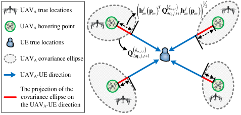
Figure 3: Explanation of UAV control errors’ impact on UE positioning.

As can be seen from equation (35), the covariance matrix of UE position error can be written as the sum of two terms. The first term $\sigma_{r}^{2}{\bf{P}}\left({{{\bf{p}}_{m}}}\right)$ denotes the position error caused by distance measurement errors, reflecting the positioning accuracy in the absence of UAV position uncertainty. The second term ${\bf{S}}\left({{{\bf{p}}_{m}}}\right){\mathop{\rm diag}\nolimits}\left({\ldots,{\bf{h}}_{m}^{j}{{\left({{{\bf{p}}_{m}}}\right)}^{T}}{\bf{Q}}_{\Delta{\bf{q}},j,t+1}^{\left({{\xi_{m,j,t}}}\right)}{\bf{h}}_{m}^{j}\left({{{\bf{p}}_{m}}}\right),\ldots}\right){\bf{S}}{\left({{{\bf{p}}_{m}}}\right)^{T}}$ indicates the performance degradation of positioning services caused by UAV control errors. Fig. 3 gives an intuitive explanation of UAV control errors’ impact on UE positioning. According to equation (26), UAV control error can be represented as a linear combination of a set of independent Gaussian random variables. Thus, the control error also follows a Gaussian distribution and its covariance matrix (${\bf{Q}}_{\Delta{\bf{q}},j,t+1}^{\left({{\xi_{m,j,t}}}\right)}$) can be visually represented by the gray ellipse in Fig. 3. Then, the term ${\bf{h}}_{m}^{j}{\left({{{\bf{p}}_{m}}}\right)^{T}}{\bf{Q}}_{\Delta{\bf{q}},j,t+1}^{\left({{\xi_{m,j,t}}}\right)}{\bf{h}}_{m}^{j}\left({{{\bf{p}}_{m}}}\right)$ in equation (35) can be intuitively understood as the square of the projected length of the $j$-th UAV_A’s covariance ellipse in the UAV_A-UE direction. Finally, matrix ${\bf{S}}\left({{{\bf{p}}_{m}}}\right)$ is used to convert term ${\bf{h}}_{m}^{j}{\left({{{\bf{p}}_{m}}}\right)^{T}}{\bf{Q}}_{\Delta{\bf{q}},j,t+1}^{\left({{\xi_{m,j,t}}}\right)}{\bf{h}}_{m}^{j}\left({{{\bf{p}}_{m}}}\right)$ into its contribution to the covariance matrix of UE position error through linear transformation.

According to equation (35), the MSE of UE position estimation in the presence of UAV control error can be calculated as follows:

$$MSE_{m,t+1}^{\left({{{\bm{\xi}}_{m,t}}}\right)}={\mathop{\rm tr}\nolimits}\left({{\bf{Q}}_{\Delta{\bf{p}},m,t+1}^{\left({{{\bm{\xi}}_{m,t}}}\right)}}\right).$$ (36)

III-C QoS-Constrained Scheduling Problem

According to the analysis results described in the previous two subsections, the quality of positioning services in the proposed system is affected mainly by the UAV control error in the next time slot ($t+1$), while the latter depends on UAV_A’s operation modes in the current time slot ($t$). Obviously, the schedule of UAV_A state sensing is one of the determinant factors of operation modes. In this article, we use a binary vector ${{\bm{\varphi}}_{t}}=\left[{\cdots,{\varphi_{j,t}},\cdots}\right]\in{\mathbb{Z}^{1\times{N_{A}}}}$ to indicate the sensing schedule. ${\varphi_{j,t}}=1$ means that the $j$-th UAV_A is required to perform state sensing in time slot $t$, while ${\varphi_{j,t}}=0$ means the opposite. If a UAV_A is not scheduled in the current time slot, it will of course be controlled in OL mode. However, it is noteworthy that ${\varphi_{j,t}}=1$ is just a necessary condition for CL mode. The implementation of CL mode also requires the successful transmission of sensing data.

As mentioned at the beginning of Section II, the A2G channel between the $i$-th UAV_B and the corresponding terrestrial BS is modeled as a Rayleigh fading channel, whose channel power gain (${\left|{{h_{i,t}}}\right|^{2}}$) in time slot $t$ can be obtained by CC through channel estimation. We use variable $\theta_{j,t}^{i}$ ($i\in{\cal N}_{B}^{{A_{j}}}$) to represent the blocklength allocated for the transmission of sensing data corresponding to the $j$-th UAV_A and $i$-th UAV_B; Vector ${{\bm{\theta}}_{j,t}}=\left[{\cdots,\theta_{j,t}^{i},\cdots}\right]\in{\mathbb{R}^{1\times 3}}$ denotes the blocklength for the transmission of the $j$-th UAV_A’s sensing data. Then, the success rate of the data transmission corresponding to the $j$-th UAV_A and $i$-th UAV_B can be calculated with equations introduced in Appendix C and denoted as $P_{j,t}^{i,\left(s\right)}\left({\theta_{j,t}^{i}}\right)$. In the proposed system, each UAV_A is assigned three UAV_B for state sensing, which is the minimum number of anchor nodes required for location estimation. Thus, the probabilities of the two operation modes can be, respectively, expressed as

$$\begin{split}P_{j,t}^{\left(c\right)}\left({{\varphi_{j,t}},{{\bm{\theta}}_{j,t}}}\right)&={\varphi_{j,t}}\cdot\prod\limits_{i\in{\cal N}_{B}^{{A_{j}}}}{P_{j,t}^{i,\left(s\right)}\!\left({\theta_{j,t}^{i}}\right)},\quad\;{\rm closed\raisebox{0.0pt}{-}loop},\\ P_{j,t}^{\left(o\right)}\left({{\varphi_{j,t}},{{\bm{\theta}}_{j,t}}}\right)&=1-P_{j,t}^{\left(c\right)}\left({{\varphi_{j,t}},{{\bf{\theta}}_{j,t}}}\right),\quad\quad\;\,{\rm open\raisebox{0.0pt}{-}loop}.\end{split}$$ (37)

Since each UAV_A has two operation modes (CL or OL), the vector ${{\bm{\xi}}_{m,t}}$ introduced in subsection B has $G={2^{N_{A}^{U}}}$ possible values, indicating different “sensing events”. The $G$ possible events are represented by the set ${\cal G}=\left\{{1,\cdots,G}\right\}$, and the value of ${{\bm{\xi}}_{m,t}}$ in the $g$-th event ($g\in{\cal G}$) is denoted as ${\bm{\xi}}_{m,t}^{g}$. Sets ${\cal C}_{m,t}^{g}$ and ${\cal O}_{m,t}^{g}$ denote the UAV_A operating in CL and OL modes in the $g$-th event, respectively. Then, the expectation of the MSE of the $m$-th UE’s position estimate in time slot $t$ can be written as

$$MS{E_{m,t+1}}\left({{{\bm{\varphi}}_{t}},{{\bm{\theta}}_{t}}}\right)=\sum\limits_{g\in{\cal G}}{\left(\!{MSE_{m,t+1}^{\left({{\bm{\xi}}_{m,t}^{g}}\right)}\cdot P_{m,t}^{\left({{\bm{\xi}}_{m,t}^{g}}\right)}\left({{{\bm{\varphi}}_{t}},{{\bm{\theta}}_{t}}}\right)}\right)},$$ (38)

where

$$P_{m,t}^{\left({{\bm{\xi}}_{m,t}^{g}}\right)}\left({{{\bm{\varphi}}_{t}},{{\bm{\theta}}_{t}}}\right)=\prod\limits_{j\in{\cal C}_{m,t}^{g}}{P_{j,t}^{\left(c\right)}\left({{\varphi_{j,t}},{{\bm{\theta}}_{j,t}}}\right)}\prod\limits_{j\in{\cal O}_{m,t}^{g}}{P_{j,t}^{\left(o\right)}\left({{\varphi_{j,t}},{{\bm{\theta}}_{j,t}}}\right)}$$ (39)

is the probability of the $g$-th sensing event. In the following, $MS{E_{m,t+1}}\left({{{\bm{\varphi}}_{t}},{{\bm{\theta}}_{t}}}\right)$ calculated by the above equations will be used as the performance metric for positioning services.

In this article, we hope to reduce the resource consumption of UAV_A state sensing and control by jointly optimizing the sensing scheduling and blocklength allocation, while ensuring that the quality of positioning services meets UEs’ requirements. This goal could be approached by minimizing the total number of symbols used in each time slot, which can be formulated as the following QoS-constrained optimization problem:

$$\left({{\rm{P1}}}\right):\quad\mathop{\min}\limits_{{{\bm{\varphi}}_{t}},{{\bm{\theta}}_{t}}}\,\;\;\sum\limits_{j\in{{\cal N}_{A}}}{\sum\limits_{i\in{\cal N}_{B}^{{A_{j}}}}{\theta_{j,t}^{i}}}$$ (40)

$$\qquad\qquad\;\mbox{s.t.}\quad MS{E_{m,t+1}}\left({{\bm{\varphi}_{t}},{{\bm{\theta}}_{j,t}}}\right)\leq MSE_{m}^{Req},\quad\;\;\forall m\in{\cal M},$$ (41)

where ${{\bm{\theta}}_{t}}=\left[{\cdots\!,{{\bm{\theta}}_{j,t}},\!\cdots}\right]\in{\mathbb{R}^{1\times\left({3{N_{A}}}\right)}}$ ($j\!\in\!{{\cal N}_{A}}$); Term $\sum\limits_{j\in{{\cal N}_{A}}}{\sum\limits_{i\in{\cal N}_{B}^{{A_{j}}}}{\theta_{j,t}^{i}}}$ denotes the overall blocklength in time slot $t$; $MSE_{m}^{Req}$ is the $m$-th UE’s requirement on the MSE of positioning services.

IV Proposed QoS-Qriented Co-Design Solution

Due to the binary vector ${{\bm{\theta}}_{t}}$ as well as the nonlinear constraint (41), problem (P1) formulated in the previous section is a mixed-integer nonlinear optimization problem, which is quite difficult to solve optimally, especially when the number of UAV_A is large. To make matters worse, in the proposed system, each UE is served by multiple UAV_A, and each UAV_A could also serve multiple UEs. Thus, simply changing the operation mode of one UAV_A may not be sufficient to meet the requirement of a certain UE, and may even affect the services for other UEs. The coupling among different UAV_A and UEs increases the difficulty of the problem. To solve this problem efficiently, we develop a novel scheme in this section, which divides the original problem into two subproblems, namely the sensing scheduling and blocklength allocation, and solves them successively. The most notable advantage of the proposed scheme is that it decouples the control of each UAV_A, making it suitable for large-scale UAV systems.

First, by substituting equations (35) and (36) into (38), the expression of $MS{E_{m,t+1}}\left({{{\bm{\varphi}}_{t}},{{\bm{\theta}}_{t}}}\right)$ can be rewritten as

$$MS{E_{m,t+1}}\left({{{\bm{\varphi}}_{t}},{{\bm{\theta}}_{t}}}\right)=\sigma_{r}^{2}{\mathop{\rm tr}\nolimits}\left({{\bf{P}}\left({{{\bf{p}}_{m}}}\right)}\right)+{\mathop{\rm tr}\nolimits}\left({{\bf{S}}\left({{{\bf{p}}_{m}}}\right){{{\bf{\bar{D}}}}_{\Delta{\bf{q}},m,t+1}}{\bf{S}}{{\left({{{\bf{p}}_{m}}}\right)}^{T}}}\right),$$ (42)

where

$${{\bf{\bar{D}}}_{\Delta{\bf{q}},m,t+1}}\left({{{\bm{\varphi}}_{t}},{{\bm{\theta}}_{t}}}\right)=\sum\limits_{g\in{\cal G}}{\left({{\bf{D}}_{\Delta{\bf{q}},m,t+1}^{\left({{\bm{\xi}}_{m,t}^{g}}\right)}\cdot P_{m,t}^{\left({{\bm{\xi}}_{m,t}^{g}}\right)}\left({{{\bm{\varphi}}_{t}},{{\bm{\theta}}_{t}}}\right)}\right)},$$ (43)

$${\bf{D}}_{\Delta{\bf{q}},m,t+1}^{\left({{\bm{\xi}}_{m}^{g}}\right)}={\mathop{\rm diag}\nolimits}\left({\ldots,{\bf{h}}_{m}^{j}{{\left({{{\bf{p}}_{m}}}\right)}^{T}}{\bf{Q}}_{\Delta{\bf{q}},j,t+1}^{\left({\xi_{m,j,t}^{g}}\right)}{\bf{h}}_{m}^{j}\left({{{\bf{p}}_{m}}}\right),\ldots}\right).$$ (44)

Then, the QoS constraint (41) can be rewritten as

$${\mathop{\rm tr}\nolimits}\left({{\bf{S}}\left({{{\bf{p}}_{m}}}\right){{{\bf{\bar{D}}}}_{\Delta{\bf{q}},m,t+1}}\left({{{\bm{\varphi}}_{t}},{{\bm{\theta}}_{t}}}\right){\bf{S}}{{\left({{{\bf{p}}_{m}}}\right)}^{T}}}\right)\leq Th{r_{m}},$$ (45)

where $Th{r_{m}}=MSE_{m}^{Req}-\sigma_{r}^{2}{\mathop{\rm tr}\nolimits}\left({{\bf{P}}\left({{{\bf{p}}_{m}}}\right)}\right)$.

Please note that matrix ${{\bf{\bar{D}}}_{\Delta{\bf{q}},m,t+1}}\left({{{\bm{\varphi}}_{t}},{{\bm{\theta}}_{t}}}\right)$ is a diagonal matrix whose diagonal elements denote the expectation of the squared projected length of each UAV_A’s covariance ellipse in the UAV_A-UE direction. As can be seen from equation (45), the QoS constraint in problem (P1) only restricts the value obtained through the linear combination of squared projected lengths corresponding to $N_{A}^{U}$ UAV_A serving each UE. The coupling among UAV_A makes it difficult to decide which UAV_A should be controlled in CL mode in the current time slot. Thus, we have the following proposition to decouple the control of UAV_A, so as to reduce the difficulty of sensing scheduling.

Proposition 1: Inequality (45) holds for the $m$-th UE if all of the UAV_A ($\forall j\in{\cal N}_{A}^{{U_{m}}}$) serving this UE fulfill the following condition:

$${\bf{h}}_{m}^{j}{\left({{{\bf{p}}_{m}}}\right)^{T}}\sum\limits_{g\in{\cal G}}{\left({{\bf{Q}}_{\Delta{\bf{q}},j,t+1}^{\left({\xi_{m,j,t}^{g}}\right)}\cdot P_{m,t}^{\left({{\bm{\xi}}_{m}^{g}}\right)}\left({{{\bm{\varphi}}_{t}},{{\bm{\theta}}_{t}}}\right)}\right)}{\bf{h}}_{m}^{j}\left({{{\bf{p}}_{m}}}\right)\leq\sigma_{\Delta{\bf{q}},m}^{2},$$ (46)

where

$$\sigma_{\Delta{\bf{q}},m}^{2}={{Th{r_{m}}}\mathord{\left/{\vphantom{{Th{r_{m}}}{{\mathop{\rm tr}\nolimits}\left({{\bf{P}}\left({{{\bf{p}}_{m}}}\right)}\right)}}}\right.\kern-1.2pt}{{\mathop{\rm tr}\nolimits}\left({{\bf{P}}\left({{{\bf{p}}_{m}}}\right)}\right)}}.$$ (47)

Proof:

Please refer to Appendix D. ∎

Please note that condition (46) is sufficient but not necessary for inequality (45) to hold. With Proposition 1, the constraint on the QoS of positioning services is converted into the requirement on the squared projected length of each UAV_A’s covariance ellipse. Then, we could consider each UAV_A individually, and the original problem (P1) can be divided into the following subproblems:

$$\!\left({{\rm{P2}}}\right)\!:\!\mathop{\min}\limits_{{\varphi_{j,t}},{{\bm{\theta}}_{j,t}}}\sum\limits_{i\in{\cal N}_{B}^{{A_{j}}}}{\theta_{j,t}^{i}}$$ (48)

$$\;\,\mbox{s.t.}\;\;{\bf{h}}_{m}^{j}{\left(\!{{{\bf{p}}_{m}}}\!\right)^{T}}\!\left(\!{P_{j,t}^{\left(\!c\!\right)}\!\left(\!{{\varphi_{j,t}},{{\bm{\theta}}_{j,t}}}\!\right)\!{\bf{Q}}_{\Delta{\bf{q}},j,t\!+\!1}^{\left(c\right)}+P_{j,t}^{\left(\!o\!\right)}\!\left(\!{{\varphi_{j,t}},{{\bm{\theta}}_{j,t}}}\!\right)\!{\bf{Q}}_{\Delta{\bf{q}},j,t\!+\!1}^{\left(\!o\!\right)}}\!\right)\!{\bf{h}}_{m}^{j}\!\left(\!{{{\bf{p}}_{m}}}\!\right)\!\leq\!\sigma_{\Delta{\bf{q}},m}^{2},\;\forall m\!\in\!{{\cal M}_{j}},$$ (49)

where ${{\cal M}_{j}}$ is the set of UEs served by the $j$-th UAV_A.

Although the number of variables in a single problem has been greatly reduced, problem (P2) is still a complex mixed-integer nonlinear problem. Thus, later in this section, we use two strategies to solve the subproblems of sensing scheduling and blocklength allocation in problem (P2) successively.

The main idea of our strategy for sensing scheduling can be summarized as follows: If the stability of a UAV_A in OL mode meets the requirement, the condition (46) could be satisfied. Therefore, we will try to control a UAV_A in CL mode if its predicted stability in OL mode approaches the limit. We use the following variable to indicate the gap between the squared projected lengths of the $j$-th UAV_A in OL mode and UEs’ requirements:

$${\kappa_{j,t}}=\mathop{\max}\limits_{m\in{{\cal M}_{j}}}\left\{{{\bf{h}}_{m}^{j}{{\left({{{\bf{p}}_{m}}}\right)}^{T}}{\bf{Q}}_{\Delta{\bf{q}},j,t+1}^{\left(o\right)}{\bf{h}}_{m}^{j}\left({{{\bf{p}}_{m}}}\right)-{\lambda^{2}}\cdot\sigma_{\Delta{\bf{q}},m}^{2}}\right\},$$ (50)

where $\lambda$ is a scaling factor representing our tolerance for the increase in UAV position uncertainty caused by OL modes. Then, our strategy for sensing scheduling can be expressed as

$${\varphi_{j,t}}=\left\{{\begin{array}[]{*{20}{c}}\begin{aligned} &\!{1},&&\qquad{\rm if}\;\,{\kappa_{j,t}}\geq 0,\\ &\!{0},&&\qquad{\rm otherwise}.\end{aligned}\end{array}}\right.$$ (51)

If the $j$-th UAV_A is chosen to be controlled in CL mode, we hope that the corresponding state sensing could be carried out with a relative high success rate, so as to avoid the UAV position uncertainty exceeding the tolerable limit due to frequent transmission failures. Since this article is just a preliminary attempt to introduce the concept of SCC co-design into UAV-enabled positioning, we adopt a simple strategy to allocate the blocklength for data transmission. In our strategy, the success rate of state sensing is set to a fixed value $P_{Req}^{\left(c\right)}$, and the transmission of sensing data obtained by different UAV_B has the same success rate. Then, the blocklength allocated to the $i$-th UAV_B ($i\in{\cal N}_{B}^{{A_{j}}}$) for transmitting the $j$-th UAV_A’s sensing data can be calculated as

$$\theta_{j,t}^{i}=\theta\!\left({{{\left({P_{Req}^{\left(c\right)}}\right)}^{{1\mathord{\left/{\vphantom{13}}\right.\kern-1.2pt}3}}},{\gamma_{i,t}}}\right)\cdot{\varphi_{j,t}},$$ (52)

where $\theta\left(\cdot\right)$ is the blocklength calculation function, and ${\gamma_{i,t}}$ denotes the signal-to-noise ratio (SNR) of the $i$-th UAV_B’s signal at the corresponding BS. The expressions of $\theta\left(\cdot\right)$ and ${\gamma_{i,t}}$ are derived in Appendix C.

With the scheme and strategies introduced in this section, the proposed system is supposed to work efficiently and provide positioning services that meet UEs’ requirements.

V Numerical Results

In this section, we conduct a series of simulation experiments and provide the corresponding numerical results to validate the performance of the proposed system. First, the importance of SCC co-design for UAV-enabled positioning and the validity of our system are verified by an experiment. Then, we compare the proposed co-design scheme with two benchmark schemes, namely the “continuous scheme” and “periodic scheme”, to reflect the superiority of our scheme. Finally, some key factors affecting the performance of the proposed system and their influence on positioning services are quantitatively analyzed to provide guidance for the application of our system in practical situations.

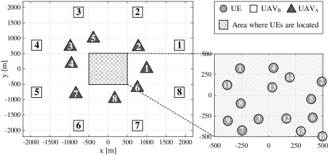
Figure 4: Test scenario for numerical evaluation.

Fig. 4 shows the test scenario used for performance evaluation and comparison in this section, which consists of 8 UAV_A (${N_{A}}=8$), 8 UAV_B (${N_{B}}=8$) and 15 UEs ($M=15$). The origin of Cartesian coordinates is set at the center of the test scenario. UAV_B are uniformly deployed on the circle of radius 2 km centered at the origin, and the distance between each UAV_B and its corresponding BS is 1 km. The horizontal coordinates of the 8 UAV_A’s HPs are set to ${\bf{q}}_{1}^{\circ}\!=\!{\left[{1000,0}\right]^{T}}$, ${\bf{q}}_{2}^{\circ}\!=\!{\left[{785,715}\right]^{T}}$, ${\bf{q}}_{3}^{\circ}\!=\!{\left[{-980,724}\right]^{T}}$, ${\bf{q}}_{4}^{\circ}\!=\!{\left[{-951,164}\right]^{T}}$, ${\bf{q}}_{5}^{\circ}\!=\!{\left[{-382,990}\right]^{T}}$, ${\bf{q}}_{6}^{\circ}\!=\!{\left[{758,-624}\right]^{T}}$, ${\bf{q}}_{7}^{\circ}\!=\!{\left[{-836,-820}\right]^{T}}$ and ${\bf{q}}_{8}^{\circ}\!=\!{\left[{172,-977}\right]^{T}}$. UEs are randomly located within a square with center at the coordinate origin and side length of 1 km. When assigning $N_{A}^{U}$ UAV_A to each UE, we select the subset of UAV_A with the minimum horizontal dilution of precision (HDOP) [14]. The same criterion is also used for the selection of the three UAV_B responsible for sensing each UAV_A’s state.

The key simulation parameters used in this section are summarized as follows: All UAVs in the proposed system, including UAV_A and UAV_B, hover at the same altitude ${h_{v}}\!=\!50$ m and have the same transmit power ${P_{t}}\!=\!30$ dBm; The noise power at terrestrial BSs is ${N_{0}}\!=\!-107$ dBm; The number of UAV_A serving each UE is $N_{A}^{U}=3$; The variances of inter-UAV and UAV_A-UE distance measurements are $\sigma_{d}^{2}=1$ ${{\rm m^{2}}}$ and $\sigma_{r}^{2}=1$ ${{\rm m^{2}}}$, respectively; UEs have the same requirement on the MSE of positioning services, i.e., $MS{E_{Req,m}}={10^{2}}$ ${{\rm m^{2}}}$ ($\forall m\in{\cal M}$). The covariance matrices of velocity and acceleration measurements are set to ${{\bf{R}}_{\bf{v}}}=\left({{{0.5}^{2}}}\right)\cdot{{\bf{I}}_{2}}$ and ${{\bf{R}}_{\bf{a}}}=\left({{{0.1}^{2}}}\right)\cdot{{\bf{I}}_{2}}$, respectively; The length of each time slot is $\Delta t=1$ s; The time constant of lag of each UAV_A in responding commanded acceleration is $\rho=10$ ms; The continuous-time acceleration process noise intensity in $x$- and $y$-directions are $\varsigma_{x}^{2}={0.5^{2}}$ ${{{m^{2}}}\mathord{\left/{\vphantom{{{m^{2}}}{{s^{3}}}}}\right.\kern-1.2pt}{{s^{3}}}}$ and $\varsigma_{y}^{2}={0.5^{2}}$ ${{{m^{2}}}\mathord{\left/{\vphantom{{{m^{2}}}{{s^{3}}}}}\right.\kern-1.2pt}{{s^{3}}}}$, respectively; The feedback gain matrix ${{\bf{K}}_{j}}$ for UAV control is generated based on the standard linear quadratic regulator (LQR) control; The scaling factor and success rate in the proposed co-design scheme are set to $\lambda=0.8$ and $P_{Req}^{\left(c\right)}=0.95$, respectively.

V-A The Importance of Co-Design in UAV-Enabled Positioning

In this subsection, we successively apply two UAV-enabled positioning systems, namely the conventional system without considering state sensing and control as well as the proposed co-design system, in the test scenario shown in Fig. 4. The proposed system operates according to the scheme described in Section IV, while the dynamics model of the conventional system is obtained by removing the term ${{\bf{B}}_{j}}{{\bf{u}}_{j,t}}$ from equation (11). The running time of both systems is 60 time slots (1 min), and the corresponding simulation results are shown in Fig. 5 and Fig. 6. For the simplicity of data presentation, this subsection only presents the simulation results corresponding to a part of UAV_A and UEs, which will not reduce the generality of the analysis results.

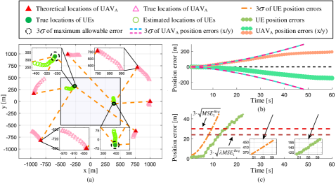
Figure 5: Test results of the system without UAV state sensing: Variations of (a) system status, (b) UAV control error (${\rm UAV_{A}}$ 7) and (c) UE positioning performance (UE 1).

Fig. 5(a) and Fig. 6(a) show the variations of the two systems’ statuses over time, including the variations of UAV_A’s true locations and UEs’ location estimates. The location estimate of each UE is obtained through the ILS method introduced in Section II.C, and the estimation is performed once in each time slot. It can be seen that UAV_A in the conventional system deviate significantly from their HPs. According to Fig. 5(b), these deviations reach hundreds of meters in both $x$- and $y$-directions after 40 s, almost threatening the system safety. In terms of QoS, as can be seen from Fig. 5(c), the theoretical MSE of the conventional system’s positioning services exceeds the ${10^{2}}$ ${m^{2}}$ required by UEs only 10 s after the experiment starts. About 5 s later, the position estimation error of ILS also exceeds the tolerable limit. At the end of the experiment, the theoretical MSE and position error of the conventional system have reached the astonishing values of ${156.7^{2}}$ ${m^{2}}$ and $164.2$ m, respectively. These phenomena indicate that sensing and control functionalities are indispensable for the implementation of UAV-enabled positioning.

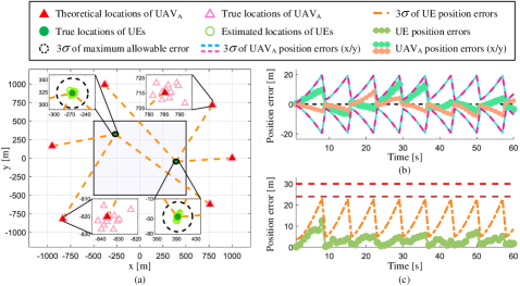
Figure 6: Test results of the proposed system using the co-design scheme: Variations of (a) system status, (b) UAV control error (${\rm UAV_{A}}$ 7) and (c) UE positioning performance (UE 1).

As shown in Fig. 6(a), during the experiment, UAV_A in the proposed system always stay in the vicinity of their HPs, and the position estimation error of each UE is also kept within an acceptable range. According to Fig. 6(b), the proposed system maintains the deviations between UAV_A’s true location and its HP in both $x$- and $y$-directions within the range of $-20.00\sim 20.00$ m. The variation of UAV control error in Fig. 6(b) can be interpreted as follows: When the position uncertainty of the UAV_A is relatively small, such as $1\!\sim\!7$ s in this experiment, UAV_A is controlled in OL mode to reduce resource consumption, resulting in an increase in UAV control error. If the UAV position uncertainty approaches the limit defined by inequality (46), the proposed system allocates wireless resources for state sensing to the UAV_A so that it can be controlled in CL mode. Therefore, the UAV control errors in our system fluctuate dynamically with time. Moreover, as can be seen from Fig. 6(c), the theoretical MSE of our system’s positioning services exhibits a variation similar to the variance of the UAV control error. This phenomenon is reasonable because, according to equation (35), the position uncertainty of UAV_A is one of the main factors affecting the performance of UE positioning. It is noteworthy that although the quality of positioning services fluctuates with time, the proposed system can always meet UEs’ requirements. During the experiment, the maximum theoretical MSE and position estimation error are ${7.717^{2}}$ ${m^{2}}$ and $12.44$ m, respectively. The above results demonstrate the feasibility and validity of our system and scheme.

The simulation results in this subsection reflect the importance of state sensing and control for UAV-enabled positioning, as well as the validity of the proposed co-design system. In addition, it can be seen that in both UAV control and UE position estimation, the measured error rarely exceeds three times the theoretical root-mean-square error (RMSE), which demonstrates the correctness of the performance analysis in Section III.

V-B The Superiority of Co-Design over the Continuous Scheme

In this subsection, we test and compare the performance of our scheme introduced in Section IV and the “continuous scheme” commonly used in existing systems to illustrate the superiority of SCC co-design. In the continuous scheme, the state sensing for each UAV_A is performed in each time slot, i.e., ${\varphi_{j,t}}=1$ ($\forall j\in{{\cal N}_{A}}$, $\forall t$). The blocklength in the continuous scheme is determined by the same strategy shown in equation (52). Fig. 7 and Fig. 8 show the numerical results obtained in this experiment.

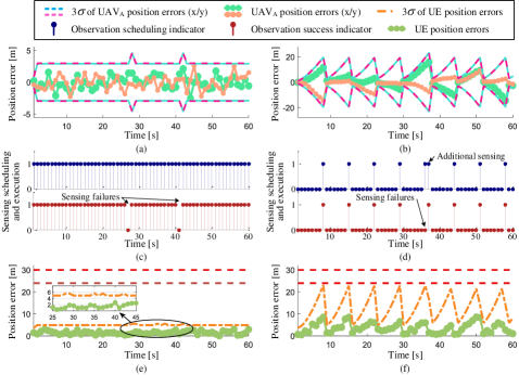
Figure 7: Performance comparison between the continuous and proposed schemes: UAV control error (${\rm UAV_{A}}$ 7) of the (a) continuous and (b) proposed schemes; Sensing scheduling and execution status (${\rm UAV_{A}}$ 7) of the (c) continuous and (d) proposed schemes; UE positioning performance (UE 1) of the (e) continuous and (f) proposed schemes

As can be seen from Fig. 7(a) and (b), the UAV control error of the continuous scheme is basically maintained within the range of $-2.973\sim 2.973$ m, while that of the proposed system is mostly between $-19.33$ m and $19.33$ m. Please note that in the 28 s and 42 s of the operation of the continuous scheme, the envelope of UAV control error expands significantly and reaches $\pm 4.607$ m. According to the sensing scheduling and execution results shown in Fig. 7(c), the major cause of these phenomena is the unexpected OL control due to the failures of sensing data transmission in 27 s and 41 s. As shown in Fig. 7(b) and (d), a similar phenomenon also occurs in the 37 s of the operation of the proposed scheme. Fortunately, the proposed scheme performs additional state sensing in the 37 s, avoiding the further increase in the variance of UAV control error. This result indicates the proposed scheme’s adaptability to transmission failures. Although it seems that the continuous scheme has much smaller UAV control errors than the proposed scheme, the data in Fig. 7(e) and (f) show that such high control accuracy is completely unnecessary for positioning services. According to Fig. 7(e), during the experiment, the maximum theoretical MSE and position estimation error of the continuous scheme’s positioning services are ${1.847^{2}}$ ${m^{2}}$ and $3.023$ m, which are far below the UEs’ tolerable limits. In terms of the proposed system (Fig. 7(f)), its maximum theoretical MSE and position error are ${7.717^{2}}$ ${m^{2}}$ and $8.537$ m, which are much larger than those of the continuous scheme but still meet the UEs’ requirements.

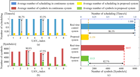
Figure 8: Performance comparison between the continuous and proposed schemes: Number of (a) scheduling and (b) symbols corresponding to each ${\rm UAV_{A}}$ in two schemes; (c) average number of scheduling and symbols among all ${\rm UAV_{A}}$ in two schemes.

Since both of the schemes tested in this subsection could satisfy UEs’ QoS demands, we turn to compare their resource consumption. The average number of scheduling (times/s) and the average number of symbols (symbols/s) used for data transmission are chosen as the metrics for evaluating the resource efficiency of each scheme. Fig. 8 shows the comparison of the resource consumption of the two schemes. As can be seen from Fig. 8(a), compared with the continuous scheme, the proposed scheme significantly reduces the average number of scheduling for each UAV_A. The reduction in the number of scheduling is between $83.3\%$ and $86.7\%$. Moreover, according to Fig. 8(b), the proposed scheme also greatly reduces the number of symbols required for the state sensing of each UAV_A, and the reduction is within the range of $67.5\%\sim 90.9\%$. Fig. 8(c) shows the resource consumption of the two schemes from an overall system perspective. For the overall system, the proposed scheme reduces the number of scheduling and symbols for positioning services by $86.1\%$ and $82.7\%$, respectively.

Based on the above numerical results, the superiority of the proposed SCC co-design scheme over the commonly used continuous scheme can be summarized as follows: The capabilities of state sensing and prediction in the proposed scheme enable the system to schedule and allocate resources flexibly according to the system status, thereby improving the resource efficiency of positioning services while ensuring that QoS meets UEs’ requirements.

V-C The Superiority of Co-Design over the Periodic Scheme

The simulation results presented in the previous two subsections (especially Fig. 6(b) and Fig. 7(d)) may give the illusion that the state sensing in the proposed scheme is performed periodically. Therefore, in this subsection, we compare our SCC co-design scheme with the periodic scheme to illustrate the differences between the two schemes as well as the superiority of the proposed scheme. In the periodic scheme, the state sensing for each UAV_A is performed periodically at a constant time interval, regardless of whether the sensing data is successfully transmitted. For the parameter setting mentioned at the beginning of this section, this time interval is set to 7 time slots (i.e., 7 s). We set up two test situations for the comparison of the two schemes, namely the low-success-rate situation and the intermittent-link-blocking situation. In each situation, the running time of both schemes is 120 time slots (2 min).

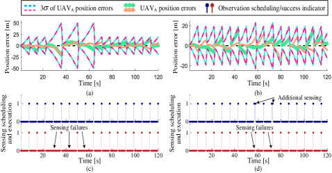
Figure 9: Performance comparison between the periodic and proposed schemes under low-success-rate condition: UAV control error (${\rm UAV_{A}}$ 7) of the (a) periodic and (b) proposed schemes; Sensing scheduling and execution status (${\rm UAV_{A}}$ 7) of the (c) periodic and (d) proposed schemes.

In the low-success-rate situation, the success rate of state sensing ($P_{Req}^{\left(c\right)}$) is reduced from 0.95 to 0.70, so as to simulate frequent transmission failures due to limited wireless resources and fading channels. The values of other parameters are the same as those mentioned at the beginning of this section. Fig. 9 and Fig. 10 show the performance of the two schemes in this test situation. As can be seen from Fig. 9(c), in the 29 s, 43 s and 57 s of the operation of the periodic scheme, the state sensing for the UAV_A is scheduled but not successfully executed. According to Fig. 9(a), the envelope of UAV control error continues to expand after these moments until state sensing is scheduled and executed successfully in the next “sensing occasion”. During the experiment, the size of the envelope of UAV control error in the periodic scheme reaches a maximum of $\pm 50.05$ m. For the proposed scheme, the deviation between UAV_A’s true location and its HP is basically maintained within the range of $-19.33\sim 19.33$ m, as shown in Fig. 9(b). Although sensing failures also occur in the proposed scheme (57 s and 72 s in Fig. 9(d)) and lead to temporary expansions of the envelope of UAV control error, these trends are quickly reversed by performing additional state sensing in the next time slots (58 s and 73 s). The differences in sensing scheduling between the two schemes also affect the quality of their positioning services. As shown in Fig. 10(a), during the experiment, the theoretical MSE of the periodic scheme exceeds the tolerable limit several times, resulting in “service failures”. On the contrary, as can be seen from Fig. 10(b), the performance of the proposed scheme’s positioning services always meets UEs’ requirements. According to the sensing scheduling and execution results shown in Fig. 10(c) and (d), the main reason for these phenomena is that the proposed scheme has the ability to perform additional state sensing according to the system status, while the periodic scheme does not. Therefore, in the low-success-rate situation, the service of the proposed SCC co-design scheme is much more reliable than that of the periodic scheme.

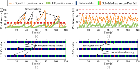
Figure 10: Performance comparison between the periodic and proposed schemes under low-success-rate condition: UE positioning performance (UE 1) of the (a) periodic and (b) proposed schemes; Sensing scheduling and execution status (${\rm UAV_{A}}$ 4, 6 and 7 that serve UE 1) of the (c) periodic and (d) proposed schemes.

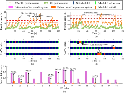
Figure 11: Performance comparison between the periodic and proposed schemes under intermittent-link-blocking condition: UE positioning performance (UE 1) of the (a) periodic and (b) proposed schemes; Sensing scheduling and execution status (${\rm UAV_{A}}$ 4, 6 and 7 that serve UE 1) of the (c) periodic and (d) proposed schemes; (e) Service failure rate corresponding to each UE in two schemes

The term “intermittent-link-blocking” refers to a situation where one or more UAV_A are unable to perform state sensing within a short period of time due to equipment failure or other reasons. In this experiment, we assume that the sensing links for UAV_A 4, 6 and 7 are blocked in the time periods of $63\sim 72$ s, $98\sim 103$ s and $20\sim 24$ s, respectively. Fig. 11 shows the test results of the two schemes obtained in this situation. As can be seen from Fig. 11 (a) and (b), service failures occur during the operation of both schemes. However, it is worth noting that the number and duration of service failures in the proposed scheme are much smaller than those in the periodic scheme. Moreover, during the experiment, the maximum theoretical MSE of the periodic and proposed schemes is ${18.47^{2}}$ ${m^{2}}$ and ${12.01^{2}}$ ${m^{2}}$, respectively. Thus, compared with the periodic scheme, the proposed scheme also significantly reduces the impact of link blocking on the quality of positioning services. In Fig. 11(e), the service failure rate of each UE in the experiment is calculated. It can be seen clearly that the proposed scheme greatly reduces the service failure rate of each of the 15 UEs in the system, and the reduction ranges from $76.2\%$ to $96.3\%$. The data in Fig. 11(c) and (d) illustrate that the proposed scheme’s ability to perform additional state sensing is also the major cause of these phenomena.

From the above experimental results and analysis, it can be concluded that the capabilities of state sensing and prediction enable our proposed SCC co-design scheme to achieve much better service reliability than the periodic scheme in harsh situations.

V-D Key Factors Affecting System Performance

The validity of the proposed system and its superiority over the benchmark schemes have been demonstrated in the previous subsections. Then, in this subsection, we conduct two experiments to analyze the key factors affecting the performance of the proposed system and their influence on positioning services. Specifically, we consider three factors, namely the tolerable limit of the theoretical MSE of positioning services ($MS{E_{Req,m}}$), the scaling factor ($\lambda$) and success rate ($P_{Req}^{\left(c\right)}$) in the proposed scheme. The system performance is evaluated by the following three metrics: service failure rate, average number of scheduling and average number of symbols. In order to make the experimental results statistically significant, the running time of our system in each experiment is set to $1\times{10^{6}}$ time slots (about 11.6 days).

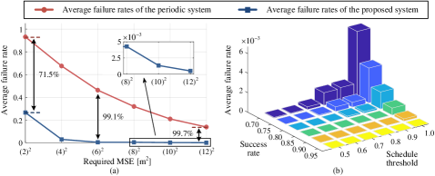
Figure 12: Variations of service failure rate with (a) Required RMSE, (b) success rate and schedule threshold.

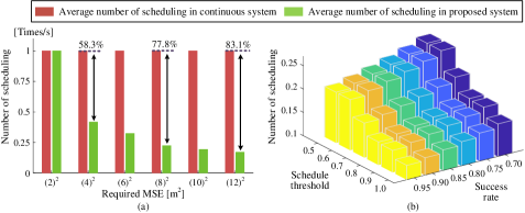
Figure 13: Variations of average number of scheduling with (a) Required RMSE, (b) success rate and schedule threshold.

In the first experiment, we analyze the influence of UEs’ tolerable limit ($MS{E_{Req,m}}$) on system performance. During the simulation, the value of $MS{E_{Req,m}}$ increases from ${2^{2}}$ ${m^{2}}$ to ${12^{2}}$ ${m^{2}}$, while the values of other parameters are set according to the parameter setting mentioned at the beginning of this section. Fig. 12(a), Fig. 13(a) and Fig. 14(a) show the variations of the three performance metrics with the value of $MS{E_{Req,m}}$. As can be seen from Fig. 12(a), the service failure rate of the proposed system decreases with the increase of $MS{E_{Req,m}}$. Moreover, the advantage of the proposed system over the periodic system in service reliability becomes more significant as $MS{E_{Req,m}}$ increases. When $MS{E_{Req,m}}={2^{2}}$ ${m^{2}}$, the service failure rate of the proposed system is $71.5\%$ lower than that of the periodic system, and this ratio increases to $99.7\%$ after the value of $MS{E_{Req,m}}$ becomes ${12^{2}}$ ${m^{2}}$. In terms of the average number of scheduling and symbols, according to Fig. 13(a) and Fig. 14(a), these two performance metrics of the proposed system also decrease with the increase of $MS{E_{Req,m}}$. Since the resource consumption of the continuous system remains basically unchanged during the experiment, the reduction of the resource consumption in the proposed system highlights its advantage in resource efficiency. For example, when $MS{E_{Req,m}}={2^{2}}$ ${m^{2}}$, the proposed system has the same resource consumption as the continuous system. However, when the value of $MS{E_{Req,m}}$ increases to ${12^{2}}$ ${m^{2}}$, the average number of scheduling and average number of symbols in the proposed system are $83.1\%$ and $82.6\%$ less than those in the continuous system. The main reason for these phenomena is that the proposed system has the ability to adjust the frequency of state sensing flexibly according to UEs’ requirements, while the continuous system does not. The above experimental results indicate that the proposed system has more significant advantages in service reliability and resource efficiency when UEs have relatively loose requirements on position accuracy.

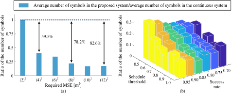
Figure 14: Variations of average number of symbols with (a) Required RMSE, (b) success rate and schedule threshold.

Then, another experiment is conducted to analyze the influence of parameters $\lambda$ and $P_{Req}^{\left(c\right)}$ on system performance. During the simulation, the value of $P_{Req}^{\left(c\right)}$ increases from 0.70 to 0.95, while $\lambda$ varies from 0.5 to 1.0. The values of other parameters are the same as those described at the beginning of this section. Fig. 12(b), Fig. 13(b) and Fig. 14(b) show the variations of the proposed system’s performance metrics with the values of $\lambda$ and $P_{Req}^{\left(c\right)}$. According to Fig. 12(b), the service failure rate of the proposed system decreases rapidly with the increase of $P_{Req}^{\left(c\right)}$ and the decrease of $\lambda$. When $\lambda\leq 0.8$ and $P_{Req}^{\left(c\right)}\geq 0.80$, the service failure rate is lower than $1.435\times{10^{-4}}$, which is negligible for some applications without requirements for high reliability. As can be seen from Fig. 13(b), the average number of scheduling decreases as $\lambda$ and $P_{Req}^{\left(c\right)}$ increase. The average number of scheduling obtained at $\left[{\lambda,P_{Req}^{\left(c\right)}}\right]=\left[{1.0,0.95}\right]$ is 0.1307 times/s, which is only $49.6\%$ of the 0.2633 times/s obtained at $\left[{0.5,0.7}\right]$. However, it is noteworthy that large values of $\lambda$ may lead to high service failure rates. Thus, in practice, the value of $\lambda$ should be selected carefully according to system’s requirements for service reliability and resource efficiency. As shown in Fig. 14(b), the average number of symbols in the proposed system fluctuates with the values of $\lambda$ and $P_{Req}^{\left(c\right)}$, and its variation is quite complicated. The reason for this phenomenon can be intuitively interpreted as follows: Although reducing $P_{Req}^{\left(c\right)}$ could reduce the number of symbols used in each sensing occasion, it also increases the sensing failure rate (Fig. 12(b)), resulting in more additional state sensing (Fig. 13(b)). Therefore, there is no monotonic relationship between the average number of symbols and the value of $P_{Req}^{\left(c\right)}$. The influence of $\lambda$ can be interpreted in the same way. The non-monotonic relationships shown in Fig. 14(b) indicate that it is possible to find a set of $\lambda$ and $P_{Req}^{\left(c\right)}$ that provide the best balance of QoS and resource efficiency, which remains an open question in this article and will be studied in our future work.

VI Conclusion

In this article, a novel UAV-enabled positioning system is proposed based on the concept of SCC co-design to provide positioning services that meet UEs’ requirements and have high resource efficiency. Different from previous research, we considered the cooperation of sensing, communication and control functionalities in the system design, and studied many issues that have often been overlooked. Specifically, we first established the structure and mathematical models of our system. Then, the UAV stability in open-loop and closed-loop operation modes as well as the theoretical MSE of positioning services in the presence of UAV control errors was derived. It was found that the scheduling of UAV state sensing and blocklength for the transmission of sensing data are two main factors affecting the quality and resource consumption of positioning services. Thus, we further studied the problem of joint sensing scheduling and blocklength allocation, and developed a novel scheme to solve this mixed-integer nonlinear optimization problem efficiently. Numerical results demonstrated that compared with two benchmark systems, the proposed system improves the service reliability and resource efficiency by more than 76.2$\%$ or 82.7$\%$, respectively. We hope this article could lead to a new paradigm for the design of UAV-enabled positioning systems and bring inspiration for the application of SCC co-design concept in UAV systems.

Appendix A Model of TWR Technique

In the proposed system, the TWR technique is selected to measure inter-UAV distances and the distances between UEs and UAV_A. In this appendix, we take the inter-UAV distance measurement between the $j$-th UAV_A and $i$-th UAV_B as an example to establish the mathematical model of TWR. As shown in Fig. 14, the TWR begins with a request message sent by the $i$-th UAV_B at local time $t_{i}^{s}$. After receiving the request message, the $j$-th UAV_A sends back a response message after a fixed response delay ${\tau_{D}}$ [37], which will be detected by the UAV_B at its local time $\hat{t}_{i}^{r}$. The time interval between the transmission of the request message and the reception of the response message measured by UAV_B’s local clock can be expressed as [15]

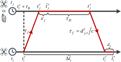
Figure 15: Time diagram of TWR.

$$\Delta{\hat{t}_{i}}=\hat{t}_{i}^{r}-t_{i}^{s}=2{\tau_{f}}\left({1+{\delta_{i}}}\right)+\left({{\tau_{D}}+{\varepsilon_{j}}}\right)\cdot\frac{{\left({1+{\delta_{i}}}\right)}}{{\left({1+{\delta_{j}}}\right)}}+{\varepsilon_{i}},$$ (53)

where ${\tau_{f}}$ is the time of flight (ToF); ${\delta_{j}}$ and ${\delta_{i}}$ denote the clock drifts of the $j$-th UAV_A and $i$-th UAV_B relative to the reference clock, respectively; ${\varepsilon_{j}}$ and ${\varepsilon_{i}}$ are measurement errors caused by UAVs’ internal noise.

Then, the estimate of ToF can be written as

$$\begin{split}{{\hat{\tau}}_{f}}=\frac{1}{2}\left({\Delta{{\hat{t}}_{i}}-{\tau_{D}}}\right)&={\tau_{f}}\left({1+{\delta_{i}}}\right)+\frac{{{\tau_{D}}\left({{\delta_{i}}-{\delta_{j}}}\right)+{\varepsilon_{j}}\left({1+{\delta_{i}}}\right)}}{{2\left({1+{\delta_{j}}}\right)}}+\frac{{{\varepsilon_{i}}}}{2}\\ &\approx{\tau_{f}}+\frac{{{\tau_{D}}\left({{\delta_{i}}-{\delta_{j}}}\right)}}{2}+\frac{{{\varepsilon_{j}}}}{2}+\frac{{{\varepsilon_{i}}}}{2}\approx{\tau_{f}}+\frac{{{\tau_{D}}\left({{\delta_{i}}-{\delta_{j}}}\right)}}{2}.\end{split}$$ (54)

Please note that in the above equation, the expression of ${\hat{\tau}_{f}}$ has been approximated based on the fact that ${\delta_{j}}\ll 1$ (${\delta_{i}}\ll 1$) and ${\varepsilon_{j}}\ll{\tau_{D}}\left({{\delta_{i}}-{\delta_{j}}}\right)$ (${\varepsilon_{i}}\ll{\tau_{D}}\left({{\delta_{i}}-{\delta_{j}}}\right)$) [15].

Thus, the distance measurement obtained by the TWR technique is given by

$$\hat{d}_{j,t}^{i}=c\cdot{\hat{\tau}_{f}}=c\cdot{\tau_{f}}+\frac{{c\cdot{\tau_{D}}\left({{\delta_{i}}-{\delta_{j}}}\!\right)}}{2}=d_{j,t}^{i}+n_{d,j,t}^{i},$$ (55)

where $n_{d,j,t}^{i}={{c\cdot{\tau_{D}}\left({{\delta_{i}}-{\delta_{j}}}\right)}\mathord{\left/{\vphantom{{c\cdot{\tau_{D}}\left({{\delta_{i}}-{\delta_{j}}}\right)}2}}\right.\kern-1.2pt}2}$ denotes the distance measurement error caused by clock drifts. Without loss of generality, $n_{d,j,t}^{i}$ could be modeled as zero-mean Gaussian noise, that is, $n_{d,j,t}^{i}\sim\left({0,\sigma_{d}^{2}}\right)$ [15, 38].

Appendix B UAV Dynamics Model

Since this article is just a preliminary attempt to introduce the SCC co-design concept into UAV-enabled positioning, we simply use the following third-order linear model to describe the dynamics of the $j$-th UAV_A:

$$\Delta\dot{q}_{j}^{\left(x\right)}=v_{j}^{\left(x\right)},\qquad\qquad\qquad\quad\;\Delta\dot{q}_{j}^{\left(y\right)}=v_{j}^{\left(y\right)},\qquad\qquad$$ (56)

$$\dot{v}_{j}^{\left(x\right)}=a_{j}^{\left(x\right)},\qquad\qquad\qquad\qquad\,\dot{v}_{j}^{\left(y\right)}=a_{j}^{\left(y\right)},\qquad\qquad\;\;\,$$ (57)

$$\quad\;\,\dot{a}_{j}^{\left(x\right)}=-\frac{1}{\rho}a_{j}^{\left(x\right)}+\frac{1}{\rho}u_{j}^{\left(x\right)},\qquad\quad\;\dot{a}_{j}^{\left(x\right)}=-\frac{1}{\rho}a_{j}^{\left(x\right)}+\frac{1}{\rho}u_{j}^{\left(x\right)},\quad\,$$ (58)

The discrete-time version of the above model in the $x$-direction can be written as

$$\Delta q_{j,t+1}^{\left(x\right)}\!=\!\Delta q_{j,t}^{\left(x\right)}\!+\!\Delta t\cdot v_{j,t}^{\left(x\right)}\!+\!\left({{\rho^{2}}{e^{-{{\Delta t}\mathord{\left/{\vphantom{{\Delta t}\rho}}\right.\kern-1.2pt}\rho}}}\!+\!\rho\Delta t\!-\!{\rho^{2}}}\right)\!a_{j,t}^{\left(x\right)}\!+\!\left[{{\rho^{2}}\!\left(\!{-{e^{-{{\Delta t}\mathord{\left/{\vphantom{{\Delta t}\rho}}\right.\kern-1.2pt}\rho}}}\!+\!1}\!\right)+\Delta t\left({-\rho\!+\!\Delta t}\right)}\right]u_{j,t}^{\left(x\right)},$$ (59)

$$v_{j,t+1}^{\left(x\right)}=v_{j,t}^{\left(x\right)}+\rho\left({1-{e^{-{{\Delta t}\mathord{\left/{\vphantom{{\Delta t}\rho}}\right.\kern-1.2pt}\rho}}}}\right)a_{j,t}^{\left(x\right)}+\left[{\Delta t+\rho\left({{e^{-{{\Delta t}\mathord{\left/{\vphantom{{\Delta t}\rho}}\right.\kern-1.2pt}\rho}}}-1}\right)}\right]u_{j,t}^{\left(x\right)},$$ (60)

$$a_{j,t+1}^{\left(x\right)}={e^{-{{\Delta t}\mathord{\left/{\vphantom{{\Delta t}\rho}}\right.\kern-1.2pt}\rho}}}a_{j,t}^{\left(x\right)}+\left({1-{e^{-{{\Delta t}\mathord{\left/{\vphantom{{\Delta t}\rho}}\right.\kern-1.2pt}\rho}}}}\right)u_{j,t}^{\left(x\right)},$$ (61)

The discrete-time dynamics model in the $y$-direction can be expressed in the same way and will not be repeated here. Then, the expression for matrix ${{\bf{A}}_{j}}$ in equation (11) is given by

$${{\bf{A}}_{j}}=\left[{\begin{array}[]{*{20}{c}}{{{\bf{A}}_{j,1}}}&{{{\bf{A}}_{j,2}}}\end{array}}\right],$$ (62)

where

$${{\bf{A}}_{j,1}}={\left[{\begin{array}[]{*{20}{c}}1&0&0&0&0&0\\ 0&1&0&0&0&0\\ {\Delta t}&0&1&0&0&0\\ 0&{\Delta t}&0&1&0&0\end{array}}\right]^{T}},$$ (63)

$${{\bf{A}}_{j,2}}=\left[{\begin{array}[]{*{20}{c}}{{\rho^{2}}{e^{-{{\Delta t}\mathord{\left/{\vphantom{{\Delta t}\rho}}\right.\kern-1.2pt}\rho}}}+\rho\Delta t-{\rho^{2}}}&0\\ 0&{{\rho^{2}}{e^{-{{\Delta t}\mathord{\left/{\vphantom{{\Delta t}\rho}}\right.\kern-1.2pt}\rho}}}+\rho\Delta t-{\rho^{2}}}\\ {\rho\left({1-{e^{-{{\Delta t}\mathord{\left/{\vphantom{{\Delta t}\rho}}\right.\kern-1.2pt}\rho}}}}\right)}&0\\ 0&{\rho\left({1-{e^{-{{\Delta t}\mathord{\left/{\vphantom{{\Delta t}\rho}}\right.\kern-1.2pt}\rho}}}}\right)}\\ {{e^{-{{\Delta t}\mathord{\left/{\vphantom{{\Delta t}\rho}}\right.\kern-1.2pt}\rho}}}}&0\\ 0&{{e^{-{{\Delta t}\mathord{\left/{\vphantom{{\Delta t}\rho}}\right.\kern-1.2pt}\rho}}}}\end{array}}\right].$$ (64)

Similarly, the expression for matrix ${{\bf{B}}_{j}}$ can be written as

$${{\bf{B}}_{j}}=\left[{\begin{array}[]{*{20}{c}}\begin{array}[]{l}{\rho^{2}}\left({-{e^{-{{\Delta t}\mathord{\left/{\vphantom{{\Delta t}\rho}}\right.\kern-1.2pt}\rho}}}+1}\right)\\ \quad+\Delta t\left({-\rho+\Delta t}\right)\end{array}&0\\ 0&\begin{array}[]{l}{\rho^{2}}\left({-{e^{-{{\Delta t}\mathord{\left/{\vphantom{{\Delta t}\rho}}\right.\kern-1.2pt}\rho}}}+1}\right)\\ \quad+\Delta t\left({-\rho+\Delta t}\right)\end{array}\\ {\Delta t+\rho\left({{e^{-{{\Delta t}\mathord{\left/{\vphantom{{\Delta t}\rho}}\right.\kern-1.2pt}\rho}}}-1}\!\right)}&0\\ 0&{\Delta t+\rho\left({{e^{-{{\Delta t}\mathord{\left/{\vphantom{{\Delta t}\rho}}\right.\kern-1.2pt}\rho}}}-1}\right)}\\ {1-{e^{-{{\Delta t}\mathord{\left/{\vphantom{{\Delta t}\rho}}\right.\kern-1.2pt}\rho}}}}&0\\ 0&{1-{e^{-{{\Delta t}\mathord{\left/{\vphantom{{\Delta t}\rho}}\right.\kern-1.2pt}\rho}}}}\end{array}}\right].$$ (65)

For the covariance matrix (${{\bf{Q}}_{\bf{w}}}$) of process noise (${{\bf{w}}_{j,t}}$), it can be expressed as [39]

$${{\bf{Q}}_{\bf{w}}}=E\left\{{{{\bf{w}}_{j,t}}{\bf{w}}_{j,t}^{T}}\right\}=\left[{\begin{array}[]{*{20}{c}}{{{\bf{Q}}_{{\bf{w}},1}}}&{{\bf{0}}{}_{4\times 2}}\\ {{\bf{0}}{}_{2\times 4}}&{{{\bf{Q}}_{{\bf{w}},2}}}\end{array}}\right],$$ (66)

where

$${{\bf{Q}}_{{\bf{w}},1}}=\left[{\begin{array}[]{*{20}{c}}{{\raise 3.01385pt\hbox{${\Delta{t^{3}}\varsigma_{x}^{2}}$}\mathord{\left/{\vphantom{{\Delta{t^{3}}\varsigma_{x}^{2}}3}}\right.\kern-1.2pt}\lower 3.01385pt\hbox{$3$}}}&0&{{\raise 3.01385pt\hbox{${\Delta{t^{2}}\varsigma_{x}^{2}}$}\mathord{\left/{\vphantom{{\Delta{t^{2}}\varsigma_{x}^{2}}2}}\right.\kern-1.2pt}\lower 3.01385pt\hbox{$2$}}}&0\\ 0&{{\raise 3.01385pt\hbox{${\Delta{t^{3}}\varsigma_{y}^{2}}$}\mathord{\left/{\vphantom{{\Delta{t^{3}}\varsigma_{y}^{2}}3}}\right.\kern-1.2pt}\lower 3.01385pt\hbox{$3$}}}&0&{{\raise 3.01385pt\hbox{${\Delta{t^{2}}\varsigma_{y}^{2}}$}\mathord{\left/{\vphantom{{\Delta{t^{2}}\varsigma_{y}^{2}}2}}\right.\kern-1.2pt}\lower 3.01385pt\hbox{$2$}}}\\ {{\raise 3.01385pt\hbox{${\Delta{t^{2}}\varsigma_{x}^{2}}$}\mathord{\left/{\vphantom{{\Delta{t^{2}}\varsigma_{x}^{2}}2}}\right.\kern-1.2pt}\lower 3.01385pt\hbox{$2$}}}&0&{\Delta t\cdot\varsigma_{x}^{2}}&0\\ 0&{{\raise 3.01385pt\hbox{${\Delta{t^{2}}\varsigma_{y}^{2}}$}\mathord{\left/{\vphantom{{\Delta{t^{2}}\varsigma_{y}^{2}}2}}\right.\kern-1.2pt}\lower 3.01385pt\hbox{$2$}}}&0&{\Delta t\cdot\varsigma_{y}^{2}}\end{array}}\right],$$ (67)

$${{\bf{Q}}_{{\bf{w}},2}}={\rm diag}(\varsigma_{x}^{2},\varsigma_{y}^{2});$$ (68)

Parameters $\varsigma_{x}^{2}$ and $\varsigma_{y}^{2}$ represent the continuous-time acceleration process noise intensity in $x$- and $y$-directions, respectively.

Appendix C Relationship between Blocklength and Transmission Success Rate

In this article, the A2G link between the $i$-th UAV_B and its corresponding BS is modeled as a Rayleigh fading channel, whose channel power gain is represented by ${\left|{{h_{i,t}}}\right|^{2}}$. Denote the transmit power of UAV_B and the noise power at BS as ${P_{t}}$ and ${N_{0}}$, then the SNR of the $i$-th UAV_B’s signal at BS can be expressed as

$${\gamma_{i,t}}=\left({{{{P_{t}}}\mathord{\left/{\vphantom{{{P_{t}}}{{N_{0}}}}}\right.\kern-1.2pt}{{N_{0}}}}}\right)\cdot{\left|{{h_{i,t}}}\right|^{2}},$$ (69)

According to [40], if the number of symbols used to transmit the sensing data corresponding to the $j$-th UAV_A and $i$-th UAV_B in time slot $t$ is $\theta_{j,t}^{i}$, the success rate of data transmission can be calculated as

$${P^{\left(s\right)}}\!\left({\theta_{j,t}^{i},{\gamma_{i,t}}}\right)=1-Q\left({f\left({\theta_{j,t}^{i},{\gamma_{i,t}}}\right)}\right),$$ (70)

where $Q\left(x\right)={\left({2\pi}\right)^{{{-1}\mathord{\left/{\vphantom{{-1}2}}\right.\kern-1.2pt}2}}}\int_{x}^{\infty}{{e^{{{-{z^{2}}}\mathord{\left/{\vphantom{{-{z^{2}}}2}}\right.\kern-1.2pt}2}}}dz}$, and

$$f\left({\theta_{j,t}^{i},{\gamma_{i,t}}}\right)=\ln\left(2\right)\sqrt{\frac{{\theta_{j,t}^{i}}}{{{V_{i,t}}}}}\cdot\left[{{{\log}_{2}}\left({1+{\gamma_{i,t}}}\right)-\frac{D}{{\theta_{j,t}^{i}}}}\right];$$ (71)

$D$ is the size of sensing data (bits) and ${V_{i,t}}=1-{\left({1+{\gamma_{i,t}}}\right)^{-2}}$.

Conversely, for a given success rate $P_{j,t}^{i,\left(s\right)}$ ($P_{j,t}^{i,\left(s\right)}\geq 0.5$), the minimum number of symbols required for data transmission is given by

$$\begin{split}\theta\!\left(\!{P_{j,t}^{i,\left(s\right)},{\gamma_{i,t}}}\!\right)&=2D\!\cdot\!\left\{\!{\frac{{{V_{i,t}}}}{D}\!\cdot\!{{\left(\!{\frac{{{Q^{-1}}\!\left(\!{1\!-\!P_{j,t}^{i,\left(s\right)}}\!\right)}}{{\ln\left(2\right)}}}\!\right)}^{2}}\!+\!2{{\log}_{2}}\!\left(\!{1\!+\!{\gamma_{i,t}}}\!\right)\!-\!\left[\!{\frac{{V_{i,t}^{2}}}{{{D^{2}}}}\!\cdot\!{{\left(\!{\frac{{{Q^{-1}}\!\left(\!{1\!-\!P_{j,t}^{i,\left(s\right)}}\!\right)}}{{\ln\left(2\right)}}}\right)}^{4}}}\!\right.}\!\right.\\ &{\left.{{{\left.{\left.{+4{{\log}_{2}}\!\left(\!1\right.\!+\!{\gamma_{i,t}}}\!\right)\!\left(\!{\frac{{{V_{i,t}}}}{D}}\!\right)\!{{\left(\!{\frac{{{Q^{-1}}\left(\!{1\!-\!P_{j,t}^{i,\left(s\right)}}\!\right)}}{{\ln\left(2\right)}}}\!\right)}^{2}}}\right]}^{\frac{1}{2}}}}\!\right\}^{-1}},\qquad\qquad\;P_{j,t}^{i,\left(s\right)}\geq 0.5.\end{split}$$ (72)

Appendix D Proof of Proposition 1

According to equations (43), (44) and (47), $\sigma_{\Delta{\bf{q}},m}^{2}\cdot{{\bf{I}}_{{N_{A}^{U}}}}-{{\bf{\bar{D}}}_{\Delta{\bf{q}},m,t+1}}\left({{{\bm{\varphi}}_{t}},{{\bm{\theta}}_{t}}}\right)$ is a diagonal matrix. Thus, we have

$$\begin{split}&{\mathop{\rm tr}\nolimits}\left({{\bf{S}}\left({{{\bf{p}}_{m}}}\right)\left({\sigma_{\Delta{\bf{q}},m}^{2}\cdot{{\bf{I}}_{{N_{A}^{U}}}}-{{{\bf{\bar{D}}}}_{\Delta{\bf{q}}.m,t+1}}\left({{{\bm{\varphi}}_{t}},{{\bm{\theta}}_{t}}}\!\right)}\right){\bf{S}}{{\left({{{\bf{p}}_{m}}}\right)}^{T}}}\right)\\ &\qquad\qquad\qquad\qquad=\sum\limits_{l=1}^{2}{{{\bf{s}}_{l}}\left({{{\bf{p}}_{m}}}\right)\left({\sigma_{\Delta{\bf{q}},m}^{2}\cdot{{\bf{I}}_{{N_{A}^{U}}}}-{{{\bf{\bar{D}}}}_{\Delta{\bf{q}},m,t+1}}\left({{{\bm{\varphi}}_{t}},{{\bm{\theta}}_{t}}}\right)}\right){{\bf{s}}_{l}}{{\left({{{\bf{p}}_{m}}}\right)}\!^{T}}},\end{split}$$ (73)

where ${{\bf{s}}_{l}}\left({{{\bf{p}}_{m}}}\right)$ represents the $l$-th row vector of matrix ${\bf{S}}\left({{{\bf{p}}_{m}}}\right)$. Moreover, if condition (46) is satisfied, the elements in diagonal matrix $\sigma_{\Delta{\bf{q}},m}^{2}\cdot{{\bf{I}}_{{N_{A}^{U}}}}-{{\bf{\bar{D}}}_{\Delta{\bf{q}},m,t+1}}\left({{{\bm{\varphi}}_{t}},{{\bm{\theta}}_{t}}}\right)$ are all non-negative, which means that it is a positive semi-definite (PSD) matrix. According to the definition of PSD matrices, we have

$${{\bf{s}}_{l}}\left({{{\bf{p}}_{m}}}\right)\left({\sigma_{\Delta{\bf{q}},m}^{2}\cdot{{\bf{I}}_{{N_{A}^{U}}}}-{{{\bf{\bar{D}}}}_{\Delta{\bf{q}}.m,t+1}}\left({{{\bm{\varphi}}_{t}},{{\bm{\theta}}_{t}}}\right)}\right){{\bf{s}}_{l}}{\left({{{\bf{p}}_{m}}}\right)^{T}}\geq 0.$$ (74)

Then, the following inequality holds:

$${\mathop{\rm tr}\nolimits}\left({{\bf{S}}\left({{{\bf{p}}_{m}}}\right)\left({\sigma_{\Delta{\bf{q}},m}^{2}\cdot{{\bf{I}}_{{N_{A}^{U}}}}-{{{\bf{\bar{D}}}}_{\Delta{\bf{q}}.m,t+1}}\left({{{\bm{\varphi}}_{t}},{{\bm{\theta}}_{t}}}\right)}\right){\bf{S}}{{\left({{{\bf{p}}_{m}}}\right)}^{T}}}\right)\geq 0.$$ (75)

Finally, we have

$$\begin{split}{\mathop{\rm tr}\nolimits}&\left({{\bf{S}}\left({{{\bf{p}}_{m}}}\right){{{\bf{\bar{D}}}}_{\Delta{\bf{q}}.m,t+1}}\left({{{\bm{\varphi}}_{t}},{{\bm{\theta}}_{t}}}\right){\bf{S}}{{\left({{{\bf{p}}_{m}}}\right)}^{T}}}\right)\leq{\mathop{\rm tr}\nolimits}\left({{\bf{S}}\left({{{\bf{p}}_{m}}}\right)\left({\sigma_{\Delta{\bf{q}},m}^{2}\cdot{{\bf{I}}_{{N_{A}^{U}}}}}\right){\bf{S}}{{\left({{{\bf{p}}_{m}}}\right)}^{T}}}\right)\\ &\qquad\qquad\qquad\qquad=\sigma_{\Delta{\bf{q}},m}^{2}\cdot{\mathop{\rm tr}\nolimits}\left({{\bf{S}}\left({{{\bf{p}}_{m}}}\right){\bf{S}}{{\left({{{\bf{p}}_{m}}}\right)}^{T}}}\right)=\sigma_{\Delta{\bf{q}},m}^{2}\cdot{\mathop{\rm tr}\nolimits}\left({{\bf{P}}\left({{{\bf{p}}_{m}}}\right)}\right)=Th{r_{m}}.\end{split}$$ (76)

This completes the proof of Proposition 1.

References

• [1] H. Huang, G. Gartner, J. M. Krisp, M. Raubal, and N. Van de Weghe, “Location based services: Ongoing evolution and research agenda,” Journal of Location Based Services, vol. 12, no. 2, pp. 63–93, 2018.
• [2] R. Keating, M. Säily, J. Hulkkonen, and J. Karjalainen, “Overview of positioning in 5G new radio,” in 2019 16th International Symposium on Wireless Communication Systems (ISWCS), 2019, pp. 320–324.
• [3] S. Dang, O. Amin, B. Shihada, and M.-S. Alouini, “What should 6G be?” Nature Electronics, vol. 3, no. 1, pp. 20–29, 2020.
• [4] B. Xu, Q. Jia, and L.-T. Hsu, “Vector tracking loop-based GNSS NLOS detection and correction: Algorithm design and performance analysis,” IEEE Transactions on Instrumentation and Measurement, vol. 69, no. 7, pp. 4604–4619, 2020.
• [5] D. Lu, S. Jiang, B. Cai, W. Shangguan, K. Liu, and J. Luan, “Quantitative analysis of GNSS performance under railway obstruction environment,” in 2018 IEEE/ION Position, Location and Navigation Symposium (PLANS), 2018, pp. 1074–1080.
• [6] P. A. Zandbergen, “Accuracy of iphone locations: A comparison of assisted GPS, WiFi and cellular positioning,” Transactions in GIS, vol. 13, no. s1, pp. 5–25, 2009.
• [7] K. Shamaei and Z. M. Kassas, “LTE receiver design and multipath analysis for navigation in urban environments,” NAVIGATION, vol. 65, no. 4, pp. 655–675, 2018.
• [8] Q. Liu, R. Liu, Z. Wang, and Y. Zhang, “Simulation and analysis of device positioning in 5G ultra-dense network,” in 2019 15th International Wireless Communications $\&$ Mobile Computing Conference (IWCMC), 2019, pp. 1529–1533.
• [9] Y. Zeng, Q. Wu, and R. Zhang, “Accessing from the sky: A tutorial on UAV communications for 5G and beyond,” Proceedings of the IEEE, vol. 107, no. 12, pp. 2327–2375, 2019.
• [10] Z. Wang, L. Duan, and R. Zhang, “Adaptive deployment for UAV-aided communication networks,” IEEE Transactions on Wireless Communications, vol. 18, no. 9, pp. 4531–4543, 2019.
• [11] S. Zeng, H. Zhang, B. Di, and L. Song, “Trajectory optimization and resource allocation for OFDMA UAV relay networks,” IEEE Transactions on Wireless Communications, pp. 1–1, 2021.
• [12] M. Mozaffari, W. Saad, M. Bennis, and M. Debbah, “Mobile unmanned aerial vehicles (UAVs) for energy-efficient internet of things communications,” IEEE Transactions on Wireless Communications, vol. 16, no. 11, pp. 7574–7589, 2017.
• [13] G. Han, J. Jiang, C. Zhang, T. Q. Duong, M. Guizani, and G. K. Karagiannidis, “A survey on mobile anchor node assisted localization in wireless sensor networks,” IEEE Communications Surveys $\&$ Tutorials, vol. 18, no. 3, pp. 2220–2243, 2016.
• [14] Z. Wang, R. Liu, Q. Liu, J. S. Thompson, and M. Kadoch, “Energy-efficient data collection and device positioning in UAV-assisted IoT,” IEEE Internet of Things Journal, vol. 7, no. 2, pp. 1122–1139, 2020.
• [15] Z. Wang, R. Liu, Q. Liu, L. Han, J. S. Thompson, Y. Lin, and W. Mu, “Toward reliable UAV-enabled positioning in mountainous environments: System design and preliminary results,” IEEE Transactions on Reliability, pp. 1–29, 2021.
• [16] S. Zhang, R. Pöhlmann, E. Staudinger, and A. Dammann, “Assembling a swarm navigation system: Communication, localization, sensing and control,” in 2021 IEEE 18th Annual Consumer Communications $\&$ Networking Conference (CCNC), 2021, pp. 1–9.
• [17] G. Zhao, M. A. Imran, Z. Pang, Z. Chen, and L. Li, “Toward real-time control in future wireless networks: Communication-control co-design,” IEEE Communications Magazine, vol. 57, no. 2, pp. 138–144, 2019.
• [18] C. De Lima et al., “Convergent communication, sensing and localization in 6G systems: An overview of technologies, opportunities and challenges,” IEEE Access, vol. 9, pp. 26 902–26 925, 2021.
• [19] M. Z. Chowdhury, M. Shahjalal, S. Ahmed, and Y. M. Jang, “6G wireless communication systems: Applications, requirements, technologies, challenges, and research directions,” IEEE Open Journal of the Communications Society, vol. 1, pp. 957–975, 2020.
• [20] Z. Xiao and Y. Zeng, “An overview on integrated localization and communication towards 6G,” arXiv preprint arXiv:2006.01535, 2020.
• [21] J. Park, S. Samarakoon, H. Shiri, M. K. Abdel-Aziz, T. Nishio, A. Elgabli, and M. Bennis, “Extreme URLLC: Vision, challenges, and key enablers,” arXiv preprint arXiv:2001.09683, 2020.
• [22] J. Zhao, F. Gao, G. Ding, T. Zhang, W. Jia, and A. Nallanathan, “Integrating communications and control for UAV systems: Opportunities and challenges,” IEEE Access, vol. 6, pp. 67 519–67 527, 2018.
• [23] H. Sallouha, M. M. Azari, A. Chiumento, and S. Pollin, “Aerial anchors positioning for reliable RSS-based outdoor localization in urban environments,” IEEE Wireless Communications Letters, vol. 7, no. 3, pp. 376–379, 2018.
• [24] H. Sallouha, M. M. Azari, and S. Pollin, “Energy-constrained UAV trajectory design for ground node localization,” in 2018 IEEE Global Communications Conference (GLOBECOM), 2018, pp. 1–7.
• [25] Z. Wang, R. Liu, Q. Liu, L. Han, and J. S. Thompson, “Feasibility study of UAV-assisted anti-jamming positioning,” IEEE Transactions on Vehicular Technology, pp. 1–1, 2021.
• [26] Q. Liu, R. Liu, Z. Wang, and J. S. Thompson, “UAV swarm-enabled localization in isolated region: A rigidity-constrained deployment perspective,” IEEE Wireless Communications Letters, pp. 1–1, 2021.
• [27] Y. Liu, Y. Wang, J. Wang, and Y. Shen, “Distributed 3D relative localization of UAVs,” IEEE Transactions on Vehicular Technology, vol. 69, no. 10, pp. 11 756–11 770, 2020.
• [28] F. Wang and H. Li, “Joint power allocation for radar and communication co-existence,” IEEE Signal Processing Letters, vol. 26, no. 11, pp. 1608–1612, 2019.
• [29] F. Liu, C. Masouros, A. P. Petropulu, H. Griffiths, and L. Hanzo, “Joint radar and communication design: Applications, state-of-the-art, and the road ahead,” IEEE Transactions on Communications, vol. 68, no. 6, pp. 3834–3862, 2020.
• [30] W. Yuan, F. Liu, C. Masouros, J. Yuan, D. W. K. Ng, and N. González-Prelcic, “Bayesian predictive beamforming for vehicular networks: A low-overhead joint radar-communication approach,” IEEE Transactions on Wireless Communications, vol. 20, no. 3, pp. 1442–1456, 2021.
• [31] J. Mei, K. Zheng, L. Zhao, L. Lei, and X. Wang, “Joint radio resource allocation and control for vehicle platooning in LTE-V2V network,” IEEE Transactions on Vehicular Technology, vol. 67, no. 12, pp. 12 218–12 230, 2018.
• [32] A. González, N. Franchi, and G. Fettweis, “Control loop aware LTE-V2X semi-persistent scheduling for string stable CACC,” in 2019 IEEE 30th Annual International Symposium on Personal, Indoor and Mobile Radio Communications (PIMRC), 2019, pp. 1–7.
• [33] M. Eisen, M. M. Rashid, K. Gatsis, D. Cavalcanti, N. Himayat, and A. Ribeiro, “Control aware radio resource allocation in low latency wireless control systems,” IEEE Internet of Things Journal, vol. 6, no. 5, pp. 7878–7890, 2019.
• [34] Y. Wu, Q. Yang, H. Li, K. S. Kwak, and V. C. M. Leung, “Control-aware energy-efficient transmissions for wireless control systems with short packets,” IEEE Internet of Things Journal, pp. 1–1, 2021.
• [35] K. C. Ho, X. Lu, and L. Kovavisaruch, “Source localization using TDOA and FDOA measurements in the presence of receiver location errors: Analysis and solution,” IEEE Transactions on Signal Processing, vol. 55, no. 2, pp. 684–696, 2007.
• [36] W. H. FOY, “Position-location solutions by Taylor-series estimation,” IEEE Transactions on Aerospace and Electronic Systems, vol. AES-12, no. 2, pp. 187–194, 1976.
• [37] S. Frattasi and F. Della Rosa, Mobile positioning and tracking: from conventional to cooperative techniques.   John Wiley $\&$ Sons, 2017.
• [38] E. Akyol, K. Viswanatha, and K. Rose, “On conditions for linearity of optimal estimation,” IEEE Transactions on Information Theory, vol. 58, no. 6, pp. 3497–3508, 2012.
• [39] S. Ragothaman, M. Maaref, and Z. M. Kassas, “Multipath-optimal UAV trajectory planning for urban UAV navigation with cellular signals,” in 2019 IEEE 90th Vehicular Technology Conference (VTC2019-Fall), 2019, pp. 1–6.
• [40] C. Pan, H. Ren, Y. Deng, M. Elkashlan, and A. Nallanathan, “Joint blocklength and location optimization for URLLC-enabled UAV relay systems,” IEEE Communications Letters, vol. 23, no. 3, pp. 498–501, 2019.