SDSS J154751.94+025550 with double-peaked broad H$\beta$ but single-peaked broad H$\alpha$: a candidate for central binary black hole system?

Abstract

In this manuscript, an interesting blue Active Galactic Nuclei (AGN) SDSS J154751.94+025550 (=SDSS J1547) is reported with very different line profiles of broad Balmer emission lines: double-peaked broad H$\beta$ but single-peaked broad H$\alpha$. SDSS J1547 is the first AGN with detailed discussions on very different line profiles of the broad Balmer emission lines, besides the simply mentioned different broad lines in the candidate for a binary black hole (BBH) system in SDSS J0159+0105. The very different line profiles of the broad Balmer emission lines can be well explained by different physical conditions to two central BLRs in a central BBH system in SDSS J1547. Furthermore, the long-term light curve from CSS can be well described by a sinusoidal function with a periodicity about 2159days, providing further evidence to support the expected central BBH system in SDSS J1547. Therefore, it is interesting to treat different line profiles of broad Balmer emission lines as intrinsic indicators of central BBH systems in broad line AGN. Under assumptions of BBH systems, 0.125% of broad line AGN can be expected to have very different line profiles of broad Balmer emission lines. Future study on more broad line AGN with very different line profiles of broad Balmer emission lines could provide further clues on the different line profiles of broad Balmer emission lines as indicator of BBH systems.

1 Introduction

Broad emission lines from central broad line regions (BLRs) are fundamental characteristics of broad line Active Galactic Nuclei (AGN) (Sulentic et al., 2000; Gaskell, 2009; Kollatschny & Zetzl, 2013; Vietri et al., 2020). Due to limitations of modern observational techniques, central BLRs with distances of tens to hundreds of light-days (Kaspi et al., 2000; Bentz et al., 2013) to central black holes (BHs) cannot be directly spatial resolved. Detailed structures of central BLRs are determined through broad line emission features, especially long-term variabilities of broad emission lines. And then, different geometric structures of central BLRs have been reported, such as disk-like BLRs especially determined through double-peaked broad emission lines (Chen & Halpern, 1989; Eracleous et al., 2005; Storchi-Bergmann et al., 2003; Zhang, 2013b; Storchi-Bergmann et al., 2017), as structures determined through modeling the continuum variability and response in emission-line profile changes as a function of time (Grier et al., 2013, 2017; De Rosa et al., 2018; Brotherton et al., 2020).

Among the broad emission lines in broad line AGN, broad H$\alpha$ and broad H$\beta$ are the two strongest optical recombination emission lines, such as the detailed emission line properties in composite spectrum of AGN and quasars as discussed in Brotherton et al. (2001); Vanden Berk et al. (2001). Not similar as the commonly considered different emission regions between high-ionization broad lines and low-ionization broad lines (Braibant et al., 2016), broad Balmer lines are well accepted to come from the totally same emission regions. Therefore, totally similar line profiles of broad Balmer emission lines are expected due to totally similar dynamical structures. And as the discussed results in large samples of broad line AGN and quasars in Greene & Ho (2005), similar line profiles of broad Balmer lines have been well reported, such as the reported strong linear line width correlation between broad Balmer lines in SDSS quasars.

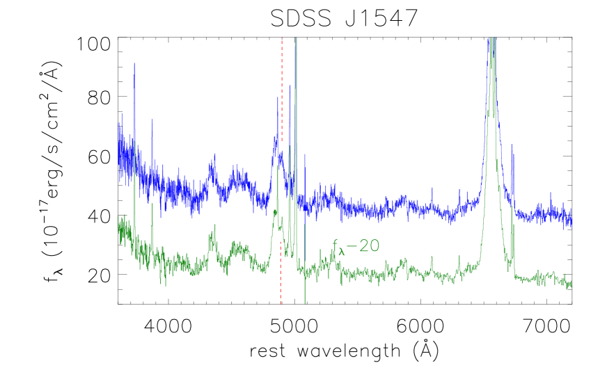
Figure 1: SDSS spectra of SDSS J1547. Solid blue line shows the spectrum observed in MJD=52027, solid dark green line shows the spectrum observed in MJD=52045 with $f_{\lambda}$ minus 20. Vertical dashed red line marks the second peak position in the broad H$\beta$.

However, if there were two central distinct BLRs with large distance enough for the broad Balmer emission lines, the observed broad Balmer emission lines should include two broad components from the two BLRs. Once there were different dust obscurations on the two BLRs or different physical local conditions (different ionization parameters, different electron densities, etc.) of the two BLRs, different line profiles of the observed broad Balmer emission lines could be expected due to the different circumstances around the two BLRs. The case of different obscurations is not easy to be imagined, unless the two BLRs have space distance very large enough. Whereas, the case of different physical local conditions can be well and commonly expected in AGN, especially in the well-known supermassive binary black hole (BBH) systems in AGN. BBH systems have been thought to be inevitable outcomes of the merger-driven galactic evolutions (Begelman et al., 1980; Taniguchi & Wada, 1996; Volonteri et al., 2003; Di Matteo et al., 2005; Cuadra et al., 2009; Khan et al., 2012; Pfister et al., 2017; Sayeb et al., 2021). And candidates for BBH systems have been reported in dozens of active galaxies through different techniques, especially based on properties of either spectroscopic properties or long-term variability properties combining with spatially resolved images, such as the reported candidates for BBH systems in Zhou et al. (2004); Rodriguez et al. (2009); Shen & Loeb (2010); Graham et al. (2015a, b); Liu et al. (2016); De Rosa et al. (2019); Kollatschny et al. (2020); Liao et al. (2021). In a BBH system, each BH accreting system has a surrounding BLRs with dependent physical local parameters of ionization parameters, electron temperature, electron density, etc.. Therefore, different physical local conditions of the two BLRs could be common in BBH systems, and it is interesting to detect different line profiles of broad Balmer emission lines in broad line AGN harbouring BBH systems.

In the manuscript, we report the robust and confirmed different line profiles of broad Balmer lines in the broad line AGN SDSS J1547: the double-peaked broad H$\beta$ and the broad H$\gamma$ but the single-peaked broad H$\alpha$, which could provide further clues on a central probable BBH system. In Section 2, the main spectroscopic results are shown. In Section 3, accretion disk origin of the broad Balmer emission lines are mainly discussed, providing evidence to rule out the accretion disk origin to explain the different line profiles of broad Balmer emission lines of SDSS J1547. In Section 4, BBH model is mainly discussed in SDSS J1547, confirmed by the detected optical quasi-periodic oscillations in the long-term variabilities of SDSS J1547. In Section 5, we simply discuss how many AGN similar as SDSS J1547  can be found in SDSS (Sloan Digital Sky Survey). In Section 6, the main conclusions are given. And in the manuscript, we have adopted the cosmological parameters of $H_{0}=70{\rm km\cdot s}^{-1}{\rm Mpc}^{-1}$, $\Omega_{\Lambda}=0.7$ and $\Omega_{\rm m}=0.3$.

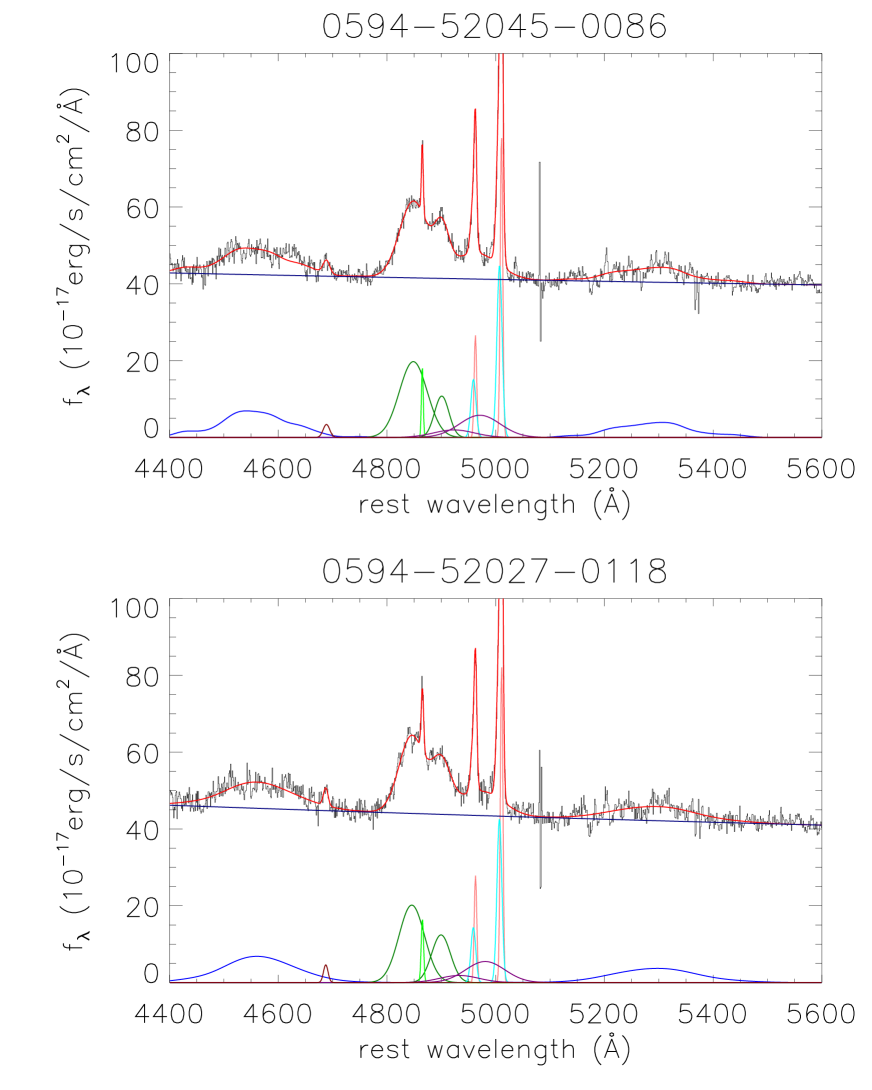
Figure 2: Best descriptions to the emission lines around H$\beta$ in MJD=52045 (top panel) and in MJD=52027 (bottom panel). In each panel, solid black line and solid red line show the line spectrum and the determined best descriptions, respectively. Solid dark blue line shows the determined AGN continuum emissions, solid blue line shows the determined optical Fe ii emissions, solid dark green lines show the determined two broad Gaussian components in the broad H$\beta$, solid green line shows the determined narrow H$\beta$, solid pink and cyan lines show the determined core and broad [O iii] components, solid purple lines show the determined extremely extended broad [O iii] components, solid dark red line shows the determined broad He ii line.

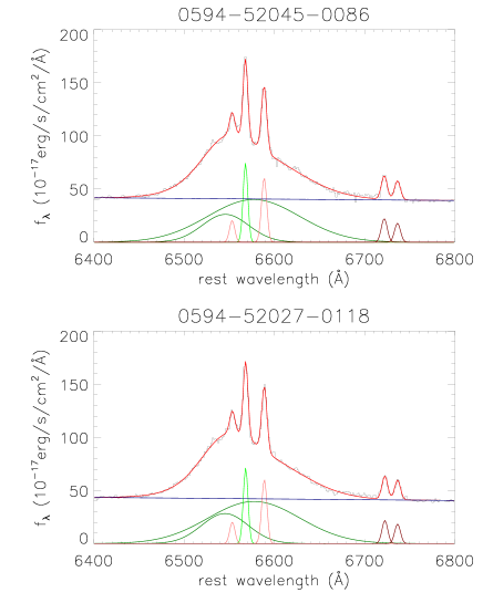
Figure 3: Best descriptions to the emission lines around H$\alpha$ in MJD=52045 (top panel) and in MJD=52027 (bottom panel). In each panel, solid black line and solid red line show the line spectrum and the determined best descriptions, respectively. Solid dark blue line shows the determined AGN continuum emissions, solid dark green lines show the determined two broad Gaussian components in the broad H$\alpha$, solid green line shows the determined narrow H$\alpha$, solid pink lines show the determined [N ii] doublet, solid dark red lines shows the determined [S ii] doublet.

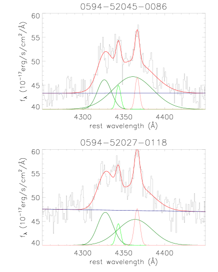
Figure 4: Best descriptions to the emission lines around H$\gamma$ in MJD=52045 (top panel) and in MJD=52027 (bottom panel). In each panel, solid black line and solid red line show the line spectrum and the determined best descriptions, respectively. Solid dark blue line shows the determined AGN continuum emissions, solid dark green lines show the determined two broad Gaussian components in the broad H$\gamma$, solid green line shows the determined narrow H$\gamma$, solid pink lines show the determined [O iii]$\lambda 4364$Å.

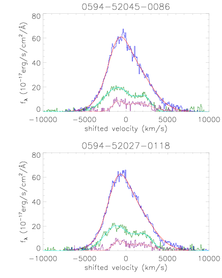
Figure 5: Line profiles of the broad H$\alpha$, the broad H$\beta$ and the broad H$\gamma$ in velocity space in MJD=52045 (top panel) and in MJD=52027 (bottom panel), after subtractions of both the narrow emission line components and the continuum emissions component. In each panel, solid line in blue, dark green and purple shows the line profile of the broad H$\alpha$, of the broad H$\beta$ and of the broad H$\gamma$, respectively, solid line in red, cyan and pink shows the corresponding best-fitting results to the broad H$\alpha$, the broad H$\beta$ and the broad H$\gamma$ by the two broad Gaussian components shown as solid dark green lines in Figure 2, in Figure 3 and in Figure 4, respectively.

2 Spectroscopic Properties in SDSS J1547

SDSS J1547 at redshift of 0.09768 has been observed twice in one month in SDSS (Gunn et al., 2006; Ahumada et al., 2020). The SDSS spectra (information of PLATE-MJD-FIBERID: 0594-52027-0118 and 0594-52045-0086) are collected from SDSS DR16 (Data Release 16) and shown in Figure 1. Based on the spectroscopic features, SDSS J1547 is a broad line AGN with apparently broad Balmer emissions. And through the shown spectra, there is an interesting point that there is an additional peak (marked by vertical dashed red line in Figure 1) in the broad H$\beta$ but not in the broad H$\alpha$. The double-peaked broad H$\beta$ but single-peaked broad H$\alpha$ can be confirmed in the repeated spectra of SDSS J1547, indicating the strange features could be not due to observational mistakes. Meanwhile, SDSS J1547 (also named as MS 1545.3+0305) has also been observed by the Clay Telescope and shown in Figure 1 in Ho & Kim (2009) with the apparent double-peaked features in the broad H$\beta$.

In order to well confirm the different line profiles of the broad H$\beta$ and the broad H$\alpha$, the following model functions are accepted to describe the emission lines around H$\beta$ and around H$\alpha$. Similar as what we have done in the more recent paper Zhang (2021), for the emission lines around H$\beta$ with rest wavelength range from 4400Å to 5600Å, there are two broad Gaussian functions applied to describe the broad H$\beta$, three narrow Gaussian functions applied to describe the narrow H$\beta$ and the core [O iii] components, two another Gaussian functions applied to describe the broad [O iii] components, two another additional broad Gaussian functions applied to describe the extremely extended broad [O iii] components (which will be discussed in detail in the follows), one broad Gaussian function applied to describe weak He ii line, one power law function $P_{\lambda}=\alpha\times(\lambda/5100\text{\AA})^{\beta}$ applied to describe AGN continuum emissions, and the broadened and scaled Fe ii templates discussed in Kovacevic et al. (2010) applied to describe the strong optical Fe ii lines. Based on the widely applied Levenberg-Marquardt least-squares minimization technique, the best-fitting results to the emission lines around H$\beta$ can be well determined, and shown in Figure 2, with the determined $\chi^{2}=SSR/Dof$ (where $SSR$ and $Dof$ as summed squared residuals and degree of freedom) about 1.41 and 1.06 for the emission lines observed in MJD=52045 and in MJD=52027, respectively. The determined line parameters of central wavelength, second moment and line flux of each emission component are listed in Table 1.

The emission lines around H$\alpha$ with rest wavelength range from 6400Å  to 6800Å  can be well described by the following model functions. There are two broad Gaussian functions applied to describe the broad H$\alpha$, five narrow Gaussian functions applied to describe the narrow H$\alpha$, the [N ii] doublet and the [S ii] doublet. Then, through the Levenberg-Marquardt least-squares minimization technique, the best descriptions to the emission lines around H$\alpha$ can be well determined and shown in Figure 3, with the determined $\chi^{2}=SSR/Dof$ about 1.81 and 0.99 for the emission lines observed in MJD=52045 and in MJD=52027, respectively. The corresponding line parameters are also listed in Table 1.

Before proceeding further, we show further discussions on the extremely extended broad [O iii] components around 4975Å  shown as solid purple lines in Figure 2. If the broad components were not the [O iii] emission components, but from broad H$\beta$ emissions, it could be expect that there should be similar broad components in the broad H$\alpha$ around 6720Å. However, such expected broad emission components in broad H$\alpha$ cannot be found. Therefore, the broad components around 4975Å  are accepted as the extremely extended broad [O iii] components in SDSS J1547, not part of the broad H$\beta$ emissions.

Meanwhile, properties of broad H$\gamma$ are also considered. The best-fitting results to the emission lines around H$\gamma$ are shown in Figure 4, based on the similar model functions: two broad Gaussian functions for the broad H$\gamma$, one narrow Gaussian function for the narrow H$\gamma$ and one narrow Gaussian function for the [O iii]$\lambda 4364$Å. The determined line parameters are also listed in Table 1. Then, in order to clearly show the compared line profiles between the broad Balmer emission lines, the line profiles are shown in velocity space in Figure 5. It is obvious that there are two peaks around -1103${\rm km/s}$ and 2180${\rm km/s}$ in the broad H$\beta$ and also in the broad H$\gamma$, but only one apparent peak around -750${\rm km/s}$ in the broad H$\alpha$.

Whether the different line profiles of broad Balmer emission lines could be due to effects of different optical depths of broad Balmer emission lines? The effects of different optical depths have been well discussed in Korista & Goad (2004); Bentz et al. (2010) and in more recent discussed results in Netzer (2020), leading to expected longer distance of emission regions and smaller line width of broad H$\alpha$ than those of broad H$\beta$ and broad H$\gamma$, because broad H$\alpha$ has the largest optical depth among the broad Balmer emission lines. Therefore, the line widths of broad H$\alpha$, broad H$\beta$ and broad H$\gamma$ are firstly checked. Based on the shown line profiles $p_{\lambda}$ of the broad Balmer emission lines in Figure 5 and the definition of second moment $\sigma_{l}$ of emission lines in Peterson et al. (2004),

$$\begin{split}&\lambda_{0}~{}=~{}\frac{\int~{}\lambda~{}p_{\lambda}d\lambda}{\int~{}p_{\lambda}d\lambda}\\ &\sigma_{l}^{2}~{}=~{}\frac{\int~{}\lambda^{2}~{}p_{\lambda}d\lambda}{\int~{}p_{\lambda}d\lambda}~{}-~{}\lambda_{0}^{2}\end{split}$$ (1)

, the line widths are measured as 47.8Å  (2184${\rm km/s}$), 31.9Å  (1968${\rm km/s}$) and 26.3Å  (1817${\rm km/s}$) of broad H$\alpha$, broad H$\beta$ and broad H$\gamma$, respectively. It is clear that broad H$\alpha$ has line width (second moment) larger than broad H$\beta$ and broad H$\gamma$, not consistent with the expected results after considerations of effects of different optical depths of broad Balmer emission lines. Meanwhile, the FWHMs (full widths at half maximum) of the broad Balmer emission lines can be measured as 101.7Å  (4648${\rm km/s}$), 90.9Å  (5608${\rm km/s}$) and 67.8Å  (4685${\rm km/s}$) of broad H$\alpha$, broad H$\beta$ and broad H$\gamma$, respectively. Even considering the FWHMs as the line width, although the broad H$\alpha$ is broader than the broad H$\beta$, the broad H$\beta$ quite narrower than the broad H$\gamma$, not consistent with the expected results after considerations of effects of different optical depths of broad Balmer emission lines. Therefore, effects of different optical depths of broad Balmer emission lines can not be preferred to explain the different profiles of broad Balmer emission lines, and there are no further discussions on the effects in the manuscript.

Based on the results shown in Figure 2, Figure 3 and Figure 4 and in Figure 5, the very different line profiles can be well detected between the broad H$\alpha$ and the broad H$\beta$. Furthermore, based on the measured line parameters, the flux ratio of total broad H$\alpha$ to total broad H$\beta$ is about 4.08, and the flux ratio of narrow H$\alpha$ to narrow H$\beta$ is about 5.7. The larger flux ratio in narrow Balmer lines than in broad Balmer lines indicates that the flux ratio of broad Balmer lines is not due to commonly accepted obscurations, otherwise there should be larger flux ratio of broad H$\alpha$ to broad H$\beta$ than the ratio of narrow H$\alpha$ to narrow H$\beta$. Furthermore, in spite of the lower spectral quality around H$\gamma$, the larger flux ratio 14 of the narrow H$\alpha$ to the narrow H$\gamma$ than the flux ratio 12 of the broad H$\alpha$ to the broad H$\gamma$, providing further evidence that the commonly accepted obscurations should be not preferred in SDSS J1547. Therefore, accretion disk origin and different intrinsic physical conditions are mainly considered to explain the different line profiles between the broad Balmer lines in SDSS J1547.

Table 1: Line parameters of emission lines of SDSS J1547

parameters in MJD=52045
Line	$\lambda_{0}$	$\sigma$	flux
H$\alpha_{B1}$	6545.7$\pm$0.9	25.8$\pm$1.1	1683$\pm$151
H$\alpha_{B2}$	6576.9$\pm$1.2	50.9$\pm$0.6	5118$\pm$159
H$\beta_{B1}$	4848.4$\pm$0.9	25.6$\pm$0.9	1267$\pm$46
H$\beta_{B2}$	4900.7$\pm$0.9	13.2$\pm$1.1	357$\pm$44
H$\gamma_{B1}$	4326.1$\pm$1.1	8.6$\pm$1.6	132$\pm$42
H$\gamma_{B2}$	4361.1$\pm$3.9	24.2$\pm$3.9	415$\pm$72
H$\alpha_{N}$	6567.9$\pm$0.1	2.6$\pm$0.1	487$\pm$15
H$\beta_{N}$	4864.9$\pm$0.1	1.6$\pm$0.1	77$\pm$7
H$\gamma_{N}$	4343.4$\pm$0.4	2.8$\pm$0.8	36$\pm$12
[O iii]$\lambda 4364$Å	4366.4$\pm$0.4	2.7$\pm$0.5	45$\pm$9
[O iii]c	5010.5$\pm$0.1	2.3$\pm$0.1	463$\pm$39
[O iii]B	5006.9$\pm$0.3	4.8$\pm$0.2	536$\pm$43
[O iii]E	4970.8$\pm$3.3	37.5$\pm$3.3	542$\pm$41
[N ii]	6588.6$\pm$0.1	2.9$\pm$0.1	444$\pm$14
[S ii]$\lambda 6716$Å	6721.6$\pm$0.1	3.3$\pm$0.1	181$\pm$7
[S ii]$\lambda 6731$Å	6736.3$\pm$0.2	3.3$\pm$0.1	145$\pm$6
parameters in MJD=52027
H$\alpha_{B1}$	6545.2$\pm$1.1	25.8$\pm$1.2	1830$\pm$194
H$\alpha_{B2}$	6577.4$\pm$1.6	50.7$\pm$0.8	5049$\pm$206
H$\beta_{B1}$	4845.6$\pm$1.6	23.5$\pm$1.3	1188$\pm$74
H$\beta_{B2}$	4899.4$\pm$1.8	17.3$\pm$1.6	537$\pm$78
H$\gamma_{B1}$	4327.4$\pm$1.6	9.5$\pm$1.8	163$\pm$49
H$\gamma_{B2}$	4363.7$\pm$4.8	20.9$\pm$5.1	282$\pm$66
H$\alpha_{N}$	6568.1$\pm$0.1	2.6$\pm$0.1	470$\pm$18
H$\beta_{N}$	4865.1$\pm$0.2	2.2$\pm$0.2	93$\pm$11
H$\gamma_{N}$	4343.3$\pm$0.5	2.8$\pm$0.8	32$\pm$11
[O iii]$\lambda 4364$Å	4366.3$\pm$0.5	3.3$\pm$0.7	63$\pm$17
[O iii]c	5010.7$\pm$0.1	2.4$\pm$0.2	502$\pm$75
[O iii]B	5006.7$\pm$0.7	4.5$\pm$0.3	481$\pm$80
[O iii]E	4980.6$\pm$4.8	36.1$\pm$4.2	495$\pm$49
[N ii]	6588.8$\pm$0.1	2.9$\pm$0.1	438$\pm$16
[S ii]$\lambda 6716$Å	6722.3$\pm$0.2	3.2$\pm$0.1	174$\pm$8
[S ii]$\lambda 6731$Å	6736.4$\pm$0.2	3.2$\pm$0.1	147$\pm$8

Note: The second, third and fourth columns show the rest central wavelength in unit of Å, the line width (second moment) in unit of Å and the line flux in unit of $10^{-17}{\rm erg/s/cm^{2}}$ of the emission line components.
The suffix "B1" and "B2" represent the two broad Gaussian components in the broad Balmer lines. The suffix "N" represents the narrow Gaussian component in the narrow Balmer lines. The [O iii]_c, [O iii]_B  and [O iii]_E  represent the determined core, broad and the extremely extended broad [O iii] components.

3 Accretion disk origin of the double-peaked broad Balmer emission lines of SDSS J1547?

Based on the results above, it can be confirmed that broad H$\beta$ has double-peaked emission features. Therefore, in the section, it is interesting to check whether the commonly accepted accretion disk origin can be applied to explain the line profiles of broad Balmer emission lines in SDSS J1547.

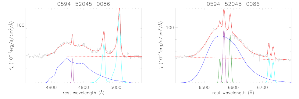
Figure 6: The accretion disk model determined best descriptions to the double-peaked broad H$\beta$ in the left panel and to the broad H$\alpha$ in the right panel. In the left panel, solid black line shows the line spectrum after subtractions of the optical Fe ii lines. In the right panel, solid black line shows the line spectrum. In each panel, solid red line shows the best descriptions to the emission lines by the elliptical accretion disk model plus multiple Gaussian functions, dashed red line shows the determined AGN continuum emissions underneath the emission lines, solid blue line shows the determined broad component from the disk-like emission regions, solid purple line shows the determined narrow Balmer line. In the left panel, solid cyan lines show the determined [O iii] doublet. In the right panel, solid lines in dark green and in cyan shows the determined [N ii] and [S ii] doublets. In order to show clearly determined broad Balmer emission lines, the Y-axis is in logarithmic coordinate.

In order to explain the double-peaked broad emission lines of AGN, besides the well described BBH model in the Introduction and well discussed in the following section, the proposed accretion disk origin has been well accepted. The accretion disk model is firstly proposed in Chen & Halpern (1989); Chen et al. (1989) to explain the double-peaked broad emission lines in AGN Arp102B and well applied in Eracleous & Halpern (1994). Then, different relativistic accretion disk models have been proposed in the literature, such as the improved elliptical accretion disk model in Eracleous et al. (1995), the circular disk model plus contributions of spiral arms in Storchi-Bergmann et al. (2003), the disk model with considerations of warped structures in Hartnoll & Blackman (2000), the stochastically perturbed accretion disk model in Flohic & Eracleous (2008), etc. Here, the elliptical accretion disk model (without contributions of subtle structures) well discussed in Eracleous et al. (1995) is preferred, because the model can be applied to well explain the double-peaked broad H$\beta$ in SDSS J1547. There are seven model parameters in the elliptical accretion disk model, inner boundary $r_{0}$ and out boundary $r_{1}$ in the units of $R_{g}$ (Schwarzschild radius), inclination angle $i$ of disk-like BLRs, eccentricity $e$, orientation angle $\phi_{0}$ of elliptical rings, local broadening velocity $\sigma_{L}$, line emissivity slope $q$ ($f_{r}~{}\propto~{}r^{-q}$). Meanwhile, we have also applied the very familiar elliptical accretion disk model, see our studies on double-peaked emission lines in Wang et al. (2005); Zhang (2011, 2013b, 2013a, 2015, 2021a). More detailed descriptions on the applied elliptical accretion disk model can be found in Eracleous et al. (1995); Storchi-Bergmann et al. (2003); Strateva et al. (2003), and there are no further descriptions on the elliptical accretion disk model in the manuscript. And the double-peaked broad H$\beta$ is described by the elliptical accretion disk model as follows.

Through the Levenberg-Marquardt least-squares minimization method, the emission lines can be described by the elliptical accretion disk model for the broad H$\beta$ plus multiple Gaussian functions for the narrow lines of narrow H$\beta$, core, broad and extremely extended components in the [O iii] doublets. When the elliptical accretion disk model is applied, the seven model parameters have restrictions as follows. The inner inner boundary $r_{0}$ is larger than 15${\rm R_{G}}$ and smaller than 1000${\rm R_{G}}$. The out boundary $r_{1}$ is larger than $r_{0}$ and smaller than $10^{6}{\rm R_{G}}$. The inclination angle $i$ of disk-like emission regions of broad H$\beta$ has $\sin(i)$ larger than 0.05 and smaller than 0.95. The eccentricity $e$ is larger than 0 and smaller than 1. The orientation angle $\phi_{0}$ of elliptical rings is larger than 0 and smaller than $2\pi$. The local broadening velocity $\sigma_{L}$ is larger than 10${\rm km/s}$ and smaller than $10^{4}{\rm km/s}$. And the line emissivity slope $q$ ($f_{r}~{}\propto~{}r^{-q}$) is larger than -7 and smaller than 7. The model parameters of the disk-like emission regions are about $r_{0}=163\pm 10{\rm R_{g}}$, $r_{1}=3265\pm 391{\rm R_{g}}$, $\sin(i)=0.293\pm 0.004$, $\sigma_{L}=175\pm 40{\rm km/s}$, $q=2.31\pm 0.06$, $e=0.621\pm 0.026$, $\phi_{0}=3.19$, respectively. The best descriptions to the double-peaked broad H$\beta$ is shown in the left panel of Figure 6 with $\chi^{2}\sim 1.01$.

Now considering probably different emission regions of broad H$\alpha$ from broad H$\beta$, it is interesting to check whether similar disk-like emission regions can be applied to explain the observed line profile of broad H$\alpha$. Here, the similar accretion disk model plus multiple Gaussian functions are applied, but the accretion disk model parameters of $r_{0}=163$, $\sin(i)=0.293$, $e=0.621$ and $\phi_{0}=3.19$ being fixed. The best descriptions to the broad H$\alpha$ is shown in the right panel of Figure 6 with $\chi^{2}\sim 1.91$. And the other three determined model parameters of the disk-like emission regions are about $r_{1}=2872\pm 250{\rm R_{g}}$, $\sigma_{L}=700\pm 50{\rm km/s}$, $q=1.72\pm 0.06$, respectively.

The accretion disk model can be well applied to described the different line profiles of broad Balmer emission lines, but the similar disk-like emission regions (similar boundaries, similar inclinations, similar eccentricity, etc.) for the broad H$\alpha$ and the broad H$\beta$ have much different local broadening velocities, which cannot be naturally expected. In one word, in order to overwhelm the expected double-peaked features in broad H$\alpha$, quite large local broadening velocity should be necessary in the emission regions of broad H$\alpha$. Unless there are quite different emission regions for the broad H$\alpha$ and the broad H$\beta$, the quite different broadening velocities can be not expected in emission regions of broad H$\alpha$ and broad H$\beta$. Therefore, the accretion disk origin is not preferred to explain the different line profiles of broad Balmer emission lines in SDSS J1547.

4 Two BLRs related to a central BBH system

Physical conditions have strong effects on intrinsic flux ratio of broad H$\alpha$ to broad H$\beta$, such as the previous results in Rees, Netzer & Ferland (1989); Korista & Goad (2004); Netzer (2020). In order to provide different physical conditions to broad Balmer line emission regions, two BLRs around central two black holes in a central BBH system should be well preferred. Intrinsic flux ratio of broad H$\alpha$ to broad H$\beta$ ($f_{\rm ab}$) in different physical conditions can be well varied from around 2 to around 4, such as the more recent discussed results in Netzer (2020). Now it is interesting to check whether varying $f_{\rm ab}$ from around 2 to around 4 can lead to different line profiles between Broad Balmer lines under the assumption of a central BBH system in SDSS J1547.

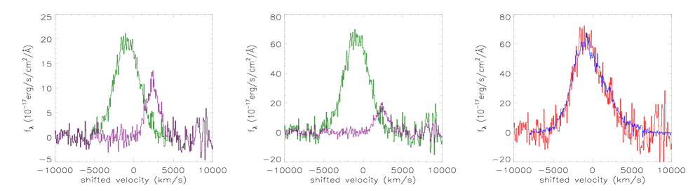
Figure 7: Left panel shows the two broad components in the broad H$\beta$: the blue-shifted broad component $F_{\rm Hb1}$ shown as solid dark green line and the red-shifted broad component $F_{\rm Hb2}$ shown as solid purple line. Middle panel shows the scaled broad components of $F_{\rm Hb1}\times 3.3$ and $F_{\rm Hb2}\times 1.5$. Right panel shows the expected line profile of the broad H$\alpha$ by $F_{\rm Hb1}\times 3.3+F_{\rm Hb2}\times 1.5$ shown as solid red line. And in right panel, solid blue line shows the observed line profile of the broad H$\alpha$ in SDSS J1547.

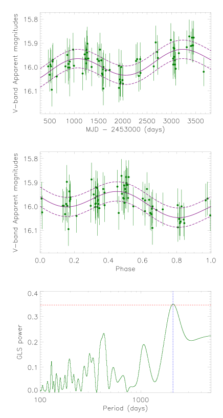
Figure 8: Top panel shows the long-term light curves from CSS (in dark green). Middle panel shows the corresponding phase folded light curve based on the determined periodicity about 2159days. In top and middle panels, solid and dashed lines in purple show the best descriptions to the light curve and the corresponding $1\sigma$ confidence bands, based on a sinusoidal function plus a linear trend. Bottom panel shows the Generalized Lomb-Scargle (GLS) periodogram. In bottom panel, horizontal dashed red line shows the 99.99% confidence level (0.0001 as the false-alarm probability), vertical blue line marks the peak around 2091days by the periodogram.

Not considering complicated structures, the two components are accepted from the broad H$\beta$: the blue-shifted broad component $F_{\rm Hb1}$ and the red-shifted broad component $F_{\rm Hb2}$, then, it is interesting to check whether two different flux ratios $f_{\rm ab}$ on $F_{\rm Hb1}$ and $F_{\rm Hb2}$ can lead to the similar line profile of the broad H$\alpha$. We can simply find that $f_{\rm ab}\sim 3.3$ on the blue-shifted broad component and $f_{\rm ab}\sim 1.5$ on the red-shifted broad component can lead to the similar line profile of the observed broad H$\alpha$. The results are shown in Figure 7. Here, $F_{\rm Hb1}$ and $F_{\rm Hb2}$ are similar as the smooth Gaussian components shown as solid dark green lines in Figure 2, but by the following formula

$$\begin{split}F_{\rm Hb1}&=F_{\lambda}-F_{\rm B2}-F_{\rm N}-pow\\ F_{\rm Hb2}&=F_{\lambda}-F_{\rm B1}-F_{\rm N}-pow\end{split}$$ (2)

where $F_{\lambda}$ means the line spectrum shown in Figure 2, $F_{\rm B1}$ means the determined blue-shifted broad Gaussian component in the broad H$\beta$, $F_{\rm B2}$ means the determined red-shifted broad Gaussian component in the broad H$\beta$, $F_{\rm N}$ means the sum of the determined narrow emission line components and $pow$ means the determined power-law component. Therefore, two BLRs with different physical conditions can be well applied to explain the observed different line profiles between the broad H$\alpha$ and the broad H$\beta$. Here, the different physical conditions include different ionization parameters, different electron temperatures, different electron densities, etc.. In the current stage, it is hard to determine which parameter has the key role on the different $f_{\rm ab}$ to the two BLRs in the central BBH system.

If the different line profiles of the broad Balmer emission lines were related to a central BBH system, the interesting features on the different line profiles could be detected in the candidates for BBH systems. Actually, there is really one BBH system reported with different line profiles of the broad Balmer emission lines in SDSS J0159+0105 as simply mentioned in Zheng et al. (2016). In SDSS J0159+0105, the red bump in the broad H$\beta$ is significant, but it is not very significant in the broad H$\alpha$, similar as the case in SDSS J1547.

Once accepted the central BBH system in SDSS J1547, it is interesting to check whether expected optical quasi-periodic oscillations (QPOs) can be detected in the long-term variabilities in SDSS J1547. The long-term V-band light curve has been collected from Catalina Sky Survey (CSS) (Drake et al., 2009) http://nesssi.cacr.caltech.edu/DataRelease/ with MJD-2453000 from 464 (April 2005) to 3644 (January 2014), and shown in top panel of Figure 8. Through the Levenberg-Marquardt least-squares minimization technique, the long-term CSS V-band light curve can be well described by a sinusoidal function plus a linear trend,

$$\begin{split}LMC&=(16.028\pm 0.019)-(0.018\pm 0.009)\times\frac{t}{\rm 1000days}\\ &+(0.044\pm 0.012)\sin(\frac{2\pi t}{2159\pm 210}+(1.725\pm 0.561))\end{split}$$ (3)

leading to the QPOs with periodicity about $2159\pm 210$ days. Meanwhile, based on the determined periodicity, the phase folded light curve is shown in the bottom panel of Figure 8, which can also be well described by a sinusoidal function. The results on the directed fitted results by the sinusoidal function and the phase folded light curve well described by a sinusoidal function strongly support the optical QPOs in SDSS J1547. However, the time duration of the CSS light curve is only 1.5times longer than the determined periodicity, leading the determined QPOs not to have high confidence levels. Future monitoring on SDSS J1547will be necessary to check the expected QPOs. Therefore, the Generalized Lomb-Scargle periodogram (Lomb, 1976; Scargle, 1982; Zechmeister & Kurster, 2009; Zheng et al., 2016) is applied and shown in bottom panel of Figure 8 with the clear peak around 2091days with confidence level higher than 99.99% well consistent with the determined $2159\pm 210$ days by the direct-fitting procedure, but no further discussions on the results from the periodogram.

Based on the different line profiles of the broad Balmer emission lines and the expected long-term optical QPOs, the BBH system can be well preferred as the first choice in SDSS J1547. Then, under the assumption of a BBH system, further properties of the BBH system can be simply discussed as follows. First, under the Virialization assumptions to the broad Balmer line emission clouds of each central BLRs (Peterson et al., 2004; Greene & Ho, 2005; Vestergaard & Peterson, 2006) combining with the more recent R-L relation discussed in Bentz et al. (2013):

$$\frac{M_{\rm BH}}{\rm M_{\odot}}=3.6\times 10^{6}\times(\frac{L_{\rm H\beta}}{\rm 10^{42}erg/s})^{0.56}\times(\frac{FWHM_{\rm H\alpha}}{\rm 1000km/s})^{2}$$ (4)

, based on the two apparent broad components in the broad H$\beta$, the virial BH masses of the two central BHs can be estimated as $M_{\rm BH,1}\sim 2.3\times 10^{7}{\rm M_{\odot}}$ and $M_{\rm BH,2}\sim 5.1\times 10^{6}{\rm M_{\odot}}$ for the blue-shifted BH accreting system and for the red-shifted BH accreting system, respectively. Second, based on the expected periodicity about 2159days combining with the estimated BH masses of the central BHs in a BBH system, the space separation of the two central BHs $A_{BBH}$ can be estimated as

$$A_{BBH}=0.432\times M_{8}\times(\frac{P_{BBH}/year}{2652M_{8}})^{2/3}\sim 0.005pc$$ (5)

where $M_{8}$ represents the total BH mass of the BBH system in unit of $10^{8}{\rm M_{\odot}}$ and $P_{BBH}\sim 5.92{\rm years}$ represents the orbital period of the BBH system in SDSS J1547. Third, based on the R-L relation in Bentz et al. (2013), expected BLRs size could be $R_{BLRs}\sim 25{\rm light-days}$ through the continuum luminosity at 5100Å  about $5.04\times 10^{43}{erg/s}$ in SDSS J1547. The very larger $R_{BLRs}\sim 25{\rm light-days}$ than the estimated $A_{BBH}\sim 5.8{\rm light-days}$ could probably rule out the existence of two totally distinctive BLRs in the central BBH system in SDSS J1547.

Before proceeding further, we simply discuss the larger $R_{BLRs}\sim 25{\rm light-days}$ than the estimated $A_{BBH}\sim 5.8{\rm light-days}$ in SDSS J1547  as follows. As discussed results in Shen & Loeb (2010), line profiles of broad emissions in BBHs systems are more complex, when the central two BLRs can no longer be distinct. However, in SDSS J1547, broad H$\alpha$ and broad H$\beta$ can be well described by two concise Gaussian components, providing weak signs of mixed two BLRs. The results probably indicate either $R_{BLRs}$ or $A_{BBH}$ is not so reliable in SDSS J1547. The R-L empirical relation determined from normal broad line AGN could not be well applied in BBHs systems. In the near future, further measurements on time lags between variabilities of broad Balmer emission lines and continuum emissions could provide more clearer results on sizes of broad Balmer line emission regions. Moreover, more accurate virial BH mass could also be estimated through multiple spectroscopic results. More efforts are necessary to determine more clearer properties of the expected BBH system in SDSS J1547.

5 How many AGN similar as SDSS J1547  can be found?

Before the end of the manuscript, it is interesting to consider the following question what percentage of broad line AGN can be expected to have very different line profiles of broad Balmer emission lines as indicators to central BBH system. Until now, SDSS J1547  is the only one object with reported detailed discussed different Balmer emission line profiles related to a central BBH. In the near future, it is necessary and interesting to detect more objects with very different line profiles of broad Balmer emission lines, and to check whether the objects could harbour central BBH systems. Here, the expected percentage can be estimated as follows. Once assumed central BBHs, the simple two broad Gaussian described components are accepted in the broad H$\beta$. Then, series of 20000 fake broad Balmer lines can be created by two steps. The blue-shifted broad Gaussian component $F_{H\beta,b}$ in the broad H$\beta$ has parameters of central wavelength randomly from -3000${\rm km/s}$ to 0${\rm km/s}$ in velocity space, second moment randomly from 800${\rm km/s}$ to 3000${\rm km/s}$ and line flux as 1 in arbitrary unit. And the red-shifted broad Gaussian component $F_{H\beta,r}$ in the broad H$\beta$ has parameters of central wavelength randomly from 0${\rm km/s}$ to 3000${\rm km/s}$ in velocity space, second moment randomly from 800${\rm km/s}$ to 3000${\rm km/s}$ and line flux randomly from 0.25 to 4 in arbitrary unit. The fake broad H$\beta$ can be created as $F_{H\beta,b}+F_{H\beta,r}$. Then, the fake two broad broad Gaussian components $F_{H\alpha,b}$ and $F_{H\alpha,r}$ in the velocity space are determined by $F_{H\alpha,b}=F_{H\beta,b}\times f_{\rm ab,b}$ and $F_{H\alpha,r}=F_{H\beta,r}\times f_{\rm ab,r}$ with $f_{\rm ab,b}$ and $f_{\rm ab,r}$ randomly from 1.5 to 4, leading the corresponding fake broad H$\alpha$ to be $F_{H\alpha,b}+F_{H\alpha,r}$.

Then, based on the fake broad Balmer lines, the line profiles of the fake broad Balmer lines can be well checked by properties of the three parameters: the absolute difference of central wavelength $\Delta\lambda_{0}$ between the broad H$\alpha$ and the broad H$\beta$, the absolute difference of second moment $\Delta\sigma$ between the broad H$\alpha$ and the broad H$\beta$, and the number of peaks $N_{\beta}$ and $N_{\alpha}$ in the broad H$\beta$ and the broad H$\alpha$. For the case in SDSS J1547, the determined values are $\Delta\lambda_{0,*}\sim 387{\rm km/s}$, $\Delta\sigma_{*}\sim 215{\rm km/s}$, $N_{\beta,*}=2$ and $N_{\alpha,*}=1$. Then, based on the criteria that $\Delta\lambda_{0}\geq\Delta\lambda_{0,*}$, $\Delta\sigma\geq\Delta\sigma_{*}$, $N_{\beta}=N_{\beta,*}$ and $N_{\alpha}=N_{\alpha,*}$, there are 25 cases with double-peaked broad H$\beta$ but single-peaked broad H$\alpha$, among the 20000 fake broad Balmer emission lines, indicating about 0.125% ($25/20000$) of broad line AGN having very different broad Balmer emission lines, similar as the case in SDSS J1547. Therefore, among the 13000 quasars in SDSS DR16 with redshift less than 0.35, there could be at least 16 quasars with very different broad Balmer emission lines. It will be worth to detect and check the SDSS quasars with very different line profiles of broad Balmer lines under the assumptions of central BBH systems in the near future.

6 Conclusions

Finally, we give our main conclusions as follows.

• Through the high quality SDSS spectra, very different broad Balmer emission lines can be confirmed in SDSS J1547: double-peaked broad H$\beta$ and broad H$\gamma$ but single-peaked broad H$\alpha$.

• The determined flux ratio of the narrow H$\alpha$ to the narrow H$\beta$ is larger than the ratio of the broad H$\alpha$ to the broad H$\beta$, indicating that rather than effects of dust obscurations, two BLRs related to a central BBH system are preferred in SDSS J1547. And the different physical conditions on the two expected central BLRs related to a central BBH system can be well applied to describe the very different broad Balmer emission lines in SDSS J1547.

• The long-term CSS V-band light curve of SDSS J1547  is checked. The light curve and the corresponding phase-folded light curve can be well described by a sinusoidal function, indicating probable QPOs with periodicity about $2159\pm 210$days expected by a central BBH system.

• The expected BBH system can be estimated with virial BH masses about $2.3\times 10^{7}{\rm M_{\odot}}$ and $5.1\times 10^{6}{\rm M_{\odot}}$ and with space separation about 0.005pc.

• Based on randomly created fake broad Balmer emission lines, about 0.125% of broad line AGN (quasars) have very different broad Balmer emission lines, similar as the case in SDSS J1547.

Data Availability

The data underlying this article will be shared on reasonable request to the corresponding author (xgzhang@njnu.edu.cn).

References

- Ahumada et al. (2020) Ahumada R., Prieto C. A., Almeida A.; et al., 2020, ApJS, 249, 3
- Begelman et al. (1980) Begelman, M. C.; Blandford, R. D.; Rees, M. J., 1980, Natur, 287, 307
- Bentz et al. (2010) Bentz, M. C.; Walsh J. L.; Barth, A., et al., 2010, ApJ, 716, 993
- Bentz et al. (2013) Bentz, M. C.; Denney, K. D.; Grier, C. J.; Barth, A. J.; Peterson, B. M., et al., 2013, ApJ, 767, 149
- Braibant et al. (2016) Braibant L., Hutsemekers D., Sluse D., Anguita T., 2016, A&A, 592, 23
- Brotherton et al. (2020) Brotherton, M. S.; Du, P.; Xiao, M.; Bao, D.; Zhao, B., et al., 2020, ApJ, 905, 77
- Brotherton et al. (2001) Brotherton, M. S.; Tran, H. D.; Becker, R. H.; Gregg, M. D.; Laurent-Muehleisen, S. A.; White, R. L.; et al., 2001, ApJ, 546, 775
- Chen & Halpern (1989) Chen, K.; Halpern, J. P., 1989, ApJ, 344, 115
- Chen et al. (1989) Chen, K.; Halpern, J. P., Filippenko, A. V., 1989, ApJ, 339, 742
- Cuadra et al. (2009) Cuadra, J.; Armitage, P. J.; Alexander, R. D.; Begelman, M. C., 2009, MNRAS, 393, 1423
- Di Matteo et al. (2005) Di Matteo, T., Springel, V., Hernquist, L. 2005, Natur, 433, 604
- De Rosa et al. (2018) De Rosa, G.; Fausnaugh, M. M.; Grier, C. J.; Peterson, B. M.; Denney, K. D.; et al., 2018, ApJ, 866, 133
- De Rosa et al. (2019) De Rosa, A.; Vignali, C.; Bogdanovic, T., et al., 2019, NewAR, 86, 101525
- Drake et al. (2009) Drake, A. J.; Djorgovski, S. G.; Mahabal, A., et al., 2009, ApJ, 696, 870
- Eracleous & Halpern (1994) Eracleous, Michael; Halpern, Jules P., 1994, ApJS, 90, 1
- Eracleous et al. (1995) Eracleous, M., Livio, M., Halpern, J. P., Storchi-Bergmann, T.,1995, ApJ, 438, 610
- Eracleous et al. (2005) Eracleous, M.; Livio, M.; Halpern, J. P.; Storchi-Bergmann, T., 1995, ApJ, 438, 610
- Flohic & Eracleous (2008) Flohic, H. M. L. G., & Eracleous, M., 2008, ApJ, 686, 138
- Gaskell (2009) Gaskell, C. M., 2009, NewAR, 53, 140
- Graham et al. (2015a) Graham, M. J.; Djorgovski, S. G.; Stern, D., et al., 2015a, Natur, 518, 74
- Graham et al. (2015b) Graham, M. J., Djorgovski, S. G., Stern, D., et al., 2015b, MNRAS, 453, 1562
- Greene & Ho (2005) Greene, J. E.; Ho, L. C., 2005, ApJ, 630, 122
- Grier et al. (2013) Grier, C. J.; Peterson, B. M.; Horne, Keith; Bentz, M. C.; Pogge, R. W., et al., 2013, ApJ, 764, 47
- Grier et al. (2017) Grier C. J., Pancoast A., Barth A. J., Fausnaugh M., Brewer B. J., Treu T., Peterson B. M., 2017, ApJ, 849, 146
- Gunn et al. (2006) Gunn, J. E., 2006, AJ, 131, 2332
- Hartnoll & Blackman (2000) Hartnoll, S. A.; Blackman, E. G., 2000, MNRAS, 317, 880
- Ho & Kim (2009) Ho, L. C.; Kim, M., 2009, ApJS, 184, 398
- Kaspi et al. (2000) Kaspi, S.; Smith, P. S.; Netzer, H.; Maoz, D.; Jannuzi, B. T.; Giveon, U., 2000, ApJ, 533, 631
- Khan et al. (2012) Khan, F.; Preto, M.; Berczik, P.; et al., 2012, ApJ, 749, 147
- Kovacevic et al. (2010) Kovacevic, J., Popovic, L. C., Dimitrijevic, M. S., 2010, ApJS, 189, 15
- Kollatschny & Zetzl (2013) Kollatschny W., Zetzl M., 2013, A&A, 549, 100
- Kollatschny et al. (2020) Kollatschny, W.; Weilbacher, P. M.; Ochmann, M. W.; Chelouche, D.; Monreal-Ibero, A.; Bacon, R.; Contini, T., 2020, A&A, 633, 79
- Liao et al. (2021) Liao, Wei-Ting; Chen, Yu-Ching; Liu, X.; et al., 2021, MNRAS, 500, 4025
- Liu et al. (2016) Liu, J., Eracleous, M., Halpern, J. P., 2016, ApJ, 817, 42
- Lomb (1976) Lomb, N. R. 1976, Ap&SS, 39, 447
- Rodriguez et al. (2009) Rodriguez, C., Taylor, G. B., Zavala, R. T., Pihlstrom, Y. M., Peck, A. B., 2009, ApJ, 697, 37
- Peterson et al. (2004) Peterson B. M., et al., 2004, ApJ, 613, 682
- Pfister et al. (2017) Pfister, Hugo; Lupi, Alessandro; Capelo, Pedro R.; et al., 2017, MNRAS, 371, 3646
- Sayeb et al. (2021) Sayeb, M.; Blecha, L.; Kelley, L. Z.; et al., 2021, MNRAS, 501, 2531
- Scargle (1982) Scargle, J. D. 1982, ApJ, 263, 835
- Shen & Loeb (2010) Shen, Y.; Loeb, A., 2010, ApJ, 725, 249
- Storchi-Bergmann et al. (2003) Storchi-Bergmann, T.; Nemmen da Silva, R.; Eracleous, M., et al., 2003, ApJ, 598, 956
- Storchi-Bergmann et al. (2017) Storchi-Bergmann, T.; Schimoia, J. S.; Peterson, B. M.; Elvis, M.; Denney, K. D.; Eracleous, M.; Nemmen, R. S., 2017, ApJ, 835, 236
- Strateva et al. (2003) Strateva, I. V., et al., 2003, AJ, 126, 1720
- Sulentic et al. (2000) Sulentic, J. W.; Marziani, P.; Dultzin-Hacyan, D., 2000, ARA&A, 38, 521
- Taniguchi & Wada (1996) Taniguchi, Y.; Wada, K., 1996, ApJ, 469, 581
- Vestergaard & Peterson (2006) Vestergaard, M., Peterson, B. M. 2006, ApJ, 641, 689
- Volonteri et al. (2003) Volonteri, M.; Haardt, F.; Madau, P., 2003, ApJ, 582, 559
- Korista & Goad (2004) Korista, K. T.; Goad, M. R., 2004, ApJ, 606, 749
- Netzer (2020) Netzer, H., 2020, MNRAS, 494, 1611
- Rees, Netzer & Ferland (1989) Rees, M. J.; Netzer, H.; Ferland, G. J., 1989, ApJ, 347, 640
- Vanden Berk et al. (2001) Vanden Berk, D. E.; Richards, G. T.; Bauer, A.; Strauss, M. A.; Schneider, D. P.; et al., 2001, ApJ, 122, 549
- Vietri et al. (2020) Vietri, G.; Mainieri, V.; Kakkad, D.; Netzer, H.; Perna, M.; et al., 2020, A&A, 644, 175
- Wang et al. (2005) Wang, T. G.; Dong, X. B.; Zhang, X. G., et al. 2005, ApJ Letter, 625, 35
- Zechmeister & Kurster (2009) Zechmeister, M.; Kurster, M., 2009, A&A, 496, 577
- Zhang (2011) Zhang, X. G., 2011, MNRAS, 416, 2857
- Zhang (2013a) Zhang, X. G., 2013a, MNRAS, 429, 2274
- Zhang (2013b) Zhang, X. G., 2013b, MNRAS Letter, 431, 112
- Zhang (2015) Zhang, X. G., 2015, MNRAS Letter, 447, 35
- Zhang (2021a) Zhang, X. G., 2015, MNRAS Letter, 500, 57
- Zhang (2021) Zhang, X. G., 2021, ApJ in press, arXiv:2101.02465
- Zheng et al. (2016) Zheng Z., Butler N. R., Shen Y., Jiang L., Wang J., Chen X., Cuadra, J., 2016, ApJ, 827, 56
- Zhou et al. (2004) Zhou, H., Wang, T., Zhang, X., Dong, X., Li, C. 2004, ApJL, 604, L33