The defocusing NLS equation with nonzero background: Large-time asymptotics in the solitonless region

Abstract

We consider the Cauchy problem for the defocusing Schr$\ddot{\text{o}}$dinger (NLS) equation with a nonzero background

$$iq_{t}+q_{xx}-2(|q|^{2}-1)q=0,$$

$$q(x,0)=q_{0}(x),\quad\lim_{x\to\pm\infty}q_{0}(x)=\pm 1.\$$

Recently, for the space-time region $|x/(2t)|<1$ which is a solitonic region without stationary phase points on the jump contour, Cuccagna and Jenkins presented the asymptotic stability of the $N$-soliton solutions for the NLS equation by using the $\bar{\partial}$ generalization of the Deift-Zhou nonlinear steepest descent method. Their large-time asymptotic expansion takes the form

$$q(x,t)=T(\infty)^{-2}q^{sol,N}(x,t)+\mathcal{O}(t^{-1}),$$ (0.1)

whose leading term is N-soliton and the second term $\mathcal{O}(t^{-1})$ is a residual error from a $\overline{\partial}$-equation. In this paper, we are interested in the large-time asymptotics in the space-time region $|x/(2t)|>1$ which is outside the soliton region, but there will be two stationary points appearing on the jump contour $\mathbb{R}$. We found a asymptotic expansion that is different from (0.1)

$$q(x,t)=e^{-i\alpha(\infty)}\left(1+t^{-1/2}h(x,t)\right)+\mathcal{O}\left(t^{-3/4}\right),$$ (0.2)

whose leading term is a nonzero background, the second $t^{-1/2}$ order term is from continuous spectrum and the third term $\mathcal{O}(t^{-3/4})$ is a residual error from a $\overline{\partial}$-equation. The above two asymptotic results (0.1) and (0.2) imply that the region $|x/(2t)|<1$ considered by Cuccagna and Jenkins is a fast decaying soliton solution region, while the region $|x/(2t)|>1$ considered by us is a slow decaying nonzero background region.
Keywords: defocusing NLS equation, Large-time asymtotics, Riemann-Hilbert problem, $\bar{\partial}$ steepest descent method.
Mathematics Subject Classification: 35Q51; 35Q15; 37K15; 35C20.

1 Introduction

In this paper, we study the Cauchy problem for the defocusing nonlinear Schr$\ddot{\text{o}}$dinger (NLS) equation on $\mathbb{R}\times\mathbb{R}_{+}$:

$$iq_{t}+q_{xx}-2(|q|^{2}-1)q=0,$$ (1.1)

$$q(x,0)=q_{0}(x),\quad\lim_{x\to\pm\infty}q_{0}(x)=\pm 1.$$ (1.2)

The NLS equation is one of the basic models in many branches of science, such as fibre optics, biology, physics, mathematics and social science [1, 2, 3, 4, 5, 6]. The Lax pair of the NLS equation was first derived by Zakharov and Shabat [7]; The well-posedness of the NLS equation with the initial data in Sobolev spaces $L^{2}(\mathbb{R})$ and $H^{s}(\mathbb{R}),\ s>0$ was proved by Tsutsumi and Bourgain respectively [8, 9]. The inverse scattering transform (IST) for the focusing NLS equation with zero boundary conditions was first developed by Zakharov and Shabat [10]. The next important step of the development of IST method is that the Riemann-Hilbert (RH) method, as the modern version of IST, was established by Zakharov and Shabat [11]. It has become clear that the RH method is applicable to construction of exact solutions and asymptotic analysis of solutions for a wide class of integrable systems [12, 13, 14, 15, 16, 17, 18, 19, 20, 21, 22].

We mention the following works on the long-time asymptotics of the defocusing NLS equation. For the initial data in the Schwarz space $\mathcal{S}(\mathbb{R})$ and using the IST method, Zakharov and Manakov obtained the long-time asymptotics of the NLS equation [23]

$$q(x,t)=t^{-1/2}h(x/t)e^{\frac{ix^{2}}{4t}\pm 2i|h(x/t)|^{2}\log t}+\mathcal{O}(t^{-3/2}),$$

with an arbitrary function $h(x)$. In 1981, Its presented a stationary phase method to analyze the long-time asymptotic behavior for the NLS equation [24]. In 1993, Deift and Zhou developed a nonlinear steepest descent method to rigorously obtain the long-time asymptotic behavior for the mKdV equation [25]. Later this method was extended to get the leading and high-order asymptotic behavior for the solution of the NLS equation (1.1) with the initial data $q_{0}(x)\in\mathcal{S}(\mathbb{R})$ [26, 27]

$$q(x,t)=t^{-1/2}\alpha(z_{0})e^{\frac{ix^{2}}{2t}-iv(z_{0})\log 4t}+\mathcal{O}(t^{-1}\log t).$$

Under much weaker weighted Sobolev initial data $q_{0}\in H^{1,1}(\mathbb{R})$, Deift and Zhou found the following result [28]

$$q(x,t)=t^{-1/2}\alpha(z_{0})e^{\frac{ix^{2}}{2t}-iv(z_{0})\log 4t}+\mathcal{O}(t^{-1/2-\kappa}),\ \ 0<\kappa<1/4.$$ (1.3)

In the serial of articles [29, 30, 31], Vartanian applied IST method to compute the leading and first correlation terms in the asymptotic behavior of the NLS equation with the finite density initial data $q_{0}(x)-q_{0}(\pm\infty)\in\mathcal{S}(\mathbb{R})$ as $x,t\to\pm\infty$ for both $|x/(2t)|>1$ (outside the soliton light cone) and $|x/(2t)|<1$ (inside the soliton light cone). In 2008, for $q_{0}\in H^{1,1}(\mathbb{R})$, Dieng and Mclaughlin applied the $\bar{\partial}$-steepest descent method to obtain a sharp estimate [32]

$$q(x,t)=t^{-1/2}\alpha(z_{0})e^{\frac{ix^{2}}{2t}-iv(z_{0})\log 4t}+\mathcal{O}(t^{-3/4}).$$

Jenkins investigated long-time/zero-dispersion limit of the solutions to the defocusing NLS equation associated to step-like initial data [33]

$$q(x,0)\sim\begin{cases}Ae^{-2i\mu x/\varepsilon},\quad x\to-\infty,\\ 1,\quad x\to\infty.\end{cases}$$

Fromm, Lenells and Quirchmayr studied the long-time asymptotics for the defocusing NLS equation with the step-like boundary condition [34]

$$q(x,t)\sim\begin{cases}\alpha e^{2i\beta x+i\omega t},\quad x\to-\infty,\\ 0,\quad x\to\infty.\end{cases}$$

Recently, for the finite density initial data $q_{0}(x)-\tanh x\in H^{4,4}(\mathbb{R})$, Cuccagna and Jenkins derived the leading order approximation to the solution of NLS equation in the solitonic space-time region I: $|\xi|<1$ with $\xi=x/(2t)$ by using $\bar{\partial}$ generalization of the Deift-Zhou nonlinear steepest descent method [35]

$$q(x,t)=T(\infty)^{-2}q^{sol,N}(x,t)+\mathcal{O}(t^{-1}),$$

whose leading term is N-soliton and the second term $\mathcal{O}(t^{-1})$ is a residual error from a $\overline{\partial}$-equation. See the region I in Figure 1. In our study, for the solitonless region II: $1<|\xi|,\ \xi=\mathcal{O}(1)$, we further obtain the large-time asymptotic behavior of the NLS equation (1.1)-(1.2) in the form

$$q(x,t)=e^{-i\alpha(\infty)}\left(1+t^{-1/2}h(x,t)\right)+\mathcal{O}\left(t^{-3/4}\right).$$

Compared to the results of Vartanian, see Theorem 2.2.1-2.2.2 in [30], we give a more holistic description of the solution as the parameters of a multi-soliton are modulated by soliton-soliton and soliton-radiation interactions. We also weaken the request on the initial data from the Schwartz space $\mathcal{S}(\mathbb{R})$ to a weighted Sobolev space $H^{4,4}(\mathbb{R})$. The $\bar{\partial}$-steepest descent method was first developed by McLaughlin and Miller to analyze the asymptotics of orthogonal polynomials with non-analytical weights [36, 37]. In recent years, this method has been successfully used to obtain the long-time asymptotics and the soliton resolution conjecture for some integrable systems [38, 39, 40, 41, 42].

Figure 1: The space-time region of $x$ and $t$, where the blue region I: $|\xi|<1$ which is solitonic region and was discussed by Cuccagna and Jenkins; the yellow regions II: $|\xi|>1,\ \xi=\mathcal{O}(1)$ which is solitonless region and we will consider in this paper.

Remark 1.1.

We consider the region $|\xi|>1,\ \xi=\mathcal{O}(1)$ due to the following reasons:

• This region for $|x|>2t$ as $t\to\infty$ was completely ignored by [35] and the long-time asymptotic behavior of the defocusing NLS in this region is still unknown.

• The above region also ensure that the phase point $\xi_{2}$ defined by (4.4) and (4.5) is bounded, such that subsequent estimates on ${\rm Re}(i\theta(z))$, the jump matrix and $\bar{\partial}$-derivatives are reasonable, see Proposition 4.1—5.2, Proposition 6.1—6.7, etc.

• For the case $|\xi|\rightarrow\infty$, we can derive the large-$x$ behavior of the NLS equation using the $\bar{\partial}$-steepest descent method.

• We will consider the transition space-time region $|x\pm 2t|=O(1)$ in the next study.

The structure of this work is as follows. In Section 2, we quickly recall the spectral analysis of the Lax pair which was obtained in [35], but is useful for our work. In Section 3, we list some important properties of the scattering data and the reflection coefficient, and formulate an RH problem for $M(z)$ to characterize the Cauchy problem (1.1)-(1.2). In Section 4 and Section 5, we make two deformations to the RH problem for $M(z)$. One is to regularize the RH problem and the other is to obtain a mixed $\bar{\partial}$-problem by continuous extensions of jump matrices. Then, we solve the mixed $\bar{\partial}$-problem by decomposing it into a pure RH problem and a pure $\bar{\partial}$-problem according to the $\bar{\partial}$-derivative. We give the detailed analysis on the pure RH problem and the pure $\bar{\partial}$-problem in Section 6 and Section 7 respectively. In Section 8, we calculate the large-time asymptotics for the NLS equation.

2 Spectral analysis on the Lax pair

To state our results, we give the following definition of normed spaces:

$$L^{p,s}(\mathbb{R}):=\{\mu(x)\in L^{p}(\mathbb{R})|\langle x\rangle^{s}\mu(x)\in L^{p}(\mathbb{R})\}\;\text{with}\;||\mu||_{L^{p,s}}:=||\langle x\rangle^{s}\mu||_{L^{p}},$$

$$W^{k,p}(\mathbb{R}):=\{\mu(x)\in L^{p}(\mathbb{R})|\partial^{j}\mu(x)\in L^{p}(\mathbb{R}),j=1,\cdots,k\}\;\text{with}\;||\mu||_{W^{k,p}}:=\sum_{j=0}^{k}||\partial^{j}\mu||_{L^{p}},$$

$$H^{k,s}(\mathbb{R}):=\{\mu(x)\in L^{2}(\mathbb{R})|\langle x\rangle^{s}\mu(x)\in L^{2}(\mathbb{R}),\langle y\rangle^{k}\hat{h}(y)\in L^{2}(\mathbb{R})\},$$

where $\langle x\rangle:=\sqrt{1+|x|^{2}}$ and $\hat{h}$ is the Fourier transform defined by

$$\hat{h}(y):=\frac{1}{2\pi}\int_{\mathbb{R}}e^{-ixy}h(x)\,\mathrm{d}x.$$

Below we give a quick review of the direct problem for the initial value problem (1.1)-(1.2). For details, see [35]. The NLS equation (1.1) admits a Lax pair

$$\psi_{x}=L\psi,\quad L=L(z;x,t)=i\sigma_{3}\left(Q-\lambda\left(z\right)\right),$$ (2.1)

$$\psi_{t}=T\psi,\quad T=T(z;x,t)=-2\lambda(z)L+i(Q^{2}-I)\sigma_{3}+Q_{x},$$ (2.2)

where

$$Q=Q(x,t)=\left(\begin{array}[]{cc}0&\bar{q}(x,t)\\ q(x,t)&0\end{array}\right),\quad\lambda(z)=\frac{z+z^{-1}}{2},\quad\sigma_{3}=\left(\begin{array}[]{cc}1&0\\ 0&-1\end{array}\right).$$

Replacing $L$ and $T$ by their limits as $x\to\pm\infty$, the Lax pair (2.1)-(2.2) changes to

$$\varphi_{x}^{\pm}=L_{\pm}\varphi^{\pm},\quad L_{\pm}=L_{\pm}(z;x,t)=i\sigma_{3}(Q_{\pm}-\lambda I),$$ (2.3)

$$\varphi_{t}^{\pm}=T_{\pm}\varphi^{\pm},\quad T_{\pm}=T_{\pm}(z;x,t)=-2\lambda L_{\pm},\ \ Q_{\pm}=\pm\sigma_{1}.$$ (2.4)

This spectral problem is easy to be solved with a solution

$$\varphi^{\pm} =Y_{\pm}e^{-it\theta(z)\sigma_{3}},\quad z\not=\pm 1,$$

$$\varphi^{\pm} =Y_{\pm},\quad z=\pm 1,$$

where

$$Y_{\pm}=I\pm\sigma_{1}/z,\quad\text{det}Y_{\pm}=1-z^{-2},$$ (2.5)

$$\theta(z)=\zeta(z)\big{(}x/t-2\lambda(z)\big{)},\quad\zeta(z)=(z-z^{-1})/2.$$ (2.6)

We define Jost solutions $\psi^{\pm}$ of Lax pairs (2.1)-(2.2) with the asymptotic behavior

$$\psi^{\pm}(z;x,t)\sim\varphi^{\pm}(z;x,t),\quad x\to\pm\infty.$$

Make a transformation

$$m^{\pm}(z;x,t)=\psi^{\pm}(z;x,t)e^{it\theta(z)\sigma_{3}},$$ (2.7)

then we have

$$m^{\pm}(z;x,t)\sim Y_{\pm},\quad x\to\pm\infty,$$ (2.8)

and a new Lax pair

$$(Y^{-1}_{\pm}m^{\pm})_{x}-i\zeta\left[Y^{-1}_{\pm}m^{\pm},\sigma_{3}\right]=Y^{-1}_{\pm}\Delta L_{\pm}m^{\pm},\quad z\not=\pm 1,$$ (2.9)

$$(Y^{-1}_{\pm}m^{\pm})_{t}+2i\zeta\lambda\left[Y^{-1}_{\pm}m^{\pm},\sigma_{3}\right]=Y^{-1}_{\pm}\Delta T_{\pm}m^{\pm},\quad z\not=\pm 1,$$ (2.10)

where $\Delta L_{\pm}=L-L_{\pm}$, $\Delta T_{\pm}=T-T_{\pm}$. The formula (2.9) can be converted into the integral equation: For $z\not=\pm 1$,

$$m^{\pm}(z;x)=Y_{\pm}+\int_{\pm\infty}^{x}\left[Y_{\pm}e^{-i\zeta(z)(x-y)\sigma_{3}}Y^{-1}_{\pm}\right]\left[\Delta L_{\pm}(z;y)m^{\pm}(z;y)\right]e^{i\zeta(z)(x-y)\sigma_{3}}\,\mathrm{d}y.$$ (2.11)

Then taking the limit of (2.11), we find as $z\to\pm 1$,

$$m^{\pm}(\pm 1;x)=Y_{\pm}+\int_{\pm\infty}^{x}\left[I+(x-y)L_{\pm}\right]\Delta L_{\pm}(z;y)m^{\pm}(z;y)\,\mathrm{d}y,$$ (2.12)

where we use the property that $\Delta L_{\pm}$ is sufficiently decayed. The existence, analyticity and differentiation of $m^{\pm}$ can be proven directly, here we just list their properties, for details, see [35].

Figure 2: The analytical region of $m(z)$: $m_{1}^{-}$ and $m_{2}^{+}$ are analytic in $\mathbb{C}^{+}$; $m_{1}^{+}$ and $m_{2}^{-}$ are analytic in $\mathbb{C}^{-}$.

Lemma 2.1.

Let $m^{\pm}_{j}(z;x),j=1,2$ be the column vector solutions of the equation (2.11). Given $n\in\mathbb{N}_{0}$ and $q\in\tanh(x)+L^{1,n}(\mathbb{R})$, $m_{1}^{+}(z;x)$ and $m_{2}^{-}(z;x)$ can be analytically extended to $z\in\mathbb{C}^{-}$. Similarly, $m_{1}^{-}(z;x)$ and $m_{2}^{+}(z;x)$ can be analytically extended to $z\in\mathbb{C}^{+}$ (See Figure 2). For any $x_{0}\in\mathbb{R}$, $m_{1}^{+}(z;x)$ and $m^{-}_{2}(z;x)$ are continuous differentiable maps defined on the lower half plane.

$$\partial^{n}_{z}m^{+}_{1}(z;x) :\overline{\mathbb{C}^{-}}\backslash\{-1,0,1\}\to C^{1}\big{(}[x_{0},\infty),\mathbb{C}^{2}\big{)}\cap W^{1,\infty}\big{(}[x_{0},\infty),\mathbb{C}^{2}\big{)},$$ (2.13)

$$\partial^{n}_{z}m_{2}^{-}(z;x) :\overline{\mathbb{C}^{+}}\backslash\{-1,0,1\}\to C^{1}\big{(}(-\infty,x_{0}],\mathbb{C}^{2}\big{)}\cap W^{1,\infty}\big{(}(-\infty,x_{0}],\mathbb{C}^{2}\big{)}.$$ (2.14)

Moreover, maps $q(x)\to\frac{\partial^{n}}{\partial z^{n}}m^{+}_{1}(z;x)$ and $q(x)\to\frac{\partial^{n}}{\partial z^{n}}m^{-}_{2}(z;x)$ are locally Lipschitz continuous from

$$\tanh(x)+L^{1,n}(\mathbb{R}) \to L^{\infty}_{loc}\left(\overline{\mathbb{C}^{-}}\backslash\{-1,0,1\},C^{1}\big{(}[x_{0},\infty),\mathbb{C}^{2}\big{)}\cap W^{1,\infty}\big{(}[x_{0},\infty),\mathbb{C}^{2}\big{)}\right),$$

$$\tanh(x)+L^{1,n}(\mathbb{R}) \to L^{\infty}_{loc}\left(\overline{\mathbb{C}^{-}}\backslash\{-1,0,1\},C^{1}\big{(}(-\infty,x_{0}],\mathbb{C}^{2}\big{)}\cap W^{1,\infty}\big{(}(-\infty,x_{0}],\mathbb{C}^{2}\big{)}\right).$$

Similar results hold for $q(x)\to m_{1}^{-}(z;x)$ and for $q(x)\to m_{2}^{+}(z;x)$.

In particular, there exists a function $F_{n}(\cdot)$, which is increasing and independent of $q$, such that

$$|\partial_{z}^{n}m^{+}_{1}(z;x)|\leq F_{n}\left(\left(1+|x|\right)^{n}||q-1||_{L^{1,n}(x,\infty)}\right),\quad z\in\overline{\mathbb{C}^{-}}\backslash\{-1,0,1\}.$$ (2.15)

Moreover, assume that $q(x)$ and $\tilde{q}(x)$ are sufficiently close and then we obtain

$$|\partial_{z}^{n}\left(m_{1}^{+}(z;x)-\tilde{m}_{1}^{+}(z;x)\right)|\leq||q-\tilde{q}||_{L^{1,n}(x,\infty)}F_{n}\left(\left(1+|x|\right)^{n}||q-1||_{L^{1,n}(x,\infty)}\right).$$ (2.16)

The other Jost functions also have similar statements.

We know from Lemma 2.1 that the Jost functions have singularities at points $-1$, $0$ and $1$. The following lemma shows that the singularity at the point $z=0$ can not be removed, but the singularities at points $z=\pm 1$ can be removed by improving the attenuation of the initial data.

Lemma 2.2.

Let $P$ be a compact support of $\{-1,1\}$ in $\overline{\mathbb{C}^{-}}\backslash\{0\}$. Then, for $q(x)\in L^{1,n+1}(\mathbb{R})+\tanh(x)$ where $n\in\mathbb{N}_{0}$ is fixed. There exists a constant $c$ such that for $z\in P$ we obtain

$$\left|m^{+}_{1}(z;x)-\left(\begin{array}[]{c}1\\ 1/z\end{array}\right)\right|\leq c\langle x^{-}\rangle e^{c\int_{x}^{\infty}\langle y-x\rangle|q(y)-1|\,\mathrm{d}y}||q-1||_{L^{1,1}(x,\infty)},$$ (2.17)

where $x^{-}=\text{max}\{-x,0\}$. Thus, we know the map $q\to m^{+}_{1}(z;\cdot)$ is locally Lipschitz continuous from

$$\tanh(x)+L^{1,1}(\mathbb{R})\to L^{\infty}\Big{(}\overline{\mathbb{C}^{-}}\backslash\{0\},C^{1}\big{(}[x_{0},\infty),\mathbb{C}^{2}\big{)}\cap W^{1,\infty}\big{(}[x_{0},\infty),\mathbb{C}\big{)}\Big{)}.$$ (2.18)

Furthermore, there exists a function $F_{n}(t)$, which is increasing and independent of $q$, such that

$$|\partial_{z}m^{+}_{1}(z)|\leq F_{n}\left((1+|x|)^{n+1}||q-1||_{L^{1,n+1}(x,\infty)}\right),\;z\in P.$$ (2.19)

The next lemma considers the asymptotics of the Jost functions as $z\to\infty$ and $z\to 0$.

Lemma 2.3.

Assume that $q(x)\in\tanh(x)+L^{1}(\mathbb{R})$ and $q^{\prime}(x)\in W^{1,1}(\mathbb{R})$. Then $m^{\pm}_{1}(z)$ and $m^{\pm}_{2}(z)$ have the following asymptotic behaviors:

$$m^{\pm}_{1}(z) =e_{1}+\mathcal{O}\left(z^{-1}\right);\ \ m^{\pm}_{2}(z)=e_{2}+\mathcal{O}\left(z^{-2}\right),z\to\infty,$$

$$m^{\pm}_{1}(z) =\pm\frac{e_{2}}{z}+\mathcal{O}(1);\ \ m^{\pm}_{2}(z)=\pm\frac{e_{1}}{z}+\mathcal{O}(1),\ \;z\to 0.$$

There exists an increasing function $F_{n}(t)$ for $q-\tanh(x)\in L^{1,n}(\mathbb{R})$ such that

$$|\partial_{z}^{j}m^{+}_{1}(z)|\leq|z|^{-1}F_{n}\left((1+|x|)^{n}||q-1||_{L^{1,n}(x,\infty)}\right),\;0\leq j\leq n,\;z\to\infty.$$ (2.20)

For any fixed two potential $q$ and $\tilde{q}$ which are sufficiently close to the other, we find

$$|\partial_{z}^{n}\left(m_{1}^{+}(z;x)-\tilde{m}_{1}^{+}(z;x)\right)|\leq|z|^{-1}||q-\tilde{q}||_{L^{1,n}(x,\infty)}F_{n}\left(\left(1+|x|\right)^{n}||q-1||_{L^{1,n}(x,\infty)}\right),$$ (2.21)

where $0\leq j\leq n$.

The Jost functions have the following symmetry.

Lemma 2.4.

Suppose that $q\in\tanh(x)+L^{1}(\mathbb{R})$. For $z\in\mathbb{C}\backslash\{-1,0,1\}$, we find

$$\psi_{\pm}(z;x)=\sigma_{1}\overline{\psi_{\pm}(\bar{z};x)}\sigma_{1}=\pm z^{-1}\psi^{\pm}(z^{-1};x)\sigma_{1}.$$ (2.22)

The above symmetry is expanded as follows according to matrix columns

$$\psi^{\pm}_{1}(z)=\sigma_{1}\overline{\psi^{\pm}_{2}(\bar{z})}=\pm z^{-1}\psi^{\pm}_{2}(z^{-1}),\;\psi^{\pm}_{2}(z)=\sigma_{1}\overline{\psi^{\pm}_{1}(\bar{z})}=\pm z^{-1}\psi^{\pm}_{1}(z^{-1}).$$ (2.23)

3 A RH problem with nonzero background

3.1 Scattering data and reflection coefficient

Since $\psi_{\pm}(z)$ are two matrix solutions of Lax pairs (2.1)-(2.2), there exists a spectral matrix

$$S(z)=\left(\begin{array}[]{cc}s_{11}(z)&s_{12}(z)\\ s_{21}(z)&s_{22}(z)\end{array}\right),$$

such that

$$\psi_{-}(z)=\psi_{+}(z)S(z),$$ (3.1)

where $s_{ij}(z)(i,j=1,2)$ are scattering data, by which we define a reflection coefficient

$$r(z):=\frac{s_{21}(z)}{s_{11}(z)}.$$ (3.2)

According to the lemma (2.4), the scattering data have the following properties [35]

Lemma 3.1.

Let $q\in\tanh(x)+L^{1}(\mathbb{R})$ and $z\in\mathbb{R}\backslash\{-1,0,1\}$. Then

• The scattering coefficients can be described by the Jost functions as

  $$s_{11}(z)=\frac{\det\left[\psi_{1}^{-}(z;x),\psi_{2}^{+}(z;x)\right]}{1-z^{-2}},\quad s_{21}(z)=\frac{\det\left[\psi_{1}^{+}(z;x),\psi_{1}^{-}(z;x)\right]}{1-z^{-2}}.$$ (3.3)

• $|s_{11}(z)|^{2}=1+|s_{21}(z)|^{2}\geq 1$, $z\in\mathbb{R}\backslash\{-1,0,1\}$.

• $|r(z)|^{2}=1-|s_{11}(z)|^{-2}<1$, $z\in\mathbb{R}\backslash\{-1,0,1\}$.

• For $z\in\mathbb{C}^{+}$,

  $$s_{11}(z)=-\overline{s_{11}\left(\bar{z}^{-1}\right)},\;s_{21}(z)=-\overline{s_{21}\left(\bar{z}^{-1}\right)},\;r(z)=\overline{r\left(\bar{z}^{-1}\right)}.$$ (3.4)

• If we add a condition $q^{\prime}\in W^{1,1}(\mathbb{R})$, then we can find, as $z\in\overline{\mathbb{C}^{+}}$,

  $$\lim_{z\to\infty}\left(s_{11}(z)-1\right)z=i\int_{\mathbb{R}}\left(|q(x)|^{2}-1\right)\,\mathrm{d}x,$$ (3.5)

  $$\lim_{z\to 0}\left(s_{11}(z)+1\right)z^{-1}=i\int_{\mathbb{R}}\left(|q(x)|^{2}-1\right)\,\mathrm{d}x,$$ (3.6)

  and as $z\in\mathbb{R}$

  $$|s_{21}(z)|=\begin{cases}\mathcal{O}\left(|z|^{-2}\right),\;|z|\to\infty,\\ \mathcal{O}\left(|z|^{2}\right),\;|z|\to 0,\end{cases}\quad r(z)\sim\begin{cases}z^{-2},\;|z|\to\infty,\\ 0,\;|z|\to 0.\end{cases}$$ (3.7)

• $s_{11}(z)$ and $s_{21}(z)$ both have simple poles at points $z=\pm 1$ and their residues at these points are proportional. Then, $z=\pm 1$ are the removable poles of $r(z)$.

  $$s_{11}(z)=\frac{s_{\pm}}{z\mp 1}+\mathcal{O}(1),\;s_{21}(z)=\mp\frac{s_{\pm}}{z\mp 1}+\mathcal{O}(1),\;\lim_{z\to\pm 1}r(z)=\mp 1,$$ (3.8)

  where $s_{\pm}$=$\frac{1}{2}\det\left[\psi_{1}^{-}(\pm 1;x),\psi_{2}^{+}(\pm 1;x)\right]$.

We consider the discrete spectrum relating to the initial value $q_{0}$, which is formed by a finite number of zeros of $s_{11}(z)$. Suppose that $z_{j}\in\mathbb{C}^{+}(j=1,\cdots,N)$ are the zeros of $s_{11}(z)$. Then, from the symmetries, we know $\bar{z}_{j}\in\mathbb{C}^{-}(j=1,\cdots,N)$ are the corresponding zeros of $s_{22}(z)$. The correlation $\mathcal{D}=\left\{r(z),\left(z_{j},c_{j}\right)^{N}_{j=1}\right\}$ is called the scattering data associated with the initial value $q_{0}$. With the above lemmas, we can prove

Lemma 3.2.

Let $q(x)\in\tanh(x)+L^{1,2}(\mathbb{R})$ and $q^{\prime}(x)\in W^{1,1}(\mathbb{R})$. Then we have

• $r(z)\in H^{1}(\mathbb{R})$.

• If $q_{0}\in\tanh(x)+H^{2,2}(\mathbb{R})$, the reflection coefficient meets

  $$||\log(1-|r|^{2})||_{L^{p}(\mathbb{R})}<\infty,\quad p\geq 1.$$ (3.9)

• $s_{11}(z)$ has no spectral singularity on the real axis and its zeros are simple, finite and distributed on the unit circle. For convenience, we define the corresponding discrete spectrum set

  $$\mathcal{Z}^{+}=\left\{z_{j}\in\mathbb{C}^{+}:s_{11}(z_{j})=0,z_{j}=e^{iw_{n}},0<w_{j}<\pi\right\},$$

  $$\mathcal{Z}^{-}=\left\{\bar{z}_{j}\in\mathbb{C}^{-}:s_{22}(\bar{z}_{j})=0,\bar{z}_{j}=e^{iw_{j}},-\pi<w_{j}<0\right\}.$$

Moreover, we can get the trace formula

$$s_{11}(z)=\prod_{j=1}^{N}\frac{z-z_{j}}{z-\bar{z}_{j}}\exp\left(-i\int_{\mathbb{R}}\frac{v(s)}{s-z}\,\mathrm{d}s\right),$$ (3.10)

where $z_{j}\in\mathcal{Z}^{+}$ and

$$v(s)=-\frac{1}{2\pi}\log\left(1-|r(s)|^{2}\right).$$ (3.11)

3.2 RH formulism of the initial value problem

Define

$$M(z)=M(z;x,t):=\begin{cases}\left(\frac{m_{1}^{-}(z;x,t)}{s_{11}(z)},m_{2}^{-}(z;x,t)\right),\;z\in\mathbb{C}^{+},\\[4.0pt] \left(m_{1}^{+}(z;x,t),\frac{m_{2}^{-}(z;x,t)}{\overline{s_{11}(\bar{z})}}\right),\;z\in\mathbb{C}^{-},\end{cases}$$ (3.12)

then it is easy to prove that $M(z)$ satisfies the following RH problem.

Figure 3: The jump contours and poles for $M(z)$. The black solid line stands for the jump line. The red dots are poles $z_{j},\ \bar{z}_{j}\ (j=1,\cdots,N)$, and the blue dots are singular points $-1,0,1$.

RHP1. Find a matrix-valued function $M(z)$ which satisfies

• Analyticity: $M(z)$ is meromorphic in $\mathbb{C}\backslash\mathbb{R}$.

• Symmetry: $M(z)=\sigma_{1}\overline{M(\bar{z})}\sigma_{1}=z^{-1}M(z^{-1})\sigma_{1}$.

• Jump condition: $M(z)$ satisfies the jump condition

  $$M_{+}(z)=M_{-}(z)V(z),\;z\in\mathbb{R},$$

  where

  $$V(z)=\left(\begin{array}[]{cc}1-|r(z)|^{2}&-e^{-2it\theta(z)}\overline{r(z)}\\ e^{2it\theta(z)}r(z)&1\end{array}\right),$$ (3.13)

  with $\theta(z)=\theta(z;x,t)=\zeta(z)[{x}/{t}-2\lambda(z)].$

• Asymptotic behaviors:

  $$M(z)=I+\mathcal{O}(z^{-1}),\quad z\to\infty,$$

  $$zM(z)=\sigma_{1}+\mathcal{O}(z),\quad z\to 0.$$

• Residue conditions: $M(z)$ has simple poles at each points $z_{j}$ in $\mathcal{Z}^{+}\cup\mathcal{Z}^{-}$ with the following residue conditions:

  $$\operatorname*{Res}_{z=z_{j}}M(z)=\lim_{z\to z_{j}}M(z)\left(\begin{array}[]{cc}0&0\\ c_{j}e^{2it\theta(z_{j})}&0\end{array}\right),$$ (3.16)

  $$\operatorname*{Res}_{z=\bar{z}_{j}}M(z)=\lim_{z\to\bar{z}_{j}}M(z)\left(\begin{array}[]{cc}0&\bar{c}_{j}e^{-2it\theta(\bar{z}_{j})}\\ 0&0\end{array}\right),$$ (3.19)

  where $c_{j}=\frac{s_{21}(z_{j})}{s^{\prime}_{11}(z_{j})}=iz_{j}|c_{j}|.$ The jump contours and poles of $M(z)$ can be seen in Figure 3.

Using the asymptotic property of $M(z)$ at infinity, we can obtain the reconstruction formula for the potential $q(x,t)$

$$q(x,t)=\lim_{z\to\infty}\left(zM(z;x,t)\right)_{21}.$$ (3.20)

4 Normalization of the RH problem

In this section, we make factorizations of the jump matrix $V(z)$ and renormalize the RH problem of $M(z)$ so that it is well-behaved at infinity.

4.1 Jump matrix factorizations

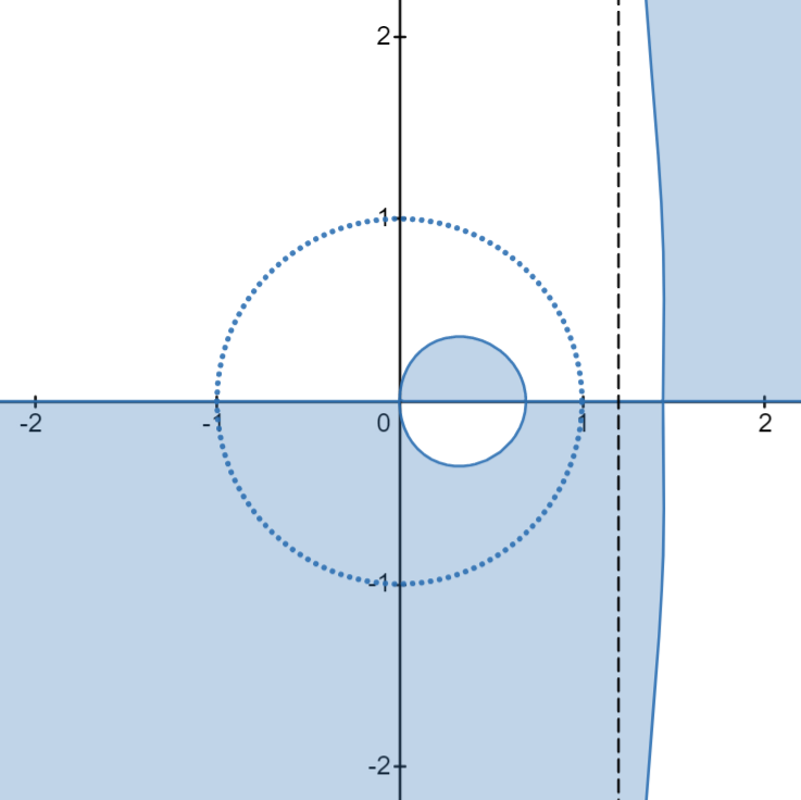
(a) $\xi>1$

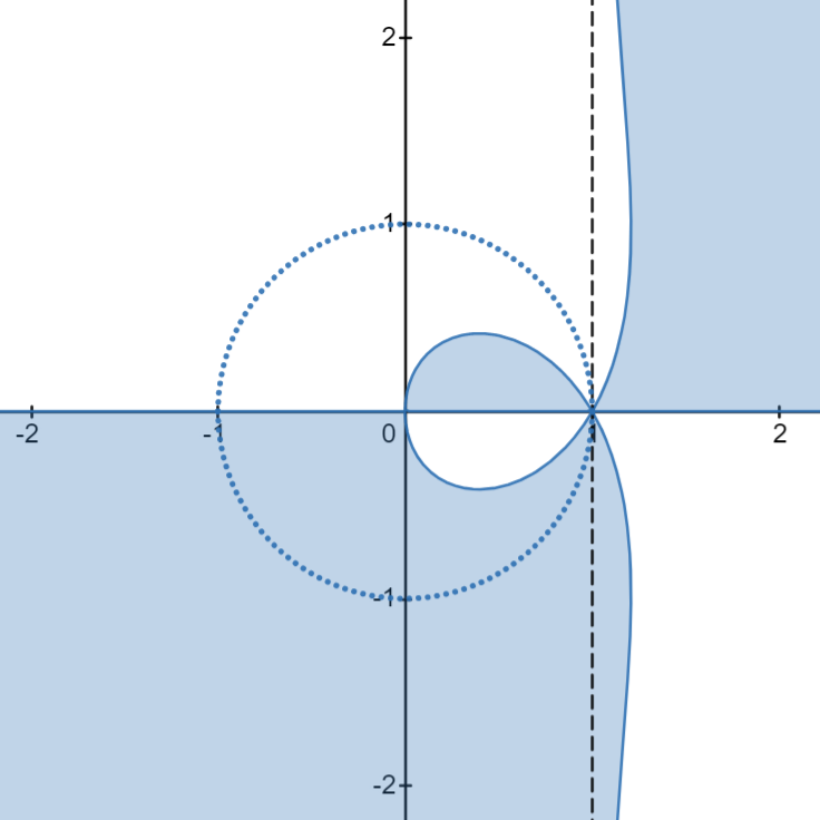
(b) $\xi=1$

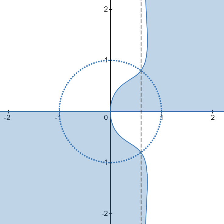
(c) $0<\xi<1$

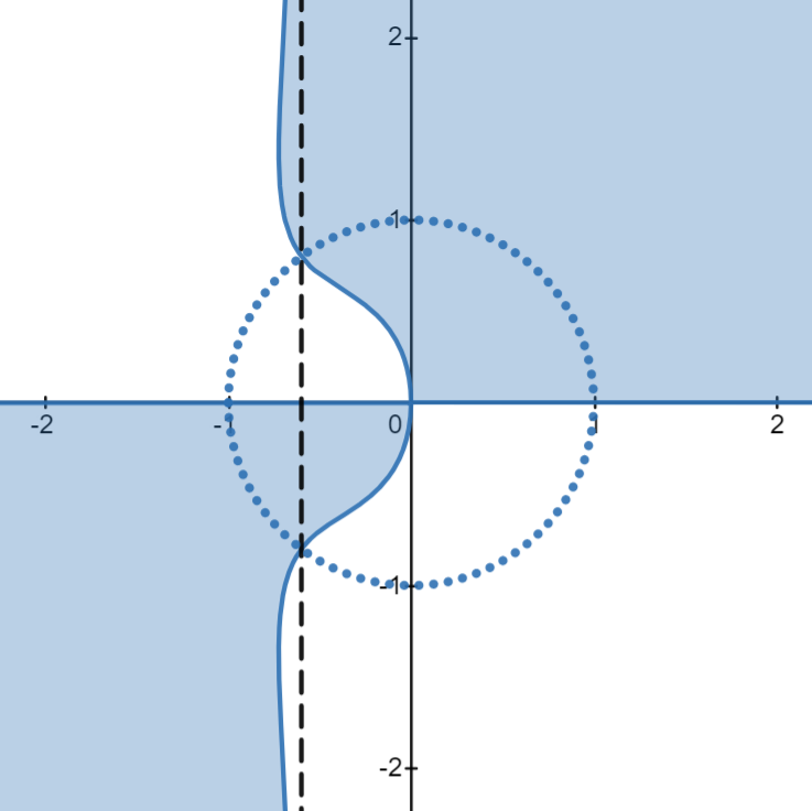
(d) $-1<\xi<0$

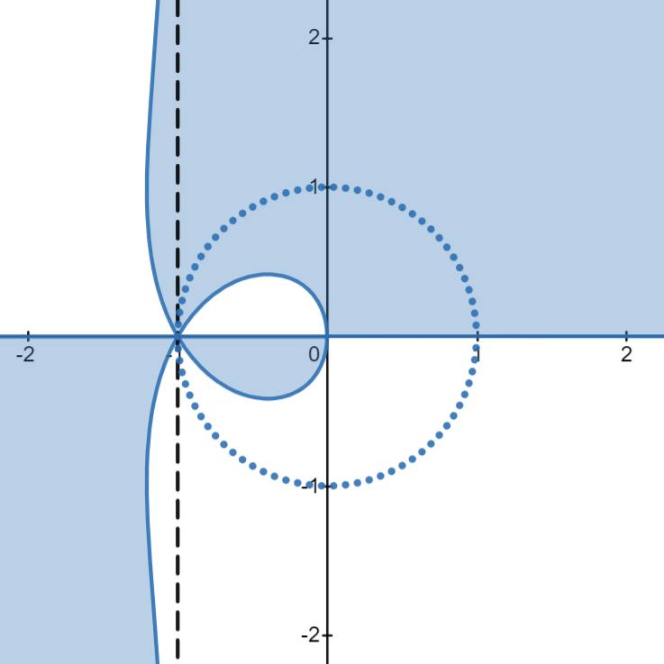
(e) $\xi=-1$

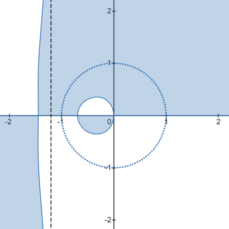
(f) $\xi<-1$

Figure 4: The signature table of $\operatorname*{Re}(2i\theta)$. In the blue region, we have $\operatorname*{Re}(2i\theta)>0$, which implies that $e^{-2it\theta}\to 0$ as $t\to\infty$; In the white region, $\operatorname*{Re}(2i\theta)<0$, which implies that $e^{2it\theta}\to 0$ as $t\to\infty$.

The long-time asymptotic behavior of RH problems is affected by growth and decay of the oscillatory term $e^{\pm 2it\theta(z)}$ in the jump matrix $V(z)$. Direct calculations show that

$$\operatorname*{Re}\left(2it\theta(z)\right)=\xi\operatorname*{Im}z\left(1+\frac{1}{\operatorname*{Re}^{2}z+\operatorname*{Im}^{2}z}\right)-\operatorname*{Re}z\operatorname*{Im}z\left(1+\frac{1}{\left(\operatorname*{Re}^{2}z+\operatorname*{Im}^{2}z\right)^{2}}\right),$$ (4.1)

where $\xi:=\frac{x}{2t}$. It can be found that the sign of $\operatorname*{Re}(2i\theta(z))$ changes with $\xi$. The signature table of $\operatorname*{Re}(2i\theta(z))$ is shown in Figure 4.

• For the case $|\xi|<1$, there is no phase point on $\mathbb{R}$ corresponding to the figures (c) and (d), which were discussed by Cuccagna and Jenkins [35];

• For the case $|\xi|=1$, there is a phase point on $\mathbb{R}$ corresponding to the figures (b) and (e), which are critical cases;

• For the case $|\xi|>1$, two phase points appear on $\mathbb{R}$, corresponding to the figures (a) and (f), which will be considered in our paper.

Next we search for stationary phase points of the function $\theta(z)$. Direct calculation gives

$$2\theta^{\prime}(z)=\frac{x}{t}\left(1+z^{-2}\right)-(2z+2z^{-3})=-2z^{-1}l(k),$$ (4.2)

$$2\theta^{\prime\prime}(z)=2z^{-2}l(s)-2z^{-1}l^{\prime}(s),$$ (4.3)

where $l(s)=s^{2}-\xi s-2,\quad s=z+z^{-1}$. We find (4.2) has two kinds of zeros on $\mathbb{R}$

$$\xi_{k}(\xi)=\frac{1}{2}\left|\nu(\xi)+(-1)^{k}\sqrt{\nu^{2}(\xi)-4}\right|,\quad k=1,2,\ \ {\rm for}\ \ \xi>1,$$ (4.4)

$$\xi_{k}(\xi)=-\frac{1}{2}\left|\nu(\xi)+(-1)^{k}\sqrt{\nu^{2}(\xi)-4}\right|,\quad k=1,2,\ \ {\rm for}\ \ \xi<-1,$$ (4.5)

where $\nu(\xi)=\frac{1}{2}(|\xi|+\sqrt{\xi^{2}+8})$. Based on the symmetry of zeros and the formula (4.4)-(4.5), we deduce that

$$\begin{cases}0<\xi_{1}(\xi)<1<\xi_{2}(\xi)\,\quad\xi>1,\\ \xi_{2}(\xi)<-1<\xi_{1}(\xi)<0\,\quad\xi<-1,\end{cases}$$ (4.6)

with $\theta^{\prime\prime}(\xi_{1}(\xi))>0\,\text{and}\,\theta^{\prime\prime}(\xi_{2}(\xi))<0$.

The jump matrix has the following two kinds of factorizations

$$V(z)=\begin{cases}\left(\begin{array}[]{cc}1&-\bar{r}e^{-2it\theta}\\ 0&1\end{array}\right)\left(\begin{array}[]{cc}1&0\\ re^{2it\theta}&1\end{array}\right),\\ \left(\begin{array}[]{cc}1&0\\ \frac{r}{1-|r|^{2}}e^{2it\theta}&1\end{array}\right)\left(\begin{array}[]{cc}1-|r|^{2}&0\\ 0&\frac{1}{1-|r|^{2}}\end{array}\right)\left(\begin{array}[]{cc}1&\frac{-\bar{r}}{1-|r|^{2}}e^{-2it\theta}\\ 0&1\end{array}\right).\end{cases}$$ (4.7)

Moreover, according to the signal of $\operatorname*{Re}(2i\theta(z))$, we use different factorization forms of the jump matrix for different regions such that the oscillating factor $e^{\pm 2it\theta}$ is decaying in the corresponding regions respectively.

Remark 4.1.

Here we only consider the zeros of the function $\theta(z)$ on $\mathbb{R}$, this is because for the zeros which on the complex plane but not on the junp curves $\Sigma$, they have no contribution to the solution of $M(z)$. If $\xi_{k}$ is a zero point of $\theta(z)$, then

• $\xi_{k}\notin\Sigma$: $M(z)$ is analytic at the point $\xi_{k}$. $\xi_{k}$ does not contribute to the solution of $M(z)$ and can therefore be ignored.

• $\xi_{k}\in\Sigma$: $M(z)$ is not analytic at the point $\xi_{k}$ and the exponential oscillation terms $e^{\pm 2it\theta}$ in the jump matrix slow down or smooth out around $\xi_{k}$. The contribution of jumps near $\xi_{k}$ to the solution of $M(z)$ is dominant.

4.2 Conjugation

We introduce a transformation to deform the jumps on the real axis to a path on which the oscillatory term decays exponentially. Denote

$$I(\xi)=\begin{cases}(0,\xi_{1})\cup\left(\xi_{2},\infty\right),\quad\xi>1,\\ (0,\infty)\cup\left(\xi_{2},\xi_{1}\right),\quad\xi<-1.\end{cases}$$ (4.8)

We define the following function:

$$T(z)=\exp\left(-i\int_{I(\xi)}v(s)\left(\frac{1}{s-z}-\frac{1}{2s}\right)\,\mathrm{d}s\right).\\$$ (4.9)

Proposition 4.1.

The function $T(z)$ has the following properties:

• Analyticity: $T(z)$ is analytical in $\mathbb{C}\backslash I(\xi)$.

• Symmetry: $\overline{T(\bar{z})}=T(z)^{-1}=T(z^{-1})$.

• Jump condition:

  $$T_{+}(z)=T_{-}(z)(1-|r(z)|^{2}),\quad z\in I(\xi).$$ (4.10)

• Asymptotic behavior: Let

  $$T(\infty):=\lim_{z\to\infty}T(z)=\exp\left(i\int_{I(\xi)}\frac{v(s)}{2s}\,\mathrm{d}s\right).$$ (4.11)

  Then, $|T(\infty)|=1$ and the asymptotic expansion at infinity is

  $$T(z)=T(\infty)\left(I+\frac{1}{2\pi iz}\int_{I(\xi)}\log(1-|r(s)|^{2})\,\mathrm{d}s+\mathcal{O}\left(z^{-2}\right)\right).$$ (4.12)

• Boundedness: The ratio $\frac{s_{11}(z)}{T(z)}$ is holomorphic in $\mathbb{C}^{+}$ and $\left|\frac{s_{11}(z)}{T(z)}\right|$ is bounded for $z\in\mathbb{C}^{+}$.

• Local properties: For $k=1,2$,

  $$|T(z)-T_{k}(\xi_{k})(z-\xi_{k})^{\epsilon_{k}v(\xi_{k})i}|\leq c||r||_{H^{1}}|z-\xi_{k}|^{1/2},\ \epsilon_{k}=(-1)^{k+1},$$ (4.13)

  where $z=\xi_{k}+\mathbb{R}^{+}e^{i\varphi_{k}},\,|\varphi_{k}|<\pi,$ and

  $$T_{k}(z)=T(\infty)e^{i\beta_{k}(z;\xi_{k})},\;\beta_{k}(z;\xi_{k})=\epsilon_{k}v(\xi_{k})\ln(z-\xi_{k})+\int_{I(\xi)}\frac{v(s)}{s-z}\,\mathrm{d}s.$$ (4.14)

Proof.

The first five properties of $T(z)$ are obvious, so we only give the proof for the local properties. We first prove the local property at the neighborhood of $\xi_{2}$ for $\xi>1$, and other cases can be proved in similar way. For $z=\xi_{2}+\mathbb{R}^{+}e^{i\varphi_{2}}$ ($|\varphi_{2}|<\pi$), $T(z)$ can be rewritten as

$$T(z) =T(\infty)\exp\left(-i\int_{\xi_{2}}^{+\infty}\frac{v(s)}{s-z}\,\mathrm{d}s\right)\exp\left(-i\int_{0}^{\xi_{1}}\frac{v(s)}{s-z}\,\mathrm{d}s\right)$$

$$=T(\infty)\left(z-\xi_{2}\right)^{iv_{2}}\exp\left(i\beta_{2}(z;\xi_{2})\right),$$ (4.15)

where $\beta_{2}(z;\xi_{2})$ is defined by (4.14). Then we estimate the error between $\beta_{2}(\xi_{2};\xi_{2})$ and $\beta_{2}(z;\xi_{2})$.

$$\begin{split}&\left|\beta_{2}(z;\xi_{2})-\beta_{2}(\xi_{2};\xi_{2})\right|\leq\left|v(\xi_{2})\ln(\xi_{2}+1-z)\right|+\left|\int_{\xi_{2}+1}^{+\infty}\frac{v(s)}{s-z}-\frac{v(s)}{s-\xi_{2}}\,\mathrm{d}s\right|\\ &+\left|\int_{\xi_{2}}^{\xi_{2}+1}\frac{v(s)-v(\xi_{2})}{s-z}-\frac{v(s)-v(\xi_{2})}{s-\xi_{2}}\,\mathrm{d}s\right|+\left|\int_{0}^{\xi_{1}}\frac{v(s)}{s-z}-\frac{v(s)}{s-\xi_{2}}\,\mathrm{d}s\right|.\end{split}$$ (4.16)

Through simple calculations, we know

$$v(\xi_{2})\ln(\xi_{2}+1-z)\sim-v(\xi_{2})(z-\xi_{2})+\mathcal{O}\left((z-\xi_{2})^{2}\right),$$ (4.17)

and

$$\left|\int_{\xi_{2}+1}^{+\infty}\frac{v(s)}{s-z}-\frac{v(s)}{s-\xi_{2}}\,\mathrm{d}s\right|\lesssim||r||_{H^{1}}|z-\xi_{2}|^{-1/2}.$$ (4.18)

Then, we have

$$\left|\int_{\xi_{2}}^{\xi_{2}+1}\frac{v(s)-v(\xi_{2})}{s-z}-\frac{v(s)-v(\xi_{2})}{s-\xi_{2}}\,\mathrm{d}s\right|,\ \left|\int_{0}^{\xi_{1}}\frac{v(s)}{s-z}-\frac{v(s)}{s-\xi_{2}}\,\mathrm{d}s\right|\lesssim||r||_{H^{1}}|z-\xi_{2}|^{-1/2}.$$

By combining (4.17) and (4.18), the inequality (4.13) can be obtained. ∎

4.3 Constructing interpolation functions

For all poles $z_{j}\in\mathcal{Z}^{+}$ on the unit circle $|z|=1$, we define

$$\rho=\frac{1}{2}\min\left(\operatorname*{min}\limits_{z_{j}\in\mathcal{Z}^{+}}|{\rm Im}z_{j}|,\ \operatorname*{min}\limits_{z_{k},z_{j}\in\mathcal{Z}^{+}}|z_{j}-z_{k}|,\operatorname*{min}\limits_{n=0,\pm 1}\{|\xi_{1}-n|,|\xi_{2}-n|\}\right).$$

If we make a small circle with each $z_{k}$ as its center point and $\rho$ as a radius respectively, then they are disjoint each other and real axis. See Figure 5. For convenience, we define a directed path

$$\Sigma^{pole}=\cup_{j=1}^{N}\left\{z\in\mathbb{C}:|z-z_{j}|=\rho\;or\;|z-\bar{z}_{j}|=\rho\right\}.$$ (4.19)

To convert the residues at $z_{k}$ into the corresponding jumps on circles such that they further decay on the new jumps, we introduce an interpolation function as follows.
For $\xi>1$,

$$G(z)=\begin{cases}\left(\begin{array}[]{cc}1&0\\ -\displaystyle{\frac{c_{j}e^{2it\theta(z_{j})}}{z-z_{j}}}&1\end{array}\right),\;|z-z_{j}|<\rho,\\[4.0pt] \left(\begin{array}[]{cc}1&-\displaystyle{\frac{\bar{c}_{j}e^{-2it\theta(\bar{z}_{j})}}{z-\bar{z}_{j}}}\\ 0&1\end{array}\right),\;|z-\bar{z}_{j}|<\rho,\\ \left(\begin{array}[]{cc}1&0\\ 0&1\end{array}\right),\;\text{as}\;z\;\text{in elsewhere};\end{cases}$$ (4.20)

for $\xi<-1$,

$$G(z)=\begin{cases}\left(\begin{array}[]{cc}1&-\displaystyle{\frac{z-z_{j}}{c_{j}e^{2it\theta(z_{j})}}}\\ 0&1\end{array}\right),\;|z-z_{j}|<\rho,\\[4.0pt] \left(\begin{array}[]{cc}1&0\\ -\displaystyle{\frac{z-\bar{z}_{j}}{\bar{c}_{j}e^{-2it\theta(\bar{z}_{j})}}}&1\end{array}\right),\;|z-\bar{z}_{j}|<\rho,\\ \left(\begin{array}[]{cc}1&0\\ 0&1\end{array}\right),\;\text{as}\;z\;\text{in elsewhere},\end{cases}$$ (4.21)

where $z_{j}\in\mathcal{Z}^{+}$ and the corresponding $\bar{z}_{j}\in\mathcal{Z}^{-}$. Then we make the following transformation which can renormalize the RH problem $M(z)$

$$M^{(1)}(z)=T(\infty)^{-\sigma_{3}}M(z)G(z)T(z)^{\sigma_{3}},$$ (4.22)

which satisfies the following RH problem.

RHP2. Find a matrix-valued function $M^{(1)}(z)=M^{(1)}(z;x,t)$ satisfying

• Analyticity: $M^{(1)}(z)$ is analytic in $\mathbb{C}\backslash\Sigma^{(1)}$ where $\Sigma^{(1)}=\mathbb{R}\cup\Sigma^{pole}$.

• Symmetry: $M^{(1)}(z)=\sigma_{1}\overline{M^{(1)}(\bar{z})}\sigma_{1}=z^{-1}M^{(1)}(z^{-1})\sigma_{1}$.

• Jump condition: $M^{(1)}_{+}(z)=M^{(1)}_{-}(z)V^{(1)}(z),$ where for $z\in\mathbb{R}$

  $$V^{(1)}(z)=\begin{cases}\left(\begin{array}[]{cc}1&-\bar{r}T^{-2}e^{-2it\theta}\\ 0&1\end{array}\right)\left(\begin{array}[]{cc}1&0\\ rT^{2}e^{2it\theta}&1\end{array}\right),\quad z\in\mathbb{R}\backslash I(\xi),\\ \left(\begin{array}[]{cc}1&0\\ \frac{r}{1-|r|^{2}}T_{-}^{2}e^{2it\theta}&1\end{array}\right)\left(\begin{array}[]{cc}1&\frac{-\bar{r}}{1-|r|^{2}}T_{+}^{-2}e^{-2it\theta}\\ 0&1\end{array}\right),\quad z\in I(\xi),\end{cases}$$ (4.23)

  while jump matrices on $z\in\Sigma^{pole}$ are given as follows.
  For $\xi>1,$

  $$V^{(1)}(z)=\begin{cases}\left(\begin{array}[]{cc}1&0\\ -\displaystyle{\frac{c_{j}T^{2}(z)e^{2it\theta(z_{j})}}{z-z_{j}}}&1\end{array}\right),\;|z-z_{j}|<\rho,\\[4.0pt] \left(\begin{array}[]{cc}1&\displaystyle{\frac{\bar{c}_{j}T^{-2}(z)e^{-2it\theta(\bar{z}_{j})}}{z-\bar{z}_{j}}}\\ 0&1\end{array}\right),\;|z-\bar{z}_{j}|<\rho.\end{cases}$$ (4.24)

  For $\xi<-1,$

  $$V^{(1)}(z)=\begin{cases}\left(\begin{array}[]{cc}1&-\displaystyle{\frac{z-z_{j}}{c_{j}T^{2}(z)e^{2it\theta(z_{j})}}}\\ 0&1\end{array}\right),\;|z-z_{j}|<\rho,\\[4.0pt] \left(\begin{array}[]{cc}1&0\\ \displaystyle{\frac{z-\bar{z}_{j}}{\bar{c}_{j}T^{-2}(z)e^{-2it\theta(\bar{z}_{j})}}}&1\end{array}\right),\;|z-\bar{z}_{j}|<\rho.\end{cases}$$ (4.25)

• Asymptotic behaviors:

  $$M^{(1)}(z)=I+\mathcal{O}(z^{-1}),\quad z\to\infty,$$

  $$zM^{(1)}(z)=\sigma_{1}+\mathcal{O}(z),\quad z\to 0.$$

5 Transition to a hybrid $\bar{\partial}$-RH problem

5.1 Opening the $\bar{\partial}$-lenses

Fix a sufficiently small angle $0<\phi(\xi)<\arctan\left(\frac{|\xi_{2}(\xi)|}{\min|\operatorname*{Im}z_{j}|}\right),j=1,\cdots,N$, such that all regions which are touched by opening the jump contour $\mathbb{R}$ do not intersect any pole point $z_{j}$. See Figure 5.

(a) $\xi>1$

(b) $\xi<-1$

Figure 5: The jump contours and the signal of $\operatorname*{Re}\left(2i\theta\right)$ in different regions for the two cases $\xi>1$ and $\xi<-1$: Open the jump contour $\mathbb{R}$ in a sufficient small fixed angle, such that the regions enclosed between the red and blue straight lines which contains the real lines does not touch any part of the circles of the poles. The signal $+$ means the real part $\operatorname*{Re}\left(2i\theta\right)>0$ in these regions, and $-$ stands for $\operatorname*{Re}\left(2i\theta\right)<0$ in the corresponding regions.

Denote $\xi_{0}=0$, $\xi_{0,1}=(\xi_{0}+\xi_{1})/2$, $\xi_{1,2}=(\xi_{1}+\xi_{2})/2$, and real intervals

$$l_{1}\in\left(0,|\xi_{0,1}|\sec\phi(\xi)\right),\ \ l_{2}\in\left(0,|\xi_{1,2}-\xi_{1}|\sec\phi(\xi)\right),$$

$$\tilde{l}_{1}\in\left(0,|\xi_{0,1}|\tan\phi(\xi)\right),\ \ \tilde{l}_{2}\in\left(0,|\xi_{1,2}-\xi_{1}|\tan\phi(\xi)\right).$$

Then we define the boundaries $\Sigma_{kj},\ k=0,1,2,\ j=1,2,3,4$, produced after opening the real axis $\mathbb{R}$ at $0,\xi_{1},\xi_{2}$:

$$\Sigma_{k1}=\xi_{k}+e^{i\phi(\xi)}\mathbb{R}^{+},\quad\Sigma_{k2}=\xi_{k}+e^{i\left(\pi-\phi(\xi)\right)}l_{2},\quad\Sigma_{k3}=\overline{\Sigma}_{k2},\quad\Sigma_{k4}=\overline{\Sigma}_{k1},\ k=0,2,$$

$$\Sigma_{11}=\xi_{1}+e^{i\left(\pi-\phi(\xi)\right)}l_{1},\quad\Sigma_{12}=\xi_{1}+e^{i\phi(\xi)}l_{2},\;\quad\Sigma_{13}=\overline{\Sigma}_{12},\quad\,\Sigma_{14}=\overline{\Sigma}_{11},$$

$$\Sigma^{\prime}=\cup_{j=1}^{4}\Sigma^{\prime}_{j},\ \ \Sigma^{\prime}_{1}=\xi_{0,1}+e^{i\pi/2}\tilde{l}_{1},\quad\Sigma^{\prime}_{2}=\overline{\Sigma}^{\prime}_{1},\quad\Sigma^{\prime}_{3}=\xi_{1,2}+e^{i\pi/2}\tilde{l}_{2},\quad\Sigma^{\prime}_{4}=\overline{\Sigma}^{\prime}_{3}.$$

Denote by $\Omega_{kj},k=0,1,2,j=1,2,3,4$, the twelve sectors enclosed between the boundaries $\Sigma_{kj}$ and the real line as shown in Figure 6. Denote the cone $\Omega=\cup_{k=0}^{2}\cup_{j=1}^{4}\Omega_{kj}$, and the intervals

$$I_{1}=\begin{cases}(-\infty,0),\text{for}\;\xi>1,\\ (-\infty,\xi_{2}),\text{for}\;\xi<-1,\end{cases}\;I_{2}=\begin{cases}(0,\xi_{1}),\text{for}\;\xi>1,\\ (\xi_{2},\xi_{1}),\text{for}\;\xi<-1,\end{cases}$$

$$I_{3}=\begin{cases}(\xi_{1},\xi_{2}),\text{for}\;\xi>1,\\ (\xi_{1},0),\text{for}\;\xi<-1,\end{cases}\quad\;I_{4}=\begin{cases}(\xi_{2},+\infty),\text{for}\;\xi>1,\\ (0,+\infty),\text{for}\;\xi<-1.\end{cases}$$

(a) $\xi>1$

(b) $\xi<-1$

Figure 6: The continuous extension regions. ${\rm Re}(2i\theta)>0$ in the blue regions and ${\rm Re}(2i\theta)<0$ in the gray regions.

Proposition 5.1.

For $|\xi|>1,\ \xi=\mathcal{O}(1)$, we have for $z=\xi_{k}+le^{iw}:=\xi_{k}+u+iv,k=0,1,2$,

$$\operatorname*{Re}(2i\theta(z))\geq c(\xi,\xi_{k})v>0,\quad z\in\Omega_{k1}\cup\Omega_{k3},$$ (5.1)

$$\operatorname*{Re}(2i\theta(z))\leq-c(\xi,\xi_{k})v<0,\quad z\in\Omega_{k2}\cup\Omega_{k4},$$ (5.2)

where $c(\xi,\xi_{k})$ is a constant.

Proof.

We take the case for $\Omega_{01}$ and $\Omega_{11}$ of $\xi>1,\ \xi=\mathcal{O}(1)$ as an example to prove the above proposition. Other cases can be proven in the similar method. For $z\in\Omega_{01}$, assume that $z=|z|e^{iw}$,

$$\operatorname*{Re}\left(2it\theta(z)\right) =\sin(2w)\left(|z|+|z|^{-1}\right)^{2}-\xi\sin(2w)\left(|z|+|z|^{-1}\right)\sec(w)-2\sin(2w)$$

$$=G(|z|)\sin(2w),$$

where $G(|z|)=F(|z|)^{2}-\xi\sec(w)F(|z|)-2$ and $F(z)=z+z^{-1}$. The two zeros of $G(|z|)$ are

$$F_{1}(|z|)=\frac{\xi\sec(w)-\sqrt{\xi^{2}\sec(w)^{2}+8}}{2},\;F_{2}(|z|)=\frac{\xi\sec(w)+\sqrt{\xi^{2}\sec(w)^{2}+8}}{2}.$$

Since $F(|z|)\geq 2$, we only consider the zero $F_{2}(|z|)$ and define the corresponding $|z|=F_{2}^{-1}\left(\frac{\xi\sec(w)+\sqrt{\xi^{2}\sec(w)^{2}+8}}{2}\right)$. A simple calculation shows that as the angle $w<\pi/4$, then we have $\xi\sec(w)+\sqrt{\xi^{2}\sec(w)^{2}+8}>4$ and $G(z)\geq G\left(F_{2}^{-1}\left(\frac{\xi\sec(w)+\sqrt{\xi^{2}\sec(w)^{2}+8}}{2}\right)\right)>0$. Thus, $\operatorname*{Re}\left(2it\theta(z)\right)$ can be estimated by

$$\operatorname*{Re}\left(2it\theta(z)\right)\geq G\left(F_{2}^{-1}\left(\frac{\xi\sec(w)+\sqrt{\xi^{2}\sec(w)^{2}+8}}{2}\right)\right)>0.$$

For $z\in\Omega_{11}$, assume that $z=\xi_{1}+le^{iw}:=\xi_{1}+u+iv$,

$$\operatorname*{Re}\left(2it\theta(z)\right)=v\left(\xi+\frac{\xi}{|z|^{2}}-u\left(1+\frac{1}{|z|^{4}}\right)\right)>v\left(\xi-1+\frac{\xi}{|z|^{2}}-\frac{1}{|z|^{4}}\right).$$ (5.3)

Let $\tau=|z|^{2}$ and

$$h(\tau)=\xi-1+\xi\tau^{-1}-\tau^{-2}.$$ (5.4)

$h^{\prime}(\tau)>0$ as $z\in(\xi_{0,1},\xi_{1})$, so we have $h(\tau)\geq h(|(\xi_{1}-\xi_{0,1})\sec(w)|^{2})>0$. Finally, we obtain

$$\operatorname*{Re}\left(2it\theta(z)\right)\geq\left(\xi-1+\xi\cos(w)^{2}|\xi_{1}-\xi_{1,0}|^{-2}-\cos(w)^{4}|\xi_{1}-\xi_{1,0}|^{-4}\right)v>0.$$

∎

5.2 The hybrid $\bar{\partial}$-RH problem and its decompositions

We make continuous extensions of the jump matrix $V^{(1)}(z)$ to remove the jump from $\mathbb{R}$.

Proposition 5.2.

We define functions $R_{kj}:\bar{\Omega}\to\mathbb{C},k=0,1,2,j=1,2,3,4$, which have the following boundary values:

$$R_{k1}=\begin{cases}\frac{\overline{r(z)}T_{+}(z)^{-2}}{1-|r(z)|^{2}},\quad z\in I_{2}\cup I_{4},\\ f_{k1}(z)=\frac{\overline{r(\xi_{k})}T_{k}(\xi_{k})^{-2}}{1-|r(\xi_{k})|^{2}}\left(z-\xi_{k}\right)^{2iv(\xi_{k})\epsilon_{k}},\quad z\in\Sigma_{k1},\end{cases}$$ (5.5)

$$R_{k2}=\begin{cases}r(z)T(z)^{2},\quad z\in I_{1}\cup I_{3},\\ f_{k2}(z)=r(\xi_{k})T_{k}(\xi_{k})^{2}\left(z-\xi_{k}\right)^{-2iv(\xi_{k})\epsilon_{k}},\quad z\in\Sigma_{k2},\end{cases}$$ (5.6)

$$R_{k3}=\begin{cases}\overline{r(z)}T(z)^{-2},\quad z\in I_{1}\cup I_{3},\\ f_{k3}(z)=\overline{r(\xi_{k})}T_{k}(\xi_{k})^{-2}\left(z-\xi_{k}\right)^{2iv(\xi_{k})\epsilon_{k}},\quad z\in\Sigma_{k3},\end{cases}$$ (5.7)

$$R_{k4}=\begin{cases}\frac{r(z)T_{-}(z)^{2}}{1-|r(z)|^{2}},\quad z\in I_{2}\cup I_{4},\\ f_{k4}(z)=\frac{r(\xi_{k})T_{k}(\xi_{k})^{2}}{1-|r(\xi_{k})|^{2}}\left(z-\xi_{k}\right)^{-2iv(\xi_{k})\epsilon_{k}},\quad z\in\Sigma_{k4},\end{cases}$$ (5.8)

where $r(\xi_{0})=r(0)=0$. Then there exists a constant $c_{1}$ such that for $\xi>1$,

$$|\bar{\partial}R_{kj}|\leq c_{1}\left(|r^{\prime}(\operatorname*{Re}(z))|+|z-\xi_{k}|^{-1/2}\right),\quad\text{for all $z\in\Omega_{kj}$};$$ (5.9)

for $\xi<-1$ with $k=0,2$,

$$|\bar{\partial}R_{kj}|\leq\begin{cases}c_{1}\left(|\varphi_{k}(\operatorname*{Re}(z))|+|r^{\prime}(\operatorname*{Re}(z))|+|z-\xi_{k}|^{-1/2}\right),\quad\text{for $z\in\Omega_{kj},j=1,4$},\\ c_{1}\left(|r^{\prime}(\operatorname*{Re}(z))|+|z-\xi_{k}|^{-1/2}\right),\quad\text{for $z\in\Omega_{kj},j=2,3$},\\ c_{1}|z+1|,\quad{\rm near}\ z=-1,\\ c_{1}|z-1|,\quad{\rm near}\ z=1,\end{cases}$$ (5.10)

where $\varphi_{k}(z)=\begin{cases}\varphi^{(-1)}(z),\;k=2,\\ \varphi^{(1)}(z),\;k=0,\end{cases}$ and $\varphi^{(-1)},\varphi^{(1)}\in C_{0}^{\infty}\left(\mathbb{R},\left[0,1\right]\right)$ with small support near $-1$ and $1$ respectively, and for $\xi<-1$ with $k=1$,

$$|\bar{\partial}R_{1j}|\leq c_{1}\left(|r^{\prime}(\operatorname*{Re}(z))|+|z-\xi_{1}|^{-1/2}\right),\quad\text{for all $z\in\Omega_{1j}$}.$$ (5.11)

Proof.

We only provide the detailed proof for $R_{21}$ under the assumption that $\xi<-1$ and $\xi=\mathcal{O}(1)$, other cases can be done in a similar way. For convenience, we define the function

$$g_{1}(z)=f_{21}T(z)^{2},\quad z\in\bar{\Omega}_{21}.$$

Observing the lemma (3.1), we find that $s_{11}(z)$ and $s_{21}(z)$ have singularities at $z=\pm 1$, and $\lim_{z\to\pm 1}r(z)=\mp 1$. This implies that $R_{21}$ is singular at $z=-1$, but the singularity can be balanced by the factor $T(z)^{-2}$. In fact, we can rewrite

$$\frac{\overline{r(z)}T_{+}(z)^{-2}}{1-|r(z)|^{2}}=\frac{\overline{s_{21}(z)}}{s_{11}(z)}\left(\frac{s_{11}(z)}{T_{+}(z)}\right)^{2}=\frac{\overline{J_{21}(z)}}{J_{11}(z)}\left(\frac{s_{11}(z)}{T_{+}(z)}\right)^{2}$$ (5.12)

where $J_{11}(z)=\det\left[\psi_{1}^{-}(z;x),\psi_{2}^{+}(z;x)\right]$ and $J_{21}(z)=\det\left[\psi_{1}^{+}(z;x),\psi_{1}^{-}(z;x)\right]$. Denote $\chi_{0},\chi_{-1}\in C^{\infty}_{0}\left(\mathbb{R},\left[0,1\right]\right)$ with a small support near $0$ and $-1$ respectively. Let $z-\xi_{2}=s_{2}e^{i\varphi_{2}}$ with $s_{2}>0$. For $z\in\bar{\Omega}_{21}$, the extension is given as follows:

$$R_{21}(z)=\hat{R}_{21}(z)+\tilde{R}_{21}(z),$$

$$\hat{R}_{21}(z)=\left(g_{1}(z)+\left(\frac{\overline{r(\operatorname*{Re}z)}}{1-|r(\operatorname*{Re}z)|^{2}}-g_{1}(z)\right)\cos(a_{0}\varphi_{2})\right)T(z)^{-2}\big{(}1-\chi_{-1}(\operatorname*{Re}z)\big{)},$$ (5.13)

$$\tilde{R}_{21}(z)=k(\operatorname*{Re}z)\frac{s^{2}_{11}(z)}{T^{2}(z)}\cos(a_{0}\varphi_{2})+\frac{i|z-\xi_{2}|}{a_{0}}\chi_{0}\left(\frac{\varphi_{2}}{\delta_{0}}\right)k^{\prime}(\operatorname*{Re}z)\frac{s^{2}_{11}(z)}{T^{2}(z)}\sin(a_{0}\varphi_{2}),$$ (5.14)

where $k(z):=\chi_{-1}(z)\frac{\overline{J_{21}(z)}}{J_{11}(z)}$, $a_{0}:=\frac{\pi}{2\phi(\xi)}$ and $\delta_{0}$ is a small positive constant.

Next, we calculate the $\bar{\partial}$-derivatives of (5.13)-(5.14). Since $\bar{\partial}=\frac{e^{i\varphi_{2}}}{2}\left(\partial_{s_{2}}+is_{2}^{-1}\partial_{\varphi_{2}}\right)$, we have

$$\begin{split}&\bar{\partial}\hat{R}_{21}=-\frac{\bar{\partial}\chi_{-1}(\operatorname*{Re}z)}{T(z)^{2}}\left(g_{1}(z)+\left(\frac{\overline{r(\operatorname*{Re}z)}}{1-|r(\operatorname*{Re}z)|^{2}}-g_{1}(z)\right)\cos(a_{0}\varphi_{2})\right)T(z)^{-2}\\ &+\bar{\partial}\left(g_{1}(z)+\left(\frac{\overline{r(\operatorname*{Re}z)}}{1-|r(\operatorname*{Re}z)|^{2}}-g_{1}(z)\right)\cos(a_{0}\varphi_{2})\right)T(z)^{-2}\big{(}1-\chi_{-1}(\operatorname*{Re}z)\big{)}.\end{split}$$ (5.15)

We can prove that

$$\left|\frac{\overline{r(\operatorname*{Re}z)}}{1-|r(\operatorname*{Re}z)|^{2}}-g_{1}(z)\right|\lesssim|z-\xi_{2}|^{1/2},$$ (5.16)

where we have used the Cauchy-Schwarz inequality. Let $\varphi^{(-1)}(z)\in C_{0}^{\infty}\left(\mathbb{R},\left[0,1\right]\right)$,

$$\varphi^{(-1)}(z)=\begin{cases}1,\;z\in\text{supp}\chi_{-1},\\ 0,\;\text{otherwise}.\end{cases}$$ (5.17)

Then, the first term in (5.15) can be bounded by $\varphi^{(-1)}(\operatorname*{Re}z)$. Therefore, the inequality

$$|\bar{\partial}R_{21}|\lesssim\varphi^{(-1)}(\operatorname*{Re}z)+|r^{\prime}(\operatorname*{Re}z)|+|z-\xi_{2}|^{-1/2},\quad\text{for}\;z\in\Omega_{21},$$ (5.18)

follows immediately.

As for $\tilde{R}_{21}(z)$,

$$\begin{split}\bar{\partial}\tilde{R}_{21}(z)&=\frac{1}{2}e^{i\varphi_{2}}s^{2}_{11}(z)T(z)^{-2}\Big{[}\cos(a_{0}\varphi_{2})k^{\prime}(s_{2})\left(1-\chi_{0}\left(\frac{\varphi_{2}}{\delta_{0}}\right)\right)-\frac{ia_{0}k(s_{2})}{s_{2}}\sin(a_{0}\varphi_{2})\\ &+\frac{i}{a_{0}}\left(s_{2}k^{\prime}(s_{2})\right)^{\prime}\sin(a_{0}\varphi_{2})\chi_{0}\left(\frac{\varphi_{2}}{\delta_{0}}\right)-\frac{1}{a_{0}\delta_{0}}k^{\prime}(s_{2})\sin(a_{0}\varphi_{2})\chi^{\prime}_{0}\left(\frac{\varphi_{2}}{\delta_{0}}\right)\Big{]}.\end{split}$$

We can easily to find that $|\bar{\partial}\tilde{R}_{21}(z)|\lesssim\varphi^{(-1)}(\operatorname*{Re}z)$. Thus, the result (5.10) can be obtained. ∎

Finally, we use $R^{(2)}(z)$ to make a new transformation

$$M^{(2)}(z)=M^{(1)}(z)R^{(2)}(z),$$ (5.19)

where for $z\in\Omega_{kj}(k=0,1,2)$,

$$R^{(2)}(z)=\begin{cases}\left(\begin{array}[]{cc}1&(-1)^{\tau}R_{kj}e^{-2it\theta}\\ 0&1\end{array}\right),\quad j=1,3,\\ \left(\begin{array}[]{cc}1&0\\ (-1)^{\tau}R_{kj}e^{2it\theta}&1\end{array}\right),\quad j=2,4,\end{cases}$$ (5.20)

with $\tau=\begin{cases}0,\;j=1,4,\\ 1,\;j=2,3,\end{cases}$ and for $z$ belongs to other regions, $R^{(2)}=I$. $M^{(2)}$ satisfies the following hybrid $\bar{\partial}$-problem.

$\bar{\partial}$-RHP. Find a matrix-valued function $M^{(2)}(z)=M^{(2)}(z;x,t)$ which satisfies

• Analyticity: $M^{(2)}(z)$ is continuous in $\mathbb{C}\setminus\Sigma^{(2)}$, where

  $$\Sigma^{(2)}=\cup_{j=1}^{4}\left(\left(\cup_{k=1}^{2}\Sigma_{kj}\right)\cup\Sigma^{\prime}_{j}\right)\cup\Sigma^{pole}.$$

• Jump condition:

  $$M^{(2)}_{+}(z)=M^{(2)}_{-}(z)V^{(2)}(z),$$ (5.21)

  where

  $$V^{(2)}(z)=\begin{cases}\left(\begin{array}[]{cc}1&-f_{kj}e^{-2it\theta}\\ 0&1\end{array}\right),\quad z\in\Sigma_{kj},\,j=1,3,\\ \left(\begin{array}[]{cc}1&0\\ f_{kj}e^{2it\theta}&1\end{array}\right),\quad z\in\Sigma_{kj},\,j=2,4,\\ \left(\begin{array}[]{cc}1&(f_{(k-1)j}-f_{kj})e^{-2it\theta}\\ 0&1\end{array}\right),\quad z\in\Sigma^{\prime}_{j},\,j=1,4,\\ \left(\begin{array}[]{cc}1&0\\ (f_{(k-1)j}-f_{ij})e^{2it\theta}&1\end{array}\right),\quad z\in\Sigma^{\prime}_{j},\,j=2,3,\\[3.0pt] V^{(1)}(z),\;z\in\Sigma^{{pole}},\end{cases}$$ (5.22)

  with $k=1,2$.

• Asymptotic behaviors:

  $$M^{(2)}(z)=I+\mathcal{O}(z^{-1}),\quad z\to\infty,$$

  $$zM^{(2)}(z)=\sigma_{1}+\mathcal{O}(z),\quad z\to 0.$$

• $\bar{\partial}$-derivative: For $z\in\mathbb{C}\setminus\Sigma^{(2)}$, we have

  $$\bar{\partial}M^{(2)}(z)=M^{(2)}(z)\bar{\partial}R^{(2)}(z),$$ (5.23)

  where

  $$\bar{\partial}R^{(2)}(z)=\begin{cases}\left(\begin{array}[]{cc}1&(-1)^{\tau}\bar{\partial}R_{kj}e^{-2it\theta}\\ 0&1\end{array}\right),\quad j=1,3,\\ \left(\begin{array}[]{cc}1&0\\ (-1)^{\tau}\bar{\partial}R_{kj}e^{2it\theta}&1\end{array}\right),\quad j=2,4,\end{cases}$$ (5.24)

  with $k=0,1,2$.

To solve $M^{(2)}(z)$, we decompose it into a pure RH problem $M^{(2)}_{RHP}(z)$ with $\bar{\partial}R^{(2)}(z)=0$ and a pure $\bar{\partial}$-problem $M^{(3)}(z)$ with

$$\bar{\partial}M^{(3)}(z)=M^{(3)}(z)W^{(3)}(z),$$

$$W^{(3)}(z)=M^{(2)}_{RHP}(z)\bar{\partial}R^{(2)}(z)M^{(2)}_{RHP}(z)^{-1}.$$

Next we analyze the two problems obtained by decomposition respectively.

6 Contribution from a pure RH problem

We first consider the following pure RH problem.

RHP3. Find a matrix-valued function $M^{(2)}_{RHP}(z)=M^{(2)}_{RHP}(z;x,t)$ which satisfies

• Analyticity: $M^{(2)}_{RHP}(z)$ is analytic in $\mathbb{C}\backslash\Sigma^{(2)}$.

• Jump condition:

  $$M^{(2)}_{RHP+}(z)=M^{(2)}_{RHP-}(z)V^{(2)}(z),$$ (6.1)

  where $V^{(2)}(z)$ is given by (5.22).

• Asymptotic behaviors: $M^{(2)}_{RHP}(z)$ has the same asymptotic behaviors with $M^{(2)}(z)$.

• $\bar{\partial}$-derivative: $\bar{\partial}R^{(2)}(z)=0,\quad z\in\mathbb{C}\backslash\Sigma^{(2)}.$

To separate out poles from the pure RH problem $M^{(2)}_{RHP}(z)$, we define

$$\mathcal{U}_{\xi}=\mathcal{U}_{\xi_{1}}\cup\mathcal{U}_{\xi_{2}},\ \ \ \mathcal{U}_{\xi_{k}}=\{z:|z-\xi_{k}|<\rho\},\ \ k=1,2.$$

In addition, the jump matrix $V^{(2)}(z)$ has the following estimation.

Proposition 6.1.

There exists a positive constant $c_{p}$ such that for $1\leq p\leq\infty$,

$$||V^{(2)}(z)-I||_{L^{p}(\Sigma^{(2)}\backslash\mathcal{U}_{\xi})}=\mathcal{O}\left(c_{p}e^{-c_{p}t}\right),\quad t\rightarrow\infty.$$ (6.2)

Proof.

We prove three cases for $z\in\Sigma_{21}\backslash\mathcal{U}_{\xi}$, $z\in\Sigma^{\prime}_{3}$ and $z\in\{z\in\mathbb{C}:|z-z_{1}|=\rho\}$ for $\xi>1$, and the other cases can be proved similarly. From the definition of $V^{(2)}$ and $R_{21}$, we have for $z\in\Sigma_{21}\backslash\mathcal{U}_{\xi}$ and $1\leq p<\infty$,

$$||V^{(2)}(z)-I||_{L^{p}(\Sigma_{21}\backslash\mathcal{U}_{\xi})}=||R_{21}e^{-2it\theta(z)}||_{L^{p}(\Sigma_{21}\backslash\mathcal{U}_{\xi})}\lesssim||e^{-2it\theta(z)}||_{L^{p}(\Sigma_{21}\backslash\mathcal{U}_{\xi})}.$$

Denote $z=\xi_{2}+le^{i\varphi}$, $l\in(\rho,\infty)$ for $z\in\Sigma_{21}\backslash\mathcal{U}_{\xi}$. Then the proposition 5.1 tells us $||e^{-2it\theta(z)}||^{p}_{L^{p}(\Sigma_{21}\backslash\mathcal{U}_{\xi})}\lesssim t^{-1}e^{-c_{p}t}$. For $z\in\Sigma^{\prime}_{3}$, then there exists a positive constant $l$ such that

$$||V^{(2)}(z)-I||_{L^{p}(\Sigma^{\prime}_{3})}=||(R_{22}-R_{12})e^{2it\theta(z)}||_{L^{p}(\Sigma^{\prime}_{3})}\lesssim||e^{2it\theta(z)}||_{L^{p}(\Sigma^{\prime}_{3})}\lesssim t^{-1/p}e^{-c_{p}t}.$$

For $z\in\{z\in\mathbb{C}:|z-z_{1}|=\rho\}$ under $\xi>1$,

$$||V^{(2)}(z)-I||_{L^{p}(\{z\in\mathbb{C}:|z-z_{1}|=\rho\})}=||c_{1}T^{2}(z)e^{2it\theta(z_{1})}(z-z_{1})^{-1}||_{L^{p}(\{z\in\mathbb{C}:|z-z_{1}|=\rho\})}$$

$$\lesssim C(\rho,p)||e^{2it\theta(z_{1})}||_{L^{p}(\{z\in\mathbb{C}:|z-z_{1}|=\rho\})}\lesssim C(\rho,p)e^{-c_{p}t},$$

where $C(\rho,p)$ is a positive constant. It is obvious that the estimation (6.2) is right when $p=\infty$ in the above cases. The other cases can be shown in a similar way.

∎

The proposition (6.1) tells us for $z\in\Sigma^{(2)}\backslash\mathcal{U}_{\xi}$ the jump matrix $V^{(2)}(z)$ uniformly goes to identity. Thus outside the $\mathcal{U}_{\xi}$ there is only exponentially small error by completely ignoring the jump condition of $M^{(2)}_{RHP}(z)$. Then, the pure RH problem $M_{RHP}^{(2)}(z)$ can be decomposed into two parts:

$$M^{(2)}_{RHP}(z)=\begin{cases}E(z)M^{out}(z),\quad z\in\mathbb{C}\backslash\mathcal{U}_{\xi},\\ E(z)M^{out}(z)M^{lo}(z),\quad z\in\mathcal{U}_{\xi},\end{cases}$$ (6.3)

where $M^{out}(z)$ is a solution by ignoring the jump conditions of $M^{(2)}_{RHP}(z)$ which has no discrete spectrum since we have transformed the information of poles to the jump condition, $M^{lo}(z)$ is a local model for phase points which matches with the parabolic cylinder model problem, and $E(z)$ is the error function which satisfies a small-norm RH problem.

6.1 The outer model

In this subsection, we consider the outer model $M^{out}(z)$. Since we have converted the poles to the jumps, there has no discrete spectrum in $M^{out}(z)$. In fact, in our situation, all discrete spectrums $z_{j}\ (j=1,\cdots,N)$ are away from the critical line $\operatorname*{Re}z=\xi$ , so the soliton contribution to the problem is exponentially small. This is because when the soliton is close to the critical line it will make the exponential term not decay, which is $e^{\pm 2it\theta(z_{j})}=\mathcal{O}(1)$, otherwise the exponential term will decay in the corresponding region. $M^{out}(z)$ satisfies the following RH problem.

RHP4. Find a matrix-valued function $M^{out}(z)=M^{out}(z;x,t)$ which satisfies

• Analyticity: $M^{out}(z)$ is analytic in $\mathbb{C}\backslash\{0\}$.

• Symmetry: $M^{out}(z)=\sigma_{1}\overline{M^{out}(\bar{z})}\sigma_{1}=z^{-1}M^{out}(z^{-1})\sigma_{1}$.

• Asymptotic behaviors:

  $$M^{out}(z)=I+\mathcal{O}(z^{-1}),\quad z\to\infty,$$

  $$zM^{out}(z)=\sigma_{1}+\mathcal{O}(z),\quad z\to 0.$$

Proposition 6.2.

The RHP4 exists a unique solution

$$M^{out}(z)=I+z^{-1}\sigma_{1}.$$ (6.4)

Proof.

$M^{out}(z)$ is analytic in $\mathbb{C}$ except for $z=0$. Making a transformation

$$\tilde{M}(z)=M^{out}(z)\left(I+z^{-1}\sigma_{1}\right)^{-1}.$$ (6.5)

Notice that

$$\left(I+z^{-1}\sigma_{1}\right)^{-1}=\left(1-z^{-2}\right)^{-1}\sigma_{2}\left(I+z^{-1}\sigma_{1}\right)^{T}\sigma_{2},$$ (6.6)

then we find that

$$\lim_{z\to 0}\tilde{M}(z) =\lim_{z\to 0}M^{out}(z)\left(I+z^{-1}\sigma_{1}\right)^{-1}=I,$$

$$\lim_{z\to\infty}\tilde{M}(z) =\lim_{z\to\infty}M^{out}(z)\left(I+z^{-1}\sigma_{1}\right)^{-1}=I.$$

$\tilde{M}(z)$ is bounded and analytic in the complex plane, so it is a constant matrix, which is $\tilde{M}(z)=I$. Finally, we obtain $M^{out}(z)=I+z^{-1}\sigma_{1}$.

∎

Remark 6.1.

The result here is a special case of the $m^{sol}_{j_{0}}$ in the paper [35] with $j_{0}=-1$ where the critical line $\operatorname*{Re}z=\xi$ is not passing through any neighborhood of the discrete spectra $z_{j}\in\mathcal{Z}$.

Outside the region $\mathcal{U}_{\xi}$, the error between $M^{(2)}_{RHP}(z)$ and $M^{out}(z)$ mainly comes from the contribution of neglecting the jump line and we will study the error in more detail in subsection 6.3. Before we consider the error function, we construct local models for the neighborhood of the phase points $\xi_{k}$ ($k=1,2$).

6.2 The local model

Denote local jump contours

$$\Sigma^{lo}:=\Sigma^{(2)}\cap\mathcal{U}_{\xi}=\Sigma_{1}\cup\Sigma_{2},$$

where $\Sigma_{k}:=\cup_{j=1}^{4}\Sigma_{kj}\cap\mathcal{U}_{\xi_{k}},\,k=1,2$. See Figure 7. Consider the following local RH problem:

(a)   $\xi>1$

(b)   $\xi<-1$

Figure 7: Jump contours $\Sigma^{lo}$ for $M^{lo}(z)$ corresponding to the cases $\xi>1$ and $\xi<-1$ respectively.

RHP5. Find a matrix-valued function $M^{lo}(z)=M^{lo}(z;x,t)$ such that

• Analyticity: $M^{lo}(z)$ is analytic in $\mathbb{C}\setminus\Sigma^{lo}$.

• Symmetry: $M^{lo}(z)=\sigma_{1}\overline{M^{lo}(\bar{z})}\sigma_{1}$.

• Jump condition: $M^{lo}_{+}(z)=M^{lo}_{-}(z)V^{(2)}(z),\quad z\in\Sigma^{lo}.$

• Asymptotic behavior: $M^{lo}(z)=I+\mathcal{O}(z^{-1}),\quad z\to\infty.$

This local RH problem, which consists of two local models on $\Sigma_{1}$ and $\Sigma_{2}$, has the jump condition and no poles. First, we show as $t\to\infty$, the interaction between $\Sigma_{1}$ and $\Sigma_{2}$ reduces to 0 to higher order and the contribution to the solution of $M^{lo}(z)$ is simply the sum of the separate contributions from $\Sigma_{1}$ and $\Sigma_{2}$.

We consider the trivial decomposition of the jump matrix

$$V^{(2)}(z)=b_{-}^{-1}b_{+},\ \ \;b_{-}=I,\ \ \;b_{+}=V^{(2)}(z),$$

$$w_{-}=0,\ \ w_{+}=V^{(2)}(z)-I,\ \ w=V^{(2)}(z)-I,$$

$$w=w_{1}+w_{2},\;w_{1}=0,z\in\Sigma_{2},\;w_{2}=0,z\in\Sigma_{1},$$

then

$$C_{w}f=C_{-}(fw_{+})+C_{+}(fw_{-})=C_{-}(f(V^{(2)}-I)),$$

where $C_{w}=C_{w_{1}}+C_{w_{2}}$ and $C_{\pm}$ is the Cauchy operator on $\Sigma^{(2)}$ defined by

$$C_{\pm}f(z)=\lim_{z^{\prime}\to z\in\Sigma^{(2)}}\frac{1}{2\pi i}\int_{\Sigma^{(2)}}\frac{f(s)}{s-z^{\prime}}\,\mathrm{d}s.$$ (6.7)

Then we have the following lemma.

Proposition 6.3.

$$||C_{w_{1}}C_{w_{2}}||_{L^{2}(\Sigma^{lo})}=||C_{w_{2}}C_{w_{1}}||_{L^{2}(\Sigma^{lo})}\lesssim t^{-1},$$ (6.8)

$$||C_{w_{1}}C_{w_{2}}||_{L^{\infty}(\Sigma^{lo})\to L^{2}(\Sigma^{lo})},||C_{w_{2}}C_{w_{1}}||_{L^{\infty}(\Sigma^{lo})\to L^{2}(\Sigma^{lo})}\lesssim t^{-1}.$$ (6.9)

Proof.

From the definition of the operators, we have for any $f\in L^{\infty}\cap L^{2}\left(\Sigma^{lo}\right)$,

$$C_{w_{1}}C_{w_{2}}f=C_{+}\left(C_{-}(fw_{2+})w_{1-}\right)+C_{-}\left(C_{+}(fw_{2-})w_{1+}\right).$$ (6.10)

Then,

$$||C_{-}\left(C_{+}(fw_{2-})w_{1+}\right)(\cdot)||_{L^{2}\left(\Sigma^{lo}\right)} =\Big{|}\Big{|}\int_{\Sigma_{1}}\left(\int_{\Sigma_{2}}\frac{f(\eta)w_{2-}(\eta)}{(\eta-\kappa)_{+}}\,\mathrm{d}\eta\right)\frac{w_{1+}(\kappa)}{(\kappa-\cdot)_{-}}\,\mathrm{d}\kappa\Big{|}\Big{|}_{L^{2}\left(\Sigma^{lo}\right)}$$

$$\lesssim||w_{1+}||_{L^{2}(\Sigma_{1})}\sup_{\kappa\in\Sigma_{1}}\Big{|}\int_{\Sigma_{2}}\frac{f(\eta)w_{2-}(\eta)}{\eta-\kappa}\,\mathrm{d}\eta\Big{|}.$$

Furthermore, we have $||w||_{L^{2}\left(\Sigma^{lo}\right)}\lesssim t^{-1/2}$. Combining the above two equations we can obtain the estimations (6.8)-(6.9) after direct calculations. ∎

Following the idea and step in [25], we can derive the proposition:

Proposition 6.4.

$$\int_{\Sigma^{lo}}\frac{(I-C_{w})^{-1}Iw}{s-z}\,\mathrm{d}s=\sum_{j=1}^{2}\int_{\Sigma_{j}}\frac{(I-C_{w_{j}})^{-1}Iw_{j}}{s-z}\,\mathrm{d}s+\mathcal{O}(t^{-3/2}).$$ (6.11)

We consider the Taylor expansion in the neighborhood of $\xi_{k},\ k=1,2$,

$$\theta(z)=\theta(\xi_{k})+\frac{\theta^{\prime\prime}(\xi_{k})}{2}(z-\xi_{k})^{2}+G_{k}(z;\xi_{k}),$$ (6.12)

where $G_{k}(z;\xi_{k})=\mathcal{O}\left((z-\xi_{k})^{3}\right)$. Then we obtain the following proposition.

Proposition 6.5.

Let $\xi=\mathcal{O}(1)$, define operators $N_{k}$ ($k=1,2$)

$$N_{k}:g(z)\to(N_{k}g)(z)=g\left(\frac{s}{\sqrt{2t\epsilon_{k}\theta^{\prime\prime}(\xi_{k})\epsilon_{k}}}+\xi_{k}\right),$$ (6.13)

where $s=u\xi_{k}e^{\pm i\varphi_{k}},\ |u|<\rho,\ k=1,2$. Then we have

$$\Big{|}\exp\left\{-itG_{k}\left(\frac{s}{\sqrt{2t\epsilon_{k}\theta^{\prime\prime}(\xi_{k})}}+\xi_{k};\xi_{k}\right)\right\}\Big{|}\to 1,\quad\text{as}\;t\to\infty.$$ (6.14)

Proof.

We only give the proof for $\xi_{1}$ and the proof for $\xi_{2}$ can be given similarly. The operator $N_{1}$ acting on $T^{-1}(z)e^{-it\theta(z)}$ in the neighborhood of $\xi_{1}$ gives

$$N_{1}\left(T^{-1}e^{-it\theta(z)}\right)=T^{-1}\left(\frac{s}{\sqrt{2t\theta^{\prime\prime}(\xi_{1})}}+\xi_{1}\right)\exp\left(-it\theta\left(\frac{s}{\sqrt{2t\theta^{\prime\prime}(\xi_{1})}}+\xi_{1}\right)\right).$$

Direct calculations show that

$$N_{1}\theta(z)=\theta(\xi_{1})+\frac{s^{2}}{4t}+G_{1}\left(\frac{s}{\sqrt{2t\theta^{\prime\prime}(\xi_{1})}}+\xi_{1};\xi_{1}\right),$$

$$N_{1}T^{-1}(z)=\left(2t\theta^{\prime\prime}(\xi_{1})\right)^{-\frac{v(\xi_{1})}{2}}e^{w\left(\frac{s}{\sqrt{2t\theta^{\prime\prime}(\xi_{1})}}+\xi_{1}\right)}s^{iv(\xi_{1})}\left(\frac{s}{\sqrt{2t\theta^{\prime\prime}(\xi_{1})}}+\xi_{1}-\xi_{2}\right)^{-iv(\xi_{2})},$$

where

$$w(z)=-\frac{1}{2\pi i}\int_{I(\xi)}\ln|s-z|\,\mathrm{d}\ln(1-|r|^{2}).$$ (6.15)

For $s=u\xi_{1}e^{\pm i\varphi_{1}}$, we can obtain the result (6.14) using direct calculations. ∎

Second, following the lemma 6.4, we introduce two local models $M^{lo,k}$ on the jump contour $\Sigma_{k}$ $(k=1,2)$ whose solutions can be given explicitly in terms of parabolic cylinder functions on the two contours respectively. We consider the following RH problems:

RHP6. Find a matrix-valued function $M^{lo,k}(z)=M^{lo,k}(z;\xi_{k},x,t)$ such that

• Analyticity: $M^{lo,k}(z)$ is analytic in $\mathbb{C}\backslash\Sigma_{k}$.

• Symmetry: $M^{lo,k}(z)=\sigma_{1}\overline{M^{lo,k}(\bar{z})}\sigma_{1}$.

• Jump condition:

  $$M^{lo,k}_{+}(z)=M^{lo,k}_{-}(z)V^{lo,k}(z),\quad z\in\Sigma_{k},$$

  where

  $$V^{lo,k}(z)=\begin{cases}\left(\begin{array}[]{cc}1&-f_{kj}e^{-2it\theta}\\ 0&1\end{array}\right),\,z\in\Sigma_{kj},j=1,3,\\ \left(\begin{array}[]{cc}1&0\\ f_{kj}e^{2it\theta}&1\end{array}\right),\,z\in\Sigma_{kj},j=2,4.\end{cases}$$ (6.16)

• Asymptotic behavior: $M^{lo,k}(z)=I+\mathcal{O}(z^{-1}),\quad z\to\infty.$

Here we take the construction of the model $M^{lo,1}(z)$ as an example, and the other cases can be considered similarly. In order to motivate this model, we define the rescaled local variable

$$s=s(z;\xi_{1})=\sqrt{2t\theta^{\prime\prime}(\xi_{1})}(z-\xi_{1}),$$ (6.17)

and we choose the branches of the logarithm with $-\pi<\arg s<\pi$. We set

$$r_{\xi_{1}}=-r(\xi_{1})T_{1}(\xi_{1})^{2}\exp\big{(}2it\theta(\xi_{1})+iv(\xi_{1})\log\left(2t\theta^{\prime\prime}(\xi_{1})\right)\big{)},$$ (6.18)

$$\tilde{\rho}=\tilde{\rho}(\xi_{1})=\sqrt{2t\theta^{\prime\prime}(\xi_{1})}\rho,\quad\tilde{\mathcal{U}}_{\xi_{1}}=\{s\in\mathbb{C}:|s|=\tilde{\rho}\},$$ (6.19)

where $|r_{\xi_{1}}|=|r(\xi_{1})|$. Making scaling transformation

$$M^{pc,1}(s;r_{\xi_{1}})=N_{1}M^{lo,1}(z),$$

where $s$ and $r_{\xi_{1}}$ satisfy the relations (6.17) and (6.18). After changing the variable we obtain the parabolic cylinder model problems.

RHP7. Find a matrix-valued function $M^{pc,1}(s;r_{\xi_{1}})=M^{pc,1}(s;r_{\xi_{1}},x,t)$ such that

• Analyticity: $M^{pc,1}(s;r_{\xi_{1}})$ is analytic in $\mathbb{C}\backslash\Sigma^{pc,1}$ where $\Sigma^{pc,1}=\cup_{j=1}^{4}\Sigma^{pc,1}_{j}$ with

  $$\Sigma^{pc,1}_{1}=\mathbb{R}^{+}e^{(\pi-\varphi)i}\cap\tilde{\mathcal{U}}_{\xi_{1}},\;\Sigma^{pc,1}_{2}=\mathbb{R}^{+}e^{\varphi i}\cap\tilde{\mathcal{U}}_{\xi_{1}},\;\Sigma^{pc,1}_{3}=\overline{\Sigma}^{pc,1}_{2},\;\Sigma^{pc,1}_{4}=\overline{\Sigma}^{pc,1}_{1}.$$

• Jump condition:

  $$M^{pc,1}_{+}(s;r_{\xi_{1}})=M^{pc,1}_{-}(s;r_{\xi_{1}})V^{pc,1}(s;r_{\xi_{1}}),\quad s\in\Sigma^{pc,1},$$

  where

  $$V^{pc,1}(s;r_{\xi_{1}})=\begin{cases}\left(\begin{array}[]{cc}1&\frac{-\bar{r}_{\xi_{1}}}{1-|r_{\xi_{1}}|^{2}}s^{2iv(\xi_{1})}e^{-is^{2}/2}\\ 0&1\end{array}\right),\,s\in\Sigma^{pc,1}_{1},\\ \left(\begin{array}[]{cc}1&0\\ r_{\xi_{1}}s^{-2iv(\xi_{1})}e^{is^{2}/2}&1\end{array}\right),\,s\in\Sigma^{pc,1}_{2},\\ \left(\begin{array}[]{cc}1&-\overline{r}_{\xi_{1}}s^{2iv(\xi_{1})}e^{-is^{2}/2}\\ 0&1\end{array}\right),\,s\in\Sigma^{pc,1}_{3},\\ \left(\begin{array}[]{cc}1&0\\ \frac{r_{\xi_{1}}}{1-|r_{\xi_{1}}|^{2}}s^{-2iv(\xi_{1})}e^{is^{2}/2}&1\end{array}\right),\,s\in\Sigma^{pc,1}_{4}.\end{cases}$$ (6.20)

• Asymptotic behavior:

  $$M^{pc,1}(s;r_{\xi_{1}})=I+\frac{M^{pc,1}_{1}(x,t)}{s}+\mathcal{O}\left(s^{-2}\right),\quad s\to\infty,$$

  where $M^{pc,1}_{1}(x,t)$ is the coefficient of the term $s^{-1}$ in $M^{pc,1}(s;r_{\xi_{1}})$.

Further, $M^{pc,1}(s;r_{\xi_{1}})$ can be constructed by the following transformation:

$$M^{pc,1}(s;r_{\xi_{1}})=\Psi(s;r_{\xi_{1}})P(s;r_{\xi_{1}})e^{is^{2}\sigma_{3}/4}s^{-iv(\xi_{1})\sigma_{3}},$$ (6.21)

where

$$P(s;r_{\xi_{1}})=\begin{cases}\left(\begin{array}[]{cc}1&0\\ -r_{\xi_{1}}&1\end{array}\right),\quad\arg s\in(0,\varphi),\\ \left(\begin{array}[]{cc}1&-\bar{r}_{\xi_{1}}\\ 0&1\end{array}\right),\quad\arg s\in(0,-\varphi),\\ \left(\begin{array}[]{cc}1&\frac{\bar{r}_{\xi_{1}}}{1-|r_{\xi_{1}}|^{2}}\\ 0&1\end{array}\right),\quad\arg s\in(\pi-\varphi,\pi),\\ \left(\begin{array}[]{cc}1&0\\ \frac{r_{\xi_{1}}}{1-|r_{\xi_{1}}|^{2}}&1\end{array}\right),\quad\arg s\in(-\pi,-\pi+\varphi),\end{cases}$$

and $\Psi(s,r_{\xi_{1}})$ satisfies the following RH problem:

RHP8. Find a matrix-valued function $\Psi(s;r_{\xi_{1}})$ which has the following properties:

• Analyticity: $\Psi(s;r_{\xi_{1}})$ is analytic in $\mathbb{C}\backslash\mathbb{R}$.

• Jump condition:

  $$\Psi_{+}(s;r_{\xi_{1}})=\Psi_{-}(s;r_{\xi_{1}})V^{\Psi}(0),\quad s\in\mathbb{R},$$

  where

  $$V^{\Psi}(0)=\left(\begin{array}[]{cc}1-|r_{\xi_{1}}|^{2}&\bar{r}_{\xi_{1}}\\ -r_{\xi_{1}}&1\end{array}\right).$$ (6.24)

• Asymptotic behavior:

  $$\Psi(s;r_{\xi_{1}})=\left(I+\frac{M^{pc,1}_{1}}{s}+\mathcal{O}(s^{-2})\right)s^{iv(\xi_{1})\sigma_{3}}e^{-is^{2}\sigma_{3}/4},\quad s\to\infty.$$

In a similar way [38, 40], this RH problem can be changed into a Weber equation to obtain its solution $\Psi(s;r_{\xi_{1}})=(\Psi_{jl})_{j,l=1}^{2}$ in terms of parabolic cylinder functions. Then using (6.21), we get the asymptotic solution of the RHP7. Further, we can obtain the asymptotic solution of $M^{pc,2}(s_{;}r_{\xi_{2}})$ similarly. The asymptotic results are shown in the following formula

$$M^{pc,k}(s_{;}r_{\xi_{k}})=I+\frac{M^{pc,k}_{1}}{s}+\mathcal{O}(s^{-2}),\quad s\to\infty,$$

where

$$M^{pc,k}_{1}=\left(\begin{array}[]{cc}0&-i\epsilon_{k}\beta_{12}^{\xi_{k}}\\ i\epsilon_{k}\beta_{21}^{\xi_{k}}&0\end{array}\right),$$ (6.27)

with

$$\beta_{12}^{\xi_{k}}=\frac{(2\pi)^{\frac{1}{2}}e^{\frac{(2k-1)\pi i}{4}}e^{\frac{-\pi\epsilon_{k}v(\xi_{k})}{2}}}{-r_{\xi_{k}}\Gamma(-i\epsilon_{k}v(\xi_{k}))},\ \;\beta_{12}^{\xi_{k}}\beta_{21}^{\xi_{k}}=v(\xi_{k}),\;\ \epsilon_{k}=(-1)^{k+1},$$

$$\arg\beta_{12}^{\xi_{k}}=\frac{(2k-1)\pi}{4}-\arg r_{\xi_{k}}+\arg\Gamma(i\epsilon_{k}v(\xi_{k})).$$

Remark 6.2.

From calculations above, we see that this asymptotic result (6.27) is independent of the opening fixed angle $\phi(\xi)$ satisfying $|\phi(\xi)|<\pi/4$.

Remark 6.3.

Noting that for the original RHP1, $M(z)$ admits the circular symmetry

$$M(z)=z^{-1}M(z^{-1})\sigma_{1}.$$ (6.28)

However for the local model RHP5, the matrix function $M^{lo}(z)$ no longer admits such circular symmetry as (6.28). So we cannot obtain the local model $M^{pc,1}(z)$ at the phase point $\xi_{1}$ through the local model $M^{pc,2}(z)$ at the symmetric phase point $\xi_{2}$ by means of circular symmetry. Therefore, we have to solve two local models separately since the local model cannot keep the circular symmetry like the symmetry with respect to the imaginary axis $i\mathbb{R}$.

6.3 The small-norm RH problem

Define the error function $E(z)$, which satisfies the following RH problem.

$$E(z)=\begin{cases}M^{(2)}_{RHP}(z)(M^{out})^{-1}(z),\quad z\in\mathbb{C}\backslash\mathcal{U}_{\xi},\\[3.0pt] M^{(2)}_{RHP}(z)(M^{lo}(z))^{-1}(M^{out})^{-1}(z),\quad z\in\mathcal{U}_{\xi}.\end{cases}$$ (6.29)

(a) The  region $\xi>1$

(b) The  region $\xi<-1$

Figure 8: The jump contour $\Sigma^{E}$ for the $E(z;\xi)$. The blue circles are $\mathcal{U}_{\xi_{k}}(k=1,2)$.

RHP9. Find a matrix-valued function $E(z)$ with the properties as follows:

• Analyticity: $E(z)$ is analytic in $\mathbb{C}\backslash\Sigma^{E}$,   where $\Sigma^{E}=\partial\mathcal{U}_{\xi}\cup\left(\Sigma^{(2)}\setminus\mathcal{U}_{\xi}\right).$

• Jump condition:

  $$E_{+}(z)=E_{-}(z)V^{E}(z),\quad z\in\Sigma^{E},$$

  where the jump matrix is given by

  $$V^{E}(z)=\begin{cases}M^{out}(z)V^{(2)}(z)(M^{out})^{-1}(z),\quad z\in\Sigma^{(2)}\backslash\mathcal{U}_{\xi},\\[3.0pt] M^{out}(z)M^{lo}(z)(M^{out})^{-1}(z),\quad z\in\partial\mathcal{U}_{\xi}.\end{cases}$$ (6.30)

  See Figure 8.

• Asymptotic behavior: $E(z)=I+\mathcal{O}(z^{-1}),\quad z\to\infty.$

Then we estimate the jump matrix of $E(z)$.

Proposition 6.6.

$$|V^{E}(z)-I|=\begin{cases}\mathcal{O}(e^{-c_{\rho}t}),\quad z\in\Sigma^{(2)}\backslash\mathcal{U}_{\xi},\\ \mathcal{O}(t^{-1/2}),\quad z\in\partial\mathcal{U}_{\xi}.\end{cases}$$ (6.31)

Proof.

Since $M^{out}$ is bounded, we have for $z\in\Sigma^{(2)}\backslash\mathcal{U}_{\xi}$,

$$|V^{E}(z)-I|\lesssim|V^{(2)}(z)-I|\lesssim e^{-c_{\rho}t},$$ (6.32)

and for $z\in\partial\mathcal{U}_{\xi_{k}}$,

$$|V^{E}(z)-I|\lesssim|M^{lo,k}(z)-I|\lesssim t^{-1/2}.$$

∎

According to Beal-Cofiman theory, we decompose $V^{E}(z)=(b_{-})^{-1}b_{+},$ with

$$b_{-}=I,\;b_{+}=V^{E},\ \ w_{-}=0,\;w_{+}=V^{E}-I.$$

Let $C_{w}$ be an integral operator: $L^{2}(\Sigma^{E})\to L^{2}(\Sigma^{E})$

$$C_{w}f=C_{-}\left(f\left(V^{E}-I\right)\right),$$ (6.33)

where $C_{-}$ is the Cauchy projection operator on $\Sigma^{E}$ defined by

$$C_{-}f(z)=\lim_{z^{\prime}\to z\in\Sigma^{E}}\frac{1}{2\pi i}\int_{\Sigma^{E}}\frac{f(s)}{s-z^{\prime}}\,\mathrm{d}s.$$ (6.34)

Then $||C_{w}||_{L^{2}(\Sigma^{E})}=\mathcal{O}(t^{-1/2})$ and the RHP9 exists a unique solution

$$E(z)=I+\frac{1}{2\pi i}\int_{\Sigma^{E}}\frac{\mu(s)\left(V^{E}-I\right)}{s-z}\,\mathrm{d}s,$$

where $\mu\in L^{2}\left(\Sigma^{E}\right)$ satisfies $\left(I-C_{w}\right)\mu=I$. Moreover, we can derive

$$||\mu-I||_{L^{2}(\Sigma^{E})}=\mathcal{O}(t^{-1/2}),\quad||V^{E}-I||_{L^{2}(\Sigma^{E})}=\mathcal{O}(t^{-1/2}).$$ (6.35)

In order to reconstruct the solution $q(x,t)$, we need the large-$z$ behavior of $E(z)$. We consider

$$E(z)=I+\frac{E_{1}}{z}+\mathcal{O}\left(z^{-1}\right),$$ (6.36)

where

$$E_{1}=-\frac{1}{2\pi i}\int_{\Sigma^{E}}\mu(s)\left(V^{E}(s)-I\right)\,\mathrm{d}s.$$ (6.37)

Specifically, $E_{1}$ can be expressed as the following formula after combining (6.30) to (6.37).

Proposition 6.7.

$$E_{1}(x,t)=\sum_{k=1}^{2}\frac{M^{out}M^{pc,k}_{1}(s;r_{\xi_{k}})(M^{out})^{-1}}{\sqrt{2t\theta^{\prime\prime}(\xi_{k})\epsilon_{k}}}+\mathcal{O}(t^{-1}).$$ (6.38)

7 Contribution from a pure $\bar{\partial}$-problem

Now we turn to consider the pure $\bar{\partial}$-problem $M^{(3)}$ and its large-$z$ behavior. From the analysis at the beginning of Section 6, we define the function

$$M^{(3)}(z)=M^{(2)}(z)\left(M^{(2)}_{RHP}(z)\right)^{-1},$$ (7.1)

which satisfies the following RH problem.

$\bar{\partial}$ Problem. Find a matrix-valued function $M^{(3)}(z)$ which satisfies

• Analyticity: $M^{(3)}(z)$ is continuous and has sectionally continuous first partial derivatives in $\mathbb{C}\backslash\left(\mathbb{R}\cup\Sigma^{(2)}\right)$.

• Asymptotic behavior: $M^{(3)}(z)=I+\mathcal{O}(z^{-1})$, $z\to\infty$;

• $\bar{\partial}$-derivative: $\bar{\partial}M^{(3)}(z)=M^{(3)}(z)W^{(3)}(z),\ \ z\in\mathbb{C},$ where

  $$W^{(3)}(z):=M^{(2)}_{RHP}(z)\bar{\partial}R^{(2)}(z)\left(M^{(2)}_{RHP}(z)\right)^{-1}$$

  and $\bar{\partial}R^{(2)}(z)$ has been given in (5.24).

Proof.

The asymptotic behavior and $\bar{\partial}$-derivative of $M^{(3)}$ can be obtained by the properties of $M^{(2)}$ and $M^{(2)}_{RHP}(z)$. Since $M^{(2)}$ and $M^{(2)}_{RHP}(z)$ have the same jump, we find $M^{(3)}$ has no jump. With reference to the proof of $\bar{\partial}$ Problem $6.1$ in the paper [35], we can show $M^{(3)}$ has no isolated singularities.

∎

Then the solution of $M^{(3)}$ can be given by the following integral equation

$$M^{(3)}(z)=I-\frac{1}{\pi}\iint_{\mathbb{C}}\frac{M^{(3)}(s)W^{(3)}(s)}{s-z}\,\mathrm{d}A(s),$$ (7.2)

where $\mathrm{d}A(s)$ is Lebesgue measure on the $\mathbb{C}$. Let $S$ denotes the solid Cauchy operator,

$$Sf(z)=\frac{1}{\pi}\iint\frac{f(s)W^{(3)}(s)}{s-z}\,\mathrm{d}A(s).$$ (7.3)

So the equation (7.2) can be written in the operator form

$$(I-S)M^{(3)}(z)=I.$$ (7.4)

To show the existence and uniqueness of the solution of $M^{(3)}(z)$, we derive a proposition.

Proposition 7.1.

For sufficiently large $t$, the operator (7.3) satisfies the estimation for $\left|\xi\right|>1$ and $\xi=\mathcal{O}(1)$,

$$||S||_{L^{\infty}\to L^{\infty}}\lesssim t^{-1/4}.$$ (7.5)

Hence, the resolvent operators $(I-S)^{-1}$ exists and then the operator equation (7.4) has a unique solution.

Proof.

We just give a proof for the case $z\in\Omega_{21}$ and other cases can be proved by similar methods. Let $f\in L^{\infty}(\Omega_{21})$, $s=u+iv$ with $u>\xi_{2}$ and $u>v$ and $z=\alpha+i\eta$. Then we obtain

$$|S(f)|\lesssim||f||_{L^{\infty}}||M^{(2)}_{RHP}||_{L^{\infty}}^{2}\iint_{\Omega_{21}}\frac{|\bar{\partial}R_{22}|e^{-\operatorname*{Re}(2it\theta)}}{|s-z|}\,\mathrm{d}A(s)\lesssim I_{1}+I_{2},$$ (7.6)

where

$$I_{1}=\iint_{\Omega_{21}}\frac{|r^{\prime}(u)|e^{-\operatorname*{Re}(2it\theta)}}{|s-z|}\,\mathrm{d}A(s),\quad I_{2}=\iint_{\Omega_{21}}\frac{|s-\xi_{2}|^{-1/2}e^{-\operatorname*{Re}(2it\theta)}}{|s-z|}\,\mathrm{d}A(s).$$

According to the asymptotic behavior (6.14), we find

$$e^{-\operatorname*{Re}(2it\theta)}=e^{2t\theta^{\prime\prime}(\xi_{2})(u-\xi_{2})v},\quad t\to\infty.$$ (7.7)

Then, we know

$$I_{1} \leq\int_{0}^{\infty}e^{2t\theta^{\prime\prime}(\xi_{2})v^{2}}|r^{\prime}(u)||(s-z)^{-1}|\,\mathrm{d}v$$

$$\leq\int_{0}^{\infty}e^{2t\theta^{\prime\prime}(\xi_{2})v^{2}}||r^{\prime}||_{L^{2}(v+\xi_{2},\infty)}||(s-z)^{-1}||_{L^{2}(v+\xi_{2},\infty)}\,\mathrm{d}v,$$

where

$$||(s-z)^{-1}||_{L^{2}(v+\xi_{2},\infty)} \leq\int_{v+\xi_{2}}^{\infty}\frac{1}{|s-z|^{2}}\mathrm{d}u\leq\int_{-\infty}^{\infty}\frac{1}{(u-\alpha)^{2}+(v-\eta)^{2}}\mathrm{d}u$$

$$=\frac{1}{|v-\eta|}\int_{-\infty}^{\infty}\frac{1}{1+y^{2}}\mathrm{d}y=\frac{\pi}{|v-\eta|}$$

and $y=\frac{u-\alpha}{v-\eta}$. Thus, $I_{1}$ can be estimated by

$$I_{1}\lesssim t^{-1/4}.$$ (7.8)

Next, we consider the estimation of $I_{2}$

$$I_{2} \leq\int_{0}^{\infty}e^{2t\theta^{\prime\prime}(\xi_{2})v^{2}}|s-\xi_{2}|^{-1/2}|s-z|^{-1}\mathrm{d}v$$

$$\leq\int_{0}^{\infty}e^{2t\theta^{\prime\prime}(\xi_{2})v^{2}}||(|s-\xi_{2}|)^{-1/2}||_{L^{p}(v+\xi_{2},\infty)}||(s-z)^{-1}||_{L^{q}(v+\xi_{2},\infty)}\mathrm{d}v$$

where $p>2$ and $p^{-1}+q^{-1}=1$. It is easy to derive

$$||(|s-\xi_{2}|)^{-1/2}||_{L^{p}(v+\xi_{2},\infty)} =\left(\int_{v+\xi_{2}}^{\infty}\frac{1}{|u-\xi_{2}+iv|^{p/2}}\mathrm{d}u\right)^{1/p}=\left(\int_{v}^{\infty}\frac{1}{\left(u^{2}+v^{2}\right)^{p/4}}\mathrm{d}u\right)^{1/p}$$

$$=v^{1/p-1/2}\left(\int_{1}^{\infty}\frac{1}{\left(1+x^{2}\right)^{p/4}}\right)\lesssim v^{1/p-1/2}.$$

Similar to the above estimates, it can be shown that

$$||(s-z)^{-1}||_{L^{q}(v+\xi_{2},\infty)}\lesssim|v-\eta|^{1/q-1}.$$ (7.9)

Then we have $|I_{2}|\lesssim t^{-1/4}$, which together with (7.8) and (7.6) gives (7.5).

∎

In order to discuss the long-time asymptotic behavior of the Cauchy problem (1.1)-(1.2), we need to consider the asymptotic behavior of $M^{(3)}$ as $t\to\infty$. We first make the Taylor expansion of $M^{(3)}(z)$ at infty

$$M^{(3)}(z)=I+\frac{M^{(3)}_{1}(x,t)}{z}+\mathcal{O}(z^{-2}),$$ (7.10)

where $M^{(3)}_{1}(x,t)=\frac{1}{\pi}\iint_{\mathbb{C}}M^{(3)}(s)W^{(3)}(s)\,\mathrm{d}A(s)$ and has the following property:

Proposition 7.2.

For $|\xi|>1(\xi=\mathcal{O}(1))$, $|M^{(3)}_{1}(x,t)|\lesssim t^{-3/4}$ as $t\to\infty$.

Proof.

We only give details for the case $z\in\Omega_{21}$, and other cases can be handled with the same method. Since $M^{(2)}_{RHP}$ is bounded in the entire complex plane except the poles, $M^{(2)}_{RHP}$ is bounded in the region $\Omega_{21}$. As we have done in the proof of the proposition (7.1), let $s=u+iv$ with $u>\xi_{2}$ and $u>v$. Then, $M^{(3)}_{1}$ has the following estimation

$$|M^{(3)}_{1}|\lesssim\frac{1}{\pi}||M^{(3)}||_{L^{\infty}}||M^{(2)}_{RHP}||_{L^{\infty}}^{2}\iint_{\Omega_{21}}|\bar{\partial}R_{21}e^{-2it\theta}|\,\mathrm{d}A(s)\lesssim I_{3}+I_{4},$$ (7.11)

where

$$I_{3}=\iint_{\Omega_{21}}|r^{\prime}(u)|e^{2t\theta^{\prime\prime}(\xi_{2})(u-\xi_{2})v}\,\mathrm{d}A(s),$$

$$I_{4}=\iint_{\Omega_{21}}|s-\xi_{2}|^{-1/2}e^{2t\theta^{\prime\prime}(\xi_{2})(u-\xi_{2})v}\,\mathrm{d}A(s).$$

Using the inequality of Cauchy-Schwarz, we obtain

$$|I_{3}|\leq\int_{0}^{\infty}||r^{\prime}(u)||_{L^{2}(v+\xi_{2},\infty)}\left(\int_{v+\xi_{2}}^{\infty}e^{4t\theta^{\prime\prime}(\xi_{2})(u-\xi_{2})v}\,\mathrm{d}u\right)^{1/2}\,\mathrm{d}v\lesssim t^{-3/4}.$$ (7.12)

For $2<p<4$ and $1/p+1/q=1$, using the formula (7), we have

$$|I_{4}|\leq\int_{0}^{\infty}v^{1/p-1/2}\left(\int_{v}^{\infty}e^{2t\theta^{\prime\prime}(\xi_{2})quv}\,\mathrm{d}u\right)^{1/q}\,\mathrm{d}v\lesssim t^{-3/4}.$$

Therefore, we finish the proof. ∎

8 Large-time asymptotics for NLS equation

Finally, from the above results in Sections 2-7, we start to construct the large time asymptotics for the solution of the Cauchy problem of the NLS equation (1.1)-(1.2) and the obtained main result is as below.

Theorem 8.1.

Let $q(x,t)$ be the solution of the Cauchy problem (1.1)-(1.2) with the initial data $q_{0}(x)\in\tanh(x)+H^{4,4}(\mathbb{R})$. Then, for $|\xi|>1,\ \xi=\mathcal{O}(1)$, there exists a constant $T_{0}=T_{0}(q_{0},\xi)$ such that for all $t>T_{0}$,

$$q(x,t)=e^{-i\alpha(\infty)}\left(1+t^{-1/2}h(x,t)\right)+\mathcal{O}\left(t^{-3/4}\right),$$ (8.1)

where

$$\alpha(\infty)=\exp\left(\int_{I(\xi)}\frac{v(s)}{s}\,\mathrm{d}s\right),$$ (8.2)

$$h(x,t)=\frac{\left(v(\xi_{1})\right)^{1/2}}{2\sqrt{t\pi}\left(1-\xi_{1}^{2}\right)i}\left[\frac{\xi_{1}^{2}e^{-i\Phi_{1}}+e^{i\Phi_{1}}}{\sqrt{|\theta^{\prime\prime}(\xi_{1})|}}+\frac{e^{-i\Phi_{2}}+\xi_{1}^{2}e^{i\Phi_{2}}}{\sqrt{|\theta^{\prime\prime}(\xi_{1}^{-1})|}}\right],$$ (8.3)

with

$$v(z)=-\frac{1}{2}\log(1-|r(z)|^{2}),\Phi_{1}=\frac{\pi}{4}+\arg\Gamma(iv(\xi_{1}))-\arg\left(r_{\xi_{1}}\right),\Phi_{2}=\Phi_{1}+\alpha-iv(\xi_{1}),$$

$$\alpha=\frac{\pi}{2}+4t\theta(\xi_{1})+v(\xi_{1})\log\left(4t^{2}|\theta^{\prime\prime}(\xi_{1})\theta^{\prime\prime}(\xi_{1}^{-1})|\right)+2\arg\Gamma(iv(\xi_{1}))+2\arg\frac{T_{1}(\xi_{1})}{T_{2}(\xi_{1}^{-1})},$$

and $T_{k}(z)(k=1,2)$ have been given in (4.14).

Proof.

Inverting the sequence of transformations (4.22), (5.19), (6.3) and (7.1), we have for $z\in\mathbb{C}\backslash\mathcal{U}_{\xi}$

$$M(z)=T(\infty)^{\sigma_{3}}M^{(3)}(z)E(z)M^{out}(z)\big{(}R^{(2)}\big{)}^{-1}(z)T(z)^{-\sigma_{3}}.$$ (8.4)

For convenience, we take $z\to\infty$ out of $\bar{\Omega}$ and obtain

$$\begin{split}M&=T(\infty)^{\sigma_{3}}\left(I+\frac{M_{1}^{(3)}}{z}+\cdots\right)\left(I+\frac{E_{1}}{z}+\cdots\right)\\ &\left(I+\frac{M^{out}_{1}}{z}+\cdots\right)\left(I+\frac{T_{1}\sigma_{3}}{z}+\cdots\right)T(\infty)^{-\sigma_{3}}\\ &=I+z^{-1}T(\infty)^{\sigma_{3}}\left[M_{1}^{(3)}+E_{1}+M^{out}_{1}+T_{1}\sigma_{3}\right]T(\infty)^{-\sigma_{3}}+\mathcal{O}(z^{-2}),\end{split}$$

where the sign with the subscript $1$ indicates the coefficient of $z^{-1}$ of this term. By the reconstruction formula (3.20), we find

$$q(x,t)=T(\infty)^{-2}\left(1+t^{-1/2}h(x,t)\right)+\mathcal{O}(t^{-3/4}).$$ (8.5)

Moreover, $T(\infty)^{-2}$ can be rewritten into the following form:

$$T(\infty)^{-2}=\exp\left(-2i\int_{I(\xi)}\frac{v(s)}{2s}\,\mathrm{d}s\right)=e^{-i\alpha(\infty)}.$$ (8.6)

Thus, we have completed the proof. ∎

Acknowledgements

This work is supported by the National Natural Science Foundation of China (Grant No. 11671095, 51879045, 11801323).

References

- [1] J. E. Sipe, H. G. Winful, Nonlinear Schrödinger solitons in a periodic structure, Optics Lett., 13 (1988), 132-133.
- [2] J. J. Garca-Ripoll, V. M. Prez-Garca, Extended parametric resonances in nonlinear Schrödinger systems, Phys. Rev. Lett., 83(1999), 1715-1718.
- [3] Y. Kartashov, B. A. Malomed, L. Torner, Solitons in nonlinear lattices, Rev. Mod. Phys., 83(2011), 247.
- [4] D. Mihalache, Multidimensional localized structures in optics and Bose-Einstein condensates: A selection of recent studies, Rom. J. Phys., 59(2014), 295-312.
- [5] V. S. Bagnato, D. J. Frantzeskakis, P. G. Kevrekidis, B. A. Malomed, D. Mihalache, Bose-Einstein condensation: Twenty years after, Rom. Rep. Phys., 67(2015), 5-50.
- [6] J. Liu, D. Q. Jin, X. L. Zhang, Y. Y. Wang, C. Q. Dai, Excitation and interaction between solitons of the three-spine -helical proteins under non-uniform conditions, Optik, 158(2018), 97-104.
- [7] V. E. Zahkarov, A. B. Shabat, Exact theory of two-dimensional self-focusing and one-dimensional self-modulation of waves in nonlinear media, Sov. Phys. JETP, 34 (1972), 62-69.
- [8] Y. Tsutsumi, -solutions for nonlinear Schrödinger equations and nonlinear groups, Funkcial. Ekvac., 30 (1987), 115-125.
- [9] J. Bourgain, Global solutions of nonlinear Schrödinger equations, American Mathematical Society Colloquium Publications, 46. American Mathematical Society, Providence, R.I., 1999.
- [10] V. E. Zahkarov, A. B. Shabat, Interaction between solitons in a stable medium, Sov. Phys. JETP, 37 (1973), 823-828.
- [11] V. E. Zakharov, A.B. Shabat, A scheme for integrating the nonlinear equations of mathematical physics by the method of the inverse scattering problem. II, Funk. Anal. Pril., 13(1979), 13-22 [ In English, Func. Anal. Appl., 13(1980), 166-174].
- [12] A. Boutet de Monvel, A. Kostenko, D. Shepelsky, G. Teschl, Long-time asymptotics for the Camassa-Holm equation., SIAM J. Math. Anal, 41(2009), 1559-1588.
- [13] K. Grunert, G. Teschl, Long-time asymptotics for the Korteweg de Vries equation via nonlinear steepest descent, Math. Phys. Anal. Geom., 12(2009), 287-324.
- [14] G. Biondini, G. Kovaci, Inverse scattering transform for the focusing nonlinear Schrödinger equation with nonzero boundary conditions, J. Math. Phys. 55(2014), 031506.
- [15] D. Kraus, G. Biondini, G. Kovacic, The focusing Manakov system with nonzero boundary conditions, Nonlinearity, 28(2015), 3101-3151.
- [16] J. Xu, E. G. Fan, Long-time asymptotics for the Fokas-Lenells equation with decaying initial value problem: Without solitons, J. Differential Equations, 259(2015), 1098-1148
- [17] M. Pichler, G. Biondini, On the focusing non-linear Schrödinger equation with non-zero boundary conditions and double poles, IMA. J. Appl. Math., 82(2017), 131-151
- [18] G. Biondini, D. Mantzavinos, Long-time asymptotics for the focusing nonlinear Schrodinger equation with nonzero boundary conditions at infinity and asymptotic stage of modulational instability, Commun. Pure Appl. Math. 70(2017), 2300-2365.
- [19] D. Bilman, P. Miller, A robust inverse scattering transform for the focusing nonlinear Schrödinger Equation, Commun. Pure Appl. Math., 72(2019), 1722-1805.
- [20] P. Zhao, E. G. Fan, Finite gap integration of the derivative nonlinear Schrödinger equation: A Riemann-Hilbert method, Phys. D, 402 (2020), 132213.
- [21] G. Q. Zhang, Z. Y. Yan, Focusing and defocusing mKdV equations with nonzero boundary conditions: Inverse scattering transforms and soliton interactions. Phys. D, 410(2020), 132521.
- [22] W. F. Weng, Z. Y. Yan, Inverse scattering and N-triple-pole soliton and breather solutions of the focusing nonlinear Schrödinger hierarchy with nonzero boundary conditions, Phys. Lett. A, 407(2021), 127472.
- [23] V. E. Zakharov, S. V. Manakov, Asymptotic behavior of non-linear wave systems integrated by the inverse scattering method, Sov. Phys. JETP, 44(1976), 106-112.5.
- [24] A. R. Its, Asymptotics of solutions of the nonlinear Schrödinger equation and isompnpdromic deformations of systems of linear equation, Sov Math. Dokl. 24(1981), 452-456.
- [25] P. A. Deift, X. Zhou, A steepest descent method for oscillatory Riemann-Hilbert problems, Ann. Math., 137(1993), 295-368.
- [26] P. A. Deift, X. Zhou, Long-time behavior of the non-focusing nonlinear Schrödinger equation, a case study, Lectures in Mathematical Sciences, New Ser., vol.5, Graduate School of Mathematical Sciences, University of Tokyo, 1994.
- [27] P. A. Deift, X. Zhou, Long-time asymptotics for integrable systems. higher order theory, Commun. Math. Phys., 165 (1994) 175-191.
- [28] P. A. Deift, X. Zhou, Long-time asymptotics for solutions of the NLS equation with initial data in a weighted Sobolev space, Commun. Pure Appl. Math., 56 (2003), 1029-1077.
- [29] A. H. Vartanian, Long-time asymptotics of solutions to the Cauchy problem for the defocusing nonlinear Schrödinger equation with finite-density initial data. I. Solitonless sector. In: Recent developments in integrable systems and Riemann-Hilbert problems (Birmingham, AL, 2000), Contemp. Math., 326. AMS, Providence, 2003.
- [30] A. H. Vartanian, Long-time asymptotics of solutions to the Cauchy problem for the defocusing nonlinear Schrödinger equation with finite-density initial data. II. Dark solitons on continua, Math. Phys. Anal. Geom., 5(2002), 319-413.
- [31] A. H. Vartanian, Exponentially small asymptotics of solutions to the defocusing nonlinear Schrödinger equation, Appl. Math. Lett., 16(2003), 425-434.
- [32] M. Dieng, K. T. R. McLaughlin, Dispersive asymptotics for linear and integrable equations by the Dbar steepest descent method, Nonlinear dispersive partial differential equations and inverse scattering 253-291, Fields Inst. Commmun., 83, Springer, New York, 2019.
- [33] R. Jenkins, Regularization of a sharp shock by the defocusing nonlinear Schroinger equation, Nonlinearity, 28(2015), 2131-2180
- [34] S. Fromm, J. Lenells, R. Quirchmayr, The defocusing nonlinear Schrödinger equation with step-like oscillatory initial data, arXiv:2104.03714.
- [35] S. Cuccagna, R. Jenkins, On the asymptotic stability of -soliton solutions of the defocusing nonlinear Schrödinger equation, Commun. Math. Phys., 343(3) (2016), 921-969.
- [36] K. T. R. McLaughlin, P. D. Miller, The steepest descent method and the asymptotic behavior of polynomials orthogonal on the unit circle with fixed and exponentially varying non-analytic weights, Int. Math. Res. Not., (2006), 48673.
- [37] K. T. R. McLaughlin, P. D. Miller, The steepest descent method for orthogonal polynomials on the real line with varying weights, Int. Math. Res. Not., (2008), 075.
- [38] M. Borghese, R. Jenkins, K. T. R. McLaughlin, Miller P, Long-time asymptotic behavior of the focusing nonlinear Schrödinger equation, Ann. I. H. Poincaré Anal., 35(2018), 887-920.
- [39] R. Jenkins, J. Liu, P. Perry, C. Sulem, Soliton resolution for the derivative nonlinear Schrödinger equation, Commun. Math. Phys., 363(2018), 1003-1049.
- [40] J. Q. Liu, Long-time behavior of solutions to the derivative nonlinear Schrödinger equation for soliton-free initial data, Ann. I. H. Poincar -Anal., 35(2018), 217-265.
- [41] Y. L. Yang, E. G. Fan, Soliton resolution for the short-pulse equation, J. Differential Equations, 280(2021), 644-689.
- [42] Y. L. Yang, E. G. Fan, On the long-time asymptotics of the modified Camassa-Holm equation in space-time solitonic regions, Adv. Math., 402(2022), 108340.