A Unified Framework for Hopsets and Spanners

Abstract

Given an undirected graph $G=(V,E)$, an $(\alpha,\beta)$-spanner $H=(V,E^{\prime})$ is a subgraph that approximately preserves distances; for every $u,v\in V$, $d_{H}(u,v)\leq\alpha\cdot d_{G}(u,v)+\beta$. An $(\alpha,\beta)$-hopset is a graph $H=(V,E^{\prime\prime})$, so that adding its edges to $G$ guarantees every pair has an $\alpha$-approximate shortest path that has at most $\beta$ edges (hops), that is, $d_{G}(u,v)\leq d_{G\cup H}^{(\beta)}(u,v)\leq\alpha\cdot d_{G}(u,v)$. Given the usefulness of spanners and hopsets for fundamental algorithmic tasks, several different algorithms and techniques were developed for their construction, for various regimes of the stretch parameter $\alpha$.

In this work we develop a single algorithm that can attain all state-of-the-art spanners and hopsets for general graphs, by choosing the appropriate input parameters. In fact, in some cases it also improves upon the previous best results. We also show a lower bound on our algorithm.

In [BLP20], given a parameter $k$, a $(O(k^{\epsilon}),O(k^{1-\epsilon}))$-hopset of size $\tilde{O}(n^{1+1/k})$ was shown for any $n$-vertex graph and parameter $0<\epsilon<1$, and they asked whether this result is best possible. We resolve this open problem, showing that any $(\alpha,\beta)$-hopset of size $O(n^{1+1/k})$ must have $\alpha\cdot\beta\geq\Omega(k)$.

1 Introduction

Hopsets and spanners are fundamental graph theoretic structures, that have gained much attention recently [KS97, Coh00, EP04, Elk04, TZ06, Pet10, BKMP10, Ber09, MPVX15, HKN16, FL16, EN16, ABP17, EN19, HP17, EGN19, BLP20]. They play a pivotal role in central algorithmic applications such as approximating shortest paths, distributed computing tasks, geometric algorithms, and many more.

Given a graph $G=(V,E)$, possibly with non-negative weights on the edges $w:E\to\mathbb{R}$, an $(\alpha,\beta)$- hopset is a graph $H=(V,E^{\prime})$ such that every pair in $V$ has an $\alpha$-approximate shortest path in $G\cup H$ with at most $\beta$ hops. That is, for all $u,v\in V$,

$$d_{G}(u,v)\leq d_{G\cup H}^{(\beta)}(u,v)\leq\alpha\cdot d_{G}(u,v)\leavevmode\nobreak\ ,$$

where $d_{G}(u,v)$ is the distance between $u,v$ in $G$, and $d_{G\cup H}^{(\beta)}(u,v)$ stands for the length of the shortest path in $G\cup H$ between $u,v$ that has at most $\beta$ edges, and the weight of an edge $(x,y)\in E^{\prime}$ of $H$ is defined to be the length of the shortest path in $G$ that connects $x$ and $y$.

An $(\alpha,\beta)$-spanner of $G$ is a subgraph $H=(V,E^{\prime})$ such that for all $u,v\in V$,

$$d_{G}(u,v)\leq d_{H}(u,v)\leq\alpha\cdot d_{G}(u,v)+\beta\leavevmode\nobreak\ .$$

In the case $\beta=0$ the spanner is called multiplicative, and when $\alpha=1+\epsilon$ for some small $\epsilon>0$ it is called nearly additive. There is seemingly a close connection between spanners and hopsets; many techniques that were developed for the construction of $(\alpha,\beta)$-spanners can produce $(\alpha,\beta)$-hopsets, and vice versa, often without any change in the algorithm (see, e.g., [HP17, EN19]).

Multiplicative Stretch.

These spanners were introduced by [PU89], and are well-understood. For any integer parameter $k\geq 1$, any weighted graph with $n$ vertices has a $(2k-1,0)$-spanner with $O(n^{1+1/k})$ edges [ADD⁺93], which is asymptotically optimal assuming Erdos’ girth conjecture. The celebrated distance oracles of [TZ01] can also be viewed as a $(2k-1,0)$-spanner, and as a $(2k-1,2)$-hopset (see [BLP20]).

Nearly Additive Stretch.

For $0<\epsilon<1$, near additive $(1+\epsilon,\beta)$-spanners for unweighted graphs were introduced by [EP04], who, for any parameter $k$, devised a spanner of size $O(\beta\cdot n^{1+1/k})$ with $\beta=O\left(\frac{\log k}{\epsilon}\right)^{\log k}$. A similar result that works simultaneously for every $\epsilon$ was achieved by [TZ06], using a different parametrization of their [TZ01] algorithm. The factor of $\beta$ in the size was recently improved by [Pet08, BLP20, EGN19]. By a result of [ABP17], any such spanner of size $O(n^{1+1/k})$ must have $\beta=\Omega\left(\frac{1}{\epsilon\cdot\log k}\right)^{\log k}$. So whenever the stretch parameter $\epsilon$ is sufficiently small with respect to $1/\log k$, the result of [EP04] cannot be substantially improved. There are also numerous results on purely-additive spanners, with $\alpha=1$, which will not be discussed here.

Hopsets were introduced by [Coh00], where $(1+\epsilon,\beta)$-hopsets of size $O(n^{1+1/k}\cdot\log n)$ and $\beta=O\left(\frac{\log n}{\epsilon}\right)^{\log k}$ were designed. This was recently improved by [EN16, HP17, EN19], adapting the techniques of [EP04, TZ06] for $(1+\epsilon,\beta)$-spanners, yielding $\beta=O\left(\frac{\log k}{\epsilon}\right)^{\log k}$ and size $O(n^{1+1/k})$.

Hybrid Stretch.

The lower bound of [ABP17] is meaningful only when the multiplicative stretch is very close to 1. This motivates the natural question: what $\beta$ (hopbound or additive stretch) can be obtained with some large multiplicative stretch? This question was studied by [EGN19, BLP20], who showed $(3+\epsilon,\beta)$-spanners and hopsets of size $O(k\cdot n^{1+1/k}\cdot\log\Lambda)$ with improved $\beta=k^{\log 3+O(1/\epsilon)}$, where $\Lambda$ is the aspect ratio of the graph. (In fact, [EGN19] did not have the $\log\Lambda$ factor in the size, albeit their $\beta$ had a somewhat worse exponent). More generally, for any $0<\epsilon<1$, [BLP20] devised a $(k^{\epsilon},O_{\epsilon}(k))$-spanner of size $O_{\epsilon}(k\cdot n^{1+1/k})$, and a $(O(k^{\epsilon}),O_{\epsilon}(k^{1-\epsilon}))$-hopset of size $O(k^{\epsilon}\cdot n^{1+1/k}\cdot\log\Lambda)$. The latter algorithm of [BLP20] is rather complicated, and contains a three-stage construction involving a truncated application of the [TZ06] algorithm, a superclustering phase (based on the constructions of [EP04]), and a multiplicative spanner built on some cluster graph. The tightness of this $(O(k^{\epsilon}),O_{\epsilon}(k^{1-\epsilon}))$-hopset was asked as open question in [BLP20].

The previous state-of-the-art results for hopsets are summarized in Table 1.

Stretch	Hopbound	Hopset Size	Paper
$1+\epsilon$	$O(\frac{\log k}{\epsilon})^{\log k}$	$O(n^{1+\frac{1}{k}})$	[HP17, EN19]
$3+\epsilon$	$k^{\log 3+O(1/\epsilon)}$	$O(n^{1+\frac{1}{k}}\cdot\log\Lambda)$	[BLP20]
$O(c)$	$k^{1+O(1/\log c)}$	$O(n^{1+\frac{1}{k}}\cdot\log\Lambda)$	[BLP20]
$O(k^{\epsilon})$	$O_{\epsilon}(k^{1-\epsilon})$	$O(n^{1+\frac{1}{k}}\cdot\log\Lambda)$	[BLP20]
$2k-1$	$2$	$O(n^{1+\frac{1}{k}})$	[TZ01]

Table 1: Results on $(\alpha,\beta)$-hopsets for $n$-vertex weighted graphs, with parameter $k\geq 1$ (the dependence on $k$ in the size is omitted for brevity).

1.1 Our Results

In this paper we develop a generalization of the TZ-algorithms [TZ01, TZ06], that achieves (and sometimes even improves on) all the above results on hopsets and spanners. This unifies all previous algorithms in a single framework, and greatly simplifies the constructions for hybrid stretch spanners and hopsets. We also remove the $\log\Lambda$ factor from the size.

In addition, we affirmatively resolve the open problem of [BLP20] mentioned above, by proving that an $(\alpha,\beta)$-hopset of size $O(n^{1+1/k})$ must have $\alpha\cdot\beta\geq\Omega(k)$. This lower bound asymptotically matches the upper bound of $(k^{\epsilon},O_{\epsilon}(k^{1-\epsilon}))$-hopset by [BLP20] for every $0<\epsilon<1$. We remark that for $(\alpha,\beta)$-spanners, there is a better lower bound of $\alpha+\beta\geq\Omega(k)$ (since this spanner is in particular a $(\alpha+\beta,0)$-spanner), however, this lower bound cannot hold for hopsets, as indicated by the existence of $(O(k^{\epsilon}),O(k^{1-\epsilon}))$-hopsets for $\epsilon=1/2$, say.

In addition, we show that whenever our algorithm produces a hopset of size $O(n^{1+1/k})$ with stretch $\alpha$, it must have a hopbound of $\beta=\Omega(\frac{1}{\alpha^{2}}k^{1+1/2\log\alpha})$. As our algorithm generalizes all previous constructions, we conclude that resolving the question whether there exists an $(O(1),O(k))$-hopset of size $O(n^{1+1/k})$ - will have to rely on novel techniques.

1.2 Our Techniques

The lower bound on the triple tradeoff between stretch, hopbound and size of $(\alpha,\beta)$-hopsets, showing that $\alpha\cdot\beta=\Omega(k)$ whenever the size is $O(n^{1+1/k})$, uses the existence of $n^{1/g}$-regular graphs with girth $g$. The basic idea is simple: locally (within distance less than $g/2$) the graph looks like a tree, so when considering short enough paths, of length less than $g/\alpha$, there are no alternative paths with stretch at most $\alpha$. This means that any hopset edge $(u,v)$ can only be useful to pairs whose shortest path is ”nearby” to $u,v$. Making this intuition precise, and defining what exactly is ”nearby”, requires some careful counting arguments.

Before discussing our general algorithm for hopsets and spanners, let us review the previous TZ algorithms: Let $G=(V,E)$ be a (possibly weighted) graph with $n$ vertices, and fix an integer parameter $k$. The algorithms of [TZ01, TZ06] randomly sample a sequence of sets $V=A_{0}\supseteq A_{1}\supseteq...\supseteq A_{F}$, for some $F$, where each $A_{i+1}$, $0\leq i<F$, is sampled by including each vertex from $A_{i}$ independently with some predefined probability. Then they define for each $v\in V$ its $i$-th pivot $p_{i}(v)$ as the closest vertex in $A_{i}$ to $v$, and the $i$-th bunch as $B_{i}(v)=\{u\in A_{i}\leavevmode\nobreak\ :\leavevmode\nobreak\ d(u,v)<d(v,p_{i+1}(v))\}$. The hopset or spanner consists of all edges (or shortest paths) between each $v$ and some of its bunches.

Linear-TZ for multiplicative spanners and hopsets.

In [TZ01], the sampling probabilities of each $A_{i+1}$ from $A_{i}$ were uniform $n^{-1/k}$, i.e., the exponent of $n^{-1/k}$ was linear, so we call this a linear-TZ. In this version, each vertex $v\in V$ can connect to vertices in $B_{i}(v)$ for all $0\leq i\leq F$. The analysis can give a spanner (or hopset with $\beta=2$) with multiplicative stretch $2k-1$.

Exponential-TZ for near-additive spanners and hopsets.

In [TZ06], the sampling probabilities of each $A_{i+1}$ from $A_{i}$ were roughly $n^{-2^{i}/k}$, i.e., the exponent of $n^{-1/k}$ was exponential in $i$, so we naturally call this an exponential-TZ. As the probabilities are much lower here, the bunches will be larger, so vertices in $A_{i}\setminus A_{i+1}$ can only connect to their $i$-th bunch (in order to keep the size under control). This version can provide a near-additive stretch for the hopset/spanner.

Our algorithm.

In this work, we devise the following generalization of both of these algorithms. Our algorithm expects as a parameter a function $f:\mathbb{N}\to\mathbb{N}$ that determines, for each level $i$, the highest bunch-level that vertices in $A_{i}\setminus A_{i+1}$ will connect to (in the linear-TZ we have $f(i)=F$, while in the exponential-TZ, $f(i)=i$ for all $i$). This function $f$ implies what should the sampling probability be for each level $i$, in order to keep the total size of the spanner/hopset roughly $O(n^{1+1/k})$. We denote these probabilities by $n^{-\lambda_{i}/k}$, for parameters $\lambda_{0},\lambda_{1},...,\lambda_{F-1}$. The number of sets $F$ is in turn determined by these $\lambda_{i}$ (roughly speaking, it is when we expect $A_{F}$ to be empty).

As this is a generalization of the algorithms of [TZ01, TZ06], clearly it may achieve their results. One of our main technical contributions is showing that an interleaving of the linear-TZ and exponential-TZ probabilities, yields a hopset/spanner with hybrid stretch. This means that we divide the integers in $[F]$ to $F/c$ intervals, so that the $\lambda_{i}$’s are the same within each interval, and decays exponentially between intervals. The parameter $c$ controls the multiplicative stretch.

Our analysis combines ideas from previous works [TZ06, EGN19, BLP20], with some novel insights that simplify some of the previously used arguments. In particular, our analysis of the hopset is not scaled-based, as it was in [BLP20], which enables us to remove the $\log\Lambda$ factors from the size. In addition, our $(3+\epsilon,\beta)$-hopsets combine the best attributes of the hopsets of [EGN19] and [BLP20]: they have no dependence on $\log\Lambda$ and works for all $\epsilon$ simultaneously like [EGN19], and has the superior $\beta$ like [BLP20].

1.3 Organization

In Section 2 we show our lower bound for hopsets. In Section 3 we describe our general algorithm for hopsets and spanners, and provide an analysis of its stretch and hopbound in Section 4. In Section 5 we show that our algorithm can also yield the state-of-the-art spanners with hybrid stretch. Finally, in Section 6 we present a lower bound on our algorithm.

2 Lower Bound for Hopsets

In this section we build a graph $G$, such that every hopset for $G$ with stretch $\alpha$ and size $O(n^{1+\frac{1}{k}})$ must have a hopbound of at least $\approx\frac{k}{\alpha}$. $G$ has high girth (the size of the smallest simple cycle), so that any short enough path in $G$ is a unique shortest path between its ends, and every other path between these ends is much longer. Then, if a hopset has a small enough hopbound, every such path needs to ”use” a hopset edge in its hopset-path. Since there are many such paths, and each hopset edge can’t be used by many paths, the hopset has to contain many edges.

For the construction, we use the following result, which is a well known corollary from a paper by Lubotzky, Phillips and Sarnak [LPS88]:

Theorem 1 ([LPS88]).

Given an integer $\gamma\geq 1$, there are infinitely many integers $n\in\mathbb{N}$ such that there exists a $(p+1)$-regular graph $G=(V,E)$ with $|V|=n$ and girth $\geq\frac{4}{3}\gamma(1-o(1))$, where $p=D\cdot n^{\frac{1}{\gamma}}$, for some universal constant $D$.

Now, fix $\alpha,\gamma\geq 1$ and a large enough $n$ as above, and let $G=(V,E)$ be the matching $(p+1)$-regular graph from the theorem. We know that the girth of $G$ is $\geq\frac{4}{3}\gamma(1-o(1))$, so we can assume that this girth is at least $\gamma$. We look at paths in $G$ of distance $\delta\coloneqq\lfloor\frac{\gamma-1}{\alpha+1}\rfloor$. For a path $P$, denote by $|P|$ its length.

Lemma 1.

For every path $P$ between some $u,v\in V$, such that $|P|=\delta$, $P$ is the unique shortest path between $u,v$. Moreover, for any other path $P^{\prime}$ between $u$ and $v$, $|P^{\prime}|>\alpha|P|=\alpha\delta$

Proof.

It’s enough to prove that for any $P^{\prime}\neq P$ between $u$ and $v$, $|P^{\prime}|>\alpha\delta$. If it’s not the case, then there must be a simple cycle in $P\cup P^{\prime}$, and its length is bounded by $|P|+|P^{\prime}|\leq\delta+\alpha\delta=(\alpha+1)\delta\leq\gamma-1$, in contradiction to the girth of $G$ being $\geq\gamma$. ∎

Denote the set of all $\delta$-paths in $G$ by $Q_{\delta}=\{P_{u,v}\;|\;d(u,v)=\delta\}$ (In general, we denote by $P_{u,v}$ the shortest path between $u$ and $v$).

Lemma 2.

$|Q_{\delta}|\geq\frac{1}{2}np^{\delta}$.

Proof.

Given a vertex $u\in V$, denote its BFS tree, up to the $\delta$’th level, by $T$. Since $G$’s girth is $>(\alpha+1)\delta$, there are no edges between the vertices of $T$, apart from the edges of $T$ itself. That means that each vertex of $T$ has at least $p$ children at the next level, so we have at least $p^{\delta}$ leaves in $T$. Each of these leaves is a vertex of distance $\delta$ from $u$, and is connected to $u$ with a $\delta$-path. When summing this quantity over all the vertices $u\in V$, we count every path twice, so we get at least $\frac{1}{2}\sum_{u\in V}p^{\delta}=\frac{1}{2}np^{\delta}$ paths of length $\delta$. ∎

We are now ready to prove the main theorem:

Theorem 2.

For every positive integer $k$, a real number $\alpha>0$, a constant $C>0$ and for infinitely many integers $n$, there exists a graph $G$ with $n$ vertices such that every hopset $H$ for $G$ with size $\leq Cn^{1+\frac{1}{k}}$ and stretch $\leq\alpha$, $H$ has a hopbound $\beta\geq\lfloor\frac{k-2}{\alpha+1}\rfloor$.

Proof.

For $\alpha,n$ and a fixed $\gamma\geq 1$ that will be chosen later, let $G=(V,E)$ be the $(p+1)$-regular graph from Theorem 1 ($|V|=n$, girth $\geq\gamma$ and $p=D\cdot n^{\frac{1}{\gamma}}$). Define $\delta,Q_{\delta}$ the same way as above.

Let $H$ be an $(\alpha,\beta)$-hopset for $G$ with size $\leq Cn^{1+\frac{1}{k}}$, where $\beta<\delta$. For $e=(x,y)\in H$, we denote the weight of $e$, which is defined to be the distance $d(x,y)$, by $w(e)$ ($d(x,y)$ is the distance in the graph $G$. We omit the subscript from $d_{G}(u,v)$ for brevity). To formalize our next arguments, we think of a bipartite graph $(A,B,\hat{E})$, where $A=Q_{\delta}$, $B=\{e\in H\;|\;w(e)\leq\alpha\delta\}$ and $\hat{E}=\{(P,(x,y))\in A\times B\;|\;P\cap P_{x,y}\neq\emptyset\}$. We prove the following two properties of this graph ($deg_{\hat{E}}$ denotes the degree of a vertex in this graph):

1. $\forall_{P\in A}\;deg_{\hat{E}}(P)\geq 1$,

2. $\forall_{e\in B}\;deg_{\hat{E}}(e)\leq\alpha\delta^{2}n^{\frac{\delta-1}{\gamma}}$.

For (1), we need to show that for every $u,v\in V$ such that $d(u,v)=\delta$, there is a $(x,y)\in H$ such that $P_{u,v}\cap P_{x,y}\neq\emptyset$ and $w(x,y)\leq\alpha\delta$. Let $P\subseteq G\cup H$ be the shortest path from $u$ to $v$, that has at most $\beta$ edges, and let $\hat{P}$ be the ”translation” of $P$ to a path in $G$. That means, $\hat{P}$ is the same path as $P$, with every $H$-edge replaced by the shortest path in $G$ that connects its ends - we call such a shortest path a detour of $\hat{P}$. By the hopset property: $|\hat{P}|=w(P)=d_{G\cup H}^{(\beta)}(u,v)\leq\alpha\cdot d(u,v)=\alpha\delta$.

Notice that since $\beta<\delta$, and $P$ has at most $\beta$ edges, there must be some edge $(a,b)\in P_{u,v}$ such that $(a,b)\notin P$. Seeking contradiction, assume that for every $H$-edge $(x,y)$ that $P$ uses, $P_{u,v}\cap P_{x,y}=\emptyset$. Then, since $(a,b)\in P_{u,v}$, we get that $(a,b)\notin P_{x,y}$ for every $(x,y)\in H$ that $P$ uses, i.e. $(a,b)$ is not on any detour of $\hat{P}$. So we now know that $(a,b)$ cannot be in $\hat{P}$; not on its detours and not on its $G$-edges (which are the edges of $P$). See figure 1 for visualization.

But then, there are two edges-disjoint paths that connects $a,b$ in $P_{u,v}\cup\hat{P}$: One is the edge $(a,b)$ itself, and the other is

$$a\xrightarrow{P_{a,u}}u\xrightarrow{\hat{P}}v\xrightarrow{P_{v,b}}b$$

(the paths $P_{a,u},P_{v,b}$ are subpaths of $P_{u,v}$ and of course don’t contain $(a,b)$). The union of these two paths contains a simple cycle of size at most $|P_{u,v}|+|\hat{P}|\leq\delta+\alpha\delta=(\alpha+1)\delta\leq\gamma-1$, contradiction to the girth of $G$.

Therefore, there must be an edge $(x,y)\in H$ that $P$ uses such that $P_{u,v}\cap P_{x,y}\neq\emptyset$. Since $w(P)\leq\alpha\delta$ and $(x,y)\in P$, we also have that $w(x,y)\leq\alpha\delta$.

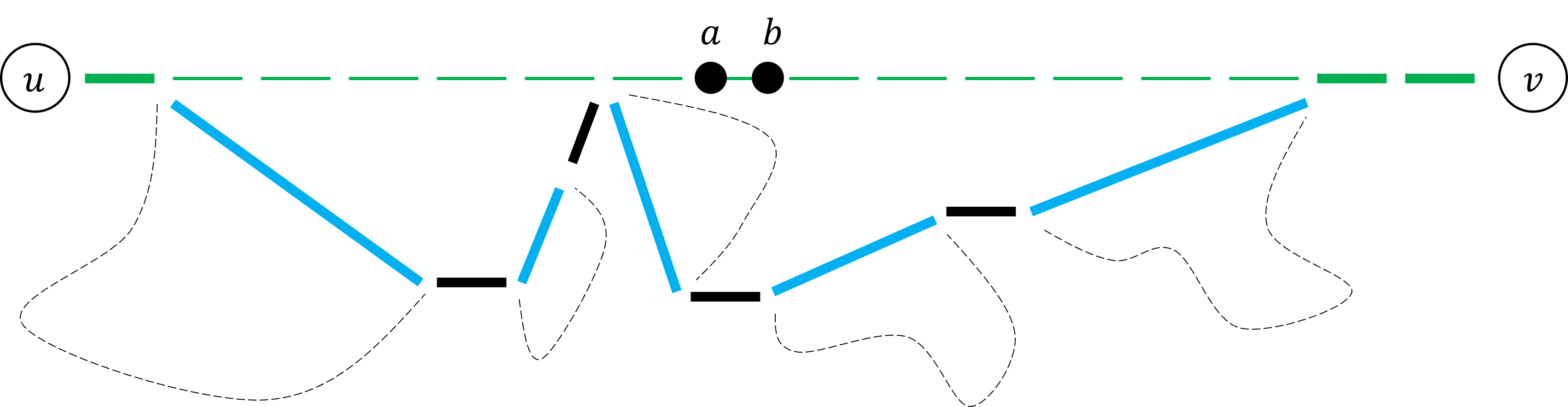
Figure 1: $P_{u,v}$ is marked by green edges. Every edge of the hopset $H$ is colored in blue, and the shortest path of $G$ connecting its ends is marked by a dashed line. The edges of the path $P\subseteq G\cup H$ are marked by a thick line, and we assume by negation that its detours are disjoint from $P_{u,v}$. Then, since also $P$ doesn’t use the edge $(a,b)$ of $P_{u,v}$, there must be a simple cycle with size $\leq|P_{u,v}|+|\hat{P}|$.

For (2), given $(x,y)\in H$ such that $w(x,y)\leq\alpha\delta$, we need to bound the number of pairs $u,v\in V$ such that $d(u,v)=\delta$ and $P_{u,v}\cap P_{x,y}\neq\emptyset$. Let $(a,b)\in P_{x,y}$. Every path of length $\delta$ that passes through $(a,b)$ is a concatenation of a path of length $i$ that ends in $a$, the edge $(a,b)$ and a path of length $\delta-1-i$ from $b$, for some $i\in[0,\delta-1]$. Fixing $i$, we can look at the BFS trees $T_{a},T_{b}$ of $a,b$ respectively, up to the $i$’th and $(\delta-1-i)$’th level respectively. Since the degree of any vertex in $G$ is $p+1$, $T_{a}$ contains at most $p^{i}$ leaves, and $T_{b}$ contains at most $p^{\delta-1-i}$ leaves. Therefore, the number of concatenations of paths as above is bounded by:

$$\sum_{i=0}^{\delta-1}p^{i}\cdot p^{\delta-1-i}=\sum_{i=0}^{\delta-1}p^{\delta-1}=\delta p^{\delta-1}\leavevmode\nobreak\ .$$

Since $P_{x,y}$ contains at most $\alpha\delta$ edges, we get that the number of paths $P_{u,v}$ such that $P_{u,v}\cap P_{x,y}\neq\emptyset$ and $|P_{u,v}|=\delta$, is bounded by $\alpha\delta\cdot\delta p^{\delta-1}=\alpha\delta^{2}p^{\delta-1}$.

Finally, using the two properties of the bipartite graph, we count its edges:

$$\frac{1}{2}np^{\delta}\stackrel{{\scriptstyle\text{lemma \ref{lemma:ManyPaths}}}}{{\leq}}|Q_{\delta}|=|A|\stackrel{{\scriptstyle\text{(1)}}}{{\leq}}\sum_{P\in A}deg_{\hat{E}}(P)=|\hat{E}|=\sum_{e\in B}deg_{\hat{E}}(e)\stackrel{{\scriptstyle\text{(2)}}}{{\leq}}|B|\alpha\delta^{2}p^{\delta-1}\leq|H|\alpha\delta^{2}p^{\delta-1}\leavevmode\nobreak\ .$$

Rearranging this inequality, we get

$$|H|\geq\frac{1}{2\alpha\delta^{2}}np=\frac{D}{2\alpha\delta^{2}}n\cdot n^{\frac{1}{\gamma}}=\frac{D}{2\alpha\delta^{2}}n^{1+\frac{1}{\gamma}}\leavevmode\nobreak\ .$$

Recall that $|H|\leq Cn^{1+\frac{1}{k}}$, so when choosing large enough $n$, it must be that $k\leq\gamma$.

Summarizing our proof so far, we showed that for fixed $\gamma\geq 1$, $\alpha>0$ and a constant $C$, there is a graph $G$ such that every $(\alpha,\beta)$-hopset $H$ for $G$, with size $\leq Cn^{1+\frac{1}{k}}$, either satisfies $\beta\geq\delta$, or satisfies $k\leq\gamma$.

Choose $\gamma=k-1$. Now the matching graph $G$ has the property that every $(\alpha,\beta)$-hopset $H$ for $G$, with size $\leq Cn^{1+\frac{1}{k}}$, must have $\beta\geq\delta$. By $\delta$’s definition:

$$\beta\geq\delta=\lfloor\frac{\gamma-1}{\alpha+1}\rfloor=\lfloor\frac{k-2}{\alpha+1}\rfloor\leavevmode\nobreak\ .$$

∎

3 A Unified Construction of Hopsets

Let $G=(V,E)$ be a weighted undirected graph. Our main construction depends on the choice of several parameters:

1. A positive integer $k\geq 1$.

2. A positive integer $F\geq 1$.

3. A monotone non-decreasing function $f:\mathbb{N}\rightarrow\mathbb{N}$ such that for every $0\leq i\leq F$, $i\leq f(i)\leq F$.

4. A sequence of non-negative numbers $\{\lambda_{j}\}_{j=0}^{F-1}$.

The resulting construction is a hopset $H(k,f,\{\lambda_{j}\},F)$. In the definition below, notice that this construction is actually not deterministic, but is created using some random choices.

The construction starts by creating a non-increasing sequence of sets $V=A_{0}\supseteq A_{1}\supseteq...\supseteq A_{F}$. The set $A_{j+1}$ is defined by selecting each vertex from $A_{j}$ independently with probability $n^{-\frac{\lambda_{j}}{k}}$ (recall that $n=|V|$).

Given this sequence, define some useful notations:

1. For a vertex $u\in V$, denote by $i(u)$ the level of $u$, which is the only $i$ such that $u\in A_{i}\setminus A_{i+1}$ (for this definition $A_{F+1}=\emptyset$).

2. The $j$’th pivot of $u$, $p_{j}(u)$, is the vertex of $A_{j}$ which is the closest to $u$.

3. The $j$’th bunch of $u$ is the set $B_{j}(u)=\{v\in A_{j}\;|\;d(u,v)<d(u,p_{j+1}(u))\}$.
   (Whenever $A_{j+1}=\emptyset$ or $A_{j+1}$ is undefined, then also $p_{j+1}(u)$ is undefined, and we say that $d(u,p_{j+1}(u))=\infty$, so $B_{j}(u)=A_{j}$).

Definition 1.

$$H(k,f,\{\lambda_{j}\},F)=\bigcup_{u\in V}\bigcup_{j=0}^{F-1}\{(u,p_{j}(u))\}\cup\bigcup_{u\in V}\bigcup_{j=i(u)}^{f(i(u))}\{(u,v)\;|\;v\in B_{j}(u)\}.$$

In words, $H(k,f,\{\lambda_{j}\},F)$ consists of all the edges of the form $(u,p_{j}(u))$, for every $u$ and $j$, and of all the edges $(u,v)$ such that $v\in B_{j}(u)$ for some $j\in[i(u),f(i(u))]$.

For clarity, we briefly summarize the role of each parameter in $H(k,f,\{\lambda_{j}\},F)$:

1. $k$ controls the size of the hopset, which (under certain conditions) is expected to be $O(F^{2}\cdot n^{1+\frac{1}{k}})$.

2. The function $f$ determines, for each $u\in V$, the highest index of a bunch $B_{j}(u)$, such that edges of the form $(u,v)$, where $v\in B_{j}(u)$, are added to the hopset. Notice that for $j<i(u)$, $B_{j}(u)=\emptyset$, since in this case $p_{j+1}(u)=u$. Therefore, the relevant range of indexes for $u$ is $[i(u),f(i(u))]$, and this is the reason $f$ has to satisfy $f(i)\geq i$ for every $i$.

3. The sequence $\{\lambda_{j}\}$ controls the sampling probabilities for the sets $\{A_{j}\}$: The probability of some $u\in A_{j}$ to be in $A_{j+1}$ is $n^{-\frac{\lambda_{j}}{k}}$.

4. $F$ is the index of the last set in the sequence $\{A_{j}\}$, and we will later see that we can assume that $A_{F}=\emptyset$.

Throughout this paper, we use the following notation:

$$f^{-1}(j)=\min\{i\;|\;j\leq f(i)\}.$$

The following lemma bounds the expected size of our hopset, given certain conditions on the parameters.

Lemma 3.

Suppose that the parameters $k,f,\{\lambda_{j}\},F$ satisfy

1. $\sum_{j<F}\lambda_{j}\geq k+1$

2. $\forall_{j}\;\lambda_{j}\leq 1+\sum_{l<f^{-1}(j)}\lambda_{l}$

Then, ${\mathbb{E}}[|H(k,f,\{\lambda_{j}\},F)|]=O(F^{2}n^{1+\frac{1}{k}})$.

Proof.

Considering how $A_{i}$ is defined, we can calculate its expected size:

$${\mathbb{E}}[|A_{i}|]=n\prod_{j<i}n^{-\frac{\lambda_{j}}{k}}=n^{1-\frac{1}{k}\sum_{j<i}\lambda_{j}}.$$

Particularly, for $i=F$, ${\mathbb{E}}[|A_{F}|]=n^{1-\frac{1}{k}\sum_{j<F}\lambda_{j}}$. If we want to have $A_{F}=\emptyset$ with high probability, we can choose $F$ such that $\sum_{j<F}\lambda_{j}\geq k+1$, and therefore ${\mathbb{E}}[|A_{F}|]\leq n^{-\frac{1}{k}}$. Then, by Markov inequality, $Pr[A_{F}\neq\emptyset]=Pr[|A_{F}|\geq 1]\leq n^{-\frac{1}{k}}$, i.e. $A_{F}=\emptyset$ with high probability.

Now, fix some $u\in V$ and $j\geq i(u)$. We show that the expected size of $B_{j}(u)$ is $n^{\frac{\lambda_{j}}{k}}-1$. Let $u_{1},u_{2},u_{3},...$ be all of the vertices of $A_{j}$, ordered by their distance from $u$. If $u_{l}$ is the first vertex in this list such that $u_{l}\in A_{j+1}$, then $B_{j}(u)=\{u_{1},u_{2},...,u_{l-1}\}$, since these are exactly the vertices of $A_{j}$ that are closer to $u$ than $p_{j+1}(u)$. Notice that $l$ is a geometric random variable, since each of the $u_{i}$’s is sampled into $A_{j+1}$ independently with probability $n^{-\frac{\lambda_{j}}{k}}$, and $u_{l}$ is the first vertex that was sampled. Therefore, ${\mathbb{E}}[|B_{j}(u)|]={\mathbb{E}}[l-1]=n^{\frac{\lambda_{j}}{k}}-1$.

So, we get that in expectation:

$$|H(k,f,\{\lambda_{j}\},F)| \leq |\bigcup_{u\in V}\bigcup_{j=0}^{F-1}\{(u,p_{j}(u))\}|+|\bigcup_{u\in V}\bigcup_{j=i(u)}^{f(i(u))}\{(u,v)\;|\;v\in B_{j}(u)\}|$$

$$\leq nF+\sum_{u\in V}\sum_{j=i(u)}^{f(i(u))}n^{\frac{\lambda_{j}}{k}}$$

$$= nF+\sum_{i=0}^{F-1}|A_{i}\setminus A_{i+1}|\sum_{j=i}^{f(i)}n^{\frac{\lambda_{j}}{k}}\leavevmode\nobreak\ .$$

Recall that ${\mathbb{E}}[|A_{i}|]=n^{1-\frac{1}{k}\sum_{l<i}\lambda_{l}}$, so in expectation:

$$|H(k,f,\{\lambda_{j}\},F)|<nF+\sum_{i=0}^{F-1}n^{1-\frac{1}{k}\sum_{l<i}\lambda_{l}}\sum_{j=i}^{f(i)}n^{\frac{\lambda_{j}}{k}}=nF+\sum_{i=0}^{F-1}\sum_{j=i}^{f(i)}n^{1+\frac{1}{k}(\lambda_{j}-\sum_{l<i}\lambda_{l})}.$$

We want the expected size of $H(k,f,\{\lambda_{j}\},F)$ to be $O(F^{2}n^{1+\frac{1}{k}})$, so we choose $\{\lambda_{j}\}$ such that $\forall_{i}\forall_{j\in[i,f(i)]}\;\lambda_{j}\leq 1+\sum_{l<i}\lambda_{l}$, and then we get

$$\sum_{i=0}^{F-1}\sum_{j=i}^{f(i)}n^{1+\frac{1}{k}(\lambda_{j}-\sum_{l<i}\lambda_{l})} \leq \sum_{i=0}^{F-1}\sum_{j=i}^{f(i)}n^{1+\frac{1}{k}}\leq F\max_{i}(f(i)-i+1)n^{1+\frac{1}{k}}$$ (1)

$$\leq F^{2}n^{1+\frac{1}{k}}\leavevmode\nobreak\ .$$ (2)

For this constraint on the sequence $\{\lambda_{j}\}$, for every $j$ it’s enough to take the minimal possible $i$ such that $j\in[i,f(i)]$, which is exactly $f^{-1}(j)$:

$$\forall_{j}\;\lambda_{j}\leq 1+\sum_{l<f^{-1}(j)}\lambda_{l}\leavevmode\nobreak\ .$$

∎

Given $k,f$, it makes sense to choose the largest $\{\lambda_{j}\}$ and the smallest $F$ that satisfy the constraints of lemma 3. As we will soon see in Theorem 3 below, a larger $F$ will increase the hopbound and size of our hopset. Thus, considering the constraint on $F$, we see that choosing the largest possible $\lambda_{j}$’s will be the most beneficial.

Definition 2.

Given an integer $k\geq 1$ and a non-decreasing function $f:\mathbb{N}\rightarrow\mathbb{N}$ such that $\forall_{i}\;f(i)\geq i$, the General Hopset $H(k,f)$, is the hopset $H(k,f,\{\lambda_{j}\},F)$, where $\{\lambda_{j}\}$ and F are defined by.

1. $\lambda_{j}=1+\sum_{l<f^{-1}(j)}\lambda_{l}$.

2. $F=\min\{F^{\prime}\;|\;\sum_{l<F^{\prime}}\lambda_{l}\geq k+1\}$.

3.1 Examples

3.1.1 Linear TZ

When choosing $f(j)=k$ for all $j\leq k$, and choosing $F$ and $\{\lambda_{j}\}$ according to the definition of $H(k,f)$, we get $\lambda_{j}=1$ for all $j$ (since $f^{-1}(j)=0$ for all $j\leq k$), and $k+1=\sum_{j<F}\lambda_{j}=F$.

That means, there’s a sequence $V=A_{0}\supseteq A_{1}\supseteq A_{2}\supseteq...\supseteq A_{k+1}=\emptyset$, where $A_{i+1}$ is sampled from $A_{i}$ with probability $n^{-\frac{1}{k}}$, and the size of the resulting hopset is $O(k^{2}\cdot n^{1+1/k})$. This is the same construction as shown in [TZ01], except that the distance oracle’s size there was $O(kn^{1+\frac{1}{k}})$. To match that, we use a more careful analysis, specific to this case:

Recall that ${\mathbb{E}}[|A_{i}|]=n^{1-\frac{1}{k}\sum{l<i}\lambda_{l}}=n^{1-\frac{i}{k}}$. Therefore, in expectation:

$$|H(k,f)| \leq nF+\sum_{i=0}^{F-1}|A_{i}\setminus A_{i+1}|\sum_{j=i}^{f(i)}n^{\frac{\lambda_{j}}{k}}$$

$$\leq n(k+1)+\sum_{i=0}^{k}(|A_{i}|-|A_{i+1}|)\sum_{j=i}^{k}n^{\frac{1}{k}}$$

$$\leq n(k+1)+\sum_{i=0}^{k}(n^{1-\frac{i}{k}}-n^{1-\frac{i+1}{k}})kn^{\frac{1}{k}}$$

$$= n(k+1)+k(n^{1+\frac{1}{k}}-1)=O(kn^{1+\frac{1}{k}})\leavevmode\nobreak\ .$$

As observed in [BLP20], $H(k,f)$ with this function $f$ is a $(2k-1,2)$-hopset of size $O(kn^{1+\frac{1}{k}})$.

3.1.2 Exponential TZ

Choose $f(j)=j$ for every $j$, and again choose $F$ and $\{\lambda_{j}\}$ by $H(k,f)$ definition. Since $f^{-1}(j)=j$ for every $j$, we get $\lambda_{j}=1+\sum_{l<j}\lambda_{l}\;\;\Rightarrow\;\;\lambda_{j}=2^{j}$ (proof by induction). Also,

$$k+1\approx\sum_{j<F}\lambda_{j}=2^{F}-1\;\;\Rightarrow\;\;F=\lceil\log_{2}(k+2)\rceil\leavevmode\nobreak\ .$$

That means, there’s a sequence $V=A_{0}\supseteq A_{1}\supseteq...\supseteq A_{\lceil\log_{2}(k+2)\rceil}=\emptyset$, where $A_{i+1}$ is sampled from $A_{i}$ with probability $n^{-\frac{2^{i}}{k}}$, and the size of $H(k,f)$ is $O((\log_{2}k)^{2}\cdot n^{1+1/k})$. This is the same construction as shown in section 4 in [TZ06], except that the construction’s size there was $O(\log k\cdot n^{1+\frac{1}{k}})$. To match that, notice that according to inequality (1), the size of $H(k,f)$ is

$$O(F\max_{i}(f(i)-i+1)n^{1+\frac{1}{k}})=O(\log k\cdot 1\cdot n^{1+\frac{1}{k}})=O(\log k\cdot n^{1+\frac{1}{k}})\leavevmode\nobreak\ .$$

By the analysis of [HP17, EN19], the emulator from [TZ06], which is our $H(k,f)$ with the identity $f$, is actually a $(1+\epsilon,O(\frac{\log k}{\epsilon})^{\log k})$-hopset of size $O(\log k\cdot n^{1+\frac{1}{k}})$, for every $0<\epsilon<1$ simultaneously.

4 Stretch and Hopbound Analysis Method

In this section we show that our general hopset can provide the state-of-the-art results for $(\alpha,\beta)$-hopsets, for various regimes of $\alpha$. We consider three possible regimes: $\alpha=3+\epsilon$ for some $\epsilon>0$, $\alpha=O(1)$ and $\alpha=k^{\epsilon}$ for $0<\epsilon<1$.

Given a weighted undirected graph $G$, and given the parameters $k,f$, that define $H(k,f)$, we add another parameter, which is a sequence of non-negative real numbers: $\{r_{i}\}_{i=0}^{F}$. We stress that these parameters only play a part in the analysis.

The following definition of the score of a vertex is needed for the lemma that will be proved afterwards.

Definition 3.

Given the function $f$ and the sequence $\{r_{i}\}$, the Score of a vertex $u\in V$ is:

$$score(u)=\max\{i>0\;|\;d(u,p_{i}(u))>r_{i}\text{ and }\forall_{j\in[f^{-1}(i-1),i-1]}\;d(u,p_{j}(u))\leq r_{j}\},$$

where if $p_{i}(u)$ is not defined (e.g. when $i=F$ and $A_{F}=\emptyset$), we consider $d(u,p_{i}(u))$ to be $\infty$.

Remark 1.

The set in the definition of $score(u)$ is not empty, so the score of each vertex is well defined and positive. To see this, note that if $i$ is the minimal index such that $d(u,p_{i}(u))>r_{i}$, then $i>0$ (because $p_{0}(u)=u$, so $d(u,p_{0}(u))=0\leq r_{0}$), $i\leq F$ (because $d(u,p_{F}(u))=\infty>r_{F}$) and also for every $j\in[f^{-1}(i-1),i-1]$, by the minimality of $i$, $d(u,p_{j}(u))\leq r_{j}$.

Denote $H=H(k,f)$. The following lemma lets us ”jump” from some vertex $u$ to some other vertex $u^{\prime}$, using a path in $G\cup H$, where $u^{\prime}$ is at a certain distance from $u$. These paths have low hopbound and stretch, and we will use them later to connect every pair of vertices in $G$.

Lemma 4 (Jumping Lemma).

Suppose that $score(u)=i$, then for every $u^{\prime}\in V$ such that $d(u,u^{\prime})\leq\frac{r_{i}-r_{i-1}}{2}-r_{f^{-1}(i-1)}$,

$$d_{G\cup H}^{(3)}(u,u^{\prime})\leq 3d(u,u^{\prime})+2(r_{i-1}+r_{f^{-1}(i-1)}).$$

Moreover, if also $d(u,u^{\prime})\geq\frac{2}{t}(r_{i-1}+r_{f^{-1}(i-1)})$ for some $t>0$, then:

$$d_{G\cup H}^{(3)}(u,u^{\prime})\leq(t+3)d(u,u^{\prime}).$$

Proof.

Let $u\in V$ be some vertex with $score(u)=i$ and let $u^{\prime}\in V$ be some other vertex. We look at the following potential path:

$$u\rightarrow p_{f^{-1}(i-1)}(u)\rightarrow p_{i-1}(u^{\prime})\rightarrow u^{\prime}.$$

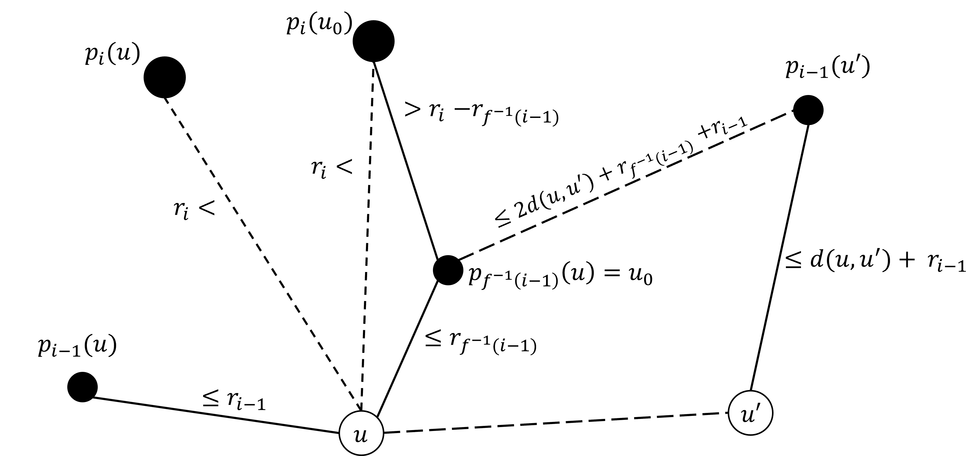
Figure 2: The potential path between $u$ and $u^{\prime}$. Notice that $d(u,p_{i-1}(u))\leq r_{i-1}$ and $d(u,p_{f^{-1}(i-1)}(u))\leq r_{f^{-1}(i-1)}$, since $score(u)=i$.

The reason we look at the $(i-1)$’th pivot of $u^{\prime}$ is that this is the highest-index pivot of $u^{\prime}$, such that we can still bound the distance to it:

$$d(u^{\prime},p_{i-1}(u^{\prime}))\leq d(u^{\prime},p_{i-1}(u))\leq d(u^{\prime},u)+d(u,p_{i-1}(u))\leq d(u^{\prime},u)+r_{i-1}\leavevmode\nobreak\ .$$ (3)

The reason we look at the $f^{-1}(i-1)$’th pivot of $u$ is that this is the lowest-index pivot of $u$ that still can be connected to $p_{i-1}(u^{\prime})$ through a $H$-edge, according to our construction.

Notice that in the path above, the first and the last arrows represent edges that do exist in $H$. We now bound the distance between $p_{f^{-1}(i-1)}(u)$ and $p_{i-1}(u^{\prime})$. Recall that $score(u)=i$, and therefore for every
$j\in[f^{-1}(i-1),i-1]$, $d(u,p_{j}(u))\leq r_{j}$. In particular:

$$d(u,p_{f^{-1}(i-1)}(u))\leq r_{f^{-1}(i-1)},$$

and now we can see that:

$$d(p_{f^{-1}(i-1)}(u),p_{i-1}(u^{\prime})) \leq d(p_{f^{-1}(i-1)}(u),u)+d(u,u^{\prime})+d(u^{\prime},p_{i-1}(u^{\prime}))$$

$$\stackrel{{\scriptstyle\eqref{eq:u'}}}{{\leq}} r_{f^{-1}(i-1)}+d(u,u^{\prime})+(d(u,u^{\prime})+r_{i-1})$$

$$= 2d(u,u^{\prime})+r_{f^{-1}(i-1)}+r_{i-1}\leavevmode\nobreak\ .$$

For convenience, we denote $u_{0}=p_{f^{-1}(i-1)}(u)$, and we also bound the distance $d(u_{0},p_{i}(u_{0}))$.

$$r_{i}<d(u,p_{i}(u))\leq d(u,p_{i}(u_{0}))\leq d(u,u_{0})+d(u_{0},p_{i}(u_{0}))\leq r_{f^{-1}(i-1)}+d(u_{0},p_{i}(u_{0}))\;\;\Rightarrow$$

$$\Rightarrow\;\;d(u_{0},p_{i}(u_{0}))>r_{i}-r_{f^{-1}(i-1)}.$$

Figure 2 summarizes all of the computations above.

Recall that the vertex $u_{0}$ is connected through an edge of $H$ to any vertex $v\in B_{j}(u_{0})$, for every $j\in[i(u_{0}),f(i(u_{0}))]$. Since $u_{0}$ is a $f^{-1}(i-1)$’th pivot, we know that $i(u_{0})\geq f^{-1}(i-1)$, so using the fact that $f$ is non-decreasing:

$$i-1\leq f(f^{-1}(i-1))\leq f(i(u_{0})).$$

Also, since $d(u_{0},p_{i}(u_{0}))>r_{i}-r_{f^{-1}(i-1)}>0$, it cannot be that $i(u_{0})\geq i$ (otherwise $u_{0}$ would be the $i$’th pivot of itself and the distance $d(u_{0},p_{i}(u_{0}))$ would be $0$). Then we got that $i-1\in[i(u_{0}),f(i(u_{0}))]$.

Therefore, $u_{0}$ is connected to every vertex of $B_{i-1}(u_{0})$. Since $p_{i-1}(u^{\prime})\in A_{i-1}$, a sufficient condition for $p_{i-1}(u^{\prime})$ to be in $B_{i-1}(u_{0})$, which would imply that $(u_{0},p_{i-1}(u^{\prime}))\in H$, is

$$2d(u,u^{\prime})+r_{f^{-1}(i-1)}+r_{i-1}\leq r_{i}-r_{f^{-1}(i-1)},$$

i.e.

$$d(u,u^{\prime})\leq\frac{r_{i}-r_{i-1}}{2}-r_{f^{-1}(i-1)}.$$

In case that this criteria is satisfied, $u_{0}=p_{f^{-1}(i-1)}(u)$ and $p_{i-1}(u^{\prime})$ are connected, and we get a $3$-hops path from $u$ to $u^{\prime}$. The weight of this path is:

$$d_{G\cup H}^{(3)}(u,u^{\prime}) \leq r_{f^{-1}(i-1)}+(2d(u,u^{\prime})+r_{f^{-1}(i-1)}+r_{i-1})+(d(u,u^{\prime})+r_{i-1})$$

$$= 3d(u,u^{\prime})+2(r_{i-1}+r_{f^{-1}(i-1)})\leavevmode\nobreak\ .$$

Let $t>0$ be some real number. If it happens to be that the above $u,u^{\prime}$ satisfy also $r_{i-1}+r_{f^{-1}(i-1)}\leq\frac{t}{2}d(u,u^{\prime})$ (or equivalently $d(u,u^{\prime})\geq\frac{2}{t}(r_{i-1}+r_{f^{-1}(i-1)})$), then we get a $3$-hops path between them, of weight $\leq 3d(u,u^{\prime})+td(u,u^{\prime})=(t+3)d(u,u^{\prime})$, i.e. a stretch of $t+3$. ∎

Lemma 4 implies that if we want to have many pairs of vertices, such that there’s a $3$-hops path between them, with stretch $\approx t$, it’s better to choose the parameters $\{r_{i}\}$ such that $\frac{2}{t}(r_{i-1}+r_{f^{-1}(i-1)})\leq\frac{r_{i}-r_{i-1}}{2}-r_{f^{-1}(i-1)}$, i.e.

$$r_{i}\geq(1+\frac{4}{t})r_{i-1}+(2+\frac{4}{t})r_{f^{-1}(i-1)}$$ (4)

From now on, we indeed assume that the $\{r_{i}\}$ we chose satisfy this inequality.

Let $u,v\in V$ be a pair of vertices, and let $u=u_{0},u_{1},u_{2},...,u_{d}=v$ be the shortest path between them. We want to use the ”jumps” that lemma 4 provides, in order to find a low hopbound path in $G\cup H$ between $u,v$.

Lemma 5.

Suppose that $score(u_{j})=i$ and let

$$l=\max\{l^{\prime}\geq j\;|\;d(u_{j},u_{l^{\prime}})\leq\frac{r_{i}-r_{i-1}}{2}-r_{f^{-1}(i-1)}\}.$$

Then if $l<d$, we have:

1. $d_{G\cup H}^{(4)}(u_{j},u_{l+1})\leq(t+3)d(u_{j},u_{l+1})$

2. $d(u_{j},u_{l+1})\geq\frac{4}{t}r_{f^{-1}(i-1)}$

Proof.

Denote by $W$ the weight of the edge $(u_{l},u_{l+1})$. We look at two different cases.

Case 1: $d(u_{j},u_{l})\geq\frac{2}{t}(r_{i-1}+r_{f^{-1}(i-1)})$. In this case, by lemma 4:

$$d_{G\cup H}^{(4)}(u_{j},u_{l+1})\leq d_{G\cup H}^{(3)}(u_{j},u_{l})+W\leq(t+3)d(u_{j},u_{l})+W<(t+3)(d(u_{j},u_{l})+W)=(t+3)d(u_{j},u_{l+1}).$$

Case 2: $d(u_{j},u_{l})<\frac{2}{t}(r_{i-1}+r_{f^{-1}(i-1)})$. By lemma 4, we have that $d_{G\cup H}^{(3)}(u_{j},u_{l})\leq 3d(u_{j},u_{l})+2(r_{i-1}+r_{f^{-1}(i-1)})$. Also, recall that we assumed that inequality (4) holds, which is equivalent to the fact that $\frac{r_{i}-r_{i-1}}{2}-r_{f^{-1}(i-1)}\geq\frac{2}{t}(r_{i-1}+r_{f^{-1}(i-1)})$. Therefore,

$$d(u_{j},u_{l+1})>\frac{r_{i}-r_{i-1}}{2}-r_{f^{-1}(i-1)}\geq\frac{2}{t}(r_{i-1}+r_{f^{-1}(i-1)})\leavevmode\nobreak\ .$$

We get that

$$2(r_{i-1}+r_{f^{-1}(i-1)})\leq td(u_{j},u_{l+1})=t(d(u_{j},u_{l})+W),$$

and we finally have,

$$d_{G\cup H}^{(4)}(u_{j},u_{l+1}) \leq d_{G\cup H}^{(3)}(u_{j},u_{l})+W$$

$$\leq 3d(u_{j},u_{l})+2(r_{i-1}+r_{f^{-1}(i-1)})+W$$

$$\leq 3d(u_{j},u_{l})+t(d(u_{j},u_{l})+W)+W$$

$$= (t+3)d(u_{j},u_{l})+(t+1)W$$

$$< (t+3)d(u_{j},u_{l+1})\leavevmode\nobreak\ .$$

In both cases, we saw that $d(u_{j},u_{l+1})\geq\frac{2}{t}(r_{i-1}+r_{f^{-1}(i-1)})$, and since $\{r_{i}\}$ is a non-decreasing sequence (can be seen by inequality (4)), we get:

$$d(u_{j},u_{l+1})\geq\frac{2}{t}(r_{i-1}+r_{f^{-1}(i-1)})\geq\frac{4}{t}r_{f^{-1}(i-1)}\leavevmode\nobreak\ .$$

∎

The following theorem presents the size, the stretch and the hopbound for our hopset, $H(k,f)$. It uses lemma 5 repeatedly between every pair of vertices $u,v\in V$.

Theorem 3.

Given an integer $k$, a monotone non-decreasing function $f:\mathbb{N}\rightarrow\mathbb{N}$ such that $\forall_{i}f(i)\geq i$, parameters $\{\lambda_{j}\}$ such that $\forall_{j}\lambda_{j}\leq 1+\sum_{l<f^{-1}(j)}\lambda_{l}$ and $F$ such that $\sum_{j<F}\lambda_{j}\geq k+1$, we can build a hopset for an undirected weighted graph $G$, with the following properties, simultaneously for every $t>0$:

1. Size $O(F^{2}n^{1+1/k})$.

2. Stretch $2t+3$.

3. Hopbound $O(r_{F})$,
   where $\{r_{i}\}$ satisfies $r_{0}=1$ and $\forall_{i>0}\;r_{i}\geq(1+\frac{4}{t})r_{i-1}+(2+\frac{4}{t})r_{f^{-1}(i-1)}$.

Proof.

Given $G,k,f$, build $H(k,f)$ on $G$. By lemma 3, this hopset has the wanted size. Let $u,v\in V$ be a pair of vertices, and let $u=u_{0},u_{1},u_{2},...,u_{d}=v$ be the shortest path between them. We use lemma 5 to find a path between $u$ and $v$. Starting with $j=0$, find $l=\max\{l^{\prime}\geq j\;|\;d(u_{j},u_{l^{\prime}})\leq\frac{r_{i}-r_{i-1}}{2}-r_{f^{-1}(i-1)}\}$, where $score(u_{j})=i$. If $l=d$, stop the process and denote $v^{\prime}=u_{j}$. Otherwise, set $j\leftarrow l+1$, and continue in the same way.

This process creates a subsequence of $u_{0},...,u_{d}$: $u=v_{0},v_{1},v_{2},...,v_{b}=v^{\prime}$, such that for every $j<b$ we have $d_{G\cup H}^{(4)}(v_{j},v_{j+1})\leq(t+3)d(v_{j},v_{j+1})$ (by lemma 5). For $v^{\prime}=v_{b}$ we have $d(v^{\prime},v)\leq\frac{r_{i}-r_{i-1}}{2}-r_{f^{-1}(i-1)}$, where $score(v^{\prime})=i$. For this last segment, we get from lemma 4 that

$$d_{G\cup H}^{(3)}(v^{\prime},v)\leq 3d(v^{\prime},v)+2(r_{i-1}+r_{f^{-1}(i-1)})\leq 3d(v^{\prime},v)+4r_{F}$$

(again, by inequality (4), $\{r_{i}\}$ is a non-decreasing sequence).

When summing over the entire path, we get:

$$d_{G\cup H}^{(4b+3)}(u,v) \leq \sum_{j=0}^{b-1}(t+3)d(v_{j},v_{j+1})+3d(v^{\prime},v)+4r_{F}$$

$$= (t+3)d(u,v^{\prime})+3d(v^{\prime},v)+4r_{F}$$

$$\leq (t+3)d(u,v)+4r_{F}\leavevmode\nobreak\ .$$

To bound $b$, we notice that by lemma 5, for every $j<b$:

$$d(v_{j},v_{j+1})\geq\frac{4}{t}r_{f^{-1}(i-1)}\geq\frac{4}{t}r_{0}\leavevmode\nobreak\ .$$

So, the number of these ”jumps” couldn’t be greater than $\frac{d(u,v)}{\frac{4}{t}r_{0}}=\frac{t\cdot d(u,v)}{4r_{0}}$, and we finally got:

$$d_{G\cup H}^{(\frac{t\cdot d(u,v)}{r_{0}}+3)}(u,v)\leq(t+3)d(u,v)+4r_{F}\leavevmode\nobreak\ ,$$

and this is true for every sequence $\{r_{i}\}$ that satisfies $\forall_{i>0}\;r_{i}\geq(1+\frac{4}{t})r_{i-1}+(2+\frac{4}{t})r_{f^{-1}(i-1)}$ (even if it doesn’t satisfy $r_{0}=1$).

Given such sequence $\{r_{i}\}$, we can define a new sequence as follows:

$$r^{\prime}_{i}=\frac{t\cdot d(u,v)\cdot r_{i}}{4r_{F}}\leavevmode\nobreak\ .$$

The new sequence clearly still satisfies the same inequality, so if we use it instead of $\{r_{i}\}$, we get that for our specific $u,v$:

$$d_{G\cup H}^{(\frac{t\cdot d(u,v)}{r^{\prime}_{0}}+3)}(u,v)\leq(t+3)d(u,v)+4r^{\prime}_{F}\;\;\;\;\Rightarrow$$

$$\Rightarrow\;\;\;\;d_{G\cup H}^{(4r_{F}+3)}(u,v)\leq(t+3)d(u,v)+t\cdot d(u,v)=(2t+3)d(u,v)\leavevmode\nobreak\ ,$$

i.e. the stretch of this new path is $2t+3$, and its hopbound is $4r_{F}+3$.

Although we chose $\{r^{\prime}_{i}\}$ for a specific pair of vertices, this choice of $\{r^{\prime}_{i}\}$ doesn’t change our construction at all, but only the analysis. So, we proved that for each $u,v\in V$, there is a path between them in $G\cup H$, with stretch $2t+3$ and hopbound $4r_{F}+3$, for our initial choice of $\{r_{i}\}$. ∎

4.1 Applications

4.1.1 $(3+\epsilon)$-stretch

In theorem 3, choose the function $f(i)=i$, and choose $\{\lambda_{j}\}$ and $F$ according to definition 2 of $H(k,f)$. Then, $\lambda_{j}=2^{j}$ (proof by induction), and $F=\lceil\log_{2}(k+2)\rceil$. For any $t>0$, it’s best to choose $\{r_{i}\}$ as small as possible, while still satisfying inequality (4), i.e. to choose $\{r_{i}\}$ such that $r_{0}=1$ and

$$r_{i}=(1+\frac{4}{t})r_{i-1}+(2+\frac{4}{t})r_{f^{-1}(i-1)}=(3+\frac{8}{t})r_{i-1}\leavevmode\nobreak\ ,$$

so $r_{i}=(3+\frac{8}{t})^{i}$. By our analysis, we get that our construction (which is the same construction as in section 4 in [TZ06]), is a hopset with stretch $2t+3$, hopbound $O((3+\frac{8}{t})^{\lceil\log_{2}(k+2)\rceil})=O(k^{\log_{2}(3+\frac{8}{t})})$ and size $O(\log k\cdot n^{1+\frac{1}{k}})$ (see subsection 3.1.2). Denoting $\epsilon=2t$, we get a hopset with:

1. Stretch $3+\epsilon$.

2. Hopbound $O(k^{\log_{2}(3+\frac{16}{\epsilon})})$.

3. Size $O(\log k\cdot n^{1+\frac{1}{k}})$.

This hopset improves the results of [EGN19, BLP20] for hopsets with stretch $3+\epsilon$. Compared to [BLP20] it has no $\log\Lambda$-factor in the size of the hopset (a $\log k$ replaces it), and in addition, this hopset has the mentioned properties simultaneously for all $\epsilon>0$. Also, our hopset has superior hopbound compared to [EGN19], there it was at least $k^{2}$.

4.1.2 Constant Stretch $O(c)$

Given some integer $c$, choose in theorem 3 the following function:

$$f(i)=\lfloor\frac{i}{c}\rfloor\cdot c+c-1\leavevmode\nobreak\ .$$

This function rounds $i$ to the largest multiplication of $c$ that is not larger than $i$, and then adds $c-1$. In this case,

$$f^{-1}(i)=\lfloor\frac{i}{c}\rfloor\cdot c\leavevmode\nobreak\ ,$$

so in $H(k,f)$’s definition, we get $\lambda_{i}=1+\sum_{l<\lfloor\frac{i}{c}\rfloor\cdot c}\lambda_{l}$. From this equation, it is easy to notice that $\forall_{i}\forall_{j\in[0,c-1]}\lambda_{ic+j}=\lambda_{ic}$, so we have:

$$\lambda_{ic}=1+\sum_{l<\lfloor\frac{ic}{c}\rfloor\cdot c}\lambda_{l}=1+\sum_{l<ic}\lambda_{l}=1+\sum_{l<i}c\lambda_{lc},$$

therefore,

$$\lambda_{ic}=1+\sum_{l<i}c\lambda_{lc}=1+\sum_{l<i-1}c\lambda_{lc}+c\lambda_{(i-1)c}=\lambda_{(i-1)c}+c\lambda_{(i-1)c}=(c+1)\lambda_{(i-1)c}\leavevmode\nobreak\ .$$

so $\lambda_{ic+j}=\lambda_{ic}=(c+1)^{i}$ for all $j\in[0,c-1]$.

For choosing $\{r_{i}\}$, we again try to minimize it, and we get the following equation:

$$r_{i}=(1+\frac{4}{t})r_{i-1}+(2+\frac{4}{t})r_{\lfloor\frac{i-1}{c}\rfloor\cdot c}\leavevmode\nobreak\ .$$

We take some index of the form $ic+j$, when $j\in[0,c-1]$. Then,

$$r_{ic+j+1}=(1+\frac{4}{t})r_{ic+j}+(2+\frac{4}{t})r_{ic}\leavevmode\nobreak\ .$$ (5)

We prove by induction that for every $j\in[0,c-1]$,

$$r_{ic+j}=[(1+\frac{4}{t})^{j}(\frac{t}{2}+2)-(\frac{t}{2}+1)]r_{ic}\leavevmode\nobreak\ .$$

1. For $j=0$, $[(1+\frac{4}{t})^{0}(\frac{t}{2}+2)-(\frac{t}{2}+1)]r_{ic}=r_{ic}$.

2. For $j>0$,

   $$r_{ic+j} = (1+\frac{4}{t})r_{ic+j-1}+(2+\frac{4}{t})r_{ic}$$

   $$= [(1+\frac{4}{t})(1+\frac{4}{t})^{j-1}(\frac{t}{2}+2)-(1+\frac{4}{t})(\frac{t}{2}+1)]r_{ic}+(2+\frac{4}{t})r_{ic}$$

   $$= [(1+\frac{4}{t})^{j}(\frac{t}{2}+2)-(\frac{t}{2}+1+2+\frac{4}{t})+(2+\frac{4}{t})]r_{ic}$$

   $$= [(1+\frac{4}{t})^{j}(\frac{t}{2}+2)-(\frac{t}{2}+1)]r_{ic}\leavevmode\nobreak\ .$$

Also, notice that when setting $j=c-1$ in (5), we get

$$r_{(i+1)c} = (1+\frac{4}{t})r_{ic+c-1}+(2+\frac{4}{t})r_{ic}$$

$$= (1+\frac{4}{t})[(1+\frac{4}{t})^{c-1}(\frac{t}{2}+2)-(\frac{t}{2}+1)]r_{ic}+(2+\frac{4}{t})r_{ic}$$

$$= [(1+\frac{4}{t})^{c}(\frac{t}{2}+2)-(\frac{t}{2}+1)]r_{ic}\leavevmode\nobreak\ ,$$

and therefore $r_{ic}=[(1+\frac{4}{t})^{c}(\frac{t}{2}+2)-(\frac{t}{2}+1)]^{i}$. We can choose now $t=4c$, and then we get that

$$r_{ic}=[(1+\frac{1}{c})^{c}(2c+2)-(2c+1)]^{i}\leavevmode\nobreak\ .$$

Recall that $F$ is the minimal such that $\sum_{l<F}\lambda_{l}\geq k+1$. We prove in appendix A that:

$$r_{F}\leq 96e^{2}k^{1+\frac{2}{\ln c}}\leavevmode\nobreak\ .$$

We finally get that our hopset has:

1. Stretch $8c+3$.

2. Hopbound $O(k^{1+\frac{2}{\ln c}})$.

3. Size $O(c\log_{c}k\cdot n^{1+\frac{1}{k}})$.

where the size expression is due to inequality (1):

$$|H(k,f)|\leq F\max_{i}(f(i)-i+1)n^{1+\frac{1}{k}}=F\cdot c\cdot n^{1+\frac{1}{k}}$$

This result improves the state-of-the-art result described in table 1 for hopsets with a constant stretch $O(c)$, by removing the $\log\Lambda$-factor from the size.

4.1.3 $O(k^{\epsilon})$-stretch

For getting a stretch of $O(k^{\epsilon})$, we use a more involved analysis than just using theorem 3. For a fixed integer $c$ that will be chosen later, we use the same function $f$ as in the previous subsection:

$$f(i)=\lfloor\frac{i}{c}\rfloor\cdot c+c-1\leavevmode\nobreak\ .$$

By the computations in the previous subsection, we know that:

1. $f^{-1}(i)=\lfloor\frac{i}{c}\rfloor\cdot c$.

2. $\lambda_{ic+j}=(c+1)^{i}$.

3. Given $t>0$, if $\{r_{i}\}$ satisfies $\forall_{i>0}\;r_{i}\geq(1+\frac{4}{t})r_{i-1}+(2+\frac{4}{t})r_{f^{-1}(i-1)}$ , then:

   $$r_{ic+j}=[(1+\frac{4}{t})^{j}(\frac{t}{2}+2)-(\frac{t}{2}+1)]r_{ic}\leavevmode\nobreak\ ,$$

   $$r_{ic}=[(1+\frac{4}{t})^{c}(\frac{t}{2}+2)-(\frac{t}{2}+1)]^{i}r_{0}\leavevmode\nobreak\ .$$

Here, we choose $t=4c$, so we get:

$$r_{ic+j}=[(1+\frac{1}{c})^{j}(2c+2)-(2c+1)]r_{ic}\leavevmode\nobreak\ ,$$

$$r_{ic}=[(1+\frac{1}{c})^{c}(2c+2)-(2c+1)]^{i}r_{0}\leavevmode\nobreak\ .$$

In particular:

$$r_{c}=[(1+\frac{1}{c})^{c}(2c+2)-(2c+1)]r_{0}\geq[2(2c+2)-(2c+1)]r_{0}>cr_{0}\leavevmode\nobreak\ .$$

According to $H(k,f)$’s definition, $F$ is the minimal $F$ such that $\sum_{l<F}\lambda_{l}\geq k+1$. In appendix A we estimate $r_{F}$ for this $F$, and we get that:

$$r_{F}\leq 96e^{2}k^{1+\frac{2}{\ln c}}\cdot r_{0}\leavevmode\nobreak\ .$$

Let $u,v\in V$ be a pair of vertices, and let $u=u_{0},u_{1},u_{2},...,u_{d}=v$ be the shortest path between them. Similarly to the proof of theorem 3, we use lemma 5 to find a path between $u$ and $v$, with a single difference: When ”standing” on a vertex $u_{j}$ with $score(u_{j})\leq c$, we don’t use the Jumping Lemma.

Lemma 6.

Denote $H=H(k,f)$. Then,

$$d_{G\cup H}^{(\frac{4c\cdot d(u,v)}{r_{c}}+3)}(u,v)\leq(4c+3)d(u,v)+r_{F}\leavevmode\nobreak\ .$$

For proving this lemma, we use two useful facts:

Fact 4.

For every $x\in V$, either $score(x)>c$, or $d(x,p_{c}(x))>r_{c}$.

For proving this fact, let $i$ be the minimal index that is greater or equal to $c$ and $d(x,p_{i}(x))>r_{i}$. If $i=c$, we’re done. Otherwise, notice that $f^{-1}(i-1)\geq c$, so for all $j\in[f^{-1}(i-1),i-1]$ we have $d(x,p_{j}(x))\leq r_{j}$, i.e. $score(x)=i>c$.

Fact 5.

For $x,y\in V$ such that $d(x,p_{c}(x))>c\cdot d(x,y)$,

$$d_{G\cup H}^{(2)}(x,y)\leq(2c+1)\cdot d(x,y)\leavevmode\nobreak\ .$$

Proof.

Let $i^{*}$ be the minimal index such that $p_{i^{*}}(x)\in B_{i^{*}}(y)$ or $p_{i^{*}}(y)\in B_{i^{*}}(x)$. We can prove by induction that for every $j\leq\min\{i^{*},c\}$,

$$d(x,p_{j}(x))\leq j\cdot d(x,y)\leavevmode\nobreak\ \leavevmode\nobreak\ \leavevmode\nobreak\ \textrm{and}\leavevmode\nobreak\ \leavevmode\nobreak\ \leavevmode\nobreak\ d(y,p_{j}(y))\leq j\cdot d(x,y).$$

For $j=0$, this is trivial since $p_{0}(x)=x$ and $p_{0}(y)=y$. For $j>0$, we assumed inductively that both $d(x,p_{j-1}(x))\leq(j-1)d(x,y)$ and $d(y,p_{j-1}(y))\leq(j-1)d(x,y)$. The fact that $p_{j-1}(y)\notin B_{j-1}(x)$ and $j\leq c$ indicates that $d(p_{j-1}(y),x)\geq d(x,p_{j}(x))$. So,

$$d(x,p_{j}(x))\leq d(x,p_{j-1}(y))\leq d(x,y)+d(y,p_{j-1}(y))\leq d(x,y)+(j-1)d(x,y)=j\cdot d(x,y)\leavevmode\nobreak\ .$$

The proof that $d(y,p_{j}(y))\leq j\cdot d(x,y)$ is symmetric. This concludes the inductive proof.

Now, since we know that $d(x,p_{c}(x))>c\cdot d(x,y)$, it must be that $i^{*}<c$. If $p_{i^{*}}(x)\in B_{i^{*}}(y)$ then the edges $(x,p_{i^{*}}(x))$ and $(y,p_{i^{*}}(x))$ are in the hopset $H$. In this case we have,

$$d_{G\cup H}^{(2)}(x,y) \leq d(x,p_{i^{*}}(x))+d(p_{i^{*}}(x),y)$$

$$\leq d(x,p_{i^{*}}(x))+d(p_{i^{*}}(x),x)+d(x,y)$$

$$\leq i^{*}\cdot d(x,y)+i^{*}\cdot d(x,y)+d(x,y)$$

$$= (2i^{*}+1)d(x,y)$$

$$< (2c+1)d(x,y)\leavevmode\nobreak\ .$$

Otherwise, $p_{i^{*}}(y)\in B_{i^{*}}(x)$, then the edges $(x,p_{i^{*}}(y))$ and $(y,p_{i^{*}}(y))$ are in the hopset, and we get the same bound on $d_{G\cup H}^{(2)}(x,y)$.

∎

Proof of lemma 6.

Starting with $j=0$, define $l$ as follows:

1. If $score(u_{j})>c$, set $l=\max\{l^{\prime}\geq j\;|\;d(u_{j},u_{l^{\prime}})\leq\frac{r_{i}-r_{i-1}}{2}-r_{f^{-1}(i-1)}\}$.

2. Otherwise, set $l=\max\{l^{\prime}\geq j\;|\;d(u_{j},u_{l^{\prime}})\leq\frac{r_{c}}{c}\}$.

If $l=d$, stop the process and denote $v^{\prime}=u_{j}$. Otherwise, set $j\leftarrow l+1$, and continue in the same way.

This process creates a subsequence of $u_{0},...,u_{d}$: $u=v_{0},v_{1},v_{2},...,v_{b}=v^{\prime}$, such that for every $i<b$, if $score(v_{i})>c$, we have $d_{G\cup H}^{(4)}(v_{i},v_{i+1})\leq(4c+3)d(v_{i},v_{i+1})$ (by lemma 5).

For $i<b$, if $score(v_{i})>c$ doesn’t hold, then by fact 4, $d(v_{i},p_{c}(v_{i}))>r_{c}$. In that case, suppose that $v_{i}=u_{j}$, and then we know that $l$ is defined such that $d(u_{j},u_{l})\leq\frac{r_{c}}{c}$. Therefore,

$$d(u_{j},p_{c}(u_{j}))>r_{c}\geq c\cdot d(u_{j},u_{l})\leavevmode\nobreak\ ,$$

and by fact 5,

$$d_{G\cup H}^{(2)}(u_{j},u_{l})\leq(2c+1)d(u_{j},u_{l})\leavevmode\nobreak\ .$$

So we get that

$$d_{G\cup H}^{(3)}(u_{j},u_{l+1}) \leq (2c+1)d(u_{j},u_{l})+W$$

$$\leq (2c+1)(d(u_{j},u_{l})+W)$$

$$= (2c+1)d(u_{j},u_{l+1})$$

$$\leq (4c+3)d(u_{j},u_{l+1})\leavevmode\nobreak\ ,$$

where $W$ is the weight of the edge $(u_{l},u_{l+1})$.

Since $v_{i+1}$ is defined to be $u_{l+1}$, we finally have that for every $i<b$:

$$d_{G\cup H}^{(4)}(v_{i},v_{i+1})\leq(4c+3)d(v_{i},v_{i+1})$$

For $v^{\prime}=v_{b}$ we consider two cases:

Case 1: $score(v^{\prime})\leq c$.

In that case, we have $d(v^{\prime},v)\leq\frac{r_{c}}{c}$, and by fact 4, $d(v^{\prime},p_{c}(v^{\prime}))>r_{c}$. So again by fact 5:

$$d_{G\cup H}^{(2)}(v^{\prime},v)\leq(2c+1)d(v^{\prime},v)\leavevmode\nobreak\ .$$

Case 2: $score(v^{\prime})=i>c$.

In that case, we have $d(v^{\prime},v)\leq\frac{r_{i}-r_{i-1}}{2}-r_{f^{-1}(i-1)}$. From lemma 4:

$$d_{G\cup H}^{(3)}(v^{\prime},v)\leq 3d(v^{\prime},v)+2(r_{i-1}+r_{f^{-1}(i-1)})\leq 3d(v^{\prime},v)+4r_{F}\leavevmode\nobreak\ .$$

In both cases we get that

$$d_{G\cup H}^{(3)}(v^{\prime},v)\leq(2c+1)d(v^{\prime},v)+4r_{F}\leavevmode\nobreak\ .$$

When summing over the entire path, we get:

$$d_{G\cup H}^{(4b+3)}(u,v)\leq\sum_{j=0}^{b-1}(4c+3)d(v_{j},v_{j+1})+(2c+1)d(v^{\prime},v)+4r_{F}\leq(4c+3)d(u,v)+4r_{F}\leavevmode\nobreak\ .$$

To bound $b$, we notice that by lemma 5, for every $i<b$ such that $score(v_{i})=j>c$ (recall that we chose $t=4c$):

$$d(v_{i},v_{i+1})\geq\frac{4}{4c}r_{f^{-1}(j-1)}\geq\frac{1}{c}r_{f^{-1}(c)}=\frac{r_{c}}{c}\leavevmode\nobreak\ .$$

For $i<b$ such that $score(v_{i})=c$, we choose $v_{i+1}$ such that $d(v_{i},v_{i+1})\geq\frac{r_{c}}{c}$.

Finally we saw that for all $i<b$:

$$d(v_{i},v_{i+1})\geq\frac{r_{c}}{c}\leavevmode\nobreak\ .$$

That means that the number of these ”jumps” couldn’t be greater than $\frac{d(u,v)}{\frac{r_{c}}{c}}=\frac{c\cdot d(u,v)}{r_{c}}$. Substituting in $b$, we get:

$$d_{G\cup H}^{(\frac{4c\cdot d(u,v)}{r_{c}}+3)}(u,v)\leq(4c+3)d(u,v)+4r_{F}\leavevmode\nobreak\ .$$

∎

Lastly, we use our estimations for $r_{c}$ and $r_{F}$ from the beginning of this subsection. Recall that:

$$r_{c}\geq cr_{0}\leavevmode\nobreak\ ,$$

and that

$$r_{F}\leq 96e^{2}k^{1+\frac{2}{\ln c}}\cdot r_{0}\leavevmode\nobreak\ ,$$

so we get that:

$$d_{G\cup H}^{(\frac{4c\cdot d(u,v)}{cr_{0}}+3)}(u,v)\leq(4c+3)d(u,v)+384e^{2}k^{1+\frac{2}{\ln c}}\cdot r_{0}\leavevmode\nobreak\ .$$

Here, instead of $r_{0}=1$, we choose $r_{0}=\frac{c}{k}d(u,v)$ and then:

$$d_{G\cup H}^{(4\frac{k}{c}+3)}(u,v)\leq(4c+3)d(u,v)+384e^{2}ck^{\frac{3}{\ln c}}\cdot d(u,v)\leavevmode\nobreak\ .$$

Let $c=\lceil k^{\epsilon}\rceil$. Then, our hopbound is:

$$4\frac{k}{c}+3=4\frac{k}{\lceil k^{\epsilon}\rceil}+3\leq 4k^{1-\epsilon}+3=O(k^{1-\epsilon})\leavevmode\nobreak\ ,$$

and the stretch is

$$4c+3+384e^{2}ck^{\frac{2}{\ln c}} = 4\lceil k^{\epsilon}\rceil+3+384e^{2}\lceil k^{\epsilon}\rceil\cdot k^{\frac{2}{\ln\lceil k^{\epsilon}\rceil}}$$

$$\leq 4\lceil k^{\epsilon}\rceil+3+384e^{2}\lceil k^{\epsilon}\rceil\cdot k^{\frac{2}{\epsilon\ln k}}$$

$$= 4\lceil k^{\epsilon}\rceil+3+384e^{2}\lceil k^{\epsilon}\rceil\cdot e^{\frac{2}{\epsilon}}$$

$$= (4+384e^{2}\cdot e^{\frac{2}{\epsilon}})\lceil k^{\epsilon}\rceil+3$$

$$= O(e^{\frac{2}{\epsilon}}k^{\epsilon})\leavevmode\nobreak\ .$$

Summarizing our result, we got a $(O(k^{\epsilon}),O(k^{1-\epsilon}))$-hopset with size

$$O(\log^{2}_{c}k\cdot n^{1+\frac{1}{k}})=O(n^{1+\frac{1}{k}}/\epsilon^{2})\leavevmode\nobreak\ .$$

This improves the size of the state-of-the-are hopsets of [BLP20] by a $\log\Lambda$ factor, while enjoying a simpler algorithm. In addition, note that in [BLP20] the construction of a hopset with stretch $O(k^{\epsilon})$, where $0<\epsilon<\frac{1}{2}$, was different than for $\frac{1}{2}\leq\epsilon<1$, while such a separation is not needed in our construction.

5 A Unified Construction of Spanners

In this section we present two spanner constructions that are based on our general hopset algorithm from section 3. The main difference arises due to the fact that a spanner is a subgraph, so we need to replace the hopset edges by shortest paths. As a consequence, the size of the spanner might increase. We show two methods, the first used by [BLP20] and the second by [EGN19], that handle this problem. The first solution results in a spanner with a better additive stretch than the second, but requires the desired stretch as an input. The second solution results in a spanner with a smaller size, that works for all the possible multiplicative stretches simultaneously (but with a larger additive stretch).

5.1 The Non-Simultaneous Spanner $S(k,f,t)$

Let $G=(V,E)$ be an undirected unweighted graph, let $k\geq 1$ be an integer, $f:\mathbb{N}\rightarrow\mathbb{N}$ be some non-decreasing function such that $\forall_{i}\;f(i)\geq i$ and $t>0$ be some real number.

The basic definitions, those of $\{\lambda_{j}\}$ and $F$, the sets $\{A_{i}\}$, the pivots $\{p_{i}(u)\}$ and the bunches $\{B_{i}(u)\}$ (where $u\in V,i\in[0,F]$), are the same as in the definition of $H(k,f)$ in section 3. For completeness, we write them again:

1. $f^{-1}(i)\coloneqq\min\{j\;|\;f(j)\geq i\}$.

2. $\lambda_{j}\coloneqq 1+\sum_{l<f^{-1}(j)}\lambda_{l}$.

3. $F\coloneqq\min\{F^{\prime}\;|\;\sum_{l<F^{\prime}}\lambda_{l}\geq k+1\}$.

4. $A_{0}\coloneqq V$ and every vertex of $A_{j}$ is sampled independently to $A_{j+1}$ with probability $n^{-\frac{\lambda_{j}}{k}}$.

5. $i(u)\coloneqq\max\{i\;|\;u\in A_{i}\}$.

6. $p_{j}(u)$ is the closest vertex to $u$ from $A_{j}$.

7. $B_{j}(u)\coloneqq\{v\in A_{j}\;|\;d(u,v)<d(u,p_{j+1}(u))\}$.

The number $t>0$ is going to be approximately the multiplicative stretch of the spanner $S(k,f,t)$. One critical difference between the construction of $S(k,f,t)$ and the construction of $H(k,f)$ is that now $t$ is given in advance, and the spanner will be built based on it. That means that unlike the case of the hopset, here we need to build a different spanner for every wanted $t$, i.e. this spanner is not simultaneous.

We define a sequence $\{r_{i}\}$ similarly to its definition in theorem 3, but with a slight change: $r_{0}\coloneqq 1$, and

$$r_{i+1}=(1+\frac{4}{t})r_{i}+(2+\frac{4}{t})r_{f^{-1}(i)}+2\leavevmode\nobreak\ .$$

Now we are ready for the definition of $S(k,f,t)$.

Definition 4.

Recall that for every $x,y\in V$, $P_{x,y}$ denotes the shortest path between $x$ and $y$. Then, define:

$$S(k,f,t)=\bigcup_{u\in V}\bigcup_{j=0}^{F-1}E(P_{u,p_{j}(u)})\cup\bigcup_{u\in V}\bigcup_{j=i(u)}^{f(i(u))}\bigcup_{\begin{subarray}{c}v\in B_{j}(u)\\ d(u,v)\leq r_{F}\end{subarray}}E(P_{u,v})\leavevmode\nobreak\ ,$$

where $E(P)$ is the set of edges of the path $P$.

In words, $S(k,f,t)$ consists of the union of all the shortest paths of the form $P_{u,p_{j}(u)}$, for every $u$ and $j$, and of all the shortest paths $P_{u,v}$ such that $v\in B_{j}(u)$ for some $j\in[i(u),f(i(u))]$ and also $d(u,v)\leq r_{F}$.

The limitation on the length of the ”bunch paths” enables us to bound the number of the added edges by $r_{F}\cdot|B_{j}(u)|$, for a specific $u$ and $j$. The following lemma uses this bound for computing the size of $S(k,f,t)$:

Lemma 7.

$${\mathbb{E}}[|S(k,f,t)|]=O(F^{2}\cdot r_{F}\cdot n^{1+\frac{1}{k}})\leavevmode\nobreak\ .$$

Proof.

In lemma 3 we proved that $A_{F}=\emptyset$ with high probability, and that ${\mathbb{E}}[|B_{j}(u)|]=n^{\frac{\lambda_{j}}{k}}-1$.

Note that $S(k,f,t)$ consists of two types of paths: $S(k,f,t)=S_{1}\cup S_{2}$, where

$$S_{1}=\bigcup_{u\in V}\bigcup_{j=0}^{F-1}E(P_{u,p_{j}(u)})$$

(”pivot paths”), and

$$S_{2}=\bigcup_{u\in V}\bigcup_{j=i(u)}^{f(i(u))}\bigcup_{\begin{subarray}{c}v\in B_{j}(u)\\ d(u,v)\leq r_{F}\end{subarray}}E(P_{u,v})$$

(”bunch paths”).

For computing the size of $S_{1}$, notice that if some $v\in V$ is on the shortest path between $u$ and $p_{j}(u)$, then $p_{j}(v)=p_{j}(u)$. That’s because

$$d(u,p_{j}(v))\leq d(u,v)+d(v,p_{j}(v))\leq d(u,v)+d(v,p_{j}(u))=d(u,p_{j}(u))\leavevmode\nobreak\ ,$$

so by $p_{j}(u)$’s definition, it must be that $d(u,p_{j}(u))=d(u,p_{j}(v))$ and $d(v,p_{j}(u))=d(v,p_{j}(v))$. Since we assume that ties are broken in a consistent manner, we get that $p_{j}(u)=p_{j}(v)$.

Therefore, for a fixed $j$ and a fixed $x\in A_{j}$, when looking at the union of all the shortest paths $P_{u,x}$ where $x=p_{j}(u)$, this union is a tree - It’s exactly the shortest path tree from $x$ to all of the vertices $u$ such that $p_{j}(u)=x$. Also, clearly for different $x,y\in A_{j}$, these trees are disjoint (because each $u\in V$ has only one $j$’th pivot), so for a fixed $j$:

$$|\bigcup_{x\in A_{j}}\bigcup_{u|p_{j}(u)=x}E(P_{u,x})|\leq n\;\;\;\Rightarrow$$

$$\Rightarrow\;\;\;|S_{1}|=|\bigcup_{u\in V}\bigcup_{j=0}^{F-1}E(P_{u,p_{j}(u)})|=|\bigcup_{j=0}^{F-1}\bigcup_{x\in A_{j}}\bigcup_{u|p_{j}(u)=x}E(P_{u,x})|\leq Fn\leavevmode\nobreak\ .$$

For $|S_{2}|$, notice that for every fixed $u\in V$ and $j\in[i(u),f(i(u))]$, we add the paths $\{P_{u,v}\}$, where $v\in B_{j}(u)$ and $d(u,v)\leq r_{F}$. That means, we add at most $|B_{j}(u)|$ paths, each of length at most $r_{F}$, which is at most $|B_{j}(u)|\cdot r_{F}$ edges for each $u,j$. So:

$$|S_{2}|=|\bigcup_{u\in V}\bigcup_{j=i(u)}^{f(i(u))}\bigcup_{\begin{subarray}{c}v\in B_{j}(u)\\ d(u,v)\leq r_{F}\end{subarray}}E(P_{u,v})|\leq\sum_{u\in V}\sum_{j=i(u)}^{f(i(u))}|B_{j}(u)|\cdot r_{F}\leq|H(k,f)|\cdot r_{F}$$

By lemma 3, in expectation $|H(k,f)|=O(F^{2}n^{1+\frac{1}{k}})$, so we finally have:

$${\mathbb{E}}[|S(k,f,t)|]\leq{\mathbb{E}}[|S_{1}|]+{\mathbb{E}}[|S_{2}|]=O(Fn+F^{2}\cdot r_{F}\cdot n^{1+\frac{1}{k}})=O(F^{2}\cdot r_{F}\cdot n^{1+\frac{1}{k}})\leavevmode\nobreak\ .$$

∎

The analysis of the multiplicative and additive stretch is very similar to the case of the hopset $H(k,f)$ in section 4.

We use the same definition of a score of a vertex $u\in V$:

$$score(u)=\max\{i>0\;|\;d(u,p_{i}(u))>r_{i}\text{ and }\forall_{j\in[f^{-1}(i-1),i-1]}\;d(u,p_{j}(u))\leq r_{j}\}\leavevmode\nobreak\ .$$

The following lemma and its proof are analogous to lemma 4. We denote $S=S(k,f,t)$.

Lemma 8.

Suppose that $u\in V$ has $score(u)=i$, then for every $u^{\prime}\in V$ such that
$d(u,u^{\prime})\leq\frac{r_{i}-r_{i-1}}{2}-r_{f^{-1}(i-1)}$:

$$d_{S}(u,u^{\prime})\leq 3d(u,u^{\prime})+2(r_{i-1}+r_{f^{-1}(i-1)})\leavevmode\nobreak\ .$$

Moreover, if also $d(u,u^{\prime})\geq\frac{2}{t}(r_{i-1}+r_{f^{-1}(i-1)})$, then:

$$d_{S}(u,u^{\prime})\leq(t+3)d(u,u^{\prime})\leavevmode\nobreak\ .$$

Proof.

Let $u\in V$ be some vertex with $score(u)=i>0$ and let $u^{\prime}\in V$ such that $d(u,u^{\prime})\leq\frac{r_{i}-r_{i-1}}{2}-r_{f^{-1}(i-1)}$. By our construction, the paths $P_{u,p_{f^{-1}(i-1)}(u)}$ and $P_{u^{\prime},p_{i-1}(u^{\prime})}$ are contained in $S$. We now bound the distance between $p_{f^{-1}(i-1)}(u)$ and $p_{i-1}(u^{\prime})$. Recall that $score(u)=i$, and therefore for every $j\in[f^{-1}(i-1),i-1]$, $d(u,p_{j}(u))\leq r_{j}$. In particular:

$$d(u,p_{f^{-1}(i-1)}(u))\leq r_{f^{-1}(i-1)}\leavevmode\nobreak\ ,$$

and also:

$$d(u^{\prime},p_{i-1}(u^{\prime}))\leq d(u^{\prime},p_{i-1}(u))\leq d(u^{\prime},u)+d(u,p_{i-1}(u))\leq d(u^{\prime},u)+r_{i-1}\leavevmode\nobreak\ ,$$

so now we can see that:

$$d(p_{f^{-1}(i-1)}(u),p_{i-1}(u^{\prime})) \leq d(p_{f^{-1}(i-1)}(u),u)+d(u,u^{\prime})+d(u^{\prime},p_{i-1}(u^{\prime}))$$

$$\leq r_{f^{-1}(i-1)}+d(u,u^{\prime})+(d(u,u^{\prime})+r_{i-1})$$

$$= 2d(u,u^{\prime})+r_{f^{-1}(i-1)}+r_{i-1}$$

$$\leq 2(\frac{r_{i}-r_{i-1}}{2}-r_{f^{-1}(i-1)})+r_{f^{-1}(i-1)}+r_{i-1}$$

$$= r_{i}-r_{f^{-1}(i-1)}\leavevmode\nobreak\ .$$

For convenience, we denote $u_{0}=p_{f^{-1}(i-1)}(u)$, and we also bound the distance $d(u_{0},p_{i}(u_{0}))$:

$$r_{i}<d(u,p_{i}(u))\leq d(u,p_{i}(u_{0}))\leq d(u,u_{0})+d(u_{0},p_{i}(u_{0}))\leq r_{f^{-1}(i-1)}+d(u_{0},p_{i}(u_{0}))\;\;\Rightarrow$$

$$\Rightarrow\;\;d(u_{0},p_{i}(u_{0}))>r_{i}-r_{f^{-1}(i-1)}\leavevmode\nobreak\ .$$

Recall that $P_{u_{0},v}$ is contained in $S(k,f,t)$, whenever $v\in B_{j}(u_{0})$, $j\in[i(u_{0}),f(i(u_{0}))]$ and $d(u_{0},v)\leq r_{F}$. Since $u_{0}$ is a $f^{-1}(i-1)$’th pivot, we know that $i(u_{0})\geq f^{-1}(i-1)$, so using the fact that $f$ is non-decreasing:

$$i-1\leq f(f^{-1}(i-1))\leq f(i(u_{0}))\leavevmode\nobreak\ .$$

Also, since $d(u_{0},p_{i}(u_{0}))>r_{i}-r_{f^{-1}(i-1)}>0$, it cannot be that $i(u_{0})\geq i$ (otherwise $u_{0}=p_{i}(u_{0})$, so $d(u_{0},p_{i}(u_{0}))=0$). Then we got that $i-1\in[i(u_{0}),f(i(u_{0}))]$.

Since $d(u_{0},p_{i-1}(u^{\prime}))\leq r_{i}-r_{f^{-1}(i-1)}<d(u_{0},p_{i}(u_{0}))$, we know that $p_{i-1}(u^{\prime})\in B_{i-1}(u_{0})$, and also $d(u_{0},p_{i-1}(u^{\prime}))\leq r_{i}-r_{f^{-1}(i-1)}\leq r_{F}$. So by definition, $P_{u_{0},p_{i-1}(u^{\prime})}$ is contained is $S(k,f,t)$.

The length of the path $u\rightarrow u_{0}\rightarrow p_{i-1}(u^{\prime})\rightarrow u^{\prime}$, which we proved that is contained in $S$, is at most:

$$r_{f^{-1}(i-1)}+(2d(u,u^{\prime})+r_{f^{-1}(i-1)}+r_{i-1})+(d(u,u^{\prime})+r_{i-1})=$$

$$=3d(u,u^{\prime})+2(r_{f^{-1}(i-1)}+r_{i-1})\leavevmode\nobreak\ .$$

If it happens to be that the above $u,u^{\prime}$ satisfy also $r_{i-1}+r_{f^{-1}(i-1)}\leq\frac{t}{2}d(u,u^{\prime})$ (or equivalently $d(u,u^{\prime})\geq\frac{2}{t}(r_{i-1}+r_{f^{-1}(i-1)})$), then this path between $u,u^{\prime}$ has weight at most

$$3d(u,u^{\prime})+td(u,u^{\prime})=(t+3)d(u,u^{\prime})\leavevmode\nobreak\ ,$$

i.e. a multiplicative stretch of $t+3$. ∎

Let $u,v\in V$ be a pair of vertices. We use lemma 8 for finding a path between $u,v$, that consists of these ”jumps” that the lemma provides. Denote the shortest path between them by $u=u_{0},u_{1},u_{2},...,u_{d}=v$.

Lemma 9.

Suppose that $score(u_{j})=i$. One of the following holds:

1. $d(u_{j},v)\leq\frac{2}{t}(r_{i-1}+r_{f^{-1}(i-1)})$,

2. $\exists_{l>j}$ such that $\frac{2}{t}(r_{i-1}+r_{f^{-1}(i-1)})<d(u_{j},u_{l})\leq\frac{r_{i}-r_{i-1}}{2}-r_{f^{-1}(i-1)}$.

In addition, if (1) holds, then

$$d_{S}(u_{j},v)\leq 3d(u_{j},v)+4r_{F}\leavevmode\nobreak\ ,$$

and if (2) holds, then

$$d_{S}(u_{j},u_{l})\leq(t+3)d(u_{j},u_{l})\leavevmode\nobreak\ .$$

Proof.

We first prove that at least one of (1),(2) holds. Notice that by $\{r_{i}\}$’s definition:

$$\frac{r_{i}-r_{i-1}}{2}-r_{f^{-1}(i-1)} = \frac{((1+\frac{4}{t})r_{i-1}+(2+\frac{4}{t})r_{f^{-1}(i-1)}+2)-r_{i-1}}{2}-r_{f^{-1}(i-1)}$$

$$= \frac{2}{t}r_{i-1}+(1+\frac{2}{t})r_{f^{-1}(i-1)}+1-r_{f^{-1}(i-1)}$$

$$= \frac{2}{t}(r_{i-1}+r_{f^{-1}(i-1)})+1\leavevmode\nobreak\ .$$

If (1) is true, then we’re done. Suppose (1) doesn’t hold, then $d(u_{j},v)>\frac{2}{t}(r_{i-1}+r_{f^{-1}(i-1)})$ and there must some $j<l\leq d$ which is the first index such that $d(u_{j},u_{l})>\frac{2}{t}(r_{i-1}+r_{f^{-1}(i-1)})$. Since $G$ is unweighted, we actually know that

$$d(u_{j},u_{l})\leq\frac{2}{t}(r_{i-1}+r_{f^{-1}(i-1)})+1=\frac{r_{i}-r_{i-1}}{2}-r_{f^{-1}(i-1)}\leavevmode\nobreak\ ,$$

so we got that (2) holds.

If (1) holds, then

$$d(u_{j},v)\leq\frac{2}{t}(r_{i-1}+r_{f^{-1}(i-1)})<\frac{2}{t}(r_{i-1}+r_{f^{-1}(i-1)})+1=\frac{r_{i}-r_{i-1}}{2}-r_{f^{-1}(i-1)}\leavevmode\nobreak\ .$$

Then by lemma 8, we have that

$$d_{S}(u_{j},v)\leq 3d(u_{j},v)+2(r_{i-1}+r_{f^{-1}(i-1)})\leq 3d(u_{j},v)+4r_{F}\leavevmode\nobreak\ ,$$

when we used the fact that $\{r_{i}\}$ is a non-decreasing sequence.

If (2) holds, then directly from lemma 8, we have that

$$d_{S}(u_{j},u_{l})\leq(t+3)d(u_{j},u_{l})\leavevmode\nobreak\ ,$$

as needed.

∎

Theorem 6.

Given an integer $k\geq 1$, a non decreasing function $f:\mathbb{N}\rightarrow\mathbb{N}$ such that $\forall_{i}f(i)\geq i$ and a real number $t>0$, we can build a spanner for an undirected unweighted graph $G$, with the following properties:

1. Size $O(F^{2}\cdot r_{F}\cdot n^{1+1/k})$,

2. Multiplicative stretch $t+3$,

3. Additive stretch $O(r_{F})$.

where:

1. $\forall_{j}\;\lambda_{j}=1+\sum_{l<f^{-1}(j)}\lambda_{l}$,

2. $F=\min\{F^{\prime}\;|\;\sum_{l<F^{\prime}}\lambda_{l}\geq k+1\}$,

3. $r_{0}=1$ and $\forall_{i>0}\;r_{i}=(1+\frac{4}{t})r_{i-1}+(2+\frac{4}{t})r_{f^{-1}(i-1)}+2$.

Proof.

Given $G,k,f,t$ build $S(k,f,t)$ on $G$. By lemma 7, this spanner has the wanted size.

Let $u,v\in V$ be a pair of vertices, and let $u=u_{0},u_{1},u_{2},...,u_{d}=v$ be the shortest path between them. We use lemma 9 to find a path between $u$ and $v$. Starting with $j=0$, find $l>j$ such that $\frac{2}{t}(r_{i-1}+r_{f^{-1}(i-1)})<d(u_{j},u_{l})\leq\frac{r_{i}-r_{i-1}}{2}-r_{f^{-1}(i-1)}$, where $i=score(u_{j})$. If there is no such $l$, stop the process and denote $v^{\prime}=u_{j}$. Otherwise, set $j\leftarrow l$, and continue in the same way.

This process creates a subsequence of $u_{0},...,u_{d}$: $u=v_{0},v_{1},v_{2},...,v_{b}=v^{\prime}$, such that for every $j<b$ we have $d_{S}(v_{j},v_{j+1})\leq(t+3)d(v_{j},v_{j+1})$ (by lemma 9). For $v^{\prime}=v_{b}$ we have $d(v^{\prime},v)\leq\frac{2}{t}(r_{i-1}+r_{f^{-1}(i-1)})$, where $i=score(v^{\prime})$. For this last segment, we get from lemma 9 that $d_{S}(v^{\prime},v)\leq 3d(v^{\prime},v)+4r_{F}$.

When summing over the entire path, we get:

$$d_{S}(u,v) \leq \sum_{j=0}^{b-1}(t+3)d(v_{j},v_{j+1})+3d(v^{\prime},v)+4r_{F}$$

$$= (t+3)d(u,v^{\prime})+3d(v^{\prime},v)+4r_{F}$$

$$\leq (t+3)d(u,v)+4r_{F}\leavevmode\nobreak\ .$$

∎

5.2 The simultaneous spanner $S(k,f)$

In the previous spanner construction, we solved the problem of bounding the spanner’s size by limiting the length of the added paths. We now use a different solution, inspired by the half bunches of [EP15, EGN19].

We again start with a given undirected unweighted graph $G=(V,E)$, an integer $k\geq 1$ and a non decreasing function $f:\mathbb{N}\rightarrow\mathbb{N}$ such that $\forall_{i}\;f(i)\geq i$. Instead of defining $\{\lambda_{j}\}$ and $F$ the same as before, we now leave them as parameters to be chosen later, and define $\{A_{i}\}$, $\{p_{i}(u)\}$ and $\{B_{i}(u)\}$ on top of them, the same way as in section 3 and in subsection 5.1.

We now define the half bunch of a vertex $u\in V$:

Definition 5.

Given $u\in V$ and $j\in[0,F-1]$, the $j$’th Half Bunch of $u$ is the set

$$B_{j}^{\frac{1}{2}}(u)\coloneqq\{v\in A_{j}\;|\;d(u,v)<\frac{1}{2}d(u,p_{j+1}(u))\}\leavevmode\nobreak\ .$$

Now, instead of adding to the spanner paths from a vertex $u$ to every vertex in its bunch, we only add the paths between $u$ and the vertices in its half bunch:

Definition 6.

$$S(k,f,\{\lambda_{j}\},F)=\bigcup_{u\in V}\bigcup_{j=0}^{F-1}E(P_{u,p_{j}(u)})\cup\bigcup_{u\in V}\bigcup_{j=i(u)}^{f(i(u))}\bigcup_{v\in B_{j}^{\frac{1}{2}}(u)}E(P_{u,v})\leavevmode\nobreak\ ,$$

where $E(P)$ is the set of edges of the path $P$.

The choice to add only paths to vertices in the half bunch of a vertex, instead of the whole bunch of the vertex, reduce significantly the number of added edges to the spanner. We formalize and prove this claim:

Lemma 10.

Fix some $i\in[0,F-1]$ and $j\in[i,f(i)]$. Denote by $Q_{i,j}$ the subgraph of $G$ that is induced by the union of all the shortest paths

$$\{P_{u,v}\;|\;u\in A_{i}\setminus A_{i+1}\text{ and }v\in B_{j}^{\frac{1}{2}}(u)\}\leavevmode\nobreak\ .$$

Then,

$$|E_{Q_{i,j}}|\leq n+4\sum_{u\in A_{i}}|B_{j}(u)|^{3}$$

where $E_{Q_{i,j}}$ is the set of edges of $Q_{i,j}$.

Proof.

Let $\{P_{1},P_{2},P_{3},...\}$ be an enumeration of the paths in

$$\{P_{u,v}\;|\;u\in A_{i}\setminus A_{i+1}\text{ and }v\in B_{j}^{\frac{1}{2}}(u)\}\leavevmode\nobreak\ .$$

Suppose we are building the graph $Q_{i,j}$ by adding these paths one by one. Denote by $d_{l,z}$ the degree of the vertex $z\in V$, after the paths $\{P_{1},P_{2},...,P_{l}\}$ were added (also we denote $d_{0,z}=0$ for every $z\in V$). We define a mapping from pairs of the form $(l,z)$ to tuples of the form $(u,v,x,y)\in V^{4}$:

Given $z\in V$ and $l>0$, if $d_{l,z}>d_{l-1,z}>0$ (which means that the addition of $P_{l}$ increased $z$’s degree, which was already positive before that), set $\varphi(l,z)=(u,v,x,y)$, where $P_{l}=P_{x,y}$ and $P_{u,v}$ is the first path such that after it was added, the degree of $z$ became positive. If the condition $d_{l,z}>d_{l-1,z}>0$ is not satisfied, we say that $(l,z)$ is not mapped.

Fix some $(u,v,x,y)\in Im(\varphi)$ and consider the set $\varphi^{-1}(u,v,x,y)=\{(l,z)\;|\;\varphi(l,z)=(u,v,x,y)\}$. For every $(l,z)$ in this set, $l$ is the unique index such that $P_{l}=P_{x,y}$. Also, $z\in P_{u,v}\cap P_{x,y}$, where the adding of $P_{x,y}$ increased $z$’s degree. Notice that since $P_{u,v}$ and $P_{x,y}$ are shortest paths, $P_{u,v}\cap P_{x,y}$ must be a shortest path, and the only vertices that $P_{x,y}$ could increase their degrees are the two ends of this shortest path (because for every internal vertex of $P_{u,v}\cap P_{x,y}$, its adjacent edges from $P_{u,v}$ and its adjacent edges from $P_{x,y}$ are the same edges). Therefore, each pair in $\varphi^{-1}(u,v,x,y)$ has the same $l$ and one of two possible values of $z$, i.e. $|\varphi^{-1}(u,v,x,y)|\leq 2$.

So, $\varphi$ is actually a $2$-to-$1$ mapping, and we get:

$$|\{(l,z)\;|\;(l,z)\text{ is mapped}\}|\leq 2Im(\varphi)\leavevmode\nobreak\ .$$

Let $(u,v,x,y)\in Im(\varphi)$. We know that there is $z\in V$ such that $z$ is contained both in $P_{u,v}$ and $P_{x,y}$. Recall that both paths was added to the spanner because $v\in B_{j}^{\frac{1}{2}}(u)$ and $y\in B_{j}^{\frac{1}{2}}(x)$, so if $d(u,v)\leq d(x,y)$, we get:

$$d(x,u)\leq d(x,z)+d(z,u)\leq d(x,y)+d(u,v)\leq 2d(x,y)<2\cdot\frac{1}{2}d(x,p_{j+1}(x))=d(x,p_{j+1}(x))\leavevmode\nobreak\ .$$

Therefore $u\in B_{j}(x)$. Similarly, $v\in B_{j}(x)$ and also of course $y\in B_{j}^{\frac{1}{2}}(x)\subseteq B_{j}(x)$. If we instead have $d(x,y)\leq d(u,v)$, then we get $x,y,v\in B_{j}(u)$.

Therefore, we can estimate the size of $Im(\varphi)$:

$$Im(\varphi)\subseteq\{(u,v,x,y)\;|\;u\in A_{i}\text{, }v,x,y\in B_{j}(u)\}\cup\{(u,v,x,y)\;|\;x\in A_{i}\text{, }y,u,v\in B_{j}(x)\}\;\Rightarrow$$

$$\Rightarrow\;\;\;|Im(\varphi)|\leq 2\sum_{u\in A_{i}}|B_{j}(u)|^{3}\leavevmode\nobreak\ .$$

The last thing to notice, is that for a given $z\in V$, each added path can increase its degree by at most $2$. The number of times that $z$’s degree is increased, except for the first time, is equal to the number of pairs $(l,z)$ that are mapped. So:

$$|E_{Q_{i,j}}| = \frac{1}{2}\sum_{z\in V}deg_{Q_{i,j}}(z)$$

$$\leq \frac{1}{2}\sum_{z\in V}(2+2|\{l\;|\;(l,z)\text{ is mapped}\}|)$$

$$= \sum_{z\in V}1+\sum_{z\in V}|\{l\;|\;(l,z)\text{ is mapped}\}|$$

$$= n+|\{(l,z)\;|\;(l,z)\text{ is mapped}\}|$$

$$\leq n+2|Im(\varphi)|$$

$$\leq n+4\sum_{u\in A_{i}}|B_{j}(u)|^{3}\leavevmode\nobreak\ .$$

∎

The previous lemma was needed to calculate the expected size of $S(k,f,\{\lambda_{j}\},F)$, and to choose the parameters $\{\lambda_{j}\},F$ such that we get the wanted spanner size. The following lemma is analogous to lemma 3.

Lemma 11.

Suppose that the parameters $k,f,\{\lambda_{j}\},F$ satisfy

1. $\sum_{l<F}\lambda_{l}\geq k+1$,

2. $\forall_{j}\;\lambda_{j}\leq\frac{1}{3}(1+\sum_{l<f^{-1}(j)}\lambda_{l})$.

Then, ${\mathbb{E}}[|S(k,f,\{\lambda_{j}\},F)|]=O(F^{2}n^{1+\frac{1}{k}})$.

Proof.

As in the proof of lemma 3, we can see that ${\mathbb{E}}[|A_{i}|]=n^{1-\frac{1}{k}\sum_{j<i}\lambda_{j}}$, and that if $\sum_{j<F}\lambda_{j}\geq k+1$, then $A_{F}=\emptyset$ with high probability.

Similarly to the proof of lemma 7, we denote $S(k,f,\{\lambda_{j}\},F)=S_{1}\cup S_{2}$, where

$$S_{1}=\bigcup_{u\in V}\bigcup_{j=0}^{F-1}E(P_{u,p_{j}(u)})\leavevmode\nobreak\ ,\;\;\;\;S_{2}=\bigcup_{u\in V}\bigcup_{j=i(u)}^{f(i(u))}\bigcup_{v\in B_{j}^{\frac{1}{2}}(u)}E(P_{u,v})\leavevmode\nobreak\ ,$$

and with the same proof as of lemma 7 we can prove that $|S_{1}|\leq Fn$.

Now, notice that $S_{2}$ is exactly the union of $E_{Q_{i,j}}$ for every $i\in[0,F-1]$ and $j\in[i,f(i)]$, where the notation is from lemma 10. Therefore, from lemma 10:

$${\mathbb{E}}[|S_{2}|]\leq\sum_{i<F}\sum_{j=i}^{f(i)}(n+4\sum_{u\in A_{i}}{\mathbb{E}}[|B_{j}(u)|^{3}])\leq F^{2}n+4\sum_{i=0}^{F-1}\sum_{u\in A_{i}}\sum_{j=i}^{f(i)}{\mathbb{E}}[|B_{j}(u)|^{3}]\leavevmode\nobreak\ .$$

Recall that in the proof of lemma 3 we saw that $|B_{j}(u)|+1$ is a geometric random variable with $p=n^{-\frac{\lambda_{j}}{k}}$. Generally, for a geometric random variable $X$ with parameter $p$, it can be shown that:

$${\mathbb{E}}[X^{3}]=\frac{6(1-p)}{p^{3}}+\frac{1}{p}\leq\frac{6}{p^{3}}+\frac{1}{p^{3}}=\frac{7}{p^{3}}\leavevmode\nobreak\ .$$

In our case:

$${\mathbb{E}}[|B_{j}(u)|^{3}]\leq{\mathbb{E}}[(|B_{j}(u)|+1)^{3}]\leq 7n^{\frac{3\lambda_{j}}{k}}\leavevmode\nobreak\ ,$$

so we get:

$${\mathbb{E}}[|S_{2}|]\leq F^{2}n+4\sum_{i=0}^{F-1}n^{1-\frac{1}{k}\sum_{l<i}\lambda_{l}}\sum_{j=i}^{f(i)}7n^{\frac{3\lambda_{j}}{k}}=F^{2}n+28\sum_{i=0}^{F-1}\sum_{j=i}^{f(i)}n^{1+\frac{1}{k}(3\lambda_{j}-\sum_{l<i}\lambda_{l})}\leavevmode\nobreak\ .$$

We want the expected size of $S(k,f,\{\lambda_{j}\},F)$ to be $O(F^{2}n^{1+\frac{1}{k}})$, so we choose $\{\lambda_{j}\}$ such that
$\forall_{i}\forall_{j\in[i,f(i)]}\;\lambda_{j}\leq\frac{1}{3}(1+\sum_{l<i}\lambda_{l})$. By the definition of $f^{-1}(j)$, it’s actually enough that

$$\forall_{j}\;\lambda_{j}\leq\frac{1}{3}(1+\sum_{l<f^{-1}(j)}\lambda_{l})\leavevmode\nobreak\ .$$

∎

The following definition chooses the largest $\{\lambda_{j}\}$ possible and the smallest $F$ possible:

Definition 7.

Given $k,f$ we define $S(k,f)\coloneqq S(k,f,\{\lambda_{j}\},F)$, where

1. $F\coloneqq\min\{F^{\prime}\;|\;\sum_{l<F^{\prime}}\lambda_{l}\geq k+1\}$,

2. $\forall_{j}\;\lambda_{j}\coloneqq\frac{1}{3}(1+\sum_{l<f^{-1}(j)}\lambda_{l})$.

We now analyse the stretch of $S(k,f)$, using a similar analysis to that of $H(k,f)$ in section 4.

Let $t>0$ be some real number, and define the following sequence:

$$r_{0}\coloneqq 1\leavevmode\nobreak\ ,$$

$$r_{i+1}\coloneqq(2+\frac{8}{t})r_{i}+(3+\frac{8}{t})r_{f^{-1}(i)}+4\leavevmode\nobreak\ .$$

We use the same definition of score as before:

$$score(u)=\max\{i>0\;|\;d(u,p_{i}(u))>r_{i}\text{ and }\forall_{j\in[f^{-1}(i-1),i-1]}\;d(u,p_{j}(u))\leq r_{j}\}\leavevmode\nobreak\ .$$

The following two lemmas are analogous to lemmas 8 and 9, so instead of proving them again, we only specify the needed changes in the proofs. We denote $S=S(k,f)$.

Lemma 12.

Suppose that $u\in V$ has $score(u)=i$, then for every $u^{\prime}\in V$ such that $d(u,u^{\prime})\leq\frac{r_{i}-2r_{i-1}-3r_{f^{-1}(i-1)}}{4}$:

$$d_{S}(u,u^{\prime})\leq 3d(u,u^{\prime})+2(r_{i-1}+r_{f^{-1}(i-1)})\leavevmode\nobreak\ .$$

Moreover, if also $d(u,u^{\prime})\geq\frac{2}{t}(r_{i-1}+r_{f^{-1}(i-1)})$, then:

$$d_{S}(u,u^{\prime})\leq(t+3)d(u,u^{\prime})\leavevmode\nobreak\ .$$

Proof.

As in lemma 8, $P_{u,p_{f^{-1}(i-1)}(u)}$ and $P_{u^{\prime},p_{i-1}(u^{\prime})}$ are contained in $S$, and:

$$d(p_{f^{-1}(i-1)}(u),p_{i-1}(u^{\prime}))\leq 2d(u,u^{\prime})+r_{f^{-1}(i-1)}+r_{i-1}\leavevmode\nobreak\ ,$$

$$d(u_{0},p_{i}(u_{0}))>r_{i}-r_{f^{-1}(i-1)}\leavevmode\nobreak\ ,$$

where $u_{0}=p_{f^{-1}(i-1)}(u)$.

Then, by $S$’s definition, for the path $P_{u_{0},p_{i-1}(u^{\prime})}$ to be contained in $S$, it’s enough that

$$2d(u,u^{\prime})+r_{f^{-1}(i-1)}+r_{i-1}\leq\frac{1}{2}(r_{i}-r_{f^{-1}(i-1)})\leavevmode\nobreak\ ,$$

i.e.

$$d(u,u^{\prime})\leq\frac{r_{i}-2r_{i-1}-3r_{f^{-1}(i-1)}}{4}\leavevmode\nobreak\ ,$$

which is given.

Now, the weight of the path $u\rightarrow u_{0}\rightarrow p_{i-1}(u^{\prime})\rightarrow u^{\prime}$, which we proved that is contained in $S$, is at most:

$$3d(u,u^{\prime})+2(r_{f^{-1}(i-1)}+r_{i-1})\leavevmode\nobreak\ ,$$

and if $d(u,u^{\prime})\geq\frac{2}{t}(r_{i-1}+r_{f^{-1}(i-1)})$, then this weight is at most

$$3d(u,u^{\prime})+td(u,u^{\prime})=(t+3)d(u,u^{\prime})\leavevmode\nobreak\ .$$

∎

Denote the shortest path between $u,v$ as $u=u_{0},u_{1},u_{2},...,u_{d}=v$.

Lemma 13.

Suppose that $score(u_{j})=i$. One of the following holds:

1. $d(u_{j},v)\leq\frac{2}{t}(r_{i-1}+r_{f^{-1}(i-1)})$,

2. $\exists_{l>j}$ such that $\frac{2}{t}(r_{i-1}+r_{f^{-1}(i-1)})<d(u_{j},u_{l})\leq\frac{r_{i}-2r_{i-1}-3r_{f^{-1}(i-1)}}{4}$.

In addition, if (1) holds, then

$$d_{S}(u_{j},v)\leq 3d(u_{j},v)+4r_{F}\leavevmode\nobreak\ ,$$

and if (2) holds, then

$$d_{S}(u_{j},u_{l})\leq(t+3)d(u_{j},u_{l})\leavevmode\nobreak\ .$$

Proof.

Notice that by $\{r_{i}\}$’s definition:

$$\frac{r_{i}-2r_{i-1}-3r_{f^{-1}(i-1)}}{4} = \frac{((2+\frac{8}{t})r_{i-1}+(3+\frac{8}{t})r_{f^{-1}(i-1)}+4)-2r_{i-1}-3r_{f^{-1}(i-1)}}{4}$$

$$= \frac{2}{t}r_{i-1}+\frac{2}{t}r_{f^{-1}(i-1)}+1$$

$$= \frac{2}{t}(r_{i-1}+r_{f^{-1}(i-1)})+1\leavevmode\nobreak\ .$$

Using this identity, the rest of the proof is identical to that of lemma 9.

∎

Theorem 7.

Given an integer $k\geq 1$ and a non decreasing function $f:\mathbb{N}\rightarrow\mathbb{N}$ such that $\forall_{i}f(i)\geq i$, we can build a spanner for an undirected unweighted graph $G$, with the following properties, for every real number $t>0$:

1. Size $O(F^{2}\cdot n^{1+1/k})$,

2. Multiplicative stretch $t+3$,

3. Additive stretch $O(r_{F})$.

where:

1. $\forall_{j}\;\lambda_{j}=\frac{1}{3}(1+\sum_{l<f^{-1}(j)}\lambda_{l})$,

2. $F=\min\{F^{\prime}\;|\;\sum_{l<F^{\prime}}\lambda_{l}\geq k+1\}$,

3. $\forall_{i}\;r_{i}=(2+\frac{8}{t})r_{i-1}+(3+\frac{8}{t})r_{f^{-1}(i-1)}+4$.

Proof.

Given $G,k,f$ build $S(k,f)$ on $G$. By lemma 11, this spanner has the wanted size.

Let $u,v\in V$ be a pair of vertices, and let $u=u_{0},u_{1},u_{2},...,u_{d}=v$ be the shortest path between them. We use lemma 13 to find a path between $u$ and $v$. Starting with $j=0$, find $l>0$ such that $\frac{2}{t}(r_{i-1}+r_{f^{-1}(i-1)})<d(u_{j},u_{l})\leq\frac{r_{i}-2r_{i-1}-3r_{f^{-1}(i-1)}}{4}$, where $i=score(u_{j})$. If there is no such $l$, stop the process and denote $v^{\prime}=u_{j}$. Otherwise, set $j\leftarrow l$, and continue in the same way.

This process creates a subsequence of $u_{0},...,u_{d}$: $u=v_{0},v_{1},v_{2},...,v_{b}=v^{\prime}$, such that for every $j<b$ we have $d_{S}(v_{j},v_{j+1})\leq(t+3)d(v_{j},v_{j+1})$ (by lemma 13). For $v^{\prime}=v_{b}$ we have $d(v^{\prime},v)\leq\frac{2}{t}(r_{i-1}+r_{f^{-1}(i-1)})$, where $i=score(v^{\prime})$. For this last segment, we get from lemma 13 that $d_{S}(v^{\prime},v)\leq 3d(v^{\prime},v)+4r_{F}$.

When summing over the entire path, we get:

$$d_{S}(u,v) \leq \sum_{j=0}^{b-1}(t+3)d(v_{j},v_{j+1})+3d(v^{\prime},v)+4r_{F}$$

$$= (t+3)d(u,v^{\prime})+3d(v^{\prime},v)+4r_{F}$$

$$\leq (t+3)d(u,v)+4r_{F}\leavevmode\nobreak\ .$$

∎

5.3 Examples

Sections 5.1 and 5.2 give us a way to produce spanners and immediately analyse their size and stretch. We substitute some common choices for $f$ and compute the results.

5.3.1 Multiplicative Stretch of $(3+\epsilon)$

Choose $f(i)=i$.

Since $f^{-1}(i)=i$ for every $i$, in the definition of $S(k,f,t)$ we get $\lambda_{j}=1+\sum_{l<j}\lambda_{l}=2^{j}$ (proof by induction), then $F=\lceil\log_{2}(k+2)\rceil$. For the sequence $\{r_{i}\}$, we get $r_{i}=(3+\frac{8}{t})r_{i-1}+2\;\;\Rightarrow\;\;r_{i}=(3+\frac{8}{t})^{i}\cdot\frac{2t+4}{t+4}-\frac{t}{t+4}$ (again, proof by induction). So $r_{i}\leq 2\cdot(3+\frac{8}{t})^{i}$, and when setting $t=\epsilon$, we get that $S(k,f,\epsilon)$ has:

1. Size $O(\log^{2}k\cdot(3+\frac{8}{\epsilon})^{\log_{2}k}\cdot n^{1+\frac{1}{k}})=O(\log^{2}k\cdot k^{\log_{2}(3+\frac{8}{\epsilon})}\cdot n^{1+\frac{1}{k}})$,

2. Multiplicative stretch of $3+\epsilon$,

3. Additive stretch of $O(r_{F})=O(k^{\log_{2}(3+\frac{8}{\epsilon})})$.

When using $S(k,f)$, we get $\lambda_{j}=\frac{1}{3}(1+\sum_{l<j}\lambda_{l})=\frac{1}{3}\cdot(\frac{4}{3})^{j}$, then $F=\lceil\log_{\frac{4}{3}}(k+2)\rceil$. For $\{r_{i}\}$, we have $r_{i}=(5+\frac{16}{t})r_{i-1}+4\;\;\Rightarrow\;\;r_{i}=(5+\frac{16}{t})^{i}\cdot\frac{2t+4}{t+4}-\frac{t}{t+4}$ (again, the proofs are by induction). So, $r_{i}\leq 2\cdot(5+\frac{16}{t})^{i}$, and when setting $t=\epsilon$, $S(k,f)$ has, simultaneously for every $\epsilon>0$:

1. Size $O(\log^{2}k\cdot n^{1+\frac{1}{k}})$,

2. Multiplicative stretch of $3+\epsilon$,

3. Additive stretch of $O(r_{F})=O(k^{\log_{\frac{4}{3}}(5+\frac{16}{\epsilon})})$.

Note that for that choice of $f$, $S(k,f)$ is actually identical to the construction presented in [EGN19] in section 4, so it achieves the same results that were proved in their paper for spanners with multiplicative stretch of $1+\epsilon$ and $3+\epsilon$.

Also, our construction of $S(k,f,\epsilon)$ achieves essentially the same results described in [BLP20], for spanners with multiplicative stretch of $3+\epsilon$.

5.3.2 A Multiplicative Stretch of $O(c)$ and $O(k^{\epsilon})$

For some fixed integer $c>0$, choose $f(i)=\lfloor\frac{i}{c}\rfloor\cdot c+c-1$.

We already know that $f^{-1}(i)=\lfloor\frac{i}{c}\rfloor\cdot c$. When using $S(k,f,t)$, as we saw in subsection 4.1.2, we have $\lambda_{ic+j}=(c+1)^{i}$ for every $j\in[0,c-1]$. For $F$, we saw that if $\{r^{\prime}_{i}\}$ is a sequence that satisfies

$$r^{\prime}_{i}=(1+\frac{4}{t})r^{\prime}_{i-1}+(2+\frac{4}{t})r^{\prime}_{f^{-1}(i-1)}\leavevmode\nobreak\ ,$$

for $t=4c$, then:

$$r^{\prime}_{F}\leq 96e^{2}k^{1+\frac{2}{\ln c}}\cdot r^{\prime}_{0}$$

(see a proof in appendix A).

Here, we want to find a sequence $\{r_{i}\}$ that satisfies:

$$r_{i}=(1+\frac{4}{t})r_{i-1}+(2+\frac{4}{t})r_{f^{-1}(i-1)}+2\leavevmode\nobreak\ .$$

Let $\{r_{i}\}$ be such sequence, and let $x$ be a number such that:

$$x=(1+\frac{4}{t})x+(2+\frac{4}{t})x+2\leavevmode\nobreak\ .$$

Then, the sequence $r^{\prime}_{i}\coloneqq r_{i}-x$ satisfies:

$$r^{\prime}_{i} = r_{i}-x$$

$$= \big{[}(1+\frac{4}{t})r_{i-1}+(2+\frac{4}{t})r_{f^{-1}(i-1)}+2\big{]}-\big{[}(1+\frac{4}{t})x+(2+\frac{4}{t})x+2\big{]}$$

$$= (1+\frac{4}{t})r^{\prime}_{i-1}+(2+\frac{4}{t})r^{\prime}_{f^{-1}(i-1)}\leavevmode\nobreak\ ,$$

and therefore:

$$r^{\prime}_{F}\leq 96e^{2}k^{1+\frac{2}{\ln c}}\cdot r^{\prime}_{0}\leavevmode\nobreak\ ,$$

i.e.

$$r_{F}-x\leq 96e^{2}k^{1+\frac{2}{\ln c}}\cdot(r_{0}-x)\leavevmode\nobreak\ .$$

We find $x$ by its defining equation:

$$x=(1+\frac{4}{t})x+(2+\frac{4}{t})x+2\;\;\;\;\Rightarrow\;\;\;\;x=-\frac{t}{t+4}=-\frac{c}{c+1}\leavevmode\nobreak\ ,$$

so we get:

$$r_{F}\leq 96e^{2}k^{1+\frac{2}{\ln c}}\cdot(r_{0}-x)+x\leq 96e^{2}k^{1+\frac{2}{\ln c}}\cdot(r_{0}+1)\leavevmode\nobreak\ .$$

We can choose $r_{0}=1$, and then:

$$r_{F}\leq 192e^{2}k^{1+\frac{2}{\ln c}}\leavevmode\nobreak\ .$$

By theorem 6, $S(k,f,4c)$ has:

1. Size $O(\log_{c}^{2}k\cdot k^{1+\frac{2}{\ln c}}\cdot n^{1+\frac{1}{k}})$,

2. Multiplicative stretch of $4c+3$,

3. Additive stretch of $O(k^{1+\frac{2}{\ln c}})$.

Substituting $c=\lceil k^{\epsilon}\rceil$, we get a spanner with the following properties:

1. Size $O(\log_{\lceil k^{\epsilon}\rceil}^{2}k\cdot k^{1+\frac{2}{\ln\lceil k^{\epsilon}\rceil}}\cdot n^{1+\frac{1}{k}})=O(\frac{1}{\epsilon^{2}}\cdot e^{\frac{1}{\epsilon}}kn^{1+\frac{1}{k}})$,

2. Multiplicative stretch of $4\lceil k^{\epsilon}\rceil+3=O(k^{\epsilon})$,

3. Additive stretch of $O(k^{1+\frac{2}{\ln\lceil k^{\epsilon}\rceil}})=O(e^{\frac{1}{\epsilon}}k)$.

The above properties match the state-of-the-art result from [BLP20], for spanners with constant multiplicative stretch, and with multiplicative stretch of $O(k^{\epsilon})$.

6 A Lower Bound for the General Algorithm

In the previous sections, we showed that the general hopset $H(k,f)$ can essentially achieve all of the state-of-the-art results for hopsets. We now show that unfortunately, $H(k,f)$ cannot achieve significantly better results.

6.1 Constructing the Graph $G(k,f,\alpha,n)$

For some choice of the parameters $k,f,\alpha$, let $n$ be some integer. For the construction to be well defined, we need to choose $n$ such that $n^{\frac{1}{2k}}\in\mathbb{N}$ and also $\log_{2}(n)\in\mathbb{N}$. For that, it’s enough to choose $n$ of the form $2^{2ka}$, where $a\in\mathbb{N}$. We define a graph $G(k,f,\alpha,n)$ as follows:

First, let $\{\lambda_{j}\}$ and $F$ be defined the same way as in definition 2:

1. $\lambda_{j}=1+\sum_{l<f^{-1}(j)}\lambda_{l}$ (in particular, $\lambda_{0}=1$),

2. $F=\min\{F^{\prime}\;|\;\sum_{l<F^{\prime}}\lambda_{l}\geq k+1\}$.

Also, let $\{r_{j}\}$ be defined similarly to its definition in theorem 3: $r_{0}=1$ and

$$\forall_{j\geq 0}\;r_{j+1}=(1+\frac{1}{\alpha})r_{j}+(2+\frac{1}{\alpha})r_{f^{-1}(j)}\leavevmode\nobreak\ ,$$

where here we chose $t=4\alpha$.

We define the Tower $T(k,f,\alpha,n)$ to be the following weighted graph. $T(k,f,\alpha,n)$ consists of $F$ layers, indexed by $0$ to $F-1$. The $0$’th layer consists of only one vertex. For $0<i<F-1$, the $i$’th layer contains $\log_{2}(n)n^{\frac{1}{k}\sum_{l<i}\lambda_{l}}$ vertices, while the number of vertices in the $(F-1)$’th layer is

$$n^{1-\frac{1}{2k}}-1-\log_{2}(n)\sum_{i=1}^{F-2}n^{\frac{1}{k}\sum_{l<i}\lambda_{l}}\leavevmode\nobreak\ .$$

That means, the $(F-1)$’th layer completes the number of vertices in $T(k,f,\alpha,n)$ to $n^{1-\frac{1}{2k}}$ (we assume here that $n^{1-\frac{1}{2k}}$ is larger than the sum of the sizes of the previous layers. See the remark below for an explanation).

For each $i<F-1$, each vertex of the $i$’th layer is connected with an edge to every other vertex of the $i$’th layer, and to every vertex of the $(i+1)$’th layer. The weight of the edges within a layer is $1$, while the weight of the edges from the $i$’th layer to the $(i+1)$’th is $r_{i+1}-r_{i}$.

Remark 2.

Note that

$$1+\log_{2}(n)\sum_{i=1}^{F-2}n^{\frac{1}{k}\sum_{l<i}\lambda_{l}}\leq(F-1)\log_{2}(n)n^{\frac{1}{k}\sum_{l<F-2}\lambda_{l}}\leq(F-1)\log_{2}(n)n^{\frac{1}{k}(k-1)}=(F-1)\log_{2}(n)n^{1-\frac{1}{k}}\leavevmode\nobreak\ ,$$

where we used the fact that $\sum_{l<F-2}\lambda_{l}\leq k-1$. This fact could be proven by noticing that the definition of $\{\lambda_{j}\}$ implies that $\lambda_{j}$ is an integer greater or equal to $1$ for every $j$. Then, if $\sum_{l<F-2}\lambda_{l}>k-1$ then $\sum_{l<F-2}\lambda_{l}\geq k$, and we get:

$$\sum_{l<F-1}\lambda_{l}=\sum_{l<F-2}\lambda_{l}+\lambda_{F-2}\geq k+1\leavevmode\nobreak\ ,$$

in contradiction to $F$ being the minimal such that $\sum_{l<F}\lambda_{l}\geq k+1$. Therefore, if we choose a large enough $n$, so that $(F-1)\log_{2}(n)n^{1-\frac{1}{k}}<n^{1-\frac{1}{2k}}$, then $T(k,f,\alpha,n)$ is well defined.

Now, the graph $G(k,f,\alpha,n)$ consists of a path $P$ of length $n^{\frac{1}{2k}}-1$, where each of the $n^{\frac{1}{2k}}$ vertices of $P$ is the $0$’th layer of a copy of the tower $T(k,f,\alpha,n)$. We denote by $L_{c,i}$ the $i$’th layer of the $c$’th copy of $T(k,f,\alpha,n)$.

The total number of vertices in $G(k,f,\alpha,n)$ is

$$n^{\frac{1}{2k}}\cdot|T(k,f,\alpha,n)|=n^{\frac{1}{2k}}\cdot n^{1-\frac{1}{2k}}=n\leavevmode\nobreak\ .$$

See figure 3 for visualization of the graph $G(k,f,\alpha,n)$.

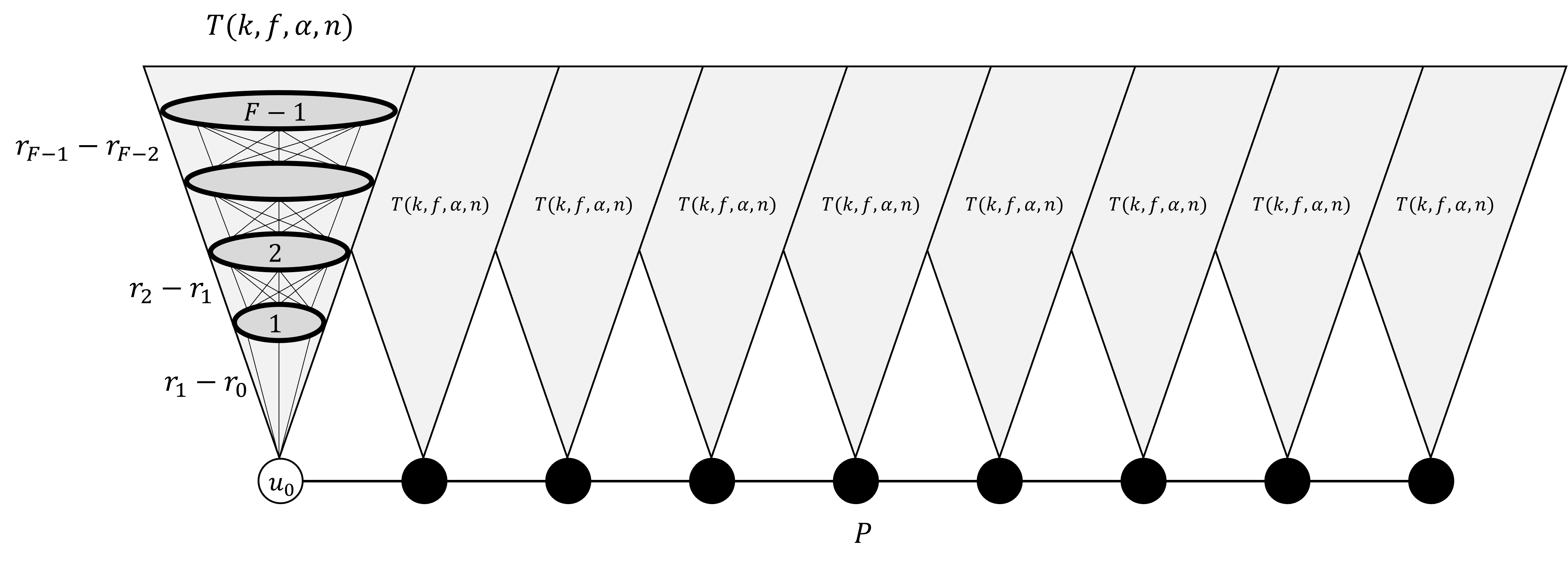
Figure 3: The graph $G(k,f,\alpha,n)$. $P$ contains $n^{\frac{1}{2k}}$ vertices, each of them is the $0$’th layer of a copy of $T(k,f,\alpha,n)$.

6.2 A Lower Bound for $H(k,f)$

Suppose we build the hopset $H(k,f)$ on the graph $G(k,f,\alpha,n)$. We prove the following lemma:

Lemma 14.

With high probability, for each $c\in[1,n^{\frac{1}{2k}}]$ and each $j<F-1$, $L_{c,j}$ contains a vertex from $A_{j}$, but doesn’t contain a vertex from $A_{j+1}$.

Proof.

We want to compute the probability that for every $c\in[1,n^{\frac{1}{2k}}]$ and $j\in[0,F-2]$,
$L_{c,j}\cap A_{j}\neq\emptyset\text{ and }L_{c,j}\cap A_{j+1}=\emptyset$. Since each vertex of the graph is chosen into the $A_{j}$’s independently, we get that the events $(L_{c,j}\cap A_{j}\neq\emptyset\text{ and }L_{c,j}\cap A_{j+1}=\emptyset)$ for different $c$’s and $j$’s are independent. Also, notice that if $L_{c,j}\cap A_{j}=\emptyset$, then $L_{c,j}\cap A_{j+1}=\emptyset$ as well, since $A_{j+1}\subseteq A_{j}$, and therefore:

$$Pr[L_{c,j}\cap A_{j}\neq\emptyset\text{ and }L_{c,j}\cap A_{j+1}=\emptyset] = Pr[L_{c,j}\cap A_{j+1}=\emptyset]-Pr[L_{c,j}\cap A_{j}=\emptyset\text{ and }L_{c,j}\cap A_{j+1}=\emptyset]$$

$$= Pr[L_{c,j}\cap A_{j+1}=\emptyset]-Pr[L_{c,j}\cap A_{j}=\emptyset]\leavevmode\nobreak\ .$$

Then:

$$Pr[\forall_{c,j}\;L_{c,j}\cap A_{j}\neq\emptyset\text{ and }L_{c,j}\cap A_{j+1}=\emptyset] = \big{(}\prod_{j<F-1}Pr[L_{1,j}\cap A_{j}\neq\emptyset\text{ and }L_{1,j}\cap A_{j+1}=\emptyset]\big{)}^{n^{\frac{1}{2k}}}$$

$$= \prod_{j<F-1}(Pr[L_{1,j}\cap A_{j+1}=\emptyset]-Pr[L_{1,j}\cap A_{j}=\emptyset])^{n^{\frac{1}{2k}}}\leavevmode\nobreak\ .$$

Note that

$$Pr[L_{1,j}\cap A_{j}=\emptyset]=(1-n^{-\frac{1}{k}\sum_{l<j}\lambda_{l}})^{\log_{2}(n)n^{\frac{1}{k}\sum_{l<j}\lambda_{l}}}\leq e^{-\log_{2}(n)}<\frac{1}{n}\leavevmode\nobreak\ .$$

Also, by Markov inequality,

$$Pr[L_{1,j}\cap A_{j+1}=\emptyset] = 1-Pr[L_{1,j}\cap A_{j+1}\neq\emptyset]$$

$$= 1-Pr[|L_{1,j}\cap A_{j+1}|\geq 1]$$

$$\geq 1-\frac{{\mathbb{E}}[|L_{1,j}\cap A_{j+1}|]}{1}$$

$$= 1-\log_{2}(n)n^{\frac{1}{k}\sum_{l<j}\lambda_{l}}\cdot n^{-\frac{1}{k}\sum_{l<j+1}\lambda_{l}}$$

$$= 1-\log_{2}(n)n^{-\frac{\lambda_{j+1}}{k}}$$

$$\geq 1-\log_{2}(n)n^{-\frac{1}{k}}\leavevmode\nobreak\ .$$

So finally:

$$Pr[\forall_{c,j}\;L_{c,j}\cap A_{j}\neq\emptyset\text{ and }L_{c,j}\cap A_{j+1}=\emptyset] \geq (1-\log_{2}(n)n^{-\frac{1}{k}}-\frac{1}{n})^{(F-1)n^{\frac{1}{2k}}}$$

$$\geq (1-2\log_{2}(n)n^{-\frac{1}{k}})^{kn^{\frac{1}{2k}}}$$

$$\geq (1-2n^{-\frac{1}{k}+\frac{1}{4k}})^{kn^{\frac{1}{2k}}}$$

$$= (1-2n^{-\frac{3}{4k}})^{kn^{\frac{1}{2k}}}$$

$$\geq e^{-4n^{-\frac{3}{4k}}\cdot kn^{\frac{1}{2k}}}$$

$$= e^{-4kn^{-\frac{1}{4k}}}\stackrel{{\scriptstyle n\rightarrow\infty}}{{\longrightarrow}}1\leavevmode\nobreak\ ,$$

where we used the fact that $F\leq k+1$ (because $\forall_{l}\;\lambda_{l}\geq 1$, so $\sum_{l<k+1}\lambda_{l}\geq k+1$), and that $\frac{1}{n}\leq\log_{2}(n)n^{-\frac{1}{k}}$ and $\log_{2}(n)\leq n^{\frac{1}{4k}}$ for a large enough $n$. Also, we used the inequality:

$$\forall_{x\in[0,1]}\;\;1-\frac{x}{2}\geq e^{-x}\leavevmode\nobreak\ .$$

∎

Lemma 14 lets us understand what hop-edges $H(k,f)$ adds to $G(k,f,\alpha,n)$. We prove that each of these edges is either within the same copy of a tower, or has a large weight with respect to the number of towers it skips.

Lemma 15.

Let $k,f,\alpha,n$ and assume that lemma 14 is satisfied. Suppose that $H(k,f)$ contains an edge $(x,y)$, where $x\in L_{c,i}$, $y\in L_{d,j}$, $c\neq d$ and $i\leq j<F-2$. Then:

$$w(x,y)>(\alpha+1)(|d-c|-2)\leavevmode\nobreak\ .$$

Proof.

By the construction of $G(k,f,\alpha,n)$ we can see that the shortest path from $x$ to $y$ starts by getting from $x$ to the $0$’th layer of its tower, then through the path $P$, reaching the $0$’th layer of $y$’s tower, and finally getting up through the layers to $y$. Then, $w(x,y)$ is the weight of this shortest path, which is:

$$w(x,y)=\sum_{l<i}(r_{l+1}-r_{l})+|d-c|+\sum_{l<j}(r_{l+1}-r_{l})=r_{i}+|d-c|+r_{j}-2\leavevmode\nobreak\ .$$ (6)

Notice that by the definition of $H(k,f)$, for $x,y$ to be connected, one of the following must hold (see section 3 for the definitions of $H(k,f)$ and other notations):

1. $y=p_{j^{\prime}}(x)$ for some $j^{\prime}$.

2. $y\in B_{j^{\prime}}(x)$ for some $j^{\prime}\in[i^{\prime},f(i^{\prime})]$, where $i^{\prime}=i(x)$.

By lemma 14, we can assume that $L_{d,j}$, which contains $y$, doesn’t contain any vertex of level greater than $j$, so in both cases above, $j^{\prime}\leq j<F-2$. By the same lemma, $L_{c,j^{\prime}}$ contains some vertex from $A_{j^{\prime}}$, and since this layer is closer to $x$ than $L_{d,j}$ (which is in $y$’s tower), it cannot be that $p_{j^{\prime}}(x)$ is in a different tower. Therefore the first case is impossible, so the second case holds.

Since $y\in B_{j^{\prime}}(x)$, we know that $j^{\prime}=i(y)$: notice that by definition, $B_{j^{\prime}}(x)$ contains only vertices of $A_{j^{\prime}}$ that are strictly closer to $x$ than $p_{j^{\prime}+1}(x)$; so $y\in A_{j^{\prime}}$, but $y\notin A_{j^{\prime}+1}$ because otherwise $d(x,y)\geq d(x,p_{j^{\prime}+1}(x))$.

If $j^{\prime}<j$, then since the layer $L_{c,j^{\prime}+1}$ is closer to $x$ than $L_{d,j}$, and contains a vertex of level $j^{\prime}+1$, the distance between $x$ to $y$ is at least the distance from $x$ to $p_{j^{\prime}+1}(x)$, in contradiction to $y$ being in $B_{j^{\prime}}(x)$. Hence, $j^{\prime}=j$.

Again by lemma 14, the $(j+1)$’th layer of each tower contains a vertex of level $j+1$, but no layer beneath the $(j+1)$’th can contain such vertex. Therefore $p_{j+1}(x)$ must be in $L_{c,j+1}$, so the distance between $x$ and its $(j+1)$’th pivot is the distance between $L_{c,i}$ and $L_{c,j+1}$:

$$d(x,p_{j+1}(x))=\sum_{l=i}^{j}(r_{l+1}-r_{l})=r_{j+1}-r_{i}\leavevmode\nobreak\ .$$

Since $y\in B_{j^{\prime}}(x)=B_{j}(x)$, we get that $d(x,y)<d(x,p_{j+1}(x))$, i.e.:

$$w(x,y)=r_{i}+|d-c|+r_{j}-2<r_{j+1}-r_{i}\leavevmode\nobreak\ .$$

Notice that the layer $L_{c,i}$, which contains $x$, cannot contain a vertex of level greater than $i$, so $i^{\prime}\leq i$. We also know that $j\in[i^{\prime},f(i^{\prime})]$, so by $f^{-1}$’s definition: $f^{-1}(j)\leq i^{\prime}\leq i$. After rearranging the inequality above, we get:

$$|d-c|<r_{j+1}-r_{j}-2r_{i}+2\leq r_{j+1}-r_{j}-2r_{f^{-1}(j)}+2=\frac{1}{\alpha}(r_{j}+r_{f^{-1}(j)})+2\;\;\;\;\Rightarrow$$

$$\Rightarrow\;\;r_{j}+r_{f^{-1}(j)}>\alpha|d-c|-2\alpha\leavevmode\nobreak\ ,$$

where we used $\{r_{j}\}$’s definition and the fact that it’s a non-decreasing sequence. By these same reasons we finally get:

$$w(x,y) = r_{i}+|d-c|+r_{j}-2$$

$$\geq r_{f^{-1}(j)}+|d-c|+r_{j}-2$$

$$> \alpha|d-c|-2\alpha+|d-c|-2$$

$$= (\alpha+1)(|d-c|-2)\leavevmode\nobreak\ .$$

∎

We now show that the graph $G(k,f,\alpha,n)$ demonstrates a lower bound for the hopset $H(k,f)$. The following lemma shows that the upper bound for the hopbound of $H(k,f)$ from theorem 3 is actually tight, up to a $\Theta(\alpha^{2})$-factor.

Lemma 16.

Suppose that $H=H(k,f)$ is an $(\alpha,\beta)$-hopset for $G=G(k,f,\alpha,n)$. Then, if $n$ is large enough, with high probability:

$$\beta\geq\frac{r_{F-2}-1}{5\alpha^{2}}\leavevmode\nobreak\ .$$

Proof.

Denote by $u_{0}$ the first vertex of the path $P$ and let $v$ be some other vertex in this path. Let $P_{u_{0},v}$ be the shortest path between $u_{0},v$ in the graph $G\cup H$, that has at most $\beta$ edges. By our assumption that $H$ is an $(\alpha,\beta)$-hopset for $G$, we know that:

$$w(P_{u_{0},v})\leq\alpha d(u_{0},v)\leavevmode\nobreak\ .$$

We denote by $(x_{1},y_{1}),(x_{2},y_{2}),...,(x_{b},y_{b})$ all of the edges of $P_{u_{0},v}$ that connects two different towers in $G$. We denote by $(c_{1},d_{1}),(c_{2},d_{2}),...,(c_{b},d_{b})$ the respective tower indices of the vertices. In this notation, we assume that $y_{i}$ is always the vertex in the higher layer (i.e. if $x_{i}\in L_{c_{i},j^{\prime}}$ and $y_{i}\in L_{d_{i},j}$, then $j^{\prime}\leq j$). The index of the layer of $y_{i}$ is denoted by $j_{i}$ ($y_{i}\in L_{d_{i},j_{i}}$). Note that $b\leq\beta$, since $P_{u_{0},v}$ has at most $\beta$ edges.

Suppose at first that $\forall_{i}\;j_{i}<F-2$. Then, by Lemma 15, for every $i$ such that $(x_{i},y_{i})\in H$:

$$w(x_{i},y_{i})>(\alpha+1)(|d_{i}-c_{i}|-2)\leavevmode\nobreak\ .$$

For the other edges on this list ($i$’s such that $(x_{i},y_{i})\notin H$), it must be that $(x_{i},y_{i})\in G$, and since the only edges of $G$ that connect two different towers are between adjacent towers, we have $|d_{i}-c_{i}|=1$. Therefore, in that case we have:

$$w(x_{i},y_{i})=1>-\alpha-1=(\alpha+1)(|d_{i}-c_{i}|-2)$$

as well.

The weight of $P_{u_{0},v}$ is at least the sum of the weights of the edges $\{(x_{i},y_{i})\}$:

$$\alpha d(u_{0},v) \geq w(P_{u_{0},v})$$

$$\geq \sum_{i=1}^{b}w(x_{i},y_{i})$$

$$> (\alpha+1)\sum_{i=1}^{b}(|d_{i}-c_{i}|-2)$$

$$\geq (\alpha+1)(d(u_{0},v)-2b)$$

$$\geq (\alpha+1)(d(u_{0},v)-2\beta)\leavevmode\nobreak\ ,$$

where we used the fact that $\sum_{i=1}^{b}|d_{i}-c_{i}|\geq d(u_{0},v)$, which is true since $\{(x_{i},y_{i})\}$ are all of the edges of $P_{u_{0},v}$ that connect two different towers (other edges doesn’t make any ”progress” towards $v$).

Therefore, we got:

$$\alpha d(u_{0},v)>(\alpha+1)(d(u_{0},v)-2\beta)\;\;\Rightarrow\;\;d(u_{0},v)<2\beta(\alpha+1)\leq 4\alpha\beta\leavevmode\nobreak\ .$$

But, if we choose $v\in P$ such that $d(u_{0},v)=\lceil 4\alpha\beta\rceil$, we get a contradiction, and therefore our assumption that $\forall_{i}\;j_{i}<F-2$ can’t be true (here we assume that $n$ is large enough such that $n^{\frac{1}{2k}}>\lceil 4\alpha\beta\rceil$, so such vertex $v$ exists).

Now, for the specified $v\in P$ such that $d(u_{0},v)=\lceil 4\alpha\beta\rceil$, we know that there is some $i$ such that $j_{i}\geq F-2$, which means that:

$$5\alpha^{2}\beta\geq\alpha\lceil 4\alpha\beta\rceil=\alpha d(u_{0},v)\geq w(P_{u_{0},v})\geq w(x_{i},y_{i})\geq\sum_{l<F-2}(r_{l+1}-r_{l})=r_{F-2}-1\leavevmode\nobreak\ .$$

See equation (6) for the weight of the edge $(x_{i},y_{i})$.

We finally got that if $H(k,f)$ is an $(\alpha,\beta)$-hopset for $G(k,f,\alpha,n)$, then:

$$\beta\geq\frac{r_{F-2}-1}{5\alpha^{2}}\leavevmode\nobreak\ .$$

∎

The following lemma lets us understand better the lower bound that was found in the previous lemma:

Lemma 17.

For every $k,f$ and $\alpha\geq 2$:

$$r_{F-2}\geq\frac{1}{8}k^{1+\frac{1}{2\log\alpha}}\leavevmode\nobreak\ .$$

Proof.

We write again the definitions of $\{\lambda_{j}\},F,\{r_{j}\}$:

1. $\lambda_{j}=1+\sum_{l<f^{-1}(j)}\lambda_{l}$,

2. $F=\min\{F^{\prime}\;|\;\sum_{l<F^{\prime}}\lambda_{l}\geq k+1\}$,

3. $r_{0}=1$ and $r_{j+1}=(2+\frac{1}{\alpha})r_{j}+(2+\frac{1}{\alpha})r_{f^{-1}(j)}$.

Define a new sequence $\{\Lambda_{j}\}$ as follows:

$$\Lambda_{j}=1+\sum_{l<j}\lambda_{l}\leavevmode\nobreak\ .$$

We can immediately see by $\{\lambda_{j}\}$’s definition that $\Lambda_{f^{-1}(j)}=\lambda_{j}$, and therefore:

$$\Lambda_{j+1}=1+\sum_{l<j+1}\lambda_{l}=1+\sum_{l<j}\lambda_{l}+\lambda_{j}=\Lambda_{j}+\Lambda_{f^{-1}(j)}\leavevmode\nobreak\ .$$

By $F$’s definition, we get that $\Lambda_{F}=1+\sum_{l<F}\lambda_{l}\geq k+2$. It will later be useful to notice that:

$$\Lambda_{j+1}=\Lambda_{j}+\Lambda_{f^{-1}(j)}\leq 2\Lambda_{j}\;\;\Rightarrow\;\;\Lambda_{F-2}\geq\frac{1}{2}\Lambda_{F-1}\geq\frac{1}{4}\Lambda_{F}\geq\frac{k+2}{4}\leavevmode\nobreak\ .$$

We now try to find some $d>0$ such that we can prove the inequality $r_{j}\geq\Lambda_{j}^{1+\frac{1}{d}}$ for every $j\geq 0$. If we find such $d$, we will get:

$$r_{F-2}\geq\Lambda_{F-2}^{1+\frac{1}{d}}\geq(\frac{k+2}{4})^{1+\frac{1}{d}}\leavevmode\nobreak\ ,$$

which is similar to what we want to prove.

Suppose we prove this inequality by induction over $j$. For $j=0$, we have $r_{0}=1=1^{1+\frac{1}{d}}=\Lambda_{0}^{1+\frac{1}{d}}$, and for $j>0$:

$$r_{j} = (1+\frac{1}{\alpha})r_{j-1}+(2+\frac{1}{\alpha})r_{f^{-1}(j-1)}$$

$$\geq (1+\frac{1}{\alpha})\Lambda_{j-1}^{1+\frac{1}{d}}+(2+\frac{1}{\alpha})\Lambda_{f^{-1}(j-1)}^{1+\frac{1}{d}}$$

$$\stackrel{{\scriptstyle?}}{{\geq}} (\Lambda_{j-1}+\Lambda_{f^{-1}(j-1)})^{1+\frac{1}{d}}$$

$$= \Lambda_{j}^{1+\frac{1}{d}}\leavevmode\nobreak\ ,$$

So we are only left to prove the inequality marked by ”?”. In appendix B we prove that given $d>0$ such that $(1+\frac{1}{\alpha})^{-d}+(2+\frac{1}{\alpha})^{-d}\leq 1$:

$$\forall_{x,y\geq 0}\;(1+\frac{1}{\alpha})x^{1+\frac{1}{d}}+(2+\frac{1}{\alpha})y^{1+\frac{1}{d}}\geq(x+y)^{1+\frac{1}{d}}\leavevmode\nobreak\ .$$

Therefore, if we show that we can choose $d=2\log\alpha$, i.e. that $(1+\frac{1}{\alpha})^{-2\log\alpha}+(2+\frac{1}{\alpha})^{-2\log\alpha}\leq 1$, then our proof by induction holds, and we have:

$$r_{F-2}\geq\Lambda_{F-2}^{1+\frac{1}{2\log\alpha}}\geq(\frac{k+2}{4})^{1+\frac{1}{2\log\alpha}}\geq\frac{1}{8}k^{1+\frac{1}{2\log\alpha}}\leavevmode\nobreak\ ,$$

where the last inequality holds for every $\alpha\geq 2$.

For $\alpha\geq 2$, we have $\alpha^{2}\geq 2\alpha$, and then $2\alpha+1\leq\alpha^{2}+1<2\alpha^{2}<2\alpha^{3}$.

Now, for $\alpha\geq 2$:

$$(1+\frac{1}{\alpha})^{-2\log\alpha}+(2+\frac{1}{\alpha})^{-2\log\alpha} \leq (1+\frac{1}{\alpha})^{-2}+2^{-2\log\alpha}$$

$$= \frac{\alpha^{2}}{(\alpha+1)^{2}}+\frac{1}{\alpha^{2}}$$

$$= \frac{\alpha^{4}+(\alpha+1)^{2}}{\alpha^{2}(\alpha+1)^{2}}$$

$$= \frac{\alpha^{4}+\alpha^{2}+2\alpha+1}{\alpha^{4}+2\alpha^{3}+\alpha^{2}}$$

$$< \frac{\alpha^{4}+\alpha^{2}+2\alpha^{3}}{\alpha^{4}+2\alpha^{3}+\alpha^{2}}$$

$$= 1$$

∎

The following theorem concludes the previous two lemmas:

Theorem 8.

For every choice of $k,f$ and $\alpha\geq 2$, there is a graph $G$ such that if the hopset $H(k,f)$ is an $(\alpha,\beta)$-hopset for $G$, then with high probability:

$$\beta\geq\frac{1}{40\alpha^{2}}k^{1+\frac{1}{2\log\alpha}}-1\leavevmode\nobreak\ .$$

Proof.

Fix some $k,f$, and let $n\in\{2^{2k\cdot a}\;|\;a\in\mathbb{N}\}$ be large enough such that the previous lemmas are true (particularly, choose $n$ such that lemma 14 and lemma 16 are satisfied). When choosing $G=G(k,f,\alpha,n)$, we know by lemma 16 that $\beta\geq\frac{r_{F-2}-1}{5\alpha^{2}}$, and by lemma 17 that $r_{F-2}\geq\frac{1}{8}k^{1+\frac{1}{2\log\alpha}}$. Combining these two results, we get:

$$\beta\geq\frac{1}{5\alpha^{2}}(r_{F-2}-1)\geq\frac{1}{5\alpha^{2}}(\frac{1}{8}k^{1+\frac{1}{2\log\alpha}}-1)\geq\frac{1}{40\alpha^{2}}k^{1+\frac{1}{2\log\alpha}}-1\leavevmode\nobreak\ .$$

∎

Remark 3.

While we achieved a lower bound of $\beta=\Omega(\frac{1}{\alpha^{2}}k^{1+1/2\log\alpha})$ for the hopbound of $H(k,f)$, we believe that a lower bound of $\beta=\Omega(\frac{1}{\alpha}k^{1+1/2\log\alpha})$ may also be shown. If such lower bound is achieved, notice that it would be tight compared to the known upper bounds for various values of $\alpha$:

1. For $\alpha=\Theta(k^{\epsilon})$, for a constant $0<\epsilon\leq 1$, we know that with a suitable choice of $f$, $H(k,f)$ has a hopbound of $O(k^{1-\epsilon})$ (see subsection 4.1.3). The lower bound in this case would be:

   $$\beta=\Omega(\frac{1}{\alpha}k^{1+1/2\log\alpha})=\Omega_{\epsilon}(k^{1-\epsilon})\leavevmode\nobreak\ .$$

2. For $\alpha=O(1)$, with a suitable choice of $f$, $H(k,f)$ has a hopbound of $O(k^{1+\frac{2}{\ln\alpha}})$ (see subsection 4.1.2). The lower bound in this case would be:

   $$\beta=\Omega(k^{1+1/2\log\alpha})\leavevmode\nobreak\ .$$

For $\alpha=O(1)$, notice that our lower bound from theorem 8 is also tight, since $O(\frac{1}{\alpha^{2}})=O(\frac{1}{\alpha})=O(1)$.

Appendix A Estimating $r_{F}$ for $f(i)=\lfloor\frac{i}{c}\rfloor\cdot c+c-1$

Given the function $f(i)=\lfloor\frac{i}{c}\rfloor\cdot c+c-1$, we saw in subsection 4.1.2 that $\lambda_{ic+j}=(c+1)^{i}$ for every $i$ and $j\in[0,c-1]$. We now want to estimate $r_{F}$, for the minimal $F$ such that $\sum_{l<F}\lambda_{l}\geq k+1$, where $\{r_{i}\}$ is a sequence that satisfies:

$$\forall_{i>0}\;r_{i}=(1+\frac{4}{t})r_{i-1}+(2+\frac{4}{t})r_{f^{-1}(i-1)}\leavevmode\nobreak\ .$$

Suppose that $F=i_{F}\cdot c+j_{F}$ where $j_{F}\in[1,c]$ - Note that here, if $F$ is divisible by $c$, say $F=q\cdot c$, we write it as $F=(q-1)c+c$ instead of $F=qc+0$. Then:

$$\sum_{l<F}\lambda_{l} = \sum_{l<i_{F}\cdot c}\lambda_{l}+\sum_{l=i_{F}\cdot c}^{F-1}\lambda_{l}$$

$$= \sum_{i<i_{F}}c(c+1)^{i}+\sum_{l=i_{F}\cdot c}^{F-1}(c+1)^{i_{F}}$$

$$= c\cdot\frac{(c+1)^{i_{F}}-1}{(c+1)-1}+(F-i_{F}\cdot c)(c+1)^{i_{F}}$$

$$= (c+1)^{i_{F}}-1+j_{F}(c+1)^{i_{F}}$$

$$= (j_{F}+1)(c+1)^{i_{F}}-1\leavevmode\nobreak\ .$$

The last $\lambda_{l}$ in the sum is $\lambda_{F-1}=\lambda{i_{F}\cdot c+j_{F}-1}=(c+1)^{i_{F}}$, since $j_{F}\in[1,c]$. Subtracting it from both sides, we get:

$$\sum_{l<F-1}\lambda_{l}=j_{F}(c+1)^{i_{F}}-1\leavevmode\nobreak\ .$$

$F$ is minimal such that $\sum_{l<F}\lambda_{l}\geq k+1$, so it must be that:

$$(j_{F}+1)(c+1)^{i_{F}}\geq k+2\leavevmode\nobreak\ ,$$

and

$$j_{F}(c+1)^{i_{F}}<k+2$$ (7)

Notice that $\lceil\log_{c+1}(k+2)\rceil c$ is an upper bound for $F$, since:

$$\sum_{j<\lceil\log_{c+1}(k+2)\rceil c}\lambda_{j}=\sum_{l<\lceil\log_{c+1}(k+2)\rceil}c(c+1)^{l}=(c+1)^{\lceil\log_{c+1}(k+2)\rceil}-1\geq k+1\leavevmode\nobreak\ .$$

Therefore, we know that:

$$i_{F}\leq\lceil\log_{c+1}(k+2)\rceil\leavevmode\nobreak\ .$$

Now, we want to estimate $r_{F}$. By the same proof from subsection 4.1.2, we get:

$$r_{ic+j}=[(1+\frac{1}{c})^{j}(2c+2)-(2c+1)]r_{ic}\leavevmode\nobreak\ ,$$

$$r_{ic}=[(1+\frac{1}{c})^{c}(2c+2)-(2c+1)]^{i}r_{0}\leavevmode\nobreak\ .$$

So we get:

$$r_{F}=[(1+\frac{1}{c})^{j_{F}}(2c+2)-(2c+1)][(1+\frac{1}{c})^{c}(2c+2)-(2c+1)]^{i_{F}}r_{0}\leavevmode\nobreak\ .$$

We bound the first square brackets of $r_{F}$:

$$[(1+\frac{1}{c})^{j_{F}}(2c+2)-(2c+1)] = [(1+(1+\frac{1}{c})^{j_{F}}-1)(2c+2)-(2c+1)]$$

$$= (2c+2)-(2c+1)+[(1+\frac{1}{c})^{j_{F}}-1](2c+2)$$

$$= 1+[(1+\frac{1}{c})^{j_{F}}-1](2c+2)$$

$$\leq 1+[e^{\frac{j_{F}}{c}}-1]\cdot 3c$$

$$\leq 1+(e-1)\frac{j_{F}}{c}\cdot 3c$$

$$= 1+3(e-1)j_{F}\leavevmode\nobreak\ ,$$

where in the last inequality we used the fact that $\forall_{x\in[0,1]}\;e^{x}-1\leq(e-1)x$.

For the second square brackets of $r_{F}$, we use the inequality $(1+\frac{1}{c})^{c}\leq e$:

$$[(1+\frac{1}{c})^{c}(2c+2)-(2c+1)]^{i_{F}} \leq [2e(c+1)]^{i_{F}}\leq(2e)^{\lceil\log_{c+1}(k+2)\rceil}(c+1)^{i_{F}}$$

$$\leq 2e(2e)^{\log_{c+1}(k+2)}(c+1)^{i_{F}}$$

$$\leq 2e(k+2)^{\frac{\ln(2e)}{\ln(c+1)}}(c+1)^{i_{F}}$$

$$\leq 2e\cdot 2^{\frac{\ln(2e)}{\ln(c+1)}}k^{\frac{\ln(2e)}{\ln(c+1)}}(c+1)^{i_{F}}$$

$$\leq 16ek^{\frac{2}{\ln c}}(c+1)^{i_{F}}\leavevmode\nobreak\ .$$

So we finally get:

$$r_{F}\leq[1+3(e-1)j_{F}][16ek^{\frac{2}{\ln c}}(c+1)^{i_{F}}]r_{0}\leavevmode\nobreak\ .$$

Recall that $j_{F}\geq 1$ and therefore $1+3(e-1)j_{F}\leq(3e-2)j_{F}$. By inequality (7) we get:

$$r_{F} \leq (3e-2)\cdot 16ek^{\frac{2}{\ln c}}j_{F}(c+1)^{i_{F}}\cdot r_{0}$$

$$\leq 48e^{2}k^{\frac{2}{\ln c}}(k+1)\cdot r_{0}$$

$$\leq 96e^{2}k^{\frac{2}{\ln c}}k\cdot r_{0}$$

$$= 96e^{2}k^{1+\frac{2}{\ln c}}\cdot r_{0}\leavevmode\nobreak\ .$$

Appendix B Completing the Proof of Lemma 17

For completing the proof of the lemma 17, we prove the following lemma:

Lemma 18.

For any $a,b>1$, $d>0$, such that $a^{-d}+b^{-d}\leq 1$:

$$\forall_{x,y\geq 0}\;\;ax^{1+\frac{1}{d}}+by^{1+\frac{1}{d}}\geq(x+y)^{1+\frac{1}{d}}\leavevmode\nobreak\ .$$

Proof.

For a fixed $y\geq 0$, define a function:

$$h(x)=ax^{1+\frac{1}{d}}+by^{1+\frac{1}{d}}-(x+y)^{1+\frac{1}{d}}$$

We want to show that for every $x\geq 0$, $h(x)\geq 0$.

Derive $h$:

$$h^{\prime}(x)=a(1+\frac{1}{d})x^{\frac{1}{d}}-(1+\frac{1}{d})(x+y)^{\frac{1}{d}}=(1+\frac{1}{d})x^{\frac{1}{d}}(a-(1+\frac{y}{x})^{\frac{1}{d}})$$

In $[0,\infty)$, the derivative is positive when $a>(1+\frac{y}{x})^{\frac{1}{d}}$, i.e. $x>\frac{y}{a^{d}-1}$, negative when $0<x<\frac{y}{a^{d}-1}$, and equals zero when $x=0$ or $x=\frac{y}{a^{d}-1}$. That means that $x=\frac{y}{a^{d}-1}$ is the global minimum of $h$ in $[0,\infty)$, i.e. $\forall_{x\geq 0}\;h(x)\geq h(\frac{y}{a^{d}-1})$.

Compute $h(\frac{y}{a^{d}-1})$:

$$h(\frac{y}{a^{d}-1}) = \frac{a}{(a^{d}-1)^{1+\frac{1}{d}}}y^{1+\frac{1}{d}}+by^{1+\frac{1}{d}}-(\frac{1}{a^{d}-1}+1)^{1+\frac{1}{d}}y^{1+\frac{1}{d}}$$

$$= [\frac{a}{(a^{d}-1)^{1+\frac{1}{d}}}+b-(\frac{a^{d}}{a^{d}-1})^{1+\frac{1}{d}}]y^{1+\frac{1}{d}}$$

$$= [b+\frac{a-a^{d}\cdot a}{(a^{d}-1)^{1+\frac{1}{d}}}]y^{1+\frac{1}{d}}$$

$$= [b-a(a^{d}-1)^{-\frac{1}{d}}]y^{1+\frac{1}{d}}$$

So $h(\frac{y}{a^{d}-1})\geq 0$ iff

$$a(a^{d}-1)^{-\frac{1}{d}}\leq b\;\;\iff\;\;\frac{a^{d}}{a^{d}-1}\leq b^{d}\;\;\iff\;\;a^{d}+b^{d}\leq a^{d}b^{d}\;\;\iff\;\;a^{-d}+b^{-d}\leq 1$$

∎

References

- [ABP17] Amir Abboud, Greg Bodwin, and Seth Pettie. A hierarchy of lower bounds for sublinear additive spanners. In Proceedings of the Twenty-Eighth Annual ACM-SIAM Symposium on Discrete Algorithms, SODA 2017, Barcelona, Spain, Hotel Porta Fira, January 16-19, pages 568–576, 2017.
- [ADD+93] I. Althöfer, G. Das, D. Dobkin, D. Joseph, and J. Soares. On sparse spanners of weighted graphs. Discrete Comput. Geom., 9:81–100, 1993.
- [Ber09] Aaron Bernstein. Fully dynamic (2 + epsilon) approximate all-pairs shortest paths with fast query and close to linear update time. In 50th Annual IEEE Symposium on Foundations of Computer Science, FOCS 2009, October 25-27, 2009, Atlanta, Georgia, USA, pages 693–702, 2009.
- [BKMP10] Surender Baswana, Telikepalli Kavitha, Kurt Mehlhorn, and Seth Pettie. Additive spanners and (alpha, beta)-spanners. ACM Transactions on Algorithms, 7(1):5, 2010.
- [BLP20] Uri Ben-Levy and Merav Parter. New (a, ß) spanners and hopsets. In Proceedings of the Thirty-First Annual ACM-SIAM Symposium on Discrete Algorithms, SODA ’20, pages 1695–1714, USA, 2020. Society for Industrial and Applied Mathematics.
- [Coh00] Edith Cohen. Polylog-time and near-linear work approximation scheme for undirected shortest paths. J. ACM, 47(1):132–166, 2000.
- [EGN19] Michael Elkin, Yuval Gitlitz, and Ofer Neiman. Almost shortest paths with near-additive error in weighted graphs. CoRR, abs/1907.11422, 2019.
- [Elk04] M. Elkin. An unconditional lower bound on the time-approximation tradeoff of the minimum spanning tree problem. In Proc. of the 36th ACM Symp. on Theory of Comput. (STOC 2004), pages 331–340, 2004.
- [EN16] Michael Elkin and Ofer Neiman. Hopsets with constant hopbound, and applications to approximate shortest paths. In IEEE 57th Annual Symposium on Foundations of Computer Science, FOCS 2016, 9-11 October 2016, Hyatt Regency, New Brunswick, New Jersey, USA, pages 128–137, 2016.
- [EN19] Michael Elkin and Ofer Neiman. Linear-size hopsets with small hopbound, and constant-hopbound hopsets in RNC. In The 31st ACM on Symposium on Parallelism in Algorithms and Architectures, SPAA 2019, Phoenix, AZ, USA, June 22-24, 2019., pages 333–341, 2019.
- [EP04] Michael Elkin and David Peleg. (1+epsilon, beta)-spanner constructions for general graphs. SIAM J. Comput., 33(3):608–631, 2004.
- [EP15] Michael Elkin and Seth Pettie. A linear-size logarithmic stretch path-reporting distance oracle for general graphs. In Proceedings of the Twenty-Sixth Annual ACM-SIAM Symposium on Discrete Algorithms, SODA 2015, San Diego, CA, USA, January 4-6, 2015, pages 805–821, 2015.
- [FL16] Stephan Friedrichs and Christoph Lenzen. Parallel metric tree embedding based on an algebraic view on moore-bellman-ford. In Proceedings of the 28th ACM Symposium on Parallelism in Algorithms and Architectures, SPAA ’16, pages 455–466, New York, NY, USA, 2016. ACM.
- [HKN16] Monika Henzinger, Sebastian Krinninger, and Danupon Nanongkai. A deterministic almost-tight distributed algorithm for approximating single-source shortest paths. In Proceedings of the Forty-eighth Annual ACM Symposium on Theory of Computing, STOC ’16, pages 489–498, New York, NY, USA, 2016. ACM.
- [HP17] Shang-En Huang and Seth Pettie. Thorup-zwick emulators are universally optimal hopsets. Information Processing Letters, 142, 04 2017.
- [KS97] Philip N. Klein and Sairam Subramanian. A randomized parallel algorithm for single-source shortest paths. J. Algorithms, 25(2):205–220, 1997.
- [LPS88] Alexander Lubotzky, Ralph Phillips, and Peter Sarnak. Ramanujan graphs. Combinatorica, 8(3):261–277, 1988.
- [MPVX15] Gary L. Miller, Richard Peng, Adrian Vladu, and Shen Chen Xu. Improved parallel algorithms for spanners and hopsets. In Proceedings of the 27th ACM Symposium on Parallelism in Algorithms and Architectures, SPAA ’15, pages 192–201, New York, NY, USA, 2015. ACM.
- [Pet08] Seth Pettie. Distributed algorithms for ultrasparse spanners and linear size skeletons. In Proceedings of the Twenty-seventh ACM Symposium on Principles of Distributed Computing, PODC ’08, pages 253–262, New York, NY, USA, 2008. ACM.
- [Pet10] Seth Pettie. Distributed algorithms for ultrasparse spanners and linear size skeletons. Distributed Computing, 22(3):147–166, 2010.
- [PU89] David Peleg and Eli Upfal. A trade-off between space and efficiency for routing tables. J. ACM, 36(3):510–530, 1989.
- [TZ01] M. Thorup and U. Zwick. Approximate distance oracles. In Proc. of the 33rd ACM Symp. on Theory of Computing, pages 183–192, 2001.
- [TZ06] M. Thorup and U. Zwick. Spanners and emulators with sublinear distance errors. In Proc. of Symp. on Discr. Algorithms, pages 802–809, 2006.