Signed Bipartite Graph Neural Networks

Abstract.

Signed networks are such social networks having both positive and negative links. A lot of theories and algorithms have been developed to model such networks (e.g., balance theory). However, previous work mainly focuses on the unipartite signed networks where the nodes have the same type. Signed bipartite networks are different from classical signed networks, which contain two different node sets and signed links between two node sets. Signed bipartite networks can be commonly found in many fields including business, politics, and academics, but have been less studied. In this work, we firstly define the signed relationship of the same set of nodes and provide a new perspective for analyzing signed bipartite networks. Then we do some comprehensive analysis of balance theory from two perspectives on several real-world datasets. Specifically, in the peer review dataset, we find that the ratio of balanced isomorphism in signed bipartite networks increased after rebuttal phases. Guided by these two perspectives, we propose a novel Signed Bipartite Graph Neural Networks (SBGNNs) to learn node embeddings for signed bipartite networks. SBGNNs follow most GNNs message-passing scheme, but we design new message functions, aggregation functions, and update functions for signed bipartite networks. We validate the effectiveness of our model on four real-world datasets on  Link Sign Prediction task, which is the main machine learning task for signed networks. Experimental results show that our SBGNN model achieves significant improvement compared with strong baseline methods, including feature-based methods and network embedding methods.

ACM Reference Format:
Junjie Huang, Huawei Shen, Qi Cao, Shuchang Tao, Xueqi Cheng. 2021. Signed Bipartite Graph Neural Networks. In Proceedings of the 30th ACM International Conference on Information and Knowledge Management (CIKM ’21), November 1–5, 2021, Virtual Event, QLD, Australia. ACM, New York, NY, USA, 10 pages. https://doi.org/10.1145/3459637.3482392

1. Introduction

According to a well-known Asian proverb, “There are a thousand Hamlets in a thousand people’s eyes”. It means that different people have different opinions. These differences usually include both positive and negative attitudes. They are reflected in many fields including business, politics, and academics. For instance, a research paper submitted to CIKM may receive completely opposite reviews from two reviewers. Reviewer 1 gives an “Accept” decision, while Reviewer 2 chooses the “Reject” option. Understanding and modeling these differences is a useful perspective on a range of social computing studies (e.g., AI peer review (Heaven, 2018) and congressional vote prediction (Karimi et al., 2019)).

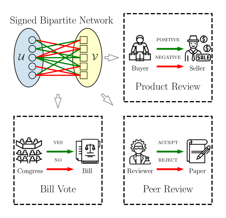
Figure 1. Common application scenarios for signed bipartite networks.

Figure 1 shows some common application scenarios for signed bipartite networks, including product review, bill vote, and peer review. Some opinions can be viewed as positive relationships, such as favorable reviews on products, supporting the bill, accepting a paper, and so on. Meanwhile, some opinions are negative links that indicate negative reviews, disapproving a bill, rejecting a paper, and so forth. These scenarios can be modeled as signed bipartite networks, which include two sets of nodes (i.e., $\mathcal{U}$ and $\mathcal{V}$) and the links with positive and negative relationships between two sets. Compared with unsigned bipartite networks, the links of signed bipartite networks are more complicated, including two opposite relationships (i.e., positive and negative links). Besides, previous works on signed networks only focus on unbipartite signed networks, which are networks that have a single node type (Facchetti et al., 2011). Different node types in signed bipartite networks represent different things. Modeling signed bipartite networks is a promising and challenging research field.

With modeling the above scenarios into signed bipartite net-works, we do social network analysis on real-world datasets and use advanced graph representation learning methods to model them. In signed networks, balance analysis is one of the key research problems in signed graph modeling (Huang et al., 2021a). A common balance analysis method is to count the number of balanced signed triangles in unbipartite signed networks (Leskovec et al., 2010b). For signed bipartite networks, (Derr et al., 2019) defines the signed butterfly isomorphism, and uses it to analyze the balance in signed bipartite networks. But signed butterfly isomorphism may be missing due to data sparsity. In this paper, we offer a new perspective for analyzing balance theory on signed bipartite networks. By sign construction, we construct the links between the nodes in the same set and count the signed triangles for the links between the nodes in the same set. We analyze the balance theory of signed bipartite networks from both two perspectives and explore the balance change in the peer review scenario. We find that after rebuttal, the balance of the review signed bipartite network increased. In addition to social network analysis, graph representation learning is another important tool. Graph Neural Networks (GNNs) have achieved state-of-art results in graph representation learning. Combing two perspectives, we propose a new Signed Bipartite Graph Neural Networks (SBGNNs). This model follows the message passing scheme, but we redesign the message function, aggregation function, and update function. Our SBGNN model achieves the state-of-art results on  Link Sign Prediction , which is the main machine learning task in signed networks (Derr et al., 2020). To the best of our knowledge, none of the existing GNN methods has paid special attention to signed bipartite networks. It’s the first time to introduce GNNs to signed bipartite networks. To summarize, the major contributions of this paper are as follows:

• By defining the signed relationship of the same set of nodes (e.g., agreement/disagreement), we provide a new perspective for analyzing signed bipartite networks, which can measure the unbalanced structure of the signed bipartite networks from the same set of nodes.

• Combining two perspectives, we introduce a new layer-by-layer SBGNN model. Via defining new message functions, aggregation functions, and update functions, SBGNNs aggregate information from neighbors in different node sets and output effective node representations.

• We conduct  Link Sign Prediction experiments on four real-world signed bipartite networks including product review, bill vote, and peer review. Experimental results demonstrate the effectiveness of our proposed model.

2. Related Work

2.1. Signed Graph Modeling

Signed networks are such social networks having both positive and negative links (Easley and Kleinberg, 2010). Balance theory (Heider, 1944; Cartwright and Harary, 1956) is the fundamental theory in the signed network field (Kirkley et al., 2019). For classical signed networks, signed triangles are the most common way to measure the balance of signed networks (Szell et al., 2010). Distinct from homogeneous networks, there are two types of nodes in in bipartite networks. For signed bipartite networks, (Derr et al., 2019) conducts the comprehensive analysis on balance theory in signed bipartite networks, using the smallest cycle in signed bipartite networks (i.e., signed butterflies).

To mine signed networks, many algorithms have been developed for lots of tasks, such as community detection (Traag and Bruggeman, 2009; Bonchi et al., 2019), node classification (Tang et al., 2016a), node ranking (Shahriari and Jalili, 2014), and spectral graph analysis (Li et al., 2018). The  Link Sign Prediction is the main machine learning task for signed networks (Song and Meyer, 2015). Modeling balance theory usually leads to better experimental results on  Link Sign Prediction  (Huang et al., 2021b). For example, (Leskovec et al., 2010a) extracts features by counting signed triangles and achieve good performance in  Link Sign Prediction . Even with recently signed network embedding methods (Wang et al., 2017; Chen et al., 2018; Mara et al., 2020; Javari et al., 2020), balance theory will be the important guideline for designing models. Specifically, SiNE (Wang et al., 2017) designs an objective function guided by balance theory to learn signed network embeddings and outperforms feature-based methods. For signed bipartite networks, how to incorporate balance theory is a research-worthy problem.

2.2. Graph Representation Learning

Graph Representation Learning (or Network Representation Learning) is to learn a mapping that embeds nodes, or entire (sub)graphs, as points in a low-dimensional vector space (Hamilton et al., 2017b). The nodes in the graph is represented as node embeddings, which reflect the structure of the origin graph. The common methods for graph representation learning include matrix factorization-based methods (Ou et al., 2016), random-walk based algorithms (Perozzi et al., 2014; Tang et al., 2015; Grover and Leskovec, 2016), and graph neural networks. Specifically, Node2vec (Grover and Leskovec, 2016) extends DeepWalk (Perozzi et al., 2014) by performing biased random walks to generate the corpus of node sequences; and it efficiently explores more diverse neighborhoods. For various complex networks (e.g., bipartite networks (Gao et al., 2018) and signed networks (Yuan et al., 2017)), researchers have also proposed a variety of embedding methods by adapting the random walk methods.

Recently, Graph neural networks (GNNs) have received tremendous attention due to the power in learning effective representations for graphs (Xu et al., 2019, 2018b). Most GNNs can be summarized as a message-passing scheme where the node representations are updated by aggregating and transforming the information from the neighborhood (Gilmer et al., 2017). GNNs have a partial intersection but use the deep learning methods instead of matrix factorization and random walk and can better describe the network structure (Wu et al., 2020). A lot of GNN models show a better performance than the shadow lookup embeddings (Kipf and Welling, 2019; Veličković et al., 2018; Hamilton et al., 2017a). Most GNNs are designed for unsigned social networks whose links are only positive. For signed networks, some signed GNNs (Derr et al., 2018; Huang et al., 2019) are proposed to model the balance theory using convolution or attention mechanism. But they cannot handle the signed bipartite networks, because there are no links between nodes in the same sets. It is not trivial to transfer these models to signed bipartite networks.

3. Balance Theory in Signed Bipartite Networks

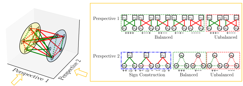
Figure 2. For a signed bipartite network, there exist two different analysis perspectives. Perspective 1 offers to analyze the signed butterfly isomorphism. For Perspective 2, we can analyze the signed triangle isomorphism by sign construction.

For signed networks, balance theory is one of the most fundamentally studied social theories, which is originated in social psychology in the 1950s (Heider, 1944). It discusses that due to the stress or psychological dissonance, people will strive to minimize the unbalanced state in their personal relationships, and hence they will change to balanced social settings. Specifically, triads with an even number of negative edges are defined as balanced. However, previous researches on balance theory are focused on unbipartite signed networks, measuring balance theory in signed bipartite networks is less studied. In this section, we give two perspectives to analyze balance theory in signed bipartite networks.

3.1. Signed Bipartite Networks

Table 1. Statistics on Signed Bipartite Networks.

	Bonanza	U.S. House	U.S. Senate	Preliminary Review	Final Review
$|\mathcal{U}|$	7,919	515	145	182	182
$|\mathcal{V}|$	1,973	1,281	1,056	304	304
$|\mathcal{E}|=|\mathcal{E}^{+}|+|\mathcal{E}^{-}|$	36,543	114,378	27,083	1,170	1,170
% Positive Links	0.980	0.540	0.553	0.403	0.397
% Negative Links	0.020	0.460	0.447	0.597	0.603

Firstly, we describe our datasets used in this paper. The first dataset is from the e-commerce website Bonanza, which is similar to eBay or Taobao. Users can purchase products from a seller and rate the seller with “Positive”, “Neutral”, or “Negative” scores. In this dataset, $\mathcal{U}$ represents the buyers, and $\mathcal{V}$ represents the sellers. The next two datasets (i.e., U.S. Senate and U.S. House) are from the 1st to 10th United States Congress vote records. It is collected from the Govtrack.us. The senators or representatives $\mathcal{U}$ can vote “Yea” or “Nay” for bills $\mathcal{V}$, which is the positive or negative links respectively. The above datasets are collected and used by (Derr et al., 2019). The last dataset is the peer review data from a top computer science conference. Reviewers $\mathcal{U}$ can give “SA” (Strong Accept), “A” (Accept), “WA” (Weak Accept), “WR” (Weak Reject), “R” (Reject), and “SR” (Strong Reject) to papers $\mathcal{V}$ after reviewing. We regard “SA”, “A”, and “WA” as positive links and “SR”, “R” and “WR” as negative links. It’s worth mentioning that in most computer science conference peer reviews, there is usually a rebuttal phase when authors can point out errors in the reviews and help clarify reviewers’ misunderstandings. It has proven to play a critical role in the final decision made by the meta-reviewers and the reviewers. Besides, during the rebuttal phase, the reviewers can see the scores of other reviewers and make adjustments to their review comments and scores based on the author’s response and other reviewers’ comments. Therefore, the peer review dataset is divided into two parts: Preliminary Review and Final Review.

We list the statistics of datasets in Table 1. From Table 1, we can find that in different scenarios, the negative ratio varies. In the scenario of product reviews, the ratio of negative links is relatively lower (i.e., 0.02). Buyers rarely give bad rates to sellers. In the scenario of bill vote, the proportion of negative links increases comparing to the scenario of product reviews (i.e., 0.460 and 0.447). In many bills, it is more difficult for legislators to reach consensus due to different political standpoints. In the scenario of peer reviews, the ratio of negative links is higher than the ratios of positive links (i.e., $0.603>0.397$). In the top conferences of computer science, the acceptance rate needs to be controlled (e.g., about 20% in CIKM), so reviewers usually raise their standards for reviewing the paper, which will have a greater probability of giving negative reviews. Surprisingly, after the rebuttal phase, the proportion of negative links has slightly risen (i.e., from 0.597 to 0.603).

3.2. Signed Caterpillars and Signed Butterflies

The “butterfly” is the most basic motif that models cohesion in an unsigned bipartite network, which is the complete 2×2 biclique (Sanei-Mehri et al., 2018). Base on the butterfly definition, (Derr et al., 2019) extends it to the signed butterfly by giving signs to the links in classical butterfly isomorphism. Except for signed butterfly definition, (Derr et al., 2019) denotes “signed caterpillars” as paths of length that are missing just one link to becoming a signed butterfly. They use signed butterflies to investigate balance theory in signed bipartite networks.

According to the definition of  (Derr et al., 2019), we use the notation $\bigcirc~{}\bigcirc~{}\bigcirc~{}\bigcirc$ to denote a signed butterfly isomorphism class that represents the links between $\mathcal{U}$ and $\mathcal{V}$ (i.e., $u_{1}\rightarrow^{\bigcirc}v_{1},u_{1}\rightarrow^{\bigcirc}v_{2},u_{2}\rightarrow^{\bigcirc}v_{1},u_{2}\rightarrow^{\bigcirc}v_{2}$). Due to the symmetry of the structure, we can get 7 non-isomorphic signed butterflies classes. We show them in Perspective 1 in Figure 2 and divide them into two categories, balanced and unbalanced. For example, isomorphism class ++++ and ---- denote the classes having all positive or all negative links, respectively. In the scenario of peer reviews, we can interpret isomorphism class ++++ as the situations where reviewer $u_{1}$ and reviewer $u_{2}$ both give “Accept” to paper $v_{1}$ and paper $v_{2}$ (i.e., $u_{1}\rightarrow^{+}v_{1},u_{1}\rightarrow^{+}v_{2},u_{2}\rightarrow^{+}v_{1},u_{2}\rightarrow^{+}v_{2}$). Similarly, we can interpret isomorphism class ---- as reviewer $u_{1}$ and reviewer $u_{2}$ both reject paper $v_{1}$ and paper $v_{2}$ (i.e., $u_{1}\rightarrow^{-}v_{1},u_{1}\rightarrow^{-}v_{2},u_{2}\rightarrow^{-}v_{1},u_{2}\rightarrow^{-}v_{2}$). Except isomorphism class ++++ and ----, isomorphism class ++--, +-+-, and ---- are balanced since they have an even number of negative links. In fact, the definition of signed butterflies can be viewed as analyzing the signed bipartite network from Perspective 1.

3.3. Signed Triangles in Signed Bipartite Networks

For signed bipartite networks, the nodes of the same set are not connected. Therefore, we propose a new sign construction process by judging the sign of the link from $\mathcal{U}$ to $\mathcal{V}$. After sign construction, we have signed links between nodes in the same set. It means that we have two new signed networks for $\mathcal{U}$ and $\mathcal{V}$ after sign construction.

As shown in Perspective 2 in Figure 2, when $u_{1}$ and $u_{2}$ have links with same sign on $v_{1}$ (i.e., , $u_{1}\rightarrow^{+}v_{1},u_{2}\rightarrow^{+}v_{1}$ or $u_{1}\rightarrow^{-}v_{1},u_{2}\rightarrow^{-}v_{1}$), we construct a positive links between $u_{1}$ and $u_{2}$ (i.e., $\texttt{+}\texttt{+}\Rightarrow\texttt{+}$ and $\texttt{-}\texttt{-}\Rightarrow\texttt{+}$). When $u_{1}$ and $u_{2}$ have different link signs on $v_{1}$ (i.e., , $u_{1}\rightarrow^{+}v_{1},u_{2}\rightarrow^{-}v_{1},$), we construct a negative links between $u_{1}$ and $u_{2}$ (i.e., $\texttt{+}\texttt{-}\Rightarrow\texttt{-}$). Since $\mathcal{U}$ is a set of people nodes (e.g., Buyer, Congress, and Reviewer), the positive and negative links can be regard as agreement and disagreements. For $\mathcal{V}$, the positive link can be viewed as similarity and vice versa. After constructing the sign links between nodes of the same types, we can use the balance theory analysis in the classical signed networks. We can calculate the ratio of balanced triads (i.e., Triads with an even number of negative edges) in all triads (Leskovec et al., 2010b). The signed triangles +++ and +-- are balanced as the principle that “the friend of my friend is my friend, the enemy of my enemy is my friend”.

3.4. Balance Theory Analysis

In this subsection, we analyze the balance theory in different datasets from different perspectives. From Perspective 1, we follow (Derr et al., 2019) and calculate the percentage each isomorphism class takes up of the total signed butterfly count in each dataset as “%”. Besides, we also calculate “%E” as the expectation of signed butterflies when randomly reassigning the positive and negative signs to the signed bipartite network. For example, “%E” for the isomorphism class +--- is

$$\left(\begin{array}[]{c}4\\ 1\end{array}\right)\left(\left(\left|\mathcal{E}^{+}\right|/|\mathcal{E}|\right)\times\left(\left|\mathcal{E}^{-}\right|/|\mathcal{E}|\right)^{3}\right).$$

For Perspective 2, we count the percentage of each signed triangles as “%” and the expectation of such signed triangles as “%E”. Similarly, “%E” in $\mathcal{U}$ for +-- is

$$\left(\begin{array}[]{c}3\\ 1\end{array}\right)\left(\left(\left|\mathcal{E}^{+}_{\mathcal{U}}\right|/|\mathcal{E}_{\mathcal{U}}|\right)\times\left(\left|\mathcal{E}_{\mathcal{U}}^{-}\right|/|\mathcal{E}_{\mathcal{U}}|\right)^{2}\right),$$

where $|\mathcal{E}|=|\mathcal{E}^{-}_{\mathcal{U}}|+|\mathcal{E}^{+}_{\mathcal{U}}|$, and $\mathcal{E}^{+}_{\mathcal{U}}$ and $\mathcal{E}^{-}_{\mathcal{U}}$ are the positive and negative edges in $\mathcal{U}$, respectively. Since $\mathcal{U}$ is the set of people nodes, which is easy to describe, we only list the results of $\mathcal{U}$.

Table 2. Balance theory analysis on five real-world datasets from two perspectives.

	Bonanza	U.S. House	U.S. Senate	Preliminary Review	Final Review
Signed Butterfly Isomorphism ++++ (%, %E)	(0.986, 0.922)	(0.244, 0.085)	(0.262, 0.094)	(0.109, 0.026)	(0.115$\uparrow$, 0.025)
Signed Butterfly Isomorphism +--+ (%, %E)	(0.000, 0.001)	(0.109, 0.123)	(0.108, 0.122)	(0.109, 0.116)	(0.072$\downarrow$, 0.115)
Signed Butterfly Isomorphism ++-- (%, %E)	(0.001, 0.001)	(0.111, 0.123)	(0.110, 0.122)	(0.101, 0.116)	(0.057$\downarrow$, 0.115)
Signed Butterfly Isomorphism +-+- (%, %E)	(0.000, 0.001)	(0.186, 0.123)	(0.184, 0.122)	(0.156, 0.116)	(0.215$\uparrow$, 0.115)
Signed Butterfly Isomorphism ---- (%, %E)	(0.000, 0.000)	(0.147, 0.045)	(0.133, 0.040)	(0.249, 0.127)	(0.315$\uparrow$, 0.133)
Balanced Signed Butterfly Summary (%, %E)	(0.988, 0.924)	(0.798, 0.500)	(0.798, 0.500)	(0.724, 0.501)	(0.774$\uparrow$, 0.501)
Signed Butterfly Isomorphism +++- (%, %E)	(0.012, 0.076)	(0.118, 0.289)	(0.122, 0.302)	(0.070, 0.156)	(0.075$\uparrow$, 0.151)
Signed Butterfly Isomorphism +--- (%, %E)	(0.000, 0.000)	(0.085, 0.211)	(0.081, 0.197)	(0.206, 0.343)	(0.151$\downarrow$, 0.349)
Unbalanced Signed Butterfly Summary (%, %E)	(0.012, 0.076)	(0.202, 0.500)	(0.202, 0.500)	(0.276, 0.499)	(0.226$\downarrow$, 0.499)
Signed Triangles Isomorphism +++ in $\mathcal{U}$ (%, %E)	(0.978, 0.949)	(0.338, 0.217)	(0.360, 0.248)	(0.327, 0.213)	(0.446$\uparrow$, 0.310)
Signed Triangles Isomorphism +-- in $\mathcal{U}$ (%, %E)	(0.011, 0.001)	(0.476, 0.287)	(0.436, 0.261)	(0.451, 0.290)	(0.346$\downarrow$, 0.212)
Balanced Signed Triangles Summary in $\mathcal{U}$ (%, %E)	(0.989, 0.950)	(0.815, 0.504)	(0.796, 0.508)	(0.778, 0.504)	(0.792$\uparrow$, 0.522)
Signed Triangle Isomorphism ++- in $\mathcal{U}$ (%, %E)	(0.011, 0.050)	(0.176, 0.432)	(0.189, 0.440)	(0.194, 0.431)	(0.195$\uparrow$, 0.444)
Signed Triangle Isomorphism --- in $\mathcal{U}$ (%, %E)	(0.000, 0.000)	(0.009, 0.063)	(0.015, 0.051)	(0.027, 0.065)	(0.012$\downarrow$, 0.034)
Unbalanced Signed Triangles Summary in $\mathcal{U}$(%, %E)	(0.011, 0.050)	(0.185, 0.496)	(0.204, 0.492)	(0.222, 0.496)	(0.208$\downarrow$, 0.478)

From Table 2, we can find that the large majority of signed butterflies in signed bipartite networks are more balanced than expectation based on the link sign ratio in the given networks (e.g., $0.988>0.924$ in Bonanza). For Perspective 2, signed triangles in signed networks are also more balanced than expectation (e.g., $0.989>0.950$ in Bonanza). Although the perspectives are different, the conclusions are similar. In the scenario of peer reviews, after rebuttal phase, the balance of signed bipartite networks increased (i.e., $0.724\rightarrow 0.774\uparrow$ and $0.778\rightarrow 0.792\uparrow$). It shows that through authors’ feedback and reviewers’ discussions, the reviewers’ opinions have become more balanced, although ratio of the negative links increased. From Perspective 1, the ratio of isomorphism class ++++, +-+-, ---- increased (i.e., $0.109\rightarrow 0.115\uparrow$, $0.156\rightarrow 0.215\uparrow$, and $0.239\rightarrow 0.315\uparrow$), which means that reviewers made a more balanced adjustment to their review comments. For Perspective 2, the ratio of signed triangles +++ increased from $0.327$ to $0.446\uparrow$, which reflects that the reviewers are more balanced and consistent after the rebuttal phase.

4. Problem Formulation

In this section, we give the definition of Link Sign Prediction , which can be regarded as the main machine learning task for signed bipartite networks.

Consider a signed bipartite network, $\mathcal{G}=(\mathcal{U},\mathcal{V},\mathcal{E})$, where $\mathcal{U}=\{u_{1},u_{2},...,u_{|\mathcal{U}|}\}$ and $\mathcal{V}=\{v_{1},v_{2},...,v_{|\mathcal{V}|}\}$ represent two sets of nodes with the number of nodes $|\mathcal{U}|$ and $|\mathcal{V}|$. $\mathcal{E}\subset\mathcal{U}\times\mathcal{V}$ is the edges between $\mathcal{U}$ and $\mathcal{V}$. $\mathcal{E}=\mathcal{E}^{+}\bigcup\mathcal{E}^{-}$ is the set of edges between the two sets of nodes $\mathcal{U}$ and $\mathcal{V}$ where $\mathcal{E}^{+}\bigcap\mathcal{E}^{-}=\varnothing$, $\mathcal{E}^{+}$ and $\mathcal{E}^{-}$ represent the sets of positive and negative edges, respectively. Given $\mathcal{G}=(\mathcal{U},\mathcal{V},\mathcal{E})$, $u_{i}$ and $v_{j}$ from two different sets (their link sign is not observed), the goal is to find a mapping function $f(u_{i},v_{j})\rightarrow\{-1,1\}$. For network embeddings methods or GNNs, it will learn the representation of the node $u_{i}$ and $v_{j}$ to get embeddings $z_{u_{i}}\in\mathbb{R}^{d_{u}}$ and $z_{v_{j}}\in\mathbb{R}^{d_{v}}$, and use the embeddings to get the results by $f(z_{u_{i}},z_{v_{j}})\rightarrow\{-1,1\}$.

5. Proposed Methodology

Based our discussion in Section 3 and problem definition in Section 4, we proposed a new Signed Bipartite Graph Neural Networks (SBGNN) model to do  Link Sign Prediction task.

Vanilla GNNs usually follow a message passing scheme where the node representations are updated by aggregating and transforming the information from the neighborhood (You et al., 2020).

Specifically, for a graph $\mathcal{G}=(\mathcal{V},\mathcal{E})$, where $\mathcal{V}=\{v_{1},v_{2},...v_{|V|}\}$ is the node set and $\mathcal{E}\subset\mathcal{V}\times\mathcal{V}$ is the edge set. The goal of GNNs is to learn node representation $h_{i}$ for node $i$ based on an iterative aggregation of local neighborhoods.

For the $l$-th layer of a GNN, it can be written as:

(1) $$m_{j\rightarrow i}^{(l)}(i,j) =\textsc{Msg}^{(l)}\left(h_{i}^{(l)},h_{j}^{(l)},h_{e_{ji}}^{(l)}\right),j\in\mathcal{N}(j),$$

$$m_{j\rightarrow i}^{(l)}(i) =\textsc{Agg}^{(l)}\left(\left\{m_{j\rightarrow i}^{(l)}(i,j)\mid j\in\mathcal{N}(i)\right\}\right),$$

$$h_{i}^{(l+1)} =\textsc{Upt}^{(l)}\left(h_{i}^{(l)},m_{j\rightarrow i}^{(l)}(i)\right),$$

where $\textsc{Msg},\textsc{Agg},\textsc{Upt}$ are functions for message construction, message aggregation, and vertex update function at the $l$-th layer (Li et al., 2020). Most Graph Neural Networks (Kipf and Welling, 2019) are designed for unsigned classical social networks. They design the Msg and Agg function such as mean (Kipf and Welling, 2019), max (Hamilton et al., 2017a), sum (Xu et al., 2018a) or attention (Veličković et al., 2018). In this paper, we follow the message passing scheme and show the SBGNN Layer in Figure 3 including the design of Msg, Agg and Upt.

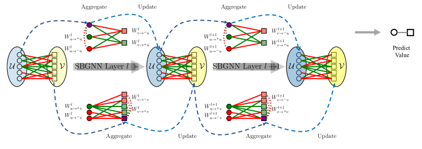
Figure 3. Illustration of SBGNN. SBGNN Layer includes Aggeregate and Update functions. The aggregated message comes from the Set₁ and Set₂ with positive and negative links. After getting the embedding of the node $u_{i}$ and $v_{i}$, it can be used to predict the link sign relationship.

5.1. Message and Aggregation Function

As we discussed in Section 3, comparing to traditional unsigned networks, the links in signed bipartite networks is cross-set and complex (e.g., $u\rightarrow^{+/-}v$).

The message function of vanilla GNNs cannot be directly applied to signed bipartite networks. As shown in Figure 3, we design a new message function to aggregate messages from different sets of neighborhoods . We define that Set₁ refers to the set of node with different types, and Set₂ refers to the set of nodes with the same types. Message from Set₁ and Set₂ can be viewed as the modeling of Perspective 1 and Perspective 2 in Section 3, respectively.

5.1.1. Message from Set₁

For Set₁, the type of the set is different from the type of the current node, and because it is a signed network, its links include both positive and negative relationships. Neighborhood nodes under positive and negative links have different semantic relations. So we use $W_{v\rightarrow^{+}u}$ and $W_{v\rightarrow^{-}u}$ to aggregate the message from $v$ to $u$ with positive and negative links and $W_{u\rightarrow^{+}v}$ and $W_{u\rightarrow^{-}v}$ to aggregate the message from $u$ to $v$ with positive and negative links. For example, in Figure 3, for the purple circle $u_{1}$, the red square $v_{2}$ and the green square $v_{4}$ are the positive and negative neighborhoods, respectively.

At SBGNN Layer $l$-th layer, we use $W^{l}_{v\rightarrow^{+}u},W^{l}_{v\rightarrow^{-}u}$ to collect the message from $v_{j}$ to $u_{i}$ by

(2) $$m^{l}_{v\rightarrow^{+}u}(v_{j},u_{i}) =\textsc{Msg}(h^{l}_{u_{i}},h^{l}_{v_{j}})=W^{l}_{v\rightarrow^{+}u}\cdot h^{l}_{v_{j}},v_{j}\in\mathcal{N}_{v\rightarrow^{+}u}({u_{i}}),$$

$$m^{l}_{v\rightarrow^{-}u}(v_{j},u_{i}) =\textsc{Msg}(h^{l}_{u_{i}},h^{l}_{v_{j}})=W^{l}_{v\rightarrow^{-}u}\cdot h^{l}_{v_{j}},v_{j}\in\mathcal{N}_{v\rightarrow^{-}u}({u_{i}}).$$

where $\mathcal{N}_{v\rightarrow^{+}u}(u_{i})$ and $\mathcal{N}_{v\rightarrow^{-}u}(u_{i})$ are the neighborhood with positive and negative links to $u_{i}$. Similarly, we use we use $W^{l}_{u\rightarrow^{+}v},W^{l}_{u\rightarrow^{-}v}$ to collect the message from Set₁ for $v_{i}$:

(3) $$m^{l}_{u\rightarrow^{+}v}(u_{j},v_{i}) =\textsc{Msg}(h^{l}_{v_{i}},h^{l}_{u_{j}})=W^{l}_{u\rightarrow^{+}v}\cdot h^{l}_{u_{j}},u_{j}\in\mathcal{N}_{u\rightarrow^{+}v}(v_{i}),$$

$$m^{l}_{u\rightarrow^{-}v}(u_{j},v_{i}) =\textsc{Msg}(h^{l}_{v_{i}},h^{l}_{u_{j}})=W^{l}_{u\rightarrow^{+}v}\cdot h^{l}_{u_{j}},u_{j}\in\mathcal{N}_{u\rightarrow^{-}v}(v_{i}).$$

where $\mathcal{N}_{u\rightarrow^{+}v}(v_{i})$ and $\mathcal{N}_{u\rightarrow^{-}v}(v_{i})$ are the neighborhood with positive and negative links to $v_{i}$.

5.1.2. Message from Set₂

As we said before, Set₂ is the node set of the same type. However, there are no links between nodes of the same type, so we need to construct an sign link between nodes of the same type through sign construction in Section 3.

After sign construction, we can aggregate message for the positive and negative links from $u_{j}$ to $u_{i}$ with $W_{u\rightarrow^{+}u}$ and $W_{u\rightarrow^{-}u}$, respectively and $v_{j}$ to $v_{i}$ with $W_{v\rightarrow^{+}v}$ and $W_{v\rightarrow^{-}v}$, respectively.

In Figure 3, for the purple circle $u_{1}$, the green circle $u_{3}$ and the red circle $u_{5}$ are the positive and negative neighborhoods because of the link $u_{1}\rightarrow^{-}v_{2}\rightarrow^{-}u_{3}$ and $u_{1}\rightarrow^{-}v_{2}\rightarrow^{+}u_{5}$. For the purple square $v_{5}$, $v_{1}$ and $v_{2}$ are the negative neighborhoods, $v_{3}$ and $v_{4}$ are the positive neighborhoods based on our sign construction.

In summary, we can definite the message from Set₂ as follows:

(4) $$m^{l}_{u\rightarrow^{+}u}(u_{j},u_{i}) =\textsc{Msg}(h^{l}_{u_{i}},h^{l}_{u_{j}})=W^{l}_{u\rightarrow^{+}u}\cdot h^{l}_{u_{j}},u_{j}\in\mathcal{N}_{u\rightarrow^{+}u}(u_{i}),$$

$$m^{l}_{u\rightarrow^{-}u}(u_{j},u_{i}) =\textsc{Msg}(h^{l}_{u_{i}},h^{l}_{u_{j}})=W^{l}_{u\rightarrow^{-}u}\cdot h^{l}_{u_{j}},u_{j}\in\mathcal{N}_{u\rightarrow^{-}u}(u_{i}),$$

$$m^{l}_{v\rightarrow^{+}v}(v_{j},v_{i}) =\textsc{Msg}(h^{l}_{v_{i}},h^{l}_{v_{j}})=W^{l}_{v\rightarrow^{+}v}\cdot h^{l}_{v_{j}},v_{j}\in\mathcal{N}_{v\rightarrow^{+}v}(v_{i}),$$

$$m^{l}_{v\rightarrow^{-}v}(v_{j},v_{i}) =\textsc{Msg}(h^{l}_{v_{i}},h^{l}_{v_{j}})=W^{l}_{v\rightarrow^{-}v}\cdot h^{l}_{v_{j}},v_{j}\in\mathcal{N}_{v\rightarrow^{-}v}(v_{i}),$$

where $\mathcal{N}_{u\rightarrow^{-}u}(u_{i})$, $\mathcal{N}_{u\rightarrow^{-}u}(u_{i})$, $\mathcal{N}_{v\rightarrow^{+}v}(v_{i})$, and $\mathcal{N}_{v\rightarrow^{-}v}(v_{i})$ are positive and negative neighborhoods for $u_{i}$ and $v_{i}$, respectively.

5.1.3. Aggregation Design

For message aggregation, it is commonly a differentiable, permutation invariant set function (e.g., mean, max, and sum) that take a countable message set $\{m_{v}(u_{i})|u_{i}\in\mathcal{N}(v)\}$ as input; and output a message vector $m_{v}$. In this paper, we use mean (Mean) and graph attention (Gat) aggregation functions.

For the Mean aggregation function, we get $m^{l}(u_{i})$ and $m^{l}(v_{i})$ by Mean the message of neighborhoods:

(5) $$m_{{\leadsto}u}^{l}(u_{i}) =\textsc{Mean}(\{m^{l}_{\leadsto u}(j),\forall j\in\mathcal{N}_{\leadsto u}(u_{i})\}),$$

$$m_{{\leadsto}v}^{l}(v_{i}) =\textsc{Mean}(\{m^{l}_{\leadsto v}(j),\forall j\in\mathcal{N}_{\leadsto v}(v_{i})\})$$

where $\leadsto u$ is a relationship of links to $u$ (e.g., , $v\rightarrow^{+}u$) and $\leadsto v$ is a relationship of links to $v$ (e.g., , $u\rightarrow^{+}v$).

For a graph attention function, it will firstly compute $\alpha^{ij}_{\leadsto}$ for node $i$ and node $j$ by the attention mechanism $\vec{\bf a}_{\leadsto}$ and LeakyReLU nonlinearity activation function (with negative input slope $\alpha$ = 0.2) as:

(6) $$\alpha^{ij}_{\leadsto}=\frac{\exp\left(\text{LeakyReLU}\left(\vec{\bf a}_{\leadsto}^{\top}\cdot[{\bf W}^{l}_{\leadsto}{h^{l}_{i}}\|{\bf W}^{l}_{\leadsto}{h^{l}_{j}}]\right)\right)}{\sum_{k\in\mathcal{N}_{\leadsto}(i)}\exp\left(\text{LeakyReLU}\left(\vec{\bf a}_{\leadsto}^{\top}\cdot[{\bf W}^{l}_{\leadsto}{h^{l}_{i}}\|{\bf W}^{l}_{\leadsto}{h^{l}_{k}}]\right)\right)},$$

where $\|$ is is the concatenation operation, $\cdot^{\top}$ represents transposition, $\mathcal{N}_{\leadsto}(i)$ is the neighborhoods of node $i$ under the definition of $\leadsto$ (e.g., , $u\rightarrow^{+}v$) , ${\bf W}^{l}$ is the weight matrix parameter. Then we can compute $m^{l}(u_{i})$ and $m^{l}(v_{i})$ with $\alpha_{\leadsto}$:

(7) $$m_{{\leadsto}u}^{l}(u_{i}) =\sum_{j\in\mathcal{N}_{\leadsto u}(u_{i})}\alpha^{u_{i}j}_{\leadsto u}\cdot m^{l}_{\leadsto u}(j),$$

$$m_{{\leadsto}v}^{l}(v_{i}) =\sum_{j\in\mathcal{N}_{\leadsto v}(v_{i})}\alpha^{v_{i}j}_{\leadsto v}\cdot m^{l}_{\leadsto v}(j),$$

where $\leadsto u$ is a relationship of links to $u$ (e.g., , $v\rightarrow^{+}u$) and $\leadsto v$ is a relationship of links to $v$ (e.g., , $u\rightarrow^{+}v$). The attention aggregation can be seen as a learnable weighted average function.

5.2. Update Function

For our vertex update function, we concatenate the messages from different neighborhoods with origin node features and apply it to an Mlp to get the final node representation:

(8) $$h^{l+1}_{u} =\textsc{Mlp}(h^{l}_{u}~{}\|~{}m^{l}_{v\rightarrow^{+}u}~{}\|~{}m^{l}_{v\rightarrow^{-}u}~{}\|~{}m^{l}_{u\rightarrow^{+}u}~{}\|~{}m^{l}_{u\rightarrow^{-}u}),$$

$$h^{l+1}_{v} =\textsc{Mlp}(h^{l}_{v}~{}\|~{}m^{l}_{u\rightarrow^{+}v}~{}\|~{}m^{l}_{u\rightarrow^{-}v}~{}\|~{}m^{l}_{v\rightarrow^{+}v}~{}\|~{}m^{l}_{v\rightarrow^{-}v}),$$

where $\|$ is the concatenation operation. More specificlly, the Mlpis a two-layer neural networks with Dropout layer and Act activation function:

(9) $$\textsc{Mlp}(x)=W_{2}\Big{(}\textsc{Act}\big{(}\textsc{Dropout}(W_{1}x+b_{1})\big{)}\Big{)}+b_{2},$$

where $W_{1},b_{1}$ and $W_{2},b_{2}$ is the parameters for this MLP, and Dropout is the dropout function ($p=0.5$ in this paper) and Act is the activation function (e.g., $\mathrm{PReLU}$ (He et al., 2015) in this paper) .

5.3. Loss Function

After getting embeddings $z_{u_{i}}\in\mathbb{R}^{d_{u}}$ and $z_{v_{j}}\in\mathbb{R}^{d_{v}}$ of the node $u_{i}$ and $v_{j}$, we can use following methods to get the prediction value for $u_{i}\rightarrow v_{j}$. The first one is the product operation:

(10) $$y_{pred}=\mathrm{sigmoid}(z_{u_{i}}^{\top}\cdot z_{v_{j}}),$$

where $\cdot^{\top}$ is the transpose function and $\mathrm{sigmoid}$ is the sigmoid function $f(x)=\frac{1}{1+e^{-x}}$. This method should keep the embedding dimension the same (i.e., $d_{u}=d_{v}$). Another method is to use an Mlp to predict the values by

(11) $$y_{pred}=\mathrm{sigmoid}\big{(}\textsc{Mlp}(z_{u_{i}}~{}\|~{}z_{v_{i}})\big{)}$$

where Mlp is a two layer neural networks, $\|$ is the concatenation operation. The Mlp can be viewd as the Edge Learner in (Agrawal and de Alfaro, 2019).

After getting the prediction values, we use binary cross entropy as the loss function:

(12) $$\quad\mathcal{L}=-w\left[y\cdot\log y_{pred}+(1-y)\cdot\log(1-y_{pred})\right]$$

where $w$ is the rescaling weight for the unblanced negative ratios (It is the weights inversely proportional to class frequencies in the input data); $y$ is the ground truth with mapping $\{-1,1\}$ to $\{0,1\}$.

5.4. Training SBGNN

With the design of our SBGNN model, the training procedure is summarized in Algorithm 1.

0:   Signed Bipartite Graph $\mathcal{G}(\mathcal{U},\mathcal{V},\mathcal{E})$;

Encoder Aggregators $Enc$;

SBGNN Layer Number $L$;

Epoch $T$;

0:   Node representation $Z_{\mathcal{U}},Z_{\mathcal{V}}$

1:  Prepare original node embeddings $z^{0}_{u},z^{0}_{v},\forall u\in\mathcal{U},\forall v\in\mathcal{V}$.

2:  Initialize the parameters of SBGNN model.

3:  for $epoch=1,...,T$ do

4:     Get neighborhoods $\mathcal{N}_{v\rightarrow^{+}u}(u_{i})$, $\mathcal{N}_{v\rightarrow^{-}u}(u_{i})$, $\mathcal{N}_{u\rightarrow^{+}u}(u_{i})$, $\mathcal{N}_{u\rightarrow^{-}u}(u_{i})$, $\forall u_{i}\in\mathcal{U}$

5:     Get neighborhoods $\mathcal{N}_{u\rightarrow^{+}v}(v_{i})$, $\mathcal{N}_{u\rightarrow^{-}v}(v_{i})$, $\mathcal{N}_{v\rightarrow^{+}v}(v_{i})$, $\mathcal{N}_{v\rightarrow^{-}v}(v_{i})$, $\forall v_{i}\in\mathcal{V}$

6:     for $l=0...L-1$ do

7:         $z_{u_{i}}^{l+1}\leftarrow Enc^{l}\Big{(}h^{l}_{u_{i}},m^{l}_{v\rightarrow^{+}u}(u_{i}),m^{l}_{v\rightarrow^{-}u}(u_{i})$,

$m^{l}_{u\rightarrow^{+}u}(u_{i}),m^{l}_{u\rightarrow^{-}u}(u_{i})\Big{)}$, $\forall u_{i}\in\mathcal{U}$

8:         $z_{v_{i}}^{l+1}\leftarrow Enc^{l}\Big{(}h^{l}_{v_{i}},m^{l}_{u\rightarrow^{+}v}({v_{i}}),m^{l}_{u\rightarrow^{-}v}({v_{i}})$,

$m^{l}_{v\rightarrow^{+}v}({v_{i}}),m^{l}_{v\rightarrow^{-}v}({v_{i}})\Big{)}$, $\forall v_{i}\in\mathcal{V}$

9:     end for

10:     Compute loss $\sum\limits_{u\rightarrow v\in\mathcal{E}}\mathcal{L}_{loss}(u\rightarrow v)$ with $Z_{\mathcal{U}}$ and $Z_{\mathcal{V}}$

11:     Back propagation, update parameters.

12:  end for

13:  return  $Z^{l}_{\mathcal{U}},Z^{l}_{\mathcal{V}}$

Algorithm 1 SBGNN Algorithm

Algorithm 1 demonstrates that our SBGNN is a layer-by-layer architecture design, where $Enc$ can be any powerful GNN aggregators like Mean or Gat.

6. Experiments

In this section, we evaluate the performance of our proposed SBGNN on real-world datasets. We first introduce the datasets, baselines, and metrics for experiments, then present the experimental results of SBGNN and baselines. Finally, we analyze our models from parameter analysis and ablation study.

6.1. Experimental Settings

6.1.1. Datasets

As previously discussed in Section 3.1, we choose four datasets for this study, namely, Bonanza, U.S. House, U.S. Senate, and Review (we use Final Review as the Review dataset). Following the experimental settings in (Derr et al., 2019), we randomly select 10% of the links as test set, utilize a random 5% for validation set, and the remaining 85% as training set for each of our datasets. We run with different train-val-test splits for 5 times to get the average scores.

6.1.2. Competitors

We compare our method SBGNN with several baselines including Random Embeddings, Unsigned Network Embeddings, Signed/Bipartite Network Embeddings, and Signed Butterfly Based Methods as follows.

Random Embeddings: It generates $d$ dimensional random values from a uniform distribution over $[0,1)$ (i.e., $z=(z_{1},z_{2},...,z_{d})$, $z_{i}\in[0,1)$). Given embeddings $z_{u_{i}}$ and $z_{v_{j}}$, we concatenate them and use a Logistic Regression (Lr) to predict the value of $u_{i}$ and $v_{i}$. Lr will be trained on the training set, and make predictions on the test set. Since Lr has learnable parameters, this method can be viewed as the lower bound of the graph representation learning methods.

Unsigned Network Embeddings: Comparing random embeddings, we use some classical unsigned network embedding methods (e.g., DeepWalk (Perozzi et al., 2014), Node2vec (Grover and Leskovec, 2016), LINE (Tang et al., 2015)). By keeping only positive links, we input unsigned networks to such unsigned network embedding methods to get embeddings for $u_{i}$ and $v_{j}$. As same as Random Embeddings, we concatenate embeddings $z_{u_{i}}$ and $z_{v_{j}}$, and use Lr to predict the sign of links.

Signed/Bipartite Network Embedding: We use Signed or/and Bipartite Network Embedding as our baselines. More specifically, we use SiNE (Wang et al., 2017) to learn the embeddings for $u_{i}$ and $v_{i}$ after sign link construction in Section 3. For BiNE (Gao et al., 2018), we remove the negative links between $\mathcal{U}$ and $\mathcal{V}$ . We use BiNE to get embeddings $z_{u_{i}}$ and $z_{v_{j}}$ and use Lr to predict the sign of links with concatenating $z_{u_{i}}$ and $z_{v_{j}}$. Compared with the unsigned network embeddings methods, we try to let the representation learn the structural information (e.g., links between $\mathcal{U}$ and $\mathcal{V}$ and the link sign) instead of just relying on the downstream classifier. SBiNE (Zhang et al., 2020) is a representation learning method for signed bipartite networks, which preserves the first-order and second-order proximity. Instead of a two-stage model, SBiNE uses single neural networks with sigmoid nonlinearity function to predict the value of $u_{i}$ and $v_{j}$.

Signed Butterfly Based Methods: Based on the analysis of signed butterfly isomorphism, (Derr et al., 2019) proposes a variety of methods for  Link Sign Prediction , including SCsc, MFwBT, and SBRW . Specifically, SCsc is a balance theory guided feature extraction method. MFwBT is the matrix factorization model with balance theory. SBRW is the signed bipartitle random walk method. Due to the findings about receiving aid in prediction from balance theory will always perform better than the methods that only use generic signed network information  (Derr et al., 2019), we take the SCsc as the most competitive baseline for our SBGNN model.

Signed Bipartite Graph Neural Networks: For our SBGNN, we try two different aggregation design (i.e., Mean and Gat) and remark it as SBGNN-Mean and SBGNN-Gat, respectively.

For a fair comparison, we set all the node embedding dimension to 32 which is as same as that in SBiNE (Zhang et al., 2020) for all embedding based methods. For other parameters in baselines, we follow the recommended settings in their original papers. For embedding methods, we use the balanced class weighted Logistic Regression in Scikit-learn (Pedregosa et al., 2011). For SBiNE, we use PyTorch (Paszke et al., 2019) to implement it by ourselves. For our SBGNN, we also use PyTorch to implement our model. We use Adam optimizer with an initial learning rate of 0.005 and a weight decay of 1e-5. We run 2000 epochs for SBGNN and choose the model that performs the best AUC metrics on the validation set.

6.1.3. Evaluation Metrics

Since  Link Sign Prediction is a binary classification problem, we use AUC, Binary-F1, Macro-F1, and Micro-F1 to evaluate the results. These metrics are widely used in  Link Sign Prediction  (Chen et al., 2018; Huang et al., 2021b). Note that, among all these four evaluation metrics, the greater the value is, indicating the better the performance of the corresponding method.

6.2. Experiment Results

Table 3. The results of  Link Sign Prediction on four datasets. Results not available are marked as ‘#N/A’. Two-tailed t-tests demonstrate the improvements of our SBGNN to the baseline SCsc are statistically significant ( ^∗ indicates p-value $\leq$ 0.05).

		Random Embedding	Unsigned Network Embedding			Signed/Bipartite Network Embedding			Signed Butterfly Based Methods			Signed Bipartite Graph Neural Networks
Dataset	Metric	Random	Deepwalk	Node2vec	LINE	SiNE	BiNE	SBiNE	SCsc	MFwBT	SBRW	SBGNN-Mean	SBGNN-Gat
Bonanza	AUC	0.5222	0.6176	0.6185	0.6124	0.6088	0.6026	0.5525	0.6524	0.5769	0.5315	0.5841	0.5769
	Binary-F1	0.7282	0.7843	0.7530	0.6974	0.9557	0.7426	0.8514	0.6439	0.8927	0.9823	0.9488∗	0.9616∗
	Macro-F1	0.3868	0.4258	0.4087	0.3790	0.5422	0.4016	0.4538	0.3543	0.4813	0.5353	0.5311∗	0.5404∗
	Micro-F1	0.5770	0.6497	0.6093	0.5424	0.9157	0.5960	0.7436	0.4843	0.8076	0.9652	0.9044∗	0.9269∗
Review	AUC	0.5489	0.6324	0.6472	0.6236	0.5741	#N/A	0.5329	0.5522	0.4727	0.5837	0.6584∗	0.6747∗
	Binary-F1	0.4996	0.5932	0.6141	0.5974	0.5247	#N/A	0.4232	0.3361	0.4346	0.5423	0.6128∗	0.6366∗
	Macro-F1	0.5426	0.6268	0.6400	0.6120	0.5688	#N/A	0.5262	0.4823	0.4696	0.5767	0.6556∗	0.6629∗
	Micro-F1	0.5487	0.6325	0.6444	0.6137	0.5744	#N/A	0.5521	0.5812	0.4752	0.5812	0.6632∗	0.6667∗
U.S. House	AUC	0.5245	0.6223	0.6168	0.5892	0.6006	0.6103	0.8328	0.8274	0.8097	0.8224	0.8474∗	0.8481∗
	Binary-F1	0.5431	0.6401	0.6323	0.6304	0.6118	0.6068	0.8434	0.8375	0.8234	0.8335	0.8549∗	0.8560∗
	Macro-F1	0.5238	0.6215	0.6158	0.5883	0.5991	0.6097	0.8323	0.8267	0.8096	0.8219	0.8463∗	0.8471∗
	Micro-F1	0.5246	0.6224	0.6166	0.5892	0.5996	0.6108	0.8330	0.8274	0.8106	0.8226	0.8468∗	0.8476∗
U.S. Senate	AUC	0.5251	0.6334	0.6260	0.5743	0.5875	0.6071	0.7998	0.8163	0.7857	0.8142	0.8209∗	0.8246∗
	Binary-F1	0.5502	0.6603	0.6526	0.6159	0.5923	0.5968	0.8175	0.8294	0.8043	0.8291	0.8277	0.8320
	Macro-F1	0.5239	0.6325	0.6251	0.5722	0.5842	0.6037	0.7992	0.8148	0.7850	0.8131	0.8177∗	0.8215∗
	Micro-F1	0.5254	0.6347	0.6271	0.5732	0.5848	0.6042	0.8009	0.8160	0.7867	0.8145	0.8183∗	0.8221∗

We show the results in Table 3. We have bolded the highest value of each row and underlined the second value. From Table 3, we make the following observations:

• Even with random embedding, Lr can still achieve a certain effect on  Link Sign Prediction (i.e., AUC ¿ 0.5).

  It demonstrates that the downstream classifier has a certain predictive ability for  Link Sign Prediction when it is regarded as a two-stage model.

• After using network embeddings, the graph structure data is modeled into the node representation, which improves the prediction results. Even the worst-performing LINE outperforms random embedding by 17.3%, 13.6%, 12.3%, and 9.4% on AUC in Bonanza, Review, U.S. House, and U.S. Senate, respectively. It demonstrate that graph structure information is helpful for  Link Sign Prediction . In unsigned network embedding methods, Node2vec has made the best results in the unsigned network embeddings methods. We guess that the biased random walk mechanism may be able to explore the graph structure more effectively.

• For signed or bipartite model (i.e., SiNE and BiNE), the information for sign and bipartite network structure can contribute to the node representation learning. SiNE is more effective than BiNE (e.g., AUC in Bonanza (0.6088 ¿ 0.6026)), indicating that link sign information may be more important than the link relationship. The performance of SBiNE is not as good as that in (Zhang et al., 2020). This can be due to the fact of different data splits and implementation details.

• The signed butterfly based methods (i.e., SCsc, MFwBT, and SBRW) outperform Deepwalk by 33.0%, 30.1%, and 32.2% on AUC in U.S. House, achieve 28.9%, 24.3% and 28.5% gains on AUC in U.S. Senate, respectively. It shows that modeling the balance theory in the signed bipartite network is key for  Link Sign Prediction . But in Review and Bonanza datasets, the signed butterfly based methods cannot outperform embedding based methods. This can be due to that there are fewer signed butterfly isomorphism in these two datasets. Besides, Bonanza is an extremely unbalanced dataset (i.e., % Positive Links is 0.980), AUC and F1 show a big difference.

• Our SBGNN model achieve the best results on most metrics. Except bonanza, SBGNN-Mean and SBGNN-Gat significantly outperform SCsc. In bonanza, SBGNN-Gat significantly gains better results in Binary-F1, Macro-F1, and Micro-F1. It demonstrates that SBGNN effectively models signed bipartite networks. Besides, we can find that Gat aggregator is better than Mean aggregator, which can be attributed to the attention mechanism (Vaswani et al., 2017).

6.3. Parameter Analysis and Ablation Study

In this subsection, we conduct parameter analysis and ablation study for our SBGNN model. We choose the U.S. House as our dataset and select 85% training edges, 5% validation edges, and 15% test edges as before.

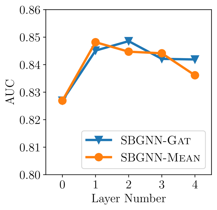
(a) #Layer $l$

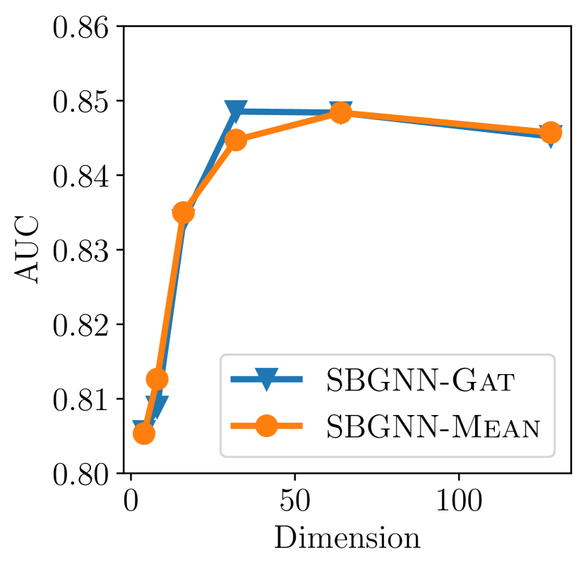
(b) Dimension $d$

Figure 4. Parameter analysis on the number of SBGNN Layer $l$ and imension $d$ for SBGNN on the U.S. House dataset.

6.3.1. Parameter Analysis

We analyze the number of our SBGNN Layer $l$ and the dimension $d$ of embeddings. For the number of our SBGNN Layer $l$, we vary $l$ from $\{0,1,2,3,4\}$. Note that, $l=0$ means there is no GNN Layer is used (i.e., just lookup embeddings is used), so the results for SBGNN-Mean and SBGNN-Gat are same. For Figure 4(a), we can find that GNN Layer is more effective than the lookup embedding methods. For SBGNN-Mean, the best $l$ is 1, which AUC is 0.8481. But for SBGNN-Gat, two SBGNN Layers will get a better results. For the dimension of SBGNN, we choose the value $d$ from $\{4,8,16$, $32,64,128\}$ to analyze the effects of dimensions. From Figure 4(b), we can find that as the value increases from 4 to 32, AUC on SBGNN-Gat increases from 0.8056 to 0.8485; AUC on SBGNN-Mean increases from 0.8053 to 0.8447. After 32 for SBGNN-Mean and 64 for SBGNN-Gat, the AUC value slightly descrease. This result can be due to the reason that large dimension $d$ will cause the difficulties of training embeddings.

Table 4. Ablation study results for SBGNN model on the U.S. House dataset.

Method	AUC	Binary-F1	Macro-F1	Micro-F1
SBGNN-Gat	0.8485	0.8586	0.8477	0.8485
SBGNN-Gat (w/o Set1)	0.8406	0.8521	0.8400	0.8409
SBGNN-Gat (w/o Set2)	0.8440	0.8567	0.8438	0.8448
SBGNN-Gat (with Lr)	0.6281	0.6195	0.6227	0.6227
SBGNN-Gat (with Mlp)	0.8365	0.8480	0.8358	0.8367
SBGNN-Mean	0.8447	0.8519	0.8429	0.8434
SBGNN-Mean (w/o Set1)	0.8419	0.8496	0.8402	0.8408
SBGNN-Mean (w/o Set2)	0.8296	0.8410	0.8288	0.8297
SBGNN-Mean (with Lr)	0.6285	0.6387	0.6263	0.6267
SBGNN-Mean (with Mlp)	0.8443	0.8531	0.8430	0.8436

6.3.2. Ablation Study

For the ablation study, we investigate the effect of different aggregation and prediction functions. Firstly, as we discussed in Section 6.2, Gat aggregator is better than Mean aggregators. We further investigate the effect for our message function design. From Table 4, we can see that without message from Set₁ (i.e., w/o Set₁), SBGNN-Gat and SBGNN-Mean descrease 0.9% and 0.3%, respectively; without Set₂ message (i.e., w/o Set₂), SBGNN-Gat and SBGNN-Mean descrease 0.5% and 1.8%, respectively. It demonstrates that both message from Set₁ and Set₁ is useful for the SBGNN model. As we discussed in Section 5.3, the prediction can be achieved by product operation or Mlp. We replace it with a simple Lr layer or a two-layer Mlp. From Table 4, we can find that Mlp is much better than simple Lr but not better than product operation.

7. Conclusions and Future Work

In this paper, we focus on modeling signed bipartite networks. We first discuss two different perspectives to model the signed bipartite networks. Through sign construction, the new perspective can count the signed triangles in the same node type networks. It obtains consistent results with signed butterfly analysis. We further use these two perspectives to model peer review and find that after rebuttal, the balance of reviewers’ opinions improved. It shows that the rebuttal mechanism makes the reviewer’s opinions more consistent. Under the definition of a new perspective, we propose a new graph neural network model SBGNN to learn the node representation of signed bipartite graphs. On four real-world datasets, our method has achieved state-of-the-art results. Finally, we conducted parameter analysis and ablation study on SBGNN.

In future work, we will explore signed bipartite networks with node features, which can improve the  Link Sign Prediction  (Karimi et al., 2019) and node classification (Tang et al., 2016a). For example, in the prediction of bill vote, if the node features can be modeled, such as the political standpoint of the congress, it will be more effective in predicting the vote results. Besides, we will also try to introduce signed bipartite graph neural networks into recommender system (Tang et al., 2016b).

- (1)
- Agrawal and de Alfaro (2019) Rakshit Agrawal and Luca de Alfaro. 2019. Learning Edge Properties in Graphs from Path Aggregations. In The World Wide Web Conference (San Francisco, CA, USA) (WWW ’19). Association for Computing Machinery, New York, NY, USA, 15–25. https://doi.org/10.1145/3308558.3313695
- Bonchi et al. (2019) Francesco Bonchi, Edoardo Galimberti, Aristides Gionis, Bruno Ordozgoiti, and Giancarlo Ruffo. 2019. Discovering polarized communities in signed networks. In Proceedings of the 28th ACM International Conference on Information and Knowledge Management. 961–970.
- Cartwright and Harary (1956) Dorwin Cartwright and Frank Harary. 1956. Structural balance: a generalization of Heider’s theory. Psychological review 63, 5 (1956), 277.
- Chen et al. (2018) Yiqi Chen, Tieyun Qian, Huan Liu, and Ke Sun. 2018. “Bridge” Enhanced Signed Directed Network Embedding. In Proceedings of the 27th ACM International Conference on Information and Knowledge Management. 773–782.
- Derr et al. (2019) Tyler Derr, Cassidy Johnson, Yi Chang, and Jiliang Tang. 2019. Balance in signed bipartite networks. In Proceedings of the 28th ACM International Conference on Information and Knowledge Management. 1221–1230.
- Derr et al. (2018) Tyler Derr, Yao Ma, and Jiliang Tang. 2018. Signed graph convolutional networks. In 2018 IEEE International Conference on Data Mining (ICDM). IEEE, 929–934.
- Derr et al. (2020) Tyler Derr, Zhiwei Wang, Jamell Dacon, and Jiliang Tang. 2020. Link and interaction polarity predictions in signed networks. Social Network Analysis and Mining 10, 1 (2020), 1–14.
- Easley and Kleinberg (2010) David Easley and Jon Kleinberg. 2010. Networks, crowds, and markets: Reasoning about a highly connected world. Vol. 8. Cambridge University Press.
- Facchetti et al. (2011) Giuseppe Facchetti, Giovanni Iacono, and Claudio Altafini. 2011. Computing global structural balance in large-scale signed social networks. Proceedings of the National Academy of Sciences 108, 52 (2011), 20953–20958.
- Gao et al. (2018) Ming Gao, Leihui Chen, Xiangnan He, and Aoying Zhou. 2018. Bine: Bipartite network embedding. In The 41st international ACM SIGIR conference on research & development in information retrieval. 715–724.
- Gilmer et al. (2017) Justin Gilmer, Samuel S Schoenholz, Patrick F Riley, Oriol Vinyals, and George E Dahl. 2017. Neural message passing for quantum chemistry. In International Conference on Machine Learning. PMLR, 1263–1272.
- Grover and Leskovec (2016) Aditya Grover and Jure Leskovec. 2016. node2vec: Scalable feature learning for networks. In Proceedings of the 22nd ACM SIGKDD international conference on Knowledge discovery and data mining. 855–864.
- Hamilton et al. (2017a) William L Hamilton, Rex Ying, and Jure Leskovec. 2017a. Inductive representation learning on large graphs. In Proceedings of the 31st International Conference on Neural Information Processing Systems. 1025–1035.
- Hamilton et al. (2017b) William L Hamilton, Rex Ying, and Jure Leskovec. 2017b. Representation learning on graphs: Methods and applications. arXiv preprint arXiv:1709.05584 (2017).
- He et al. (2015) Kaiming He, Xiangyu Zhang, Shaoqing Ren, and Jian Sun. 2015. Delving deep into rectifiers: Surpassing human-level performance on imagenet classification. In Proceedings of the IEEE international conference on computer vision. 1026–1034.
- Heaven (2018) Douglas Heaven. 2018. AI peer reviewers unleashed to ease publishing grind. Nature 563, 7731 (2018), 609–609.
- Heider (1944) Fritz Heider. 1944. Social perception and phenomenal causality. Psychological review 51, 6 (1944), 358.
- Huang et al. (2021a) Junjie Huang, Huawei Shen, and Xueqi Cheng. 2021a. SIGNLENS: A Tool for Analyzing People’s Polarization Social Relationship Based on Signed Graph Modeling. In Proceedings of the International AAAI Conference on Web and Social Media, Vol. 15. 1091–1093.
- Huang et al. (2019) Junjie Huang, Huawei Shen, Liang Hou, and Xueqi Cheng. 2019. Signed graph attention networks. In Proceedings of the International Conference on Artificial Neural Networks. Springer, 566–577.
- Huang et al. (2021b) Junjie Huang, Huawei Shen, Liang Hou, and Xueqi Cheng. 2021b. SDGNN: Learning Node Representation for Signed Directed Networks. In Proceedings of the AAAI Conference on Artificial Intelligence, Vol. 35. 196–203.
- Javari et al. (2020) Amin Javari, Tyler Derr, Pouya Esmailian, Jiliang Tang, and Kevin Chen-Chuan Chang. 2020. Rose: Role-based signed network embedding. In Proceedings of The Web Conference 2020. 2782–2788.
- Karimi et al. (2019) Hamid Karimi, Tyler Derr, Aaron Brookhouse, and Jiliang Tang. 2019. Multi-factor congressional vote prediction. In Proceedings of the 2019 IEEE/ACM International Conference on Advances in Social Networks Analysis and Mining. 266–273.
- Kipf and Welling (2019) Thomas N Kipf and Max Welling. 2019. Semi-supervised classification with graph convolutional networks. In International Conference on Learning Representations.
- Kirkley et al. (2019) Alec Kirkley, George T Cantwell, and MEJ Newman. 2019. Balance in signed networks. Physical Review E 99, 1 (2019), 012320.
- Leskovec et al. (2010a) Jure Leskovec, Daniel Huttenlocher, and Jon Kleinberg. 2010a. Predicting positive and negative links in online social networks. In Proceedings of the 19th international conference on World wide web. 641–650.
- Leskovec et al. (2010b) Jure Leskovec, Daniel Huttenlocher, and Jon Kleinberg. 2010b. Signed networks in social media. In Proceedings of the SIGCHI conference on human factors in computing systems. 1361–1370.
- Li et al. (2020) Guohao Li, Chenxin Xiong, Ali Thabet, and Bernard Ghanem. 2020. Deepergcn: All you need to train deeper gcns. arXiv preprint arXiv:2006.07739 (2020).
- Li et al. (2018) Yuemeng Li, Shuhan Yuan, Xintao Wu, and Aidong Lu. 2018. On spectral analysis of directed signed graphs. International Journal of Data Science and Analytics 6, 2 (2018), 147–162.
- Mara et al. (2020) Alexandru Mara, Yoosof Mashayekhi, Jefrey Lijffijt, and Tijl De Bie. 2020. CSNE: Conditional Signed Network Embedding. In Proceedings of the 29th ACM International Conference on Information & Knowledge Management. 1105–1114.
- Ou et al. (2016) Mingdong Ou, Peng Cui, Jian Pei, Ziwei Zhang, and Wenwu Zhu. 2016. Asymmetric transitivity preserving graph embedding. In Proceedings of the 22nd ACM SIGKDD international conference on Knowledge discovery and data mining. 1105–1114.
- Paszke et al. (2019) Adam Paszke, Sam Gross, Francisco Massa, Adam Lerer, James Bradbury, Gregory Chanan, Trevor Killeen, Zeming Lin, Natalia Gimelshein, Luca Antiga, et al. 2019. PyTorch: An Imperative Style, High-Performance Deep Learning Library. Advances in Neural Information Processing Systems 32 (2019), 8026–8037.
- Pedregosa et al. (2011) F. Pedregosa, G. Varoquaux, A. Gramfort, V. Michel, B. Thirion, O. Grisel, M. Blondel, P. Prettenhofer, R. Weiss, V. Dubourg, J. Vanderplas, A. Passos, D. Cournapeau, M. Brucher, M. Perrot, and E. Duchesnay. 2011. Scikit-learn: Machine Learning in Python. Journal of Machine Learning Research 12 (2011), 2825–2830.
- Perozzi et al. (2014) Bryan Perozzi, Rami Al-Rfou, and Steven Skiena. 2014. Deepwalk: Online learning of social representations. In Proceedings of the 20th ACM SIGKDD international conference on Knowledge discovery and data mining. 701–710.
- Sanei-Mehri et al. (2018) Seyed-Vahid Sanei-Mehri, Ahmet Erdem Sariyuce, and Srikanta Tirthapura. 2018. Butterfly counting in bipartite networks. In Proceedings of the 24th ACM SIGKDD International Conference on Knowledge Discovery & Data Mining. 2150–2159.
- Shahriari and Jalili (2014) Moshen Shahriari and Mahdi Jalili. 2014. Ranking nodes in signed social networks. Social network analysis and mining 4, 1 (2014), 172.
- Song and Meyer (2015) Dongjin Song and David A Meyer. 2015. Link sign prediction and ranking in signed directed social networks. Social network analysis and mining 5, 1 (2015), 1–14.
- Szell et al. (2010) Michael Szell, Renaud Lambiotte, and Stefan Thurner. 2010. Multirelational organization of large-scale social networks in an online world. Proceedings of the National Academy of Sciences 107, 31 (2010), 13636–13641.
- Tang et al. (2016a) Jiliang Tang, Charu Aggarwal, and Huan Liu. 2016a. Node classification in signed social networks. In Proceedings of the 2016 SIAM international conference on data mining. SIAM, 54–62.
- Tang et al. (2016b) Jiliang Tang, Charu Aggarwal, and Huan Liu. 2016b. Recommendations in signed social networks. In Proceedings of the 25th International Conference on World Wide Web. 31–40.
- Tang et al. (2015) Jian Tang, Meng Qu, Mingzhe Wang, Ming Zhang, Jun Yan, and Qiaozhu Mei. 2015. Line: Large-scale information network embedding. In Proceedings of the 24th international conference on world wide web. 1067–1077.
- Traag and Bruggeman (2009) Vincent A Traag and Jeroen Bruggeman. 2009. Community detection in networks with positive and negative links. Physical Review E 80, 3 (2009), 036115.
- Vaswani et al. (2017) Ashish Vaswani, Noam Shazeer, Niki Parmar, Jakob Uszkoreit, Llion Jones, Aidan N Gomez, Łukasz Kaiser, and Illia Polosukhin. 2017. Attention is All you Need. Advances in Neural Information Processing Systems 30 (2017), 5998–6008.
- Veličković et al. (2018) Petar Veličković, Guillem Cucurull, Arantxa Casanova, Adriana Romero, Pietro Liò, and Yoshua Bengio. 2018. Graph attention networks. International Conference on Learning Representations (2018). https://openreview.net/forum?id=rJXMpikCZ
- Wang et al. (2017) Suhang Wang, Jiliang Tang, Charu Aggarwal, Yi Chang, and Huan Liu. 2017. Signed network embedding in social media. In Proceedings of the 2017 SIAM international conference on data mining. SIAM, 327–335.
- Wu et al. (2020) Zonghan Wu, Shirui Pan, Fengwen Chen, Guodong Long, Chengqi Zhang, and S Yu Philip. 2020. A comprehensive survey on graph neural networks. IEEE Transactions on Neural Networks and Learning Systems (2020).
- Xu et al. (2019) Bingbing Xu, Huawei Shen, Qi Cao, Keting Cen, and Xueqi Cheng. 2019. Graph Convolutional Networks Using Heat Kernel for Semi-Supervised Learning. In Proceedings of the 28th International Joint Conference on Artificial Intelligence (Macao, China) (IJCAI’19). AAAI Press, 1928–1934.
- Xu et al. (2018b) Bingbing Xu, Huawei Shen, Qi Cao, Yunqi Qiu, and Xueqi Cheng. 2018b. Graph Wavelet Neural Network. In International Conference on Learning Representations.
- Xu et al. (2018a) Keyulu Xu, Weihua Hu, Jure Leskovec, and Stefanie Jegelka. 2018a. How Powerful are Graph Neural Networks?. In International Conference on Learning Representations.
- You et al. (2020) Jiaxuan You, Zhitao Ying, and Jure Leskovec. 2020. Design space for graph neural networks. Advances in Neural Information Processing Systems 33 (2020).
- Yuan et al. (2017) Shuhan Yuan, Xintao Wu, and Yang Xiang. 2017. SNE: signed network embedding. In Pacific-Asia conference on knowledge discovery and data mining. Springer, 183–195.
- Zhang et al. (2020) Youwen Zhang, Wei Li, Dengcheng Yan, Yiwen Zhang, and Qiang He. 2020. SBiNE: Signed Bipartite Network Embedding. In International Conference on Collaborative Computing: Networking, Applications and Worksharing. Springer, 479–492.