Quench dynamics and bulk-edge correspondence in nonlinear mechanical systems

Abstract

We study a topological physics in a one-dimensional nonlinear system by taking an instance of a mechanical rotator model with alternating spring constants. This nonlinear model is smoothly connected to an acoustic model described by the Su-Schrieffer-Heeger model in the linear limit. We numerically show that quench dynamics of the kinetic and potential energies for the nonlinear model is well understood in terms of the topological and trivial phases defined in the associated linearized model. It indicates phenomenologically the emergence of the edge state in the topological phase even for the nonlinear system, which may be the bulk-edge correspondence in nonlinear system.

I Introduction

Topological insulatorsHasan ; Qi were originally discovered in in-organic solid state materials. However, it is now well recognized that topological physics is ubiquitous in various systems such as acousticProdan ; TopoAco ; Berto ; Xiao ; He ; Abba ; Xue ; Ni ; Wei ; Xue2 , mechanicalLubensky ; Chen ; Nash ; Paul ; Sus ; Sss ; Huber ; Mee ; Kariyado ; Hannay ; Po ; Rock ; Takahashi ; Mat ; Taka ; Ghatak ; Wakao , photonicKhaniPhoto ; Hafe2 ; Hafezi ; WuHu ; TopoPhoto ; Ozawa ; Hassan ; Li and electric circuitTECNature ; ComPhys ; Hel ; Lu ; YLi ; EzawaTEC ; Research ; Zhao ; EzawaLCR ; EzawaSkin ; Garcia ; Hofmann ; EzawaMajo ; Tjunc ; Lee ; Kot systems. They are called artificial topological systems. The merit of them is that it is possible to fabricate ideal systems comparing to natural solid state materials. Another merit of artificial topological systems is that nonlinearity is naturally introduced into them.

Topological physics is mostly studied in linear systems. There are only a few studies on it in nonlinear systemsKot ; Smi ; Sone ; TopoToda because the study of the topological properties is not straightforward. One of the reasons is that it is a formidable problem to obtain a band structure and a topological number in a generic nonlinear system. Recently, it is proposed to account for the topological properties in nonlinear systems phenomenologically based on the bulk-edge correspondence well established in the linear theoryTopoToda . It seems to work provided that the nonlinear theory is continuously connected to a linear theory where the topological number is well defined. One may say that the topological properties are inherited from a linear theory to a nonlinear theory. It is an interesting problem to explore other systems which share similar properties.

A good signal to detect the topological phase transition is to study quench dynamics starting from one of the edges in the case of one dimension based on the bulk-edge correspondenceQWalk . There is almost no time evolution and the state remains almost localized at the edge for a topological phase. It is because the initial state is almost given by the topological localized edge state, which has no dynamics. On the other hand, the state rapidly spreads into the bulk for a trivial phase because the initial state is composed of bulk eigen functions. Although the usefulness of quench dynamics has been established in a linear system, it is also useful in a nonlinear systemTopoToda .

In this paper, we investigate a one-dimensional mechanical rotator model with alternating spring constants: See Fig.1. It is a nonlinear generalization of the Su-Schrieffer-Heeger (SSH) model. We solve the quench dynamics of a mechanical rotator model as an initial condition problem, where only one rotator at the left-most edge is excited initially. The potential and kinetic energies exhibit distinct behaviors depending on whether the system is in the topological or trivial phase defined in the linearized model. Namely, after enough time, they are well localized in the topological phase, while they are spread over the bulk in the trivial phase. These phenomena are understood in terms of the emergence of the topological edge state in the topological phase. It would represent the bulk-edge correspondence in nonlinear system.

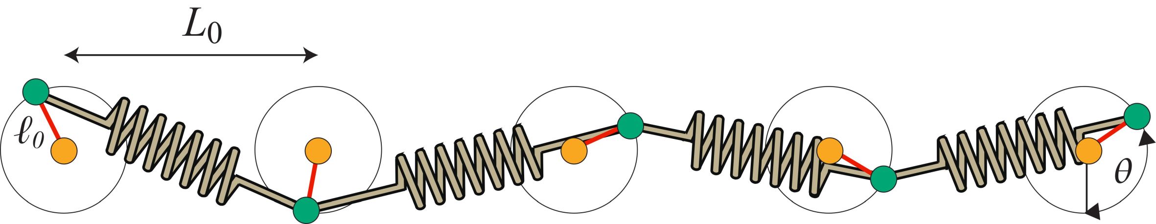
Figure 1: Illustration of the mechanical rotator model. Two adjacent rotators are connected by a spring with the spring constant $\kappa_{j}$. A rotator colored in green rotates around a center colored in orange with the radius $\ell_{0}$. All centers are on a line, and the distance between two adjacent centers is $L_{0}$.

II Mechanical rotator model

We consider a mechanical rotator modelLubensky as illustrated in Fig.1. We place rotators indexed by the number $j$, $j=1,2,\cdots,N$. Each rotator has the radius $\ell_{0}$, and its center is fixed at the position $\left(jL_{0},0\right)$ on the $x$ axis, with $L_{0}$ the distance between two adjacent centers. The dynamical variables are angles $\theta_{j}$ for rotators $j$.

The Hamiltonian of the system consists of the kinetic energy $U^{\text{K}}$, the potential energy of the springs $U^{\text{spring}}$ and the gravitational energy of the $U^{\text{g}}$,

$$H=U^{\text{K}}+U^{\text{spring}}+U^{\text{g}}.$$ (1)

They are given by

$$U^{\text{K}}=\sum_{j}U_{j}^{\text{K}},\quad U_{j}^{\text{K}}=\frac{m}{2}\dot{\theta}_{j}^{2}$$ (2)

with the mass $m$,

$$U^{\text{g}}=-g\sum_{j}\cos\theta_{j}$$ (3)

with the gravitational constant $g$, and

$$U^{\text{spring}} = \sum_{j}U_{j}^{\text{spring}},$$ (4)

$$U_{j}^{\text{spring}} = \frac{1}{2}\kappa_{j}\left(L_{j}\left(\theta_{j},\theta_{j+1}\right)-L\right)^{2},$$ (5)

where $L_{j}\left(\theta_{j},\theta_{j+1}\right)$ is the length of the spring between $j$ and $j+1$ nodes,

$$L_{j}\left(\theta_{j},\theta_{j+1}\right)=\sqrt{\left[L_{j}^{x}\left(\theta_{j},\theta_{j+1}\right)\right]^{2}+\left[L_{j}^{y}\left(\theta_{j},\theta_{j+1}\right)\right]^{2}}$$ (6)

with

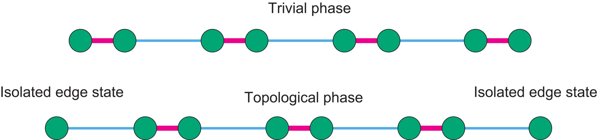
Figure 2: Illustration of the trivial and topological phases in the SSH model. There are two isolated edge states in the topological phase, while all of the sites are dimerized in the trivial phase. Magenta and cyan lines represent strong and weak bondings $\kappa_{j}$ in Eq.(10), respectively. This illustration is argued to hold even in nonlinear system described by Eq.(9).

$$L_{j}^{x}\left(\theta_{j},\theta_{j+1}\right) = \ell_{0}\sin\theta_{j+1}-\ell_{0}\sin\theta_{j}+L_{0},$$ (7)

$$L_{j}^{y}\left(\theta_{j},\theta_{j+1}\right) = \ell_{0}\cos\theta_{j+1}-\ell_{0}\cos\theta_{j}.$$ (8)

The equation of motion is given by

$$m\ddot{\theta}_{j}=-g\sin\theta_{j}-\frac{\partial U^{\text{spring}}}{\partial\theta_{j}}.$$ (9)

The spring constant is assumed to be alternating,

$$\kappa_{j}=\kappa\left(1+\lambda\left(-1\right)^{j}\right),$$ (10)

where the dimerization is controlled by $\lambda$ with $|\lambda|\leq 1$. For $\lambda<0$, the spring constant $\kappa_{j}$ with odd (even) $j$ is strong (weak). On the other hand, for $\lambda>0$, the spring constant $\kappa_{j}$ with odd (even) $j$ is weak (strong): See Fig.2.

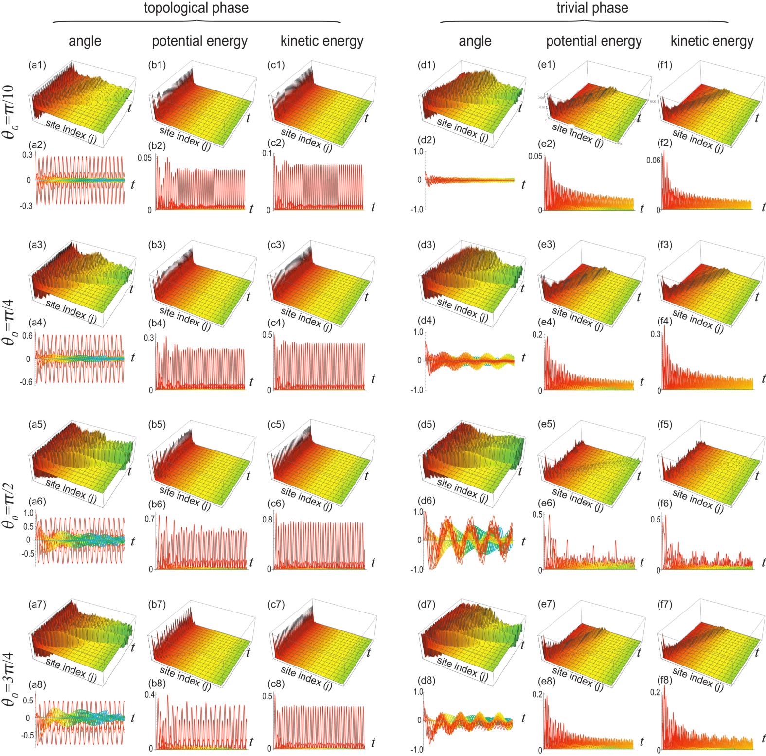
Figure 3: Time evolution of the angle $\sin\theta_{j}$ for (a1)$\sim$(a8) and (d1)$\sim$(d8), the potential energy $U_{j}^{\text{spring}}$ for (b1)$\sim$(b8) and (e1)$\sim$(e8), and the kinetic energy $U_{j}^{\text{K}}$ for (c1)$\sim$(c8) and (f1)$\sim$(f8). (a1)$\sim$(c8) topological phase with $\lambda=-0.5$, and (d1)$\sim$(f8) trivial phase with $\lambda=0.5$. (a1)$\sim$(f2) $\theta_{0}=\pi/10$, (a3)$\sim$(f4) $\theta_{0}=\pi/4$, (a5)$\sim$(f6) $\theta_{0}=\pi/2$, and (a7)$\sim$(f8) $\theta_{0}=3\pi/4$. (a1)$\sim$(f1), (a3)$\sim$(f3), (a5)$\sim$(f5) and (a7)$\sim$(f7) Bird’s eye’s view, and (a2)$\sim$(f2), (a4)$\sim$(f4), (a6)$\sim$(f6) and (a8)$\sim$(f8) Color plot of the time evolution. We have used a chain containing 100 sites. We have set $m=0.01$, $g=0.1$, $L_{0}=10$ and $\ell_{0}=1$. Color indicates the site index $j$, which is manifest in bird’s eye’s views.

III Linearized model

Provided the angle $\theta_{j}$ is small enough, the potential energy is well approximated by the harmonic potential,

$$U^{\text{spring}}=\frac{\ell_{0}^{2}}{2}\sum_{j}\kappa_{j}\left(\theta_{j+1}-\theta_{j}\right)^{2},$$ (11)

and the equation of motion is obtained as

$$m\ddot{\theta}_{j}=-g\theta_{j}-\ell_{0}^{2}\sum_{j}\kappa_{j}\left(\theta_{j}-\theta_{j+1}\right)+\kappa_{j-1}\left(\theta_{j}-\theta_{j-1}\right),$$ (12)

which is a linearized model.

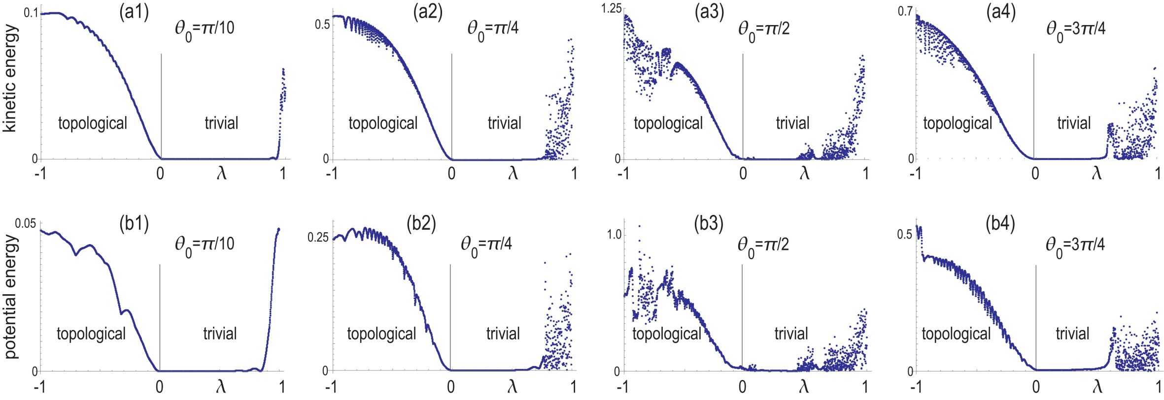
Figure 4: (a1)$\sim$(a4) Kinetic energy at the edge $U_{1}^{\text{K}}$, and (b1)$\sim$(b4) the potential energy at the edge $U_{1}^{\text{spring}}$ as a function of the initial position $\theta_{0}$ after enough time. (a1) and (b1) $\theta_{0}=\pi/10$, (a2) and (b2) $\theta_{0}=\pi/4$, (a3) and (b3) $\theta_{0}=\pi/2$, (a4) and (b4) $\theta_{0}=3\pi/4$. See the caption of Fig.3 for the parameters.

Eq.(12) is rewritten in the form of

$$m\ddot{\theta}_{j}=\sum_{j}K_{ij}\theta_{j},$$ (13)

where

$$K_{ij}=-\delta_{ij}\left(g+\ell^{2}\right)+\ell_{0}^{2}\left(\kappa_{j}\delta_{i,j+1}+\kappa_{j-1}\delta_{i,j-1}\right)$$ (14)

is identical to the SSH Hamiltonian. After a Fourier transformation, we have

$$K\left(k\right)=-\left(g+\ell_{0}^{2}\right)I_{2}+\kappa\left(\begin{array}[]{cc}0&1-\lambda e^{-ik}\\ 1-\lambda e^{ik}&0\end{array}\right).$$ (15)

It is knownLubensky ; Chen that the system is topological for $\lambda<0$ and trivial for $\lambda>0$. There are two isolated edge states in the limit $\lambda\simeq-1$, while all of the states are dimerized in the limit $\lambda\simeq 1$: See Fig.2.

The topological number associated with the SSH Hamiltonian is the chiral index defined by

$$\Gamma=\int_{0}^{2\pi}\text{Tr}\left[\sigma_{z}K^{-1}\partial_{k}K\right]dk,$$ (16)

where $K$ is given by Eq.(15). We obtain $\Gamma=1$ for $\lambda<0$ and $\Gamma=0$ for $\lambda>0$.

Our interest is the effect of the nonlinearity based on Eq.(9) instead of the linear equation of motion (12).

IV Nonlinear quench dynamics and bulk-edge correspondence

The quench dynamics starting from a state localized at one edge well captures the topological phase transition in linear systemsQWalk , where the eigenfunctions are easily obtained and a topological number is well defined. In the topological phase, there are topological edge states well localized at edges, which is known as the bulk-edge correspondence. If we excite only one edge site, the most component is dominated by a topological edge state. The topological edge state remains as it is after time evolution. On the other hand, there is no such localized edge state in the trivial phase. Hence, all of the components of the initial state are bulk eigenfunctions. They are spread into the bulk after the time evolution. Thus, it is possible to distinguish topological and trivial phases by checking whether the state is localized or spread into the bulk.

The above observation is also applicable even for nonlinear systemsTopoToda . The existence of the localized topological edge state is obscure in nonlinear systems because it is not possible to diagonalize the Hamiltonian and obtain eigenfunctions. Nevertheless, the quench dynamics shows distinct behaviors between the topological and trivial phases as in the case of the linear system. Thus, the quench dynamics starting from one of the edges is a strong signal to detect a topological phase transition.

We numerically solve the equation of motion (9) with the initial condition $\theta_{j}\left(t=0\right)=\theta_{0}\delta_{j,1}$ and $\dot{\theta}_{j}\left(t=0\right)=0$. If $\left|\theta_{0}\right|\ll 1$, the system is well described by the linear equation (12). Otherwise, the system is nonlinear. We study a case $\theta_{0}=\pi/10,\pi/4,\pi/2$ and $3\pi/4$ as typical examples.

We show the time evolution of $\sin\theta_{j}$, the potential energy $U_{j}^{\text{spring}}$ and the kinetic energy $U_{j}^{\text{K}}$ in Fig.3. The quench dynamics of $\sin\theta_{j}$ is significantly different between the topological and trivial phases. The amplitude of $\sin\theta_{1}$ at the left edge site remains finite in the topological phase. On the other hand, the amplitude of $\sin\theta_{1}$ decreases in the trivial phase. The potential energy $U_{j}^{\text{spring}}$ remains well localized at the left edge in the topological phase although the absolute value of $\sin\theta_{j}$ spreads into the bulk as shown in Fig.3(b). On the other hand, it moves as if it were a soliton in the trivial phase as shown in Fig.3(e). If $\theta_{0}=\pi/2$, there remains a finite component in $U_{j}^{\text{spring}}$ as well as a soliton-like propagation. This will be because that $\sin\theta_{j}$ takes a maximum for $\theta_{0}=\pi/2$, where the dynamics is most enhanced and it takes longer time to reach a steady state.

We also show the time evolution of the kinetic energy $U_{j}^{\text{K}}$ in Fig.3(c) and (f). The behavior of $U_{j}^{\text{K}}$ is quite similar to that of $U_{j}^{\text{spring}}$.

The dynamics between $\theta_{0}=\pi/4$ and $3\pi/4$ are very similar as shown in Fig.3. It will be due to the fact that $\sin\pi/4=\sin 3\pi/4$ although we have $\cos\pi/4\neq\cos 3\pi/4$. These results indicate a symmetry between the angle $\theta_{1}$ and $\theta_{2}$ satisfying the condition $\sin\theta_{1}=\sin\theta_{2}$, where the dynamics is similar.

The potential and kinetic energies after enough time present a good signal for the topological phase transition comparing to the dynamics of $\sin\theta_{j}$. We show the kinetic energy $U_{j}^{\text{K}}$ and the potential energy $U_{j}^{\text{spring}}$ after enough time as a function of $\lambda$ in Fig.4. It is finite for the topological phase with $\lambda<0$, while it is almost zero for the trivial phase with $\lambda>0$. These features are common for all initial conditions $\theta_{0}=\pi/10,\pi/4,\pi/2$ and $3\pi/4$. It indicates the bulk-edge correspondence in nonlinear systems. It suggests the validity of the topological number (16) even in strong nonlinear regime.

A comment is in order with respect to finite components around $\lambda\simeq 1$ in Fig.4. They are interpreted as follows. In the limit $\lambda\simeq 1$, the system is almost dimerized as shown in Fig.2, where there are no isolated sites at the both edges. In this limit, the energy is not well transferred to the bulk because the energy is localized in the dimer located at the edge to which the energy is injected, resulting in finite components around $\lambda\simeq 1$.

V Discussion

We have shown that the topological and trivial phases are well differentiated in the mechanical rotator model even in a strong nonlinear regime based on the bulk-edge correspondence. Our finding is that the topological properties are inherited to the nonlinear model from the associated linearized model provided they are smoothly connected. Then, it would be possible to use a topological number defined in the linearized model. This phenomenon is quite similar to the one in the Toda latticeTopoToda , which is a typical exactly solvable model containing a soliton.

The author is very much grateful to N. Nagaosa for helpful discussions on the subject. This work is supported by the Grants-in-Aid for Scientific Research from MEXT KAKENHI (Grants No. JP17K05490 and No. JP18H03676). This work is also supported by CREST, JST (JPMJCR16F1 and JPMJCR20T2).

References

- (1) M. Z. Hasan and C. L. Kane, Rev. Mod. Phys. 82, 3045 (2010).
- (2) X.-L. Qi and S.-C. Zhang, Rev. Mod. Phys. 83, 1057 (2011).
- (3) E. Prodan and C. Prodan, Phys. Rev. Lett. 103, 248101 (2009).
- (4) Z. Yang, F. Gao, X. Shi, X. Lin, Z. Gao, Y. Chong and B. Zhang, Phys. Rev. Lett. 114, 114301 (2015).
- (5) P. Wang, L. Lu and K. Bertoldi, Phys. Rev. Lett. 115, 104302 (2015).
- (6) M. Xiao, G. Ma, Z. Yang, P. Sheng, Z. Q. Zhang and C. T. Chan, Nat. Phys. 11, 240 (2015).
- (7) C. He, X. Ni, H. Ge, X.-C. Sun,Y.-B. Chen1 M.-H. Lu, X.-P. Liu, L. Feng and Y.-F. Chen, Nature Physics 12, 1124 (2016).
- (8) H. Abbaszadeh, A. Souslov, J. Paulose, H. Schomerus and V. Vitelli, Phys. Rev. Lett. 119, 195502 (2017).
- (9) H. Xue, Y. Yang, F. Gao, Y. Chong and B.Zhang, Nature Materials 18, 108 (2019).
- (10) X. Ni, M. Weiner, A. Alu and A. B. Khanikaev, Nature Materials 18, 113 (2019).
- (11) M. Weiner, X. Ni, M. Li, A. Alu, A. B. Khanikaev, Science Advances 6, eaay4166 (2020)
- (12) H. Xue, Y. Yang, G. Liu, F. Gao, Y. Chong and B. Zhang, Phys. Rev. Lett. 122, 244301 (2019).
- (13) C. L. Kane and T. C. Lubensky, Nature Phys. 10, 39 (2014).
- (14) B. Gin-ge Chen, N. Upadhyaya and V. Vitelli, PNAS 111, 13004 (2014)
- (15) L. M. Nash, D. Kleckner, A. Read, V. Vitelli, A. M. Turner and W. T. M. Irvine, PNAS 112, 14495 (2015).
- (16) J. Paulose, A. S. Meeussen and V. Vitelli, PNAS 112, 7639 (2015)
- (17) R. Susstrunk, S. D. Huber, Science 349, 47 (2015).
- (18) R. Susstrunk and S. D. Huber, Proc. Natl. Acad. Sci. USA 113, E4767 (2016).
- (19) S. D. Huber, Nature Physics 12, 621 (2016).
- (20) A. S. Meeussen, J. Paulose and V. Vitelli, Phys. Rev. X 6, 041029 (2016).
- (21) T. Kariyado and Y. Hatsugai, Sci. Rep. 5, 18107 (2016).
- (22) T. Kariyado and Y. Hatsugai, J. Phys. Soc. Jpn. 85, 043001 (2016).
- (23) H. C. Po, Y. Bahri and A. Vishwanath, Phys. Rev. B 93, 205158 (2016).
- (24) D. Zeb Rocklin, Bryan Gin–ge Chen, Martin Falk, Vincenzo Vitelli, and T. C. Lubensky, Phys. Rev. Lett. 116, 135503 (2016)
- (25) Y. Takahashi, T. Kariyado and Y. Hatsugai, New J. Phys. 19, 035003 (2017).
- (26) K. H. Matlack, M. Serra-Garcia, A. Palermo, S. D. Huber and C. Daraio, Nature Mat. 17, 323 (2018).
- (27) Y. Takahashi, T/ Kariyado and Y. Hatsugai, Phys. Rev. B 99, 024102 (2019).
- (28) A. Ghatak, M. Brandenbourger, J. van Wezel and C. Coulais, Proc. Natl. Ac. Sc. U.S.A. 117, 29561 (2020)
- (29) H. Wakao, T. Yoshida, H. Araki, T. Mizoguchi and Y. Hatsugai, Phys. Rev. B 101, 094107 (2020).
- (30) A. B. Khanikaev, S. H. Mousavi, W.-K. Tse, M. Kargarian, A. H. MacDonald, G. Shvets, Nature Materials 12, 233 (2013).
- (31) M. Hafezi, E. Demler, M. Lukin, J. Taylor, Nature Physics 7, 907 (2011).
- (32) M. Hafezi, S. Mittal, J. Fan, A. Migdall, J. Taylor, Nature Photonics 7, 1001 (2013).
- (33) L.H. Wu and X. Hu, Phys. Rev. Lett. 114, 223901 (2015).
- (34) L. Lu. J. D. Joannopoulos and M. Soljacic, Nature Photonics 8, 821 (2014).
- (35) T. Ozawa, H. M. Price, A. Amo, N. Goldman, M. Hafezi, L. Lu, M. C. Rechtsman, D. Schuster, J. Simon, O. Zilberberg and L. Carusotto, Rev. Mod. Phys. 91, 015006 (2019).
- (36) A. E. Hassan, F. K. Kunst, A. Moritz, G. Andler, E. J. Bergholtz, M. Bourennane, Nature Photonics 13, 697 (2019)
- (37) M. Li, D. Zhirihin, D. Filonov, X. Ni, A. Slobozhanyuk, A. Alu and A. B. Khanikaev, Nature Photonics 14, 89 (2020)
- (38) S. Imhof, C. Berger, F. Bayer, J. Brehm, L. Molenkamp, T. Kiessling, F. Schindler, C. H. Lee, M. Greiter, T. Neupert, R. Thomale, Nat. Phys. 14, 925 (2018).
- (39) C. H. Lee , S. Imhof, C. Berger, F. Bayer, J. Brehm, L. W. Molenkamp, T. Kiessling and R. Thomale, Communications Physics, 1, 39 (2018).
- (40) T. Helbig, T. Hofmann, C. H. Lee, R. Thomale, S. Imhof, L. W. Molenkamp and T. Kiessling, Phys. Rev. B 99, 161114 (2019).
- (41) Y. Lu, N. Jia, L. Su, C. Owens, G. Juzeliunas, D. I. Schuster and J. Simon, Phys. Rev. B 99, 020302 (2019).
- (42) Y. Li, Y. Sun, W. Zhu, Z. Guo, J. Jiang, T. Kariyado, H. Chen and X. Hu, Nat. Com. 9, 4598 (2018)
- (43) M. Ezawa, Phys. Rev. B 98, 201402(R) (2018).
- (44) K. Luo, R. Yu and H. Weng, Research, ID 6793752. (2018)
- (45) E. Zhao, Ann. Phys. 399, 289 (2018).
- (46) M. Ezawa, Phys. Rev. B 99, 201411(R) (2019).
- (47) M. Ezawa, Phys. Rev. B 99, 121411(R) (2019).
- (48) M. Serra-Garcia, R. Susstrunk and S. D. Huber, Phys. Rev. B 99, 020304 (2019).
- (49) T. Hofmann, T. Helbig, C. H. Lee, M. Greiter, R. Thomale, Phys. Rev. Lett. 122, 247702 (2019).
- (50) M. Ezawa, Phys. Rev. B 100, 045407 (2019).
- (51) M. Ezawa, Phys. Rev. B 102, 075424 (2020).
- (52) C. H. Lee, T. Hofmann, T. Helbig, Y. Liu, X. Zhang, M. Greiter and R. Thomale, Nature Communications 11, 4385 (2020).
- (53) T. Kotwal, H. Ronellenfitsch, F. Moseley, A. Stegmaier, R. Thomale, J. Dunkel, PNAS 118, e2106411118 (2021)
- (54) D. Smirnova, D. Leykam, Y. Chong and Y. Kivshar, Applied Physics Reviews 7, 021306 (2020)
- (55) K. Sone, Y. Ashida, T. Sagawa, arXiv:2012.09479
- (56) M. Ezawa, cond-mat/arXiv:2105.10851
- (57) M. Ezawa, Phys. Rev. B 100, 165419 (2019).