Impact of Evaluation Methodologies on Code Summarization

Abstract

There has been a growing interest in developing machine learning (ML) models for code summarization tasks, e.g., comment generation and method naming. Despite substantial increase in the effectiveness of ML models, the evaluation methodologies, i.e., the way people split datasets into training, validation, and test sets, were not well studied. Specifically, no prior work on code summarization considered the timestamps of code and comments during evaluation. This may lead to evaluations that are inconsistent with the intended use cases. In this paper, we introduce the time-segmented evaluation methodology, which is novel to the code summarization research community, and compare it with the mixed-project and cross-project methodologies that have been commonly used. Each methodology can be mapped to some use cases, and the time-segmented methodology should be adopted in the evaluation of ML models for code summarization. To assess the impact of methodologies, we collect a dataset of (code, comment) pairs with timestamps to train and evaluate several recent ML models for code summarization. Our experiments show that different methodologies lead to conflicting evaluation results. We invite the community to expand the set of methodologies used in evaluations.

1 Introduction

Over the last several years, there has been a growing interest in applying machine learning (ML) models to code summarization tasks, such as comment generation Iyer et al. (2016); Hu et al. (2018a); Wan et al. (2018); Liang and Zhu (2018); Hu et al. (2018b); LeClair et al. (2019); Fernandes et al. (2019); Xu et al. (2019); LeClair and McMillan (2019); LeClair et al. (2020); Hu et al. (2020); Ahmad et al. (2020); Cai et al. (2020); Gros et al. (2020) and method naming Allamanis et al. (2016); Alon et al. (2019a, b); Fernandes et al. (2019); Nguyen et al. (2020). Substantial progress has been reported over years, usually measured in terms of automatic metrics Roy et al. (2021).

Despite a solid progress in generating more accurate summaries, the evaluation methodology, i.e., the way we obtain training, validation, and test sets, is solely based on conventional ML practices in natural language summarization, without taking into account the domain knowledge of software engineering and software evolution. For example, temporal relations among samples in the dataset are important because the style of newer code summaries can be affected by older code summaries; however, they are not explicitly modeled in the evaluation of code summarization in prior work, which assumed the samples in the dataset are independent and identically distributed. This gap could lead to inflated values for automatic metrics reported in papers and misunderstanding if a model might actually be useful once adopted.

The key missing piece in prior work is the description of the targeted use cases for their ML models. Prior work has implicitly targeted only the batch-mode use case: applying the model to existing code regardless of when the code is written. However, a more realistic scenario could be the continuous-mode use case: training the model with code available at a timestamp, and using the model on new code after that timestamp (as illustrated in Figure 1). Considering that programming languages evolve and coding styles are constantly revised, results obtained in batch-mode could be very different from those obtained in continuous-mode. Thus, it is insufficient to only report the task being targeted in a paper, and it is necessary to explain intended use cases for the ML models. Once the task and use cases are clearly defined, an appropriate evaluation methodology (or potentially several methodologies) should be used.

Figure 1: Continuous-mode use case that can be evaluated with the proposed time-segmented methodology.

In this paper, we study recent literature on ML models for code summarization. By reasoning about their evaluation methodologies (which we call mixed-project and cross-project), we define two use cases that could be evaluated by these methodologies. Next, we define a more practical use case when a developer uses a fixed model continuously over some period of time. We describe an appropriate evaluation methodology for this use case: time-segmented. Finally, we evaluate several existing ML models using the three methodologies.

We highlight two key findings. First, depending on the employed methodology we end up with conflicting conclusions, i.e., using one methodology, model A is better than model B, and using another methodology, model B is better than model A. Second, our results show that the absolute values for automatic metrics vary widely across the three methodologies, which indicates that models might be useful only for some use cases but not others. Thus, it is imperative that future work describes what use case is being targeted and use the appropriate evaluation methodology.

In summary, this paper argues that we need to more diligently choose evaluation methodology and report results of ML models. Regardless of whether or not the conclusions of prior work hold across methodologies, we should always choose the methodology appropriate for the targeted task and use case. We hope the community will join us in the effort to define the most realistic use cases and the evaluation methodology for each use case.

We hope that our work will inspire others to design and formalize use cases and methodologies for other tasks. Only a few research studies on defect prediction D’Ambros et al. (2012); Tan et al. (2015); Wang et al. (2016); Kamei et al. (2016), program repair Lutellier et al. (2020), and bug localization Pradel et al. (2020) took into consideration software evolution when evaluating ML models. Taking software evolution into account in those tasks appears more natural, but is not more important than in code summarization. Moreover, for the first time, we present an extensive list of potential use cases and evaluation methodologies side-by-side, as well as the impact of choosing various methodologies on the performance of ML models.

Our code and data are available at https://github.com/EngineeringSoftware/time-segmented-evaluation.

2 Methodologies

We first summarize two commonly used methodologies: mixed-project (§2.1) and cross-project (§2.2). Then, we introduce a novel time-segmented methodology (§2.3). We will use $\tau^{-2}<\tau^{-1}<\tau$ to denote specific points in time (i.e., timestamps).

					Methodology
Task	Reference	Published at	Language	Automatic Metrics	MP	CP	T
	Iyer et al. (2016)	ACL’16	C # , SQL	BLEU, METEOR		$\mathbin{\leavevmode\hbox to6.89pt{\vbox to6.89pt{\text{[drawing]}}}}$	$\mathbin{\leavevmode\hbox to6.89pt{\vbox to6.89pt{\text{[drawing]}}}}$
	Wan et al. (2018)	ASE’18	Python	BLEU, METEOR, ROUGE-L, CIDER		$\mathbin{\leavevmode\hbox to6.89pt{\vbox to6.89pt{\text{[drawing]}}}}$	$\mathbin{\leavevmode\hbox to6.89pt{\vbox to6.89pt{\text{[drawing]}}}}$
	Xu et al. (2018)	EMNLP’18	SQL	BLEU		$\mathbin{\leavevmode\hbox to6.89pt{\vbox to6.89pt{\text{[drawing]}}}}$	$\mathbin{\leavevmode\hbox to6.89pt{\vbox to6.89pt{\text{[drawing]}}}}$
	Fernandes et al. (2019)	ICLR’19	C #	BLEU, ROUGE-L, ROUGE-2, F1		$\mathbin{\leavevmode\hbox to6.89pt{\vbox to6.89pt{\text{[drawing]}}}}$	$\mathbin{\leavevmode\hbox to6.89pt{\vbox to6.89pt{\text{[drawing]}}}}$
	LeClair et al. (2019)	ICSE’19	Java	BLEU	$\mathbin{\leavevmode\hbox to6.89pt{\vbox to6.89pt{\text{[drawing]}}}}$		$\mathbin{\leavevmode\hbox to6.89pt{\vbox to6.89pt{\text{[drawing]}}}}$
	Hu et al. (2018a, 2020)	ICPC’18, ESE’20	Java	BLEU, METEOR, Precision, Recall, F1		$\mathbin{\leavevmode\hbox to6.89pt{\vbox to6.89pt{\text{[drawing]}}}}$	$\mathbin{\leavevmode\hbox to6.89pt{\vbox to6.89pt{\text{[drawing]}}}}$
	LeClair et al. (2020)	ICPC’20	Java	BLEU, ROUGE-L	$\mathbin{\leavevmode\hbox to6.89pt{\vbox to6.89pt{\text{[drawing]}}}}$		$\mathbin{\leavevmode\hbox to6.89pt{\vbox to6.89pt{\text{[drawing]}}}}$
	Cai et al. (2020)	ACL’20	SQL, Python	BLEU, ROUGE-L, ROUGE-2		$\mathbin{\leavevmode\hbox to6.89pt{\vbox to6.89pt{\text{[drawing]}}}}$	$\mathbin{\leavevmode\hbox to6.89pt{\vbox to6.89pt{\text{[drawing]}}}}$
	Ahmad et al. (2020)	ACL’20	Java, Python	BLEU, METEOR, ROUGE-L		$\mathbin{\leavevmode\hbox to6.89pt{\vbox to6.89pt{\text{[drawing]}}}}$	$\mathbin{\leavevmode\hbox to6.89pt{\vbox to6.89pt{\text{[drawing]}}}}$
	Feng et al. (2020)	EMNLP’20	Java, Python, etc.	BLEU		$\mathbin{\leavevmode\hbox to6.89pt{\vbox to6.89pt{\text{[drawing]}}}}$	$\mathbin{\leavevmode\hbox to6.89pt{\vbox to6.89pt{\text{[drawing]}}}}$
Comment Generation	Ahmad et al. (2021)	NAACL’21	Java, Python, etc.	BLEU		$\mathbin{\leavevmode\hbox to6.89pt{\vbox to6.89pt{\text{[drawing]}}}}$	$\mathbin{\leavevmode\hbox to6.89pt{\vbox to6.89pt{\text{[drawing]}}}}$
	Allamanis et al. (2016)	ICML’16	Java	Precision, Recall, F1, EM		$\mathbin{\leavevmode\hbox to6.89pt{\vbox to6.89pt{\text{[drawing]}}}}$	$\mathbin{\leavevmode\hbox to6.89pt{\vbox to6.89pt{\text{[drawing]}}}}$
	Fernandes et al. (2019)	ICLR’19	Java, C #	ROUGE-L, ROUGE-2, F1		$\mathbin{\leavevmode\hbox to6.89pt{\vbox to6.89pt{\text{[drawing]}}}}$	$\mathbin{\leavevmode\hbox to6.89pt{\vbox to6.89pt{\text{[drawing]}}}}$
	Xu et al. (2019)	PEPM’19	Java	Precision, Recall, F1, EM		$\mathbin{\leavevmode\hbox to6.89pt{\vbox to6.89pt{\text{[drawing]}}}}$	$\mathbin{\leavevmode\hbox to6.89pt{\vbox to6.89pt{\text{[drawing]}}}}$
	Alon et al. (2019b)	POPL’19	Java	Precision, Recall, F1		$\mathbin{\leavevmode\hbox to6.89pt{\vbox to6.89pt{\text{[drawing]}}}}$	$\mathbin{\leavevmode\hbox to6.89pt{\vbox to6.89pt{\text{[drawing]}}}}$
	Alon et al. (2019a)	ICLR’19	Java	Precision, Recall, F1	$\mathbin{\leavevmode\hbox to6.89pt{\vbox to6.89pt{\text{[drawing]}}}}$		$\mathbin{\leavevmode\hbox to6.89pt{\vbox to6.89pt{\text{[drawing]}}}}$
	Yonai et al. (2019)	APSEC’19	Java	Top-10 Accuracy		$\mathbin{\leavevmode\hbox to6.89pt{\vbox to6.89pt{\text{[drawing]}}}}$	$\mathbin{\leavevmode\hbox to6.89pt{\vbox to6.89pt{\text{[drawing]}}}}$
Method Naming	Nguyen et al. (2020)	ICSE’20	Java	Precision, Recall, F1			$\mathbin{\leavevmode\hbox to6.89pt{\vbox to6.89pt{\text{[drawing]}}}}$
Sum	n/a	n/a	n/a	n/a	15	4	0

Table 1: Methodologies used in prior work on code summarization; we use the highlighted lines in our experiments.

Table 1 lists prior work on developing new ML models for code summarization. The last three columns show which methodology/methodologies were used in the evaluation in each work (MP: mixed-project, CP: cross-project, T: time-segmented). Out of 18 papers we found, 15 used the mixed-project methodology and 4 used the cross-project methodology. No prior work used the time-segmented methodology.

Figure 2: Mixed-project methodology.

Figure 3: Cross-project methodology.

2.1 Mixed-Project

The mixed-project methodology, which is the most commonly used methodology in prior work, extracts samples (code and comments) at a single timestamp ($\tau$) from various projects, then randomly shuffles the samples and splits them into training, validation, and test sets.

Figure 2 illustrates this methodology, where each box represents a project and each circle represents a sample. This methodology is time-unaware, i.e., it does not consider if samples in the test sets are committed into a project before or after samples in the training or validation sets.

2.2 Cross-Project

The cross-project methodology, also commonly used in prior work, extracts samples at a single timestamp ($\tau$) from various projects as well. Unlike the mixed-project methodology, the cross-project methodology splits the set of projects into three disjoint sets for training, validation, and test. Thus, the samples from one project are contained in only one of the training, validation, and test sets.

Figure 3 illustrates this methodology. The cross-project methodology is explicitly evaluating the ability to generalize a model to new projects. However, cross-project is also time-unaware, i.e., it does not consider if the samples from a project in the test set come before or after the samples from the projects in the training set.

2.3 Time-Segmented

We introduce a novel methodology: time-segmented. Unlike the methodologies explained earlier, the time-segmented methodology is time-aware, i.e., the samples in the training set were available in the projects before the samples in the validation set, which were in turn available before the samples in the test set.

Figure 1 illustrates this methodology. The samples available before $\tau^{-2}$ (i.e., their timestamps are earlier than $\tau^{-2}$) are assigned to the training set. The samples available after $\tau^{-2}$ and before $\tau^{-1}$ are assigned to the validation set. And finally, the samples available after $\tau^{-1}$ and before $\tau$ (which is the time when the dataset is collected) are assigned to the test set. This assignment may not be the only approach to satisfy the definition of the time-segmented methodology, but is one approach that utilizes all samples collected at $\tau$. Alternative assignments, e.g., excluding samples available before $\tau^{-3}$ (a timestamp earlier than $\tau^{-2}$) from the training set, may have other benefits, which we leave for future work to study.

3 Use Cases

Methodologies are used to set up experiments and obtain an appropriate dataset split for the evaluation. However, they do not describe the envisioned usage of an ML model. Prior work picked a methodology in order to set up experiments, but we argue that ML models should be described with respect to use cases, i.e., how will the developers use the models eventually. Once a use case is chosen, an appropriate methodology can be selected to evaluate the model.

In this section, we define three use cases via examples of the comment generation task. The first two use cases are “extracted” from prior work. Namely, we reason about the mixed-project and the cross-project methodologies used in prior work and try to link each to a (somewhat) realistic use case. The third use case is inspired by our own development and can be evaluated using the time-segmented methodology. Note that we do not try to provide an exhaustive list of use cases, but rather to start off this important discussion on the distinction between a use case and an evaluation methodology. For the simplicity of our discussion, we only focus on the training and test sets (since the validation set can be regarded as the “open” test set for tuning).

3.1 In-Project Batch-Mode Use Case

Consider Alice, a developer at a large software company. Alice has been developing several software features in her project over an extended period of time (since $\tau^{-1}$), but she only wrote comments for a part of her code. At one point ($\tau$), she decides it is time to add documentations for the methods without comments, with the help of an ML model. Alice decides to train a model using already existing samples (i.e., (code, comment) pairs for the methods with comments) in her code, and since this may provide only a small number of training samples, she also uses the samples (available at time $\tau$) from other projects. We call this in-project batch-mode use case, because Alice trains a new model every time she wants to use the model, and she applies it to a large amount of methods that may be added before or after the methods in the training set. This use case can be evaluated using the mixed-project methodology (§2.1).

Because prior work using the mixed-project methodology did not set any limit on the timestamps for samples in training and test sets, the time difference between samples in the two sets can be arbitrarily large. Moreover, the model is applied on all projects that it has been trained on. These two facts make the in-project batch-mode use case less realistic, for example, a sample from project A available at time $\tau$ may be used to predict a sample from project B available at time $\tau^{-1}$, and a sample from project B available at time $\tau$ may be used to predict a sample from project A available at time $\tau^{-1}$, simultaneously.

3.2 Cross-Project Batch-Mode Use Case

In this case, we assume that Alice works on a project (since $\tau^{-1}$) without writing any documentation for her code. At some point ($\tau$), Alice decides to document all her methods, again with the help of an ML model. Since Alice does not have any comments in her code, she decides to only train on the samples (i.e., (code, comment) pairs) from other projects (at time $\tau$). Once the model is trained, she uses it to generate comments for all the methods in her project. We call this cross-project batch-mode use case, because Alice trains a new model at a specific timestamp and applies it to all the methods on a new project. (Note that once she integrates the comments that she likes, she can use them in the future for training a new ML model, which matches in-project batch-mode use case, or potentially she could decide to ignore those comments and always generates new comments, but this is unlikely.) This use case can be evaluated using the cross-project methodology (§2.2).

While the cross-project methodology is reasonable for evaluating model generalizability, the cross-project batch-mode use case does make strong assumptions (e.g., no documentation exists for any method in the targeted projects).

3.3 Continuous-Mode Use Case

In this case, Alice writes comments for each method around the same time as the method itself. For example, Alice might integrate a model for comment generation into her IDE that would suggest comments once Alice indicates that a method is complete. (Updating and maintaining comments as code evolves Panthaplackel et al. (2020); Liu et al. (2020); Lin et al. (2021) is an important topic, but orthogonal to our work.) Suppose at $\tau^{-1}$, Alice downloads the latest model trained on the data available in her project and other projects before $\tau^{-1}$; such model could be trained by her company and retrained every once in a while (finding an appropriate frequency at which to retrain the model is a topic worth exploring in the future). She can keep using the same model until $\tau$ when she decides to use a new model. We call this continuous-mode, because the only samples that can be used to train the model are the samples from the past. This use case can be evaluated using the time-segmented methodology (§2.3).

4 Application of Methodologies

Figure 4: Steps of processing a dataset into training, validation, standard test, and common test sets.

We describe the steps to apply the methodologies following their definitions (§2) with a given dataset, as illustrated in Figure 4. The input dataset contains samples with timestamps, and the outputs include: a training and validation set for each methodology to train models; a standard test set for each methodology to evaluate the models for this methodology only; and a common test set for each pair of methodologies to compare the same models on the two methodologies. Appendix A presents the formulas of each step.

Step 1: time-segment. See Figure 4 top left part. A project is horizontally segmented into three parts by timestamps $\tau^{-2}$ and $\tau^{-1}$.

Step 2: in-project split. See Figure 4 top right part. A project is further vertically segmented into three parts randomly, which is orthogonal to the time segments in step 1.

Step 3: cross-project split. See Figure 4 middle part. Projects are assigned to training, validation, and test sets randomly, which is orthogonal to the time segments and in-project splits in step 1 and 2.

Step 4: grouping. Now that the dataset is broken down to small segments across three dimensions (time, in-project, and cross-project), this step groups the appropriate segments to obtain the training (Train), validation (Val), and standard test (TestS) sets for each methodology. This is visualized in Figure 4 bottom left part.

Step 5: intersection. The common test (TestC) set of two methodologies is the intersection of their TestS sets. This is visualized in Figure 4 bottom right part.

In theory, we could compare all three methodologies on the intersection of the three TestS sets, but in practice, this set is too small (far less than 4% of all samples when we assign 20% projects and 20% samples in each project into test set).

Step 6: postprocessing. To avoid being impacted by the differences in the number of training samples for different methodologies, we (randomly) downsample their Train sets to the same size (i.e., the size of the smallest Train set).

The evaluation (Val, TestS, TestC) sets may contain samples that are duplicates of some samples in the Train set, due to code clones Sajnani et al. (2016); Roy et al. (2009) and software evolution Fluri et al. (2007); Zaidman et al. (2011). We remove those samples as they induce noise to the evaluation of ML models Allamanis (2019). We present the results of removing exact-duplicates in the main paper, but we also perform experiments of removing near-duplicates to further reduce this noise and report their results in Appendix B (which do not affect our main findings).

5 Experiments

We run several existing ML models using different methodologies to understand their impact on automatic metrics, which are commonly used to judge the performance of models.

5.1 Tasks

We focus on two most studied code summarization tasks: comment generation and method naming. We gave our best to select well-studied, representative, publicly-available models for each task; adding more models may reveal other interesting observations but is computationally costly, which we leave for future work.

Comment generation. Developers frequently write comments in natural language together with their code to describe APIs, deliver messages to users, and to communicate among themselves Padioleau et al. (2009); Nie et al. (2018); Pascarella et al. (2019). Maintaining comments is tedious and error-prone, and incorrect or outdated comments could lead to bugs Tan et al. (2007, 2012); Ratol and Robillard (2017); Panthaplackel et al. (2021). Comment generation tries to automatically generate comments from code. Prior work mostly focused on generating an API comment (e.g., JavaDoc summary) given a method.

We used three models: DeepComHybrid model from Hu et al. (2018a, 2020), Transformer model and Seq2Seq baseline from Ahmad et al. (2020). We used four automatic metrics that are frequently reported in prior work: BLEU Papineni et al. (2002) (average sentence-level BLEU-4 with smoothing Lin and Och (2004b)), METEOR Banerjee and Lavie (2005), ROUGE-L Lin and Och (2004a), and EM (exact match accuracy).

Method naming. Descriptive names for code elements (variables, methods, classes, etc.) are a vital part of readable and maintainable code Høst and Østvold (2009); Allamanis et al. (2015). Naming methods is particularly important and challenging, because the names need to be both concise—usually containing only a few tokens—and comprehensible—such that they describe the key functionality of the code Lawrie et al. (2006).

We used two models: Code2Vec from Alon et al. (2019b) and Code2Seq from Alon et al. (2019a). We used four automatic metrics that are frequently reported in prior work: Precision, Recall, F1, and EM (exact match accuracy).

5.2 Data

We could not easily reuse existing datasets from prior work because the timestamps of samples are not available. We extracted samples with timestamps from popular and active open-source Java projects using English for summaries (comments and names) from GitHub. We collected samples before $\tau$ = 2021 $\text{Jan }1^{st}$, and we time-segmented samples by $\tau^{-2}$ = 2019 $\text{Jan }1^{st}$ and $\tau^{-1}$ = 2020 $\text{Jan }1^{st}$. The splitting ratios for in-project and cross-project splits are 70%, 10%, 20%.

Task		Train	Val	TestS			TestC
	MP	50,879	7,569	14,956		$\text{MP}\cap\text{CP}$	3,362
	CP	50,879	8,938	15,661		$\text{MP}\cap\text{T}$	2,013
Comment Generation	T	50,879	11,312	9,870		$\text{CP}\cap\text{T}$	2,220
	MP	50,879	7,523	14,796		$\text{MP}\cap\text{CP}$	3,344
	CP	50,879	8,811	15,332		$\text{MP}\cap\text{T}$	2,011
Method Naming	T	50,879	11,223	9,807		$\text{CP}\cap\text{T}$	2,211

Table 2: Number of samples in our datasets.

Table 2 presents the number of samples in each set for each methodology. We present more details and metrics of data collection in Appendix C.

5.3 Results

We use the hyper-parameters provided in the original papers. Validation sets are used for early-stopping if needed by the model. We run each model three times with different random seeds. Appendix D presents more details of our experiments to support their reproducibility.

Train	MP	CP	MP	T	CP	T
Test	$\text{MP}\cap\text{CP}$		$\text{MP}\cap\text{T}$		$\text{CP}\cap\text{T}$
$\blacktriangledown$ BLEU [%]
DeepComHybrid	45.0	11.4	β52.6	43.2	11.0	45.6
Seq2Seq	53.8	α13.7	61.7	β53.2	13.4	53.3
Transformer	58.1	α14.1	65.6	56.3	14.3	56.1
$\blacktriangledown$ METEOR [%]
DeepComHybrid	52.9	18.3	δ59.3	50.0	18.2	52.0
Seq2Seq	62.0	γ21.2	68.0	δ59.8	ϵ21.2	59.6
Transformer	66.0	γ21.4	71.5	62.7	ϵ21.6	62.1
$\blacktriangledown$ ROUGE-L [%]
DeepComHybrid	57.0	23.9	ζ62.8	53.9	22.8	55.9
Seq2Seq	66.7	29.4	72.0	ζ64.1	28.7	64.3
Transformer	70.1	30.4	74.9	66.6	30.0	66.4
$\blacktriangledown$ EM [%]
DeepComHybrid	30.2	ηθ1.4	κ39.5	31.0	λμ1.3	35.4
Seq2Seq	37.3	ηι1.2	48.7	κ41.0	λ1.1	42.7
Transformer	41.1	θι1.7	52.3	44.2	μ1.7	45.8

Table 3: Comment generation models’ results on TestC sets. The six results in each block are comparable because they use the same set and metric, where results marked with the same Greek letter are not statistically significantly different. Depending on the methodology, we may or may not observe statistically significant differences results between models.

Train	MP	CP	MP	T	CP	T
Test	$\text{MP}\cap\text{CP}$		$\text{MP}\cap\text{T}$		$\text{CP}\cap\text{T}$
$\blacktriangledown$ Precision [%]
Code2Vec	59.3	18.9	65.1	57.8	14.4	55.3
Code2Seq	52.6	39.8	52.7	49.2	35.5	46.2
$\blacktriangledown$ Recall [%]
Code2Vec	57.7	16.4	63.5	55.8	12.9	53.8
Code2Seq	44.0	30.3	44.5	40.3	26.5	38.4
$\blacktriangledown$ F1 [%]
Code2Vec	57.9	16.7	63.7	56.2	13.0	53.9
Code2Seq	46.5	33.0	46.9	42.9	28.8	40.6
$\blacktriangledown$ EM [%]
Code2Vec	42.7	α6.5	50.5	46.9	β5.4	43.9
Code2Seq	17.6	α7.6	18.9	16.0	β5.9	13.3

Table 4: Method naming models’ results on and TestC sets. The four results in each block are comparable because they use the same set and metric, where results marked with the same Greek letter are not statistically significantly different. Surprisingly, Code2Seq outperforms Code2Vec in the Cross-Project methodology but the opposite holds in the other two methodologies.

Tables 3 and 4 present the results for comment generation and method naming, respectively. Each table has four parts and each part contains the results for one metric. Each number is the metric of a model (name at column 1) trained on the Train set of a methodology (name at row 1) and evaluated on a TestC set involving that methodology (name at row 2). The best results are in bold text. The results marked with the same Greek letter are not statistically significantly different. Appendix E presents the results on Val and TestS sets, and bar plots visualizing the results.

5.4 Findings

Depending on the methodology, one model can perform better or worse than another. On method naming task, we found that Code2Seq outperforms Code2Vec only in cross-project methodology but not the other methodologies, consistently on all metrics. Our observation aligns with the finding in the original paper Alon et al. (2019a) that Code2Seq outperforms Code2Vec when using the cross-project methodology. The reason is that in contrary to Code2Seq which generates a name as a sequence of subtokens, Code2Vec generates a name by retrieving a name in the Train set, and thus has better chances to generate correct names under the mixed-project and time-segmented methodologies where the names in the Test set are similar to the names in the Train set.

This finding suggests that a model may work better for one use case but not another—in this case, Code2Seq performs better in the cross-project batch-mode use case, but Code2Vec performs better in the in-project batch-mode and the continuous-mode use case.

Depending on the methodology, the differences between models may or may not be observable. For example, for comment generation, on the TestC set of cross-project and time-segmented methodologies when using the METEOR metric (Table 3, columns 6–7), Transformer significantly outperforms Seq2Seq when trained on the time-segmented Train set, but does not when trained on the cross-project Train set. Similar observations can be made on the BLEU and EM metrics for comment generation, and the EM metric for method naming.

Two models’ results being not statistically significantly different indicates that their difference is not reliable. We could not find reference points for this finding in prior work (unfortunately, Ahmad et al. (2020) did not compare Seq2Seq with Transformer though both were provided in their replication package).

Results under the mixed-project methodology are inflated. We found that the results under the mixed-project methodology are always higher than the other two methodologies. This is not surprising as ML models have difficulty in generalizing to samples that are different from the Train set.

Considering that the mixed-project methodology represents a less realistic use case than the other two methodologies, the mixed-project methodology always over-estimates the models’ usefulness. As such, we suggest that the mixed-project methodology should never be used unless the model is targeted specially for the in-project batch-mode use case (§3).

Results under the cross-project methodology may be an under-estimation of the more realistic continuous-mode use case. We found that the results under the cross-project methodology are always lower than the results under the time-segmented methodology, consistently on all metrics in both tasks. We have discussed that the continuous-mode use case is more realistic than others (§3). This suggests that the usefulness of the models in prior work using the cross-project methodology may have been under-estimated.

Findings in prior work may not hold when using a different methodology or a different dataset. We found that the findings reported by prior work may not hold in our experiment: for example, the finding “DeepComHybrid outperforms Seq2Seq” from Hu et al. (2020) does not hold on our dataset (one reason could be the Seq2Seq code we used is more recent than the version that DeepComHybrid based on). This indicates that researchers should specify the targeted use case, the employed methodology, and the used dataset when reporting findings, and expect that the findings may not generalize to a different use case or dataset.

6 Future Work

6.1 Methodologies for Other SE Areas Using ML Models

We studied the impact of different evaluation methodologies in the context of code summarization, and future work can study their impacts on other software engineering (SE) areas using ML models. We briefly discuss the potential ways and challenges of transferring our methodologies from code summarization to ML models for other SE tasks, including generation tasks (e.g., commit message generation and code synthesis) and non-generation tasks (e.g., defect prediction and bug localization). The key is to modify the application steps of the methodologies based on the format of samples (inputs and outputs) in the targeted task.

For most tasks where inputs and outputs are software-related artifacts with timestamps, the methodologies, use cases, and application steps defined by us should still apply. For example, transferring our methodologies from the code summarization task to the commit message generation task only requires replacing “(code, comment) pairs” to “(code change, commit message) pairs”.

For some tasks, the input or output of one sample may change when observed at different timestamps. For example, in defect prediction (pointed out by Tan et al. (2015)), suppose a commit at $\tau^{-2}$ was discovered to be buggy at $\tau$, then when training the model at $\tau^{-1}$, that commit should be labeled as not buggy. The correct version of the sample should be used according to its timestamp.

6.2 Other Use Cases and Methodologies

Out of many other use cases and methodologies, we discuss two that are closely related to the continuous-mode use case and the time-segmented methodology. Future work can expand our study and perform experiments on them.

Cross-project continuous-mode use case. Compared to the continuous-mode use case, when training the model at $\tau$, instead of using all projects’ samples before $\tau$, we only use other projects’ samples. The corresponding methodology is a combination of the cross-project and time-segmented methodologies. From the ML model users’ perspective, this use case is less realistic than the continuous-mode use case, because using samples from the targeted projects can improve the model’s performance. However, from ML model researchers’ perspective, this methodology may be used to better evaluate the model’s effectiveness on unseen samples (while considering software evolution).

Online continuous-mode use case. Compared to the continuous-mode use case, when we train a new model at $\tau$, instead of discarding the previous model trained at $\tau^{-1}$ and training from scratch, we continue training the previous model using the samples between $\tau^{-1}$ and $\tau$, e.g., using online learning algorithms Shalev-Shwartz (2012). The corresponding methodology is similar to the time-segmented methodology, but with multiple training and evaluation steps. Compared to the time-segmented methodology, the model trained using this methodology may have better performance as it is continuously tuned on the latest samples (e.g., with the latest language features).

6.3 Applications of Our Study in Industry

We provide generic definitions to several representative use cases (in-project batch-mode, cross-project batch-mode, and continuous-mode). We believe these three use cases, plus some variants of the continuous-mode use case (§6.2), should cover most use cases of ML models in the SE industry. In practice, it may not always be possible to determine the target use cases in advance of deploying ML models, in which case performing a set of experiments (similar to the one in our study) to compare between different methodologies and use cases can guide the switching of use cases. We leave studying the usages of ML models in the SE industry and deploying the findings of our study as techniques to benefit the SE industry as future work.

7 Related Work

7.1 Evaluation Methodologies

To our best knowledge, ours is the first work to study the evaluation methodologies of code summarization ML models and use the time-segmented methodology in this area. Outside of the code summarization area, a couple of work on defect prediction D’Ambros et al. (2012); Tan et al. (2015); Wang et al. (2016); Kamei et al. (2016), one work on program repair Lutellier et al. (2020), and one work on bug localization Pradel et al. (2020) have taken into account the timestamps during evaluation, specifically for their task. The methodologies we proposed in this paper may also be extended to those areas. Moreover, our work is the first to study the impact of the mixed-project, cross-project, and time-segmented methodologies side-by-side.

Tu et al. (2018) revealed the data leakage problem when using issue tracking data caused by the unawareness of the evolution of issue attributes. We revealed that a similar problem (unawareness of the timestamps of samples in the dataset) exists in the evaluation of code summarization tasks, and we propose a time-segmented methodology that can be used in future research.

Bender et al. (2021) pointed out a similar issue in NLP, that the ML models evaluated in standard cross-validation methodology may incur significant bias in realistic use cases, as the models cannot adapt to the new norms, language, and ways of communicating produced by social movements.

7.2 Code Summarization

Code summarization studies the problem of summarizing a code snippet into a natural language sentence or phrase. The two most studied tasks in code summarization are comment generation and method naming (§5.1). Table 1 already listed the prior work on these two tasks. Here, we briefly discuss their history.

The first work for comment generation Iyer et al. (2016) and method naming Allamanis et al. (2016) were developed based on encoder-decoder neural networks and attention mechanism. Other prior work extended this basic framework in many directions: by incorporating tree-like code context such as AST Wan et al. (2018); Xu et al. (2019); LeClair et al. (2019); Hu et al. (2018a, 2020); by incorporating graph-like code context such as call graphs and data flow graphs Xu et al. (2018); Fernandes et al. (2019); Yonai et al. (2019); LeClair et al. (2020); by incorporating path-like code context such as paths in AST Alon et al. (2019b, a); by incorporating environment context, e.g., class name when generating method names Nguyen et al. (2020); by incorporating type information Cai et al. (2020); or by using more advanced neural architecture such as transformers Ahmad et al. (2020).

Recently, pre-trained models for code learning Feng et al. (2020); Guo et al. (2021); Ahmad et al. (2021); Wang et al. (2021); Chen et al. (2021) were built on large datasets using general tasks (e.g., masked language modeling), and these models can be fine-tuned on specific code learning tasks, including comment generation and method naming. Evaluating pre-trained models involves a pre-training set, in addition to the regular training, validation, and test sets. Our methodologies can be extended for pre-trained models; for example, in the time-segmented methodology, the pre-training set contains samples that are available before the samples in all other sets. No prior work on pre-trained models has considered the timestamps of samples during evaluation.

8 Conclusion

We highlighted the importance of specifying targeted use cases and adopting the correct evaluation methodologies during the development of ML models for code summarization tasks (and for other software engineering tasks). We revealed the importance of the realistic continuous-mode use case, and introduced the time-segmented methodology which is novel to code summarization. Our experiments of comparing ML models using the time-segmented methodology and using the mixed-project and cross-project methodologies (which are prevalent in the literature) showed that the choice of methodology impacts the results and findings of the evaluation. We found that mixed-project tends to over-estimate the effectiveness of ML models, while the cross-project may under-estimate it. We hope that future work on ML models for software engineering will dedicate extra space to document intended use cases and report findings using various methodologies.

Ethics Statement

Our dataset has been collected in a manner that is consistent with the licenses provided from the sources (i.e., GitHub repositories).

The evaluation methodologies described in our study is expected to assist researchers in evaluating and reporting ML models for code summarization, and assist software developers (i.e., users of those models) in understanding the reported metrics and choosing the correct model that fits their use case. Our work can be directly deployed in code summarization research, and can potentially generalize to other software engineering areas using ML models (§6.1). We expect our work to help researchers build ML models for code summarization (and other SE areas) that are more applicable to their intended use cases.

We do not claim that the methodologies and use cases described in our study are the most realistic ones, nor do we try to provide an exhaustive list of them. In particular, the continuous-mode use case (§3.3) is inspired by our own observations during using and developing ML models for code summarization. We try our best to design this use case to reflect the most common and realistic scenarios, but other use cases may be more valid in certain scenarios (§6.2).

We conducted experiments involving computation time/power, but we have carefully chosen the number of times to repeat the experiments to both ensure reproducibility of our research and avoid consuming excessive energy. We provided details of our computing platform and running time in Appendix D.

Appendix A Formulas of Application of Methodologies

§4 described the steps to apply the methodologies on a given dataset. In this section, we present the formulas used in those steps.

Table 5 lists the symbols and functions that we use. Recall that Figure 4 visualizes all the steps. In the following discussion, we use these abbreviations: MP = mixed-project; CP = cross-project; T = time-segmented; Train = training; Val = validation; TestS = standard test; TestC = common test.

Step 1: time-segment. We first obtain the samples in each project on three selected timestamps $\tau^{-2}$, $\tau^{-1}$, $\tau$: $\mathcal{E}^{\tau^{-2},p},\mathcal{E}^{\tau^{-1},p},\mathcal{E}^{\tau,p}$. Then, we compute the difference of the sets to get: the samples after $\tau^{-2}$ and before $\tau^{-1}$, denoted as $\mathcal{E}^{\tau^{-1}\setminus\tau^{-2},p}=\mathcal{E}^{\tau^{-1},p}\setminus\mathcal{E}^{\tau^{-2},p}$; and the samples after $\tau^{-1}$ and before $\tau$, denoted as $\mathcal{E}^{\tau\setminus\tau^{-1},p}=\mathcal{E}^{\tau,p}\setminus\mathcal{E}^{\tau^{-1},p}$.

Step 2: in-project split. We perform the split with the following formula ($r_{x},r_{y},r_{z}$ are the splitting ratios, and following ML practices, $r_{x}\gg r_{z}\gtrapprox r_{y}$):

$$\mathcal{E}_{train}^{\tau^{-2},p},\mathcal{E}_{val}^{\tau^{-2},p},\mathcal{E}_{test}^{\tau^{-2},p}$$

$$\qquad=\mathsf{split}(\mathcal{E}_{train}^{\tau^{-2},p},r_{x},r_{y},r_{z})$$

$$\mathcal{E}_{train}^{\tau^{-1}\setminus\tau^{-2},p},\mathcal{E}_{val}^{\tau^{-1}\setminus\tau^{-2},p},\mathcal{E}_{test}^{\tau^{-1}\setminus\tau^{-2},p}$$

$$\qquad=\mathsf{split}(\mathcal{E}_{train}^{\tau^{-1}\setminus\tau^{-2},p},r_{x},r_{y},r_{z})$$

$$\mathcal{E}_{train}^{\tau\setminus\tau^{-1},p},\mathcal{E}_{val}^{\tau\setminus\tau^{-1},p},\mathcal{E}_{test}^{\tau\setminus\tau^{-1},p}$$

$$\qquad=\mathsf{split}(\mathcal{E}_{train}^{\tau\setminus\tau^{-1},p},r_{x},r_{y},r_{z})$$

Step 3: cross-project split. Given the set of projects $\mathcal{P}$ and the splitting ratios $r_{x},r_{y},r_{z}$, we perform the split with the following formula:

$$\mathcal{P}_{train},\mathcal{P}_{val},\mathcal{P}_{test} =\mathsf{split}(\mathsf{shuffle}(\mathcal{P}),r_{x},r_{y},r_{z})$$

Step 4: grouping. Table 6 left part lists the formulas used in this step.

Step 5: intersection. Table 6 right part lists the formulas used in this step.

Symbol	Definition
$\tau$, $\tau^{-1}$, $\tau^{-2}$	Timestamps, i.e., specific points in time. $\tau^{-2}$ is earlier than $\tau^{-1}$, and $\tau^{-1}$ is earlier than $\tau$ ($\tau^{-2}<\tau^{-1}<\tau$).
$\mathcal{P}$	A set of projects, from which samples are derived.
$p$	A project.
$\mathcal{E}$	A set of samples.
$\mathcal{E}^{\tau,p}$	The set of samples extracted from project $p$ at timestamp $\tau$.
$\mathcal{E}^{\tau\setminus\tau^{-1},p}$	$=\mathcal{E}^{\tau,p}\setminus\mathcal{E}^{\tau^{-1},p}$ (where $\setminus$ is the set difference operator), i.e., the samples extracted from project $p$ at timestamp $\tau$ that were not available at timestamp $\tau^{-1}$.
$\mathsf{shuffle}(l)$	Given a set (of samples or projects) $s$, returns a set with the same items after random shuffling.
$\mathsf{split}(\mathcal{E},$ $r_{x},r_{y},r_{z})$	Given a set of samples $\mathcal{E}$, splits the set into three sets $\mathcal{E}_{x},\mathcal{E}_{y},\mathcal{E}_{z}$ such that $\left|\mathcal{E}_{x}\right|:\left|\mathcal{E}_{y}\right|:\left|\mathcal{E}_{z}\right|\approx r_{x}:r_{y}:r_{z}$; requires that $r_{x}+r_{y}+r_{z}=1$.
$\mathsf{splitprj}(\mathcal{P},$ $\tau,r_{x},r_{y},r_{z})$	Given a set of projects $\mathcal{P}$, splits the set into three sets $\mathcal{P}_{x},\mathcal{P}_{y},\mathcal{P}_{z}$ such that $\left|\bigcup_{p\in\mathcal{P}_{x}}{\mathcal{E}^{\tau,p}}\right|:\left|\bigcup_{p\in\mathcal{P}_{y}}{\mathcal{E}^{\tau,p}}\right|:\left|\bigcup_{p\in\mathcal{P}_{z}}{\mathcal{E}^{\tau,p}}\right|\approx r_{x}:r_{y}:r_{z}$; requires that $r_{x}+r_{y}+r_{z}=1$.

Table 5: Definitions of symbols and functions.

Metho- dology	Set	Formula		Pair	Set	Formula
	Train	$\bigcup_{p\in\mathcal{P}}(\mathcal{E}_{train}^{\tau^{-2},p}\cup\mathcal{E}_{train}^{\tau^{-1}\setminus\tau^{-2},p}\cup\mathcal{E}_{train}^{\tau\setminus\tau^{-1},p})$
	Val	$\bigcup_{p\in\mathcal{P}}(\mathcal{E}_{val}^{\tau^{-2},p}\cup\mathcal{E}_{val}^{\tau^{-1}\setminus\tau^{-2},p}\cup\mathcal{E}_{val}^{\tau\setminus\tau^{-1},p})$
MP	TestS	$\bigcup_{p\in\mathcal{P}}(\mathcal{E}_{test}^{\tau^{-2},p}\cup\mathcal{E}_{test}^{\tau^{-1}\setminus\tau^{-2},p}\cup\mathcal{E}_{test}^{\tau\setminus\tau^{-1},p})$		$\text{MP}\cap\text{CP}$	TestC	$\bigcup_{p\in\mathcal{P}_{test}}(\mathcal{E}_{test}^{\tau^{-2},p}\cup\mathcal{E}_{test}^{\tau^{-1}\setminus\tau^{-2},p}\cup\mathcal{E}_{test}^{\tau\setminus\tau^{-1},p})$
	Train	$\bigcup_{p\in\mathcal{P}_{train}}(\mathcal{E}^{\tau^{-2},p}\cup\mathcal{E}^{\tau^{-1}\setminus\tau^{-2},p}\cup\mathcal{E}^{\tau\setminus\tau^{-1},p})$
	Val	$\bigcup_{p\in\mathcal{P}_{val}}(\mathcal{E}^{\tau^{-2},p}\cup\mathcal{E}^{\tau^{-1}\setminus\tau^{-2},p}\cup\mathcal{E}^{\tau\setminus\tau^{-1},p})$
CP	TestS	$\bigcup_{p\in\mathcal{P}_{test}}(\mathcal{E}^{\tau^{-2},p}\cup\mathcal{E}^{\tau^{-1}\setminus\tau^{-2},p}\cup\mathcal{E}^{\tau\setminus\tau^{-1},p})$		$\text{MP}\cap\text{T}$	TestC	$\bigcup_{p\in\mathcal{P}}\mathcal{E}_{test}^{\tau\setminus\tau^{-1},p}$
	Train	$\bigcup_{p\in\mathcal{P}}\mathcal{E}^{\tau^{-2},p}$
	Val	$\bigcup_{p\in\mathcal{P}}\mathcal{E}^{\tau^{-1}\setminus\tau^{-2},p}$
T	TestS	$\bigcup_{p\in\mathcal{P}}\mathcal{E}^{\tau\setminus\tau^{-1},p}$		$\text{CP}\cap\text{T}$	TestC	$\bigcup_{p\in\mathcal{P}_{test}}\mathcal{E}^{\tau\setminus\tau^{-1},p}$

Table 6: The formulas (at steps 4 and 5) to get the training (Train), validation (Val), and standard test (TestS) sets for each methodology, and the common test (TestC) set for each pair of methodologies.

Step 6: postprocessing. The formulas for downsampling the Train sets are:

$$size=\min_{m\in\{\text{MP},\text{CP},\text{T}\}}\left|\mathcal{E}_{\text{Train}(m)}\right|$$

$$\text{for}\ m\in\{\text{MP},\text{CP},\text{T}\}\text{:}$$

$$\quad\mathcal{E}_{\text{Train}(m)}\leftarrow\mathsf{shuffle}(\mathcal{E}_{\text{Train}(m)})[0:size]$$

To formalize the filtering of exact-duplicates and near-duplicates (which we will further discuss in Appendix B), we define $\mathsf{clean}(\mathcal{E}_{eval},\mathcal{E}_{train})$ which is task-specific. It takes two inputs: the samples in the evaluation set that needs to be cleaned, and the samples used for training; and returns the cleaned evaluation set. Note that when the evaluation set is the TestS or TestC set, we also consider samples in the Val set as used for training (because they are used for hyper-parameter tuning or early-stopping). The formulas for this step are:

$$\text{for}\ m\in\{\text{MP},\text{CP},\text{T}\}\text{:}$$

$$\quad\mathcal{E}_{\text{Val}(m)}\leftarrow\mathsf{clean}(\mathcal{E}_{\text{Val}(m)},\mathcal{E}_{\text{Train}(m)})$$

$$\quad\mathcal{E}_{\text{TestS}(m)}\leftarrow\mathsf{clean}(\mathcal{E}_{\text{TestS}(m)},\mathcal{E}_{\text{Train}(m)}\cup\mathcal{E}_{\text{Val}(m)})$$

$$\text{for}\ m,m^{\prime}\in\{(\text{MP},\text{CP}),(\text{MP},\text{T}),(\text{CP},\text{T})\}\text{:}$$

$$\quad\mathcal{E}_{\text{TestC}(m,m^{\prime})}\leftarrow\mathsf{clean}(\mathcal{E}_{\text{TestC}(m,m^{\prime})},$$

$$\qquad\mathcal{E}_{\text{Train}(m)}\cup\mathcal{E}_{\text{Val}(m)}\cup\mathcal{E}_{\text{Train}(m^{\prime})}\cup\mathcal{E}_{\text{Val}(m^{\prime})})$$

Appendix B Filtering Near-Duplicates

We experimented if filtering near-duplicates can lead to any change to our findings. We used the following three configurations to define near-duplicates (there are many other ways to define near-duplicates, which we leave for future work). The numbers in parentheses are the percentages of samples considered as near-duplicates in TestC sets of all pairs of methodologies for comment generation / method naming.

• $\mathtt{same\_code}$: a sample is near-duplicate if any sample in the training set has identical code with it. (16.5% / 19.0%)

• $\mathtt{same\_summary}$: a sample is near-duplicate if any sample in the training set has identical summary (comment for comment generation or name for method naming) with it. (56.3% / 72.5%)

• $\mathtt{high\_similarity}$: a sample is near-duplicate if any sample in the training set has more than 90% similarity with it in terms of both code and summary; the similarity is measured by subtoken-level accuracy which is fast to compute. (65.1% / 77.1%)

The experiment results are presented in the following tables and plots:

• Using $\mathtt{same\_code}$ configuration:

  • comment generation: Table 9, Figure 7.

  • method naming: Table 10, Figure 8.

• Using $\mathtt{same\_summary}$ configuration:

Train	MP	CP	MP	T	CP	T
Test	$\text{MP}\cap\text{CP}$		$\text{MP}\cap\text{T}$		$\text{CP}\cap\text{T}$
BLEU
METEOR
ROUGE-L
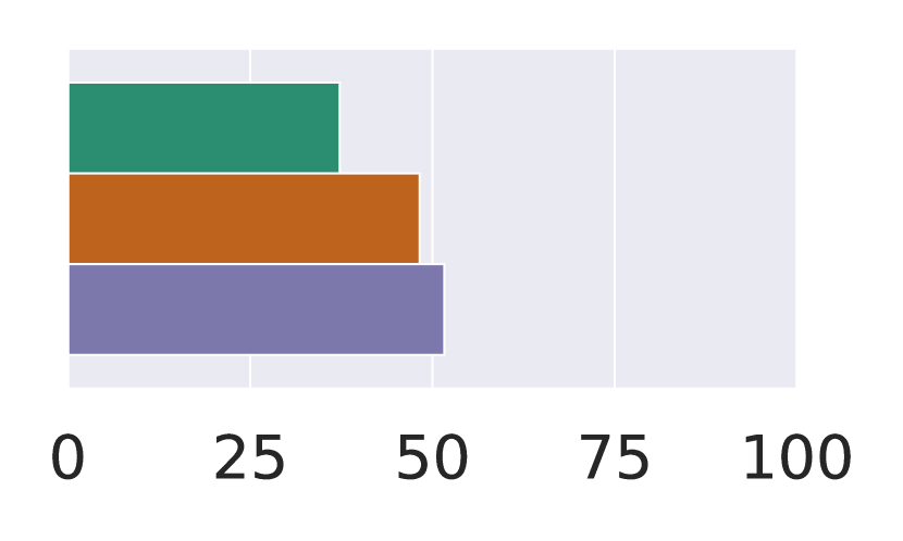
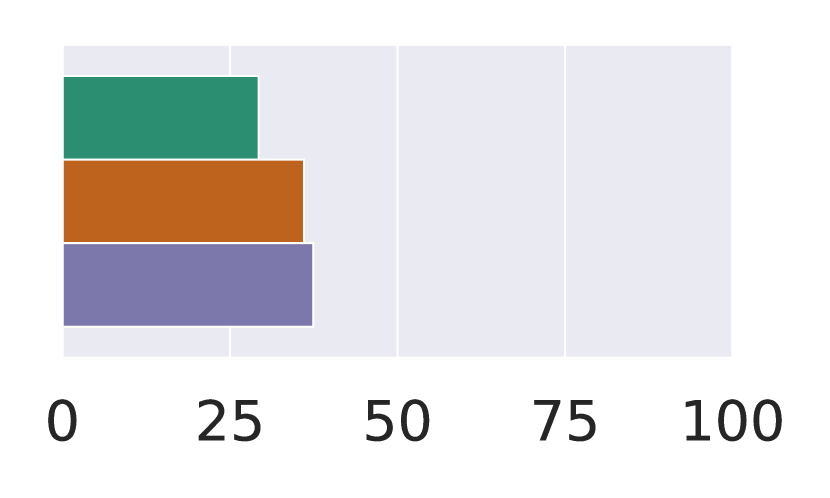
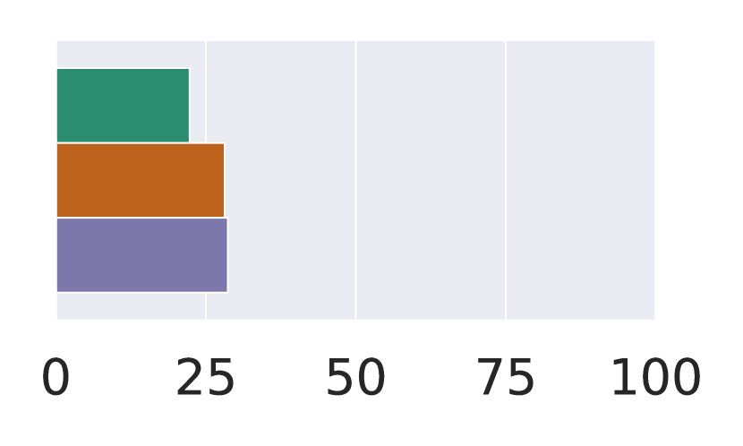
EM

Figure 7: Results of comment generation models with filtering near-duplicates using the $\mathtt{same\_code}$ configuration, on TestC sets.

Train	MP	CP	MP	T	CP	T
Test	$\text{MP}\cap\text{CP}$		$\text{MP}\cap\text{T}$		$\text{CP}\cap\text{T}$
$\blacktriangledown$ Precision [%]
Code2Vec	53.4	17.1	61.8	53.9	13.8	48.2
Code2Seq	50.4	38.7	49.8	46.4	34.5	42.9
$\blacktriangledown$ Recall [%]
Code2Vec	51.6	14.6	60.2	52.2	12.3	46.6
Code2Seq	41.2	28.7	41.7	37.7	25.9	34.9
$\blacktriangledown$ F1 [%]
Code2Vec	51.7	14.9	60.4	52.5	12.4	46.8
Code2Seq	44.0	31.6	44.0	40.1	28.2	37.0
$\blacktriangledown$ EM [%]
Code2Vec	35.0	5.0	47.4	43.4	α4.9	36.1
Code2Seq	14.6	6.4	16.7	14.1	α5.7	10.9

Table 10: Method naming models’ results with filtering near-duplicates using the $\mathtt{same\_code}$ configuration, on TestC sets.

Train	MP	CP	MP	T	CP	T
Test	$\text{MP}\cap\text{CP}$		$\text{MP}\cap\text{T}$		$\text{CP}\cap\text{T}$
Precision
Recall
F1
EM

Figure 8: Results of method naming models with filtering near-duplicates using the $\mathtt{same\_code}$ configuration, on TestC sets.

Train	MP	CP	MP	T	CP	T
Test	$\text{MP}\cap\text{CP}$		$\text{MP}\cap\text{T}$		$\text{CP}\cap\text{T}$
$\blacktriangledown$ BLEU [%]
DeepComHybrid	20.9	10.2	20.9	15.0	9.4	13.2
Seq2Seq	29.3	α12.6	27.5	18.6	β11.3	16.7
Transformer	32.9	α12.6	30.5	19.8	β11.6	17.8
$\blacktriangledown$ METEOR [%]
DeepComHybrid	31.4	17.1	δ30.6	23.6	16.4	21.4
Seq2Seq	41.4	γ20.2	38.6	29.1	ϵ19.6	27.1
Transformer	45.2	γ20.2	42.0	δ30.8	ϵ19.3	28.4
$\blacktriangledown$ ROUGE-L [%]
DeepComHybrid	37.3	23.3	ζ35.9	29.3	22.3	θ27.6
Seq2Seq	48.2	28.8	45.2	ζ36.0	ηθ28.1	34.5
Transformer	51.6	29.7	48.3	37.4	η28.7	36.0
$\blacktriangledown$ EM [%]
DeepComHybrid	1.7	ικ0.0	2.6	0.0	τπ0.1	στ0.4
Seq2Seq	6.4	ιλ0.3	μ7.0	ν0.7	τρσ0.1	υ1.0
Transformer	7.6	κλ0.3	μ7.4	ν1.1	πρτ0.2	υ1.2

Table 11: Comment generation models’ results with filtering near-duplicates using the $\mathtt{same\_summary}$ configuration, on TestC sets.

Train	MP	CP	MP	T	CP	T
Test	$\text{MP}\cap\text{CP}$		$\text{MP}\cap\text{T}$		$\text{CP}\cap\text{T}$
BLEU
METEOR
ROUGE-L
EM

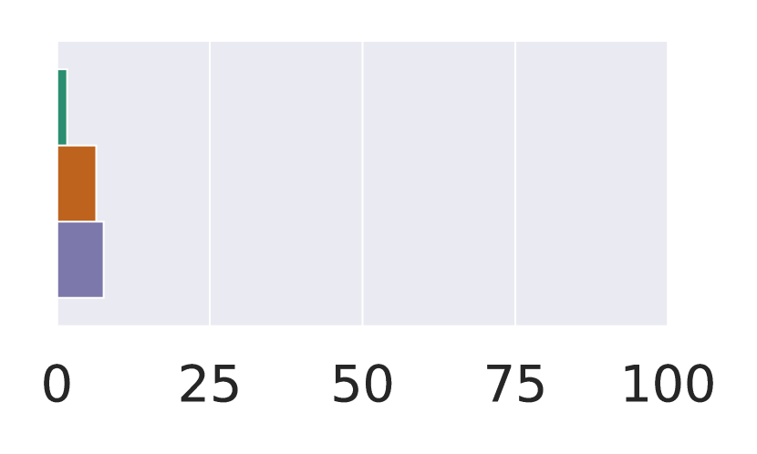
Figure 9: Results of comment generation models with filtering near-duplicates using the $\mathtt{same\_summary}$ configuration, on TestC sets.

  • comment generation: Table 11, Figure 9.

Train	MP	CP	MP	T	CP	T
Test	$\text{MP}\cap\text{CP}$		$\text{MP}\cap\text{T}$		$\text{CP}\cap\text{T}$
Precision
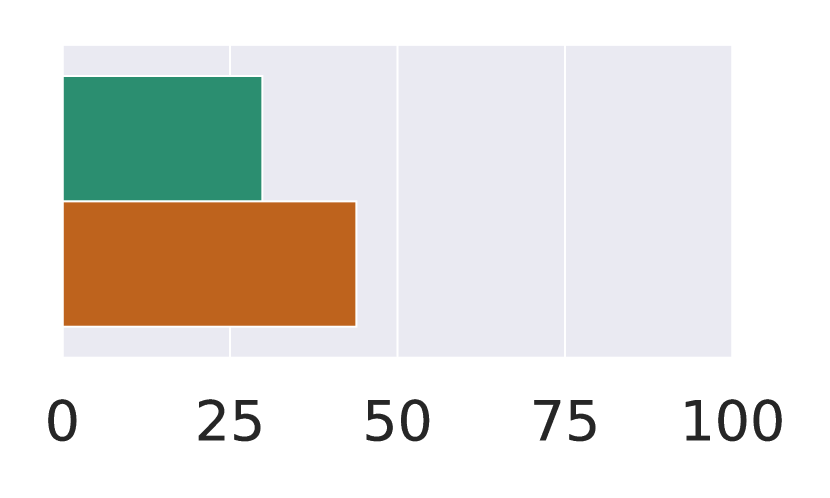
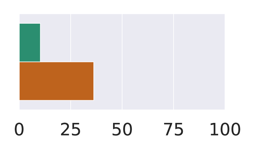
Recall
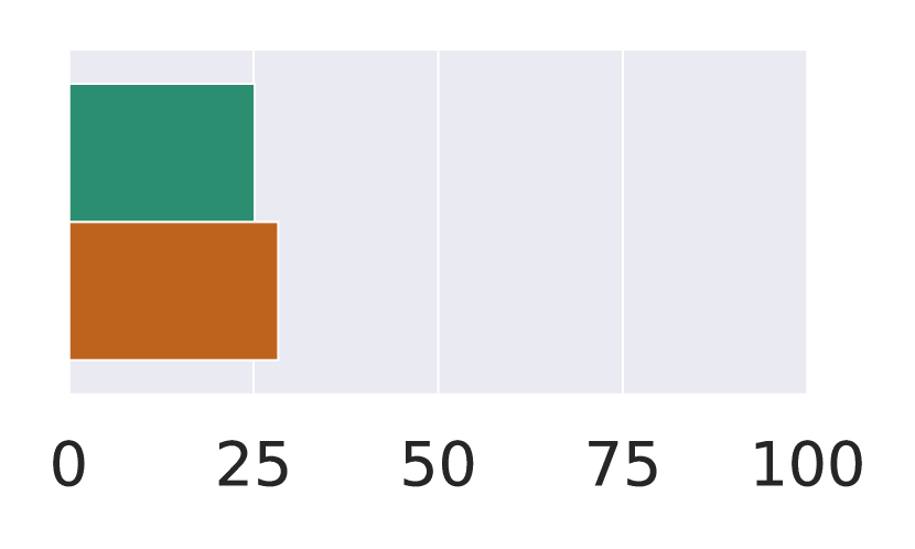
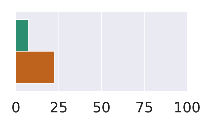
F1
EM

Figure 10: Results of method naming models with filtering near-duplicates using the $\mathtt{same\_summary}$ configuration, on TestC sets.

  • method naming: Table 12, Figure 10.

• Using $\mathtt{high\_similarity}$ configuration:

  • comment generation: Table 13, Figure 11.

  • method naming: Table 14, Figure 12.

We can draw several conclusions. First of all, our findings in Section 5.4 still hold. The metrics of $\mathtt{same\_code}$ are closest to the metrics of not filtering near-duplicates, which indicates that this filtering configuration has little impact on evaluation results. On the contrary, the metrics of $\mathtt{same\_summary}$ and $\mathtt{high\_similarity}$ are lower than the metrics of not filtering near-duplicates, which means the models become less effective. This indicates that current ML models for code summarization are better at following the samples in the training set than generating novel summaries.

Appendix C Data Collection Details

		MP				CP				T				$\text{MP}\cap\text{CP}$	$\text{MP}\cap\text{T}$	$\text{CP}\cap\text{T}$
Statistic		Train	Val	TestS		Train	Val	TestS		Train	Val	TestS		TestC
#Sample		50,879	7,569	14,956		50,879	8,938	15,661		50,879	11,312	9,870		3,362	2,013	2,220
	avg	89.84	92.97	93.02		86.23	93.12	106.11		85.83	104.88	105.36		106.83	106.15	125.01
	$\leq$100[%]	74.97	73.62	74.28		76.36	73.42	69.82		76.55	70.66	68.38		70.32	68.16	59.82
	$\leq$150[%]	84.47	83.71	83.96		85.59	83.42	80.38		85.70	81.24	79.75		80.07	79.78	73.69
len(code)	$\leq$200[%]	89.86	89.42	89.30		90.67	89.24	86.69		90.74	87.05	86.80		85.81	86.74	82.52
	avg	11.98	12.07	12.03		11.96	12.09	12.13		12.00	12.20	12.04		12.16	12.10	12.20
	$\leq$20[%]	88.91	88.73	89.05		88.74	88.70	89.53		88.83	88.56	88.99		90.10	88.72	88.29
	$\leq$30[%]	97.12	97.21	97.33		97.12	96.65	97.54		97.29	96.96	96.53		97.95	96.77	96.80
len(com)	$\leq$50[%]	99.61	99.67	99.64		99.61	99.62	99.69		99.68	99.62	99.37		99.58	99.45	99.37

Table 7: Comment generation dataset metrics.

		MP				CP				T				$\text{MP}\cap\text{CP}$	$\text{MP}\cap\text{T}$	$\text{CP}\cap\text{T}$
Statistic		Train	Val	TestS		Train	Val	TestS		Train	Val	TestS		TestC
#Sample		50,879	7,523	14,796		50,879	8,811	15,332		50,879	11,223	9,807		3,344	2,011	2,211
	avg	88.15	91.70	91.97		84.56	92.28	105.87		84.17	103.71	104.09		105.42	104.38	123.46
	$\leq$100[%]	75.45	74.00	74.64		76.81	73.57	69.91		77.04	71.00	68.79		70.93	68.72	60.33
	$\leq$150[%]	84.75	83.89	84.08		85.83	83.52	80.37		85.96	81.44	79.95		80.17	80.01	74.04
len(code)	$\leq$200[%]	90.03	89.47	89.36		90.80	89.32	86.63		90.87	87.16	86.96		85.94	86.92	82.81
	avg	2.52	2.52	2.56		2.50	2.31	2.71		2.50	2.63	2.64		2.70	2.70	2.82
	$\leq$2[%]	57.27	56.40	55.52		57.82	64.60	50.39		57.45	55.67	53.99		49.55	50.92	46.54
	$\leq$3[%]	81.31	81.72	80.64		81.64	84.67	78.10		82.12	78.29	78.48		78.20	77.13	73.77
len(name)	$\leq$6[%]	98.54	98.67	98.53		98.47	98.91	98.62		98.84	97.61	98.00		98.92	98.01	98.24

Table 8: Method naming dataset metrics.

This section extends §5.2 and describes our data collection process in details. Overall, our datasets are collected and processed following the steps in §4 and Appendix A. We started by collecting samples of methods with comments from open-source GitHub projects, and then performed task-specific processing to get the dataset for each task.

Selecting projects. We initially chose 1,793 popular Java projects on GitHub: 1,000 Java projects with the highest number of stars (indicating how many GitHub users bookmarked a project) and another 793 Java projects whose owner is one of the famous open-source organizations on GitHub. We chose to use only Java projects because most prior work focused on this language (see Table 1). Then, we only kept the projects meeting the following criteria: (1) the number of stars should be larger than 20; (2) the lines of code of the project (as reported by GitHub API) should be in the range of $[10^{6},2\times 10^{6}]$, to keep the number of samples balanced across projects; (3) the project should have at least one commit after $\text{Jan }1^{st}$ 2018. 160 projects satisfied all the criteria.

Collecting the raw dataset. We set the timestamps $\tau^{-2}$ to 2019 $\text{Jan }1^{st}$, $\tau^{-1}$ to 2020 $\text{Jan }1^{st}$, and $\tau$ to 2021 $\text{Jan }1^{st}$. For each project and for each year in [2019, 2020, 2021], we identified the last commit in the project before $\text{Jan }1^{st}$ of that year, checked-out to that commit, used JavaParser to parse all Java files, and collected samples of Java methods in the form of (code, comment, name, project, year) tuples, where the comment is the first sentence in the JavaDoc of the method. We discarded the samples where: (1) the code or the comment contains non-English characters (157 and 5,139 cases respectively); (2) the code is longer than 10,000 characters (60 cases); (3) the method body is empty, i.e., abstract method (77,769 cases); (4) the comment is empty after removing tags such as $\mathtt{@inheritDoc}$ (21,779 cases). If two samples are identical except for the “year” label, we would keep the one with the earliest year (e.g., two samples from 2018 and 2019 years have identical code, comment, name, and project, so we only keep the 2018 one). We ended up with 77,475 samples in the raw dataset.

Then, we follow the steps described in §4 to split the raw dataset into Train, Val, TestS sets for each methodology and TestC set for each pair of methodologies. The splitting ratios (for in-project and cross-project splits) are: $r_{x}=70\%,r_{y}=10\%,r_{z}=20\%$.

Comment generation. Table 7 shows the statistics of the comment generation dataset. The rows, from top to bottom, are: the number of samples; the average number of subtokens in code; the percentage of samples whose number of subtokens in the code is less than 100, 150, 200; the average number of subtokens in comments; the percentage of samples whose number of subtokens in the comment is less than 20, 30, 50. Figure 5 visualizes the distributions of the number of subtokens in code (x-axis) and the number of subtokens in comments (y-axis).

Method naming. For each sample, we replaced the appearances of its name from its code to the special token “METHODNAMEMASK” such that the models cannot cheat by looking for the name in the signature line or in the method body of recursive methods. Table 8 shows the statistics of the method naming dataset. The rows, from top to bottom, are: the number of samples; the average number of subtokens in code; the percentage of samples whose number of subtokens in the code is less than 100, 150, 200; the average number of subtokens in names; the percentage of samples whose number of subtokens in the name is less than 2, 3, 6. Figure 6 visualizes the distributions of the number of subtokens in code (x-axis) and the number of subtokens in names (y-axis).

	ATrain	Val	TestS		TestC
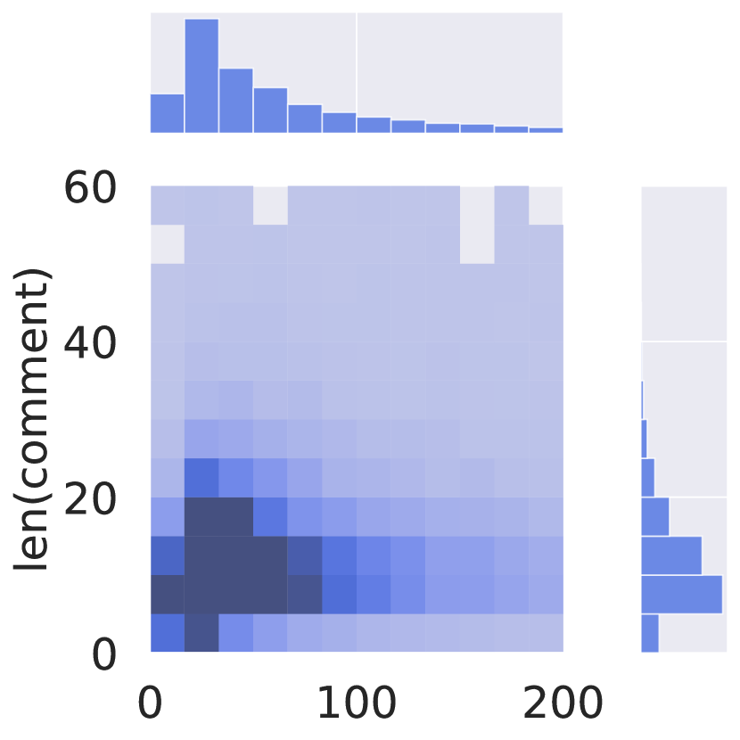
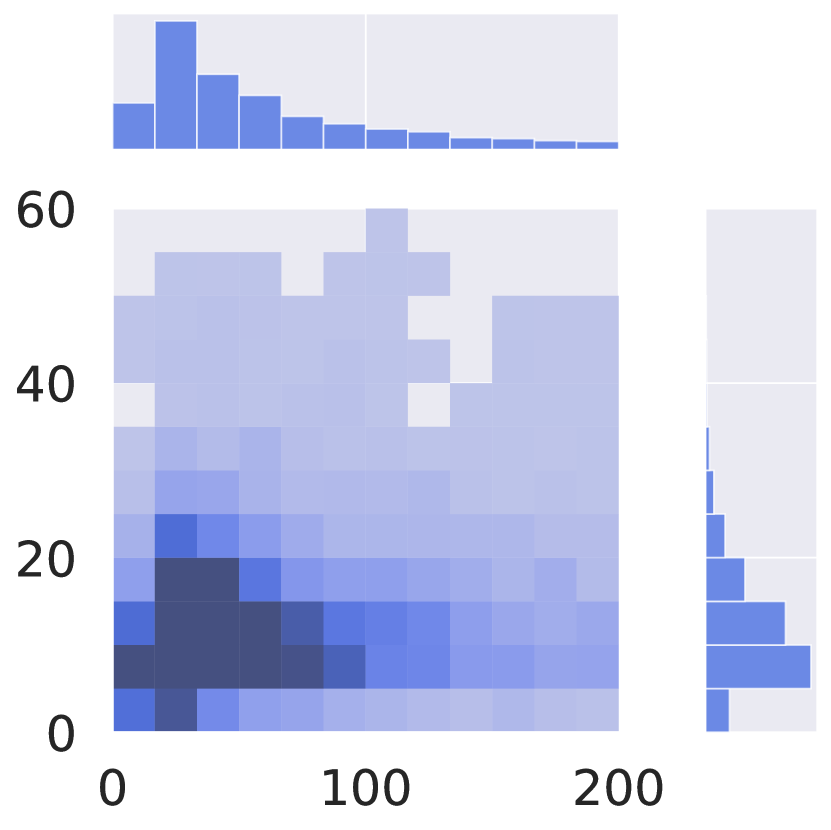
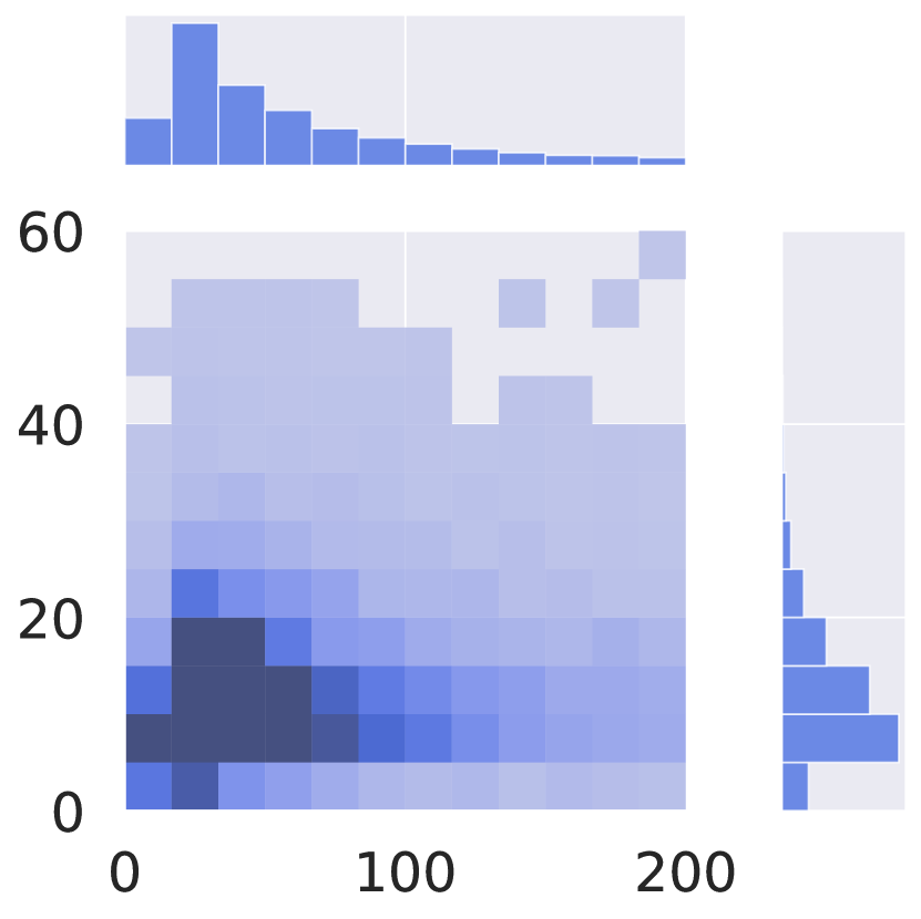
MP				$\text{MP}\cap\text{CP}$
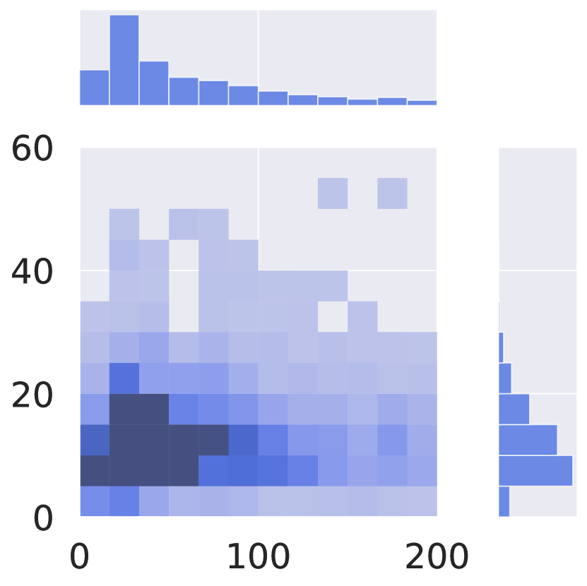
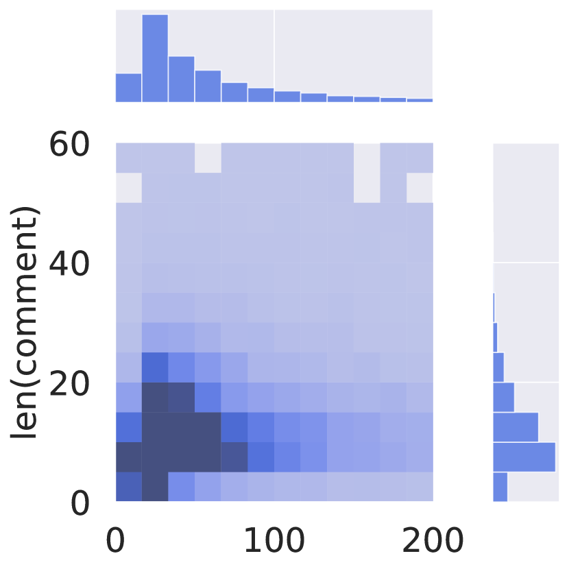
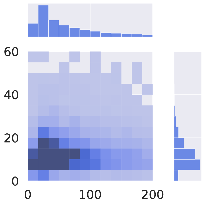
CP				$\text{MP}\cap\text{T}$
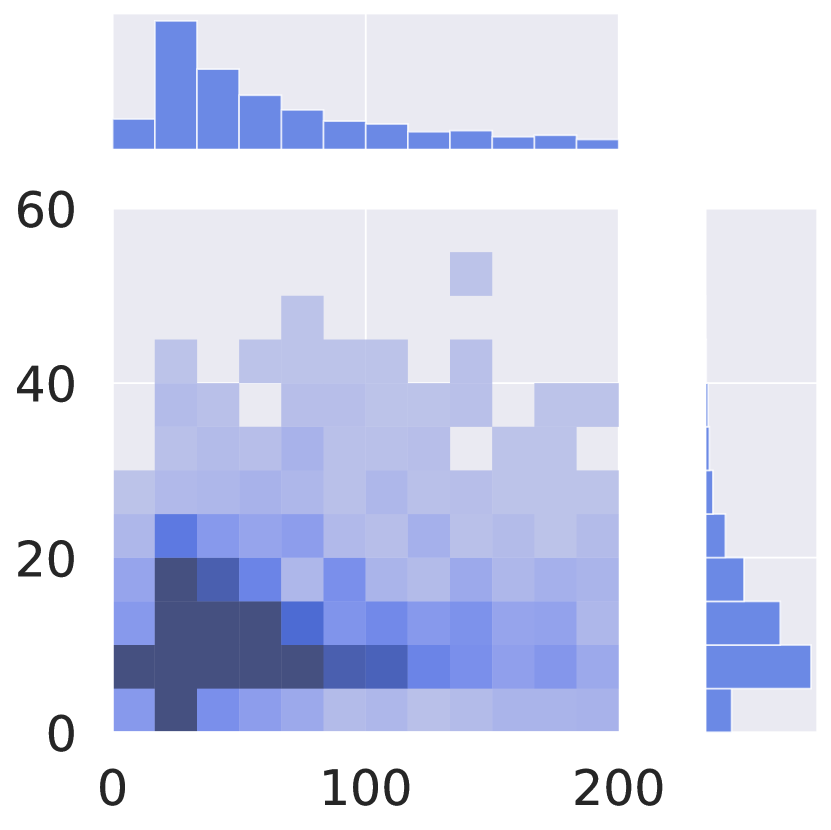
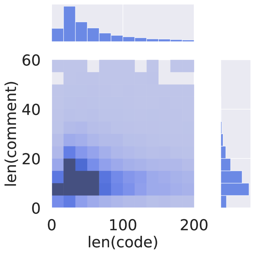
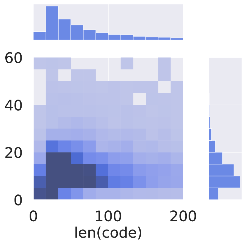
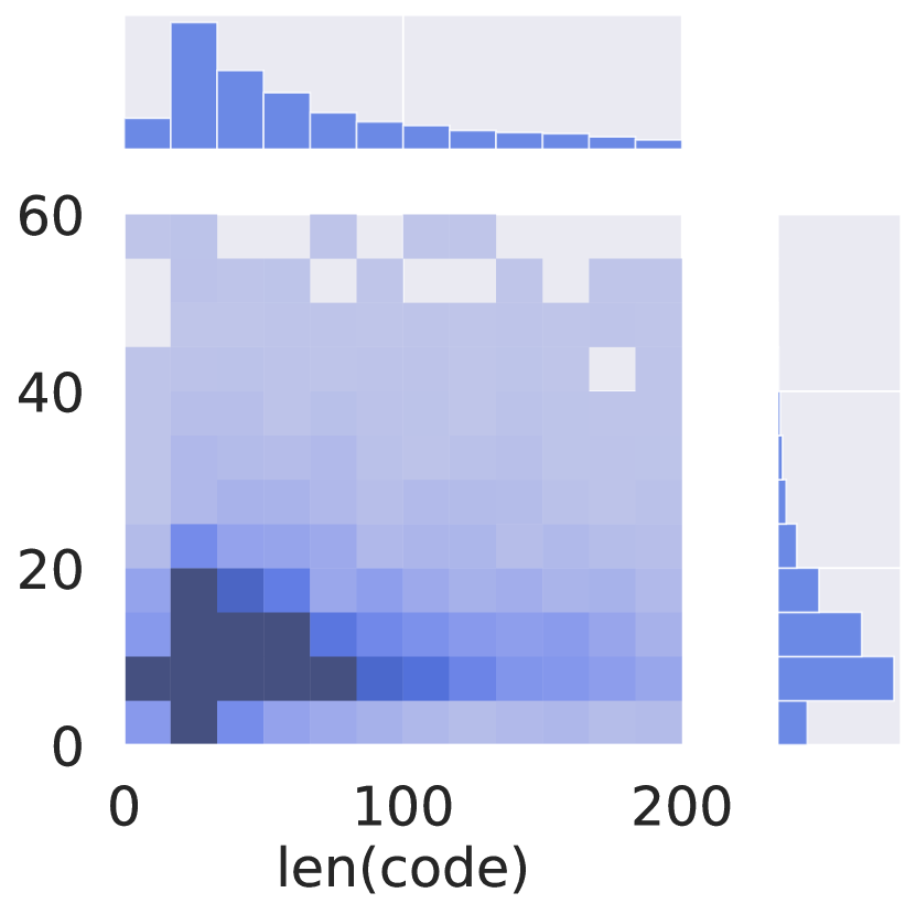
T				$\text{CP}\cap\text{T}$

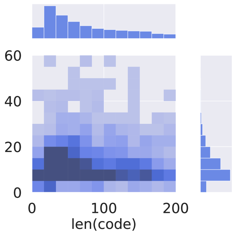
Figure 5: Distributions of the number of subtokens in code (x-axis) and the number of subtokens in comments (y-axis) in our comment generation dataset.

	ATrain	Val	TestS		TestC
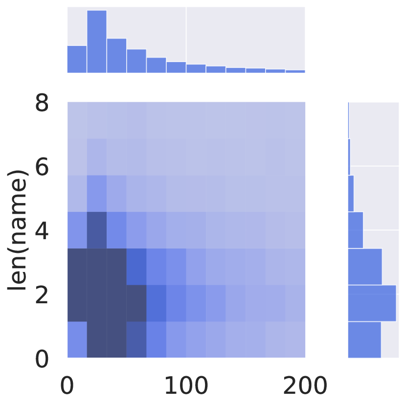
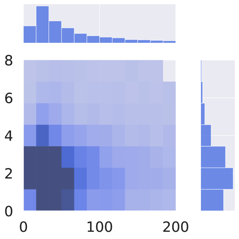
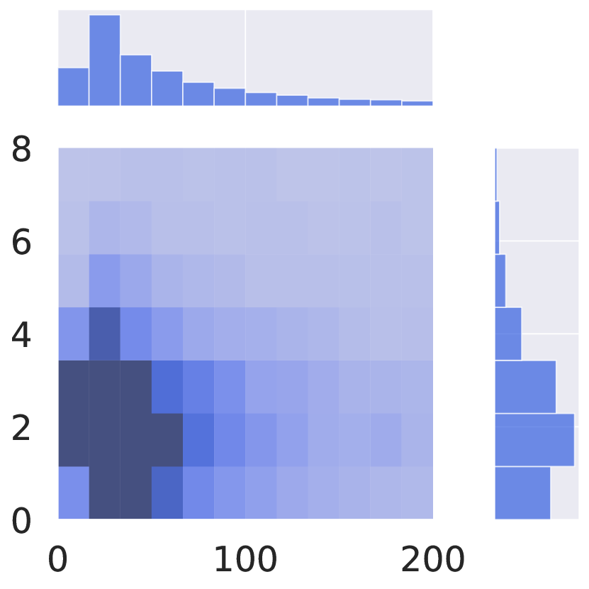
MP				$\text{MP}\cap\text{CP}$
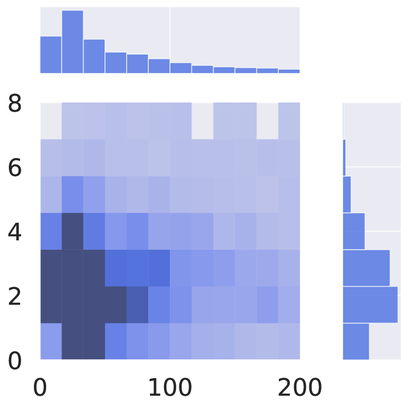
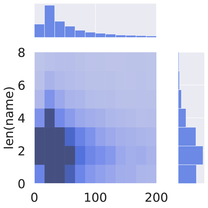
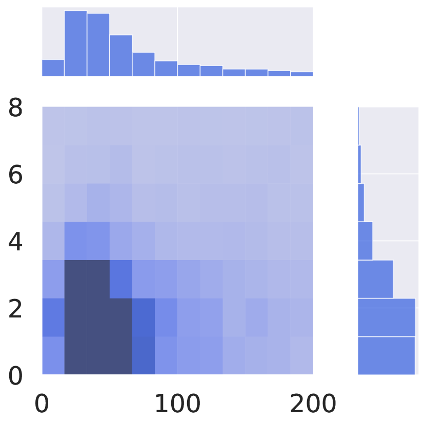
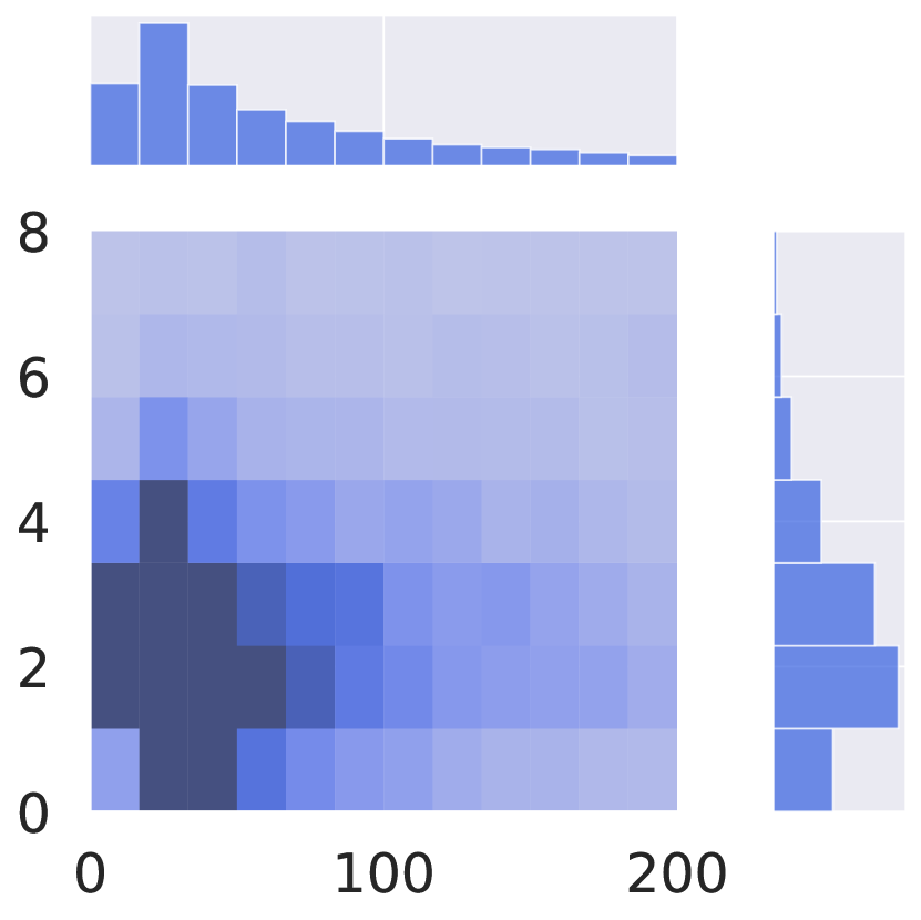
CP				$\text{MP}\cap\text{T}$
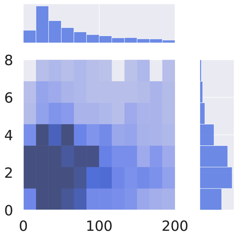
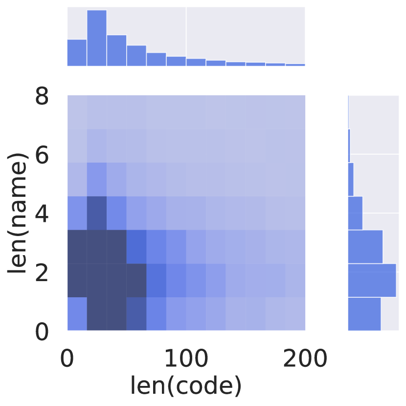
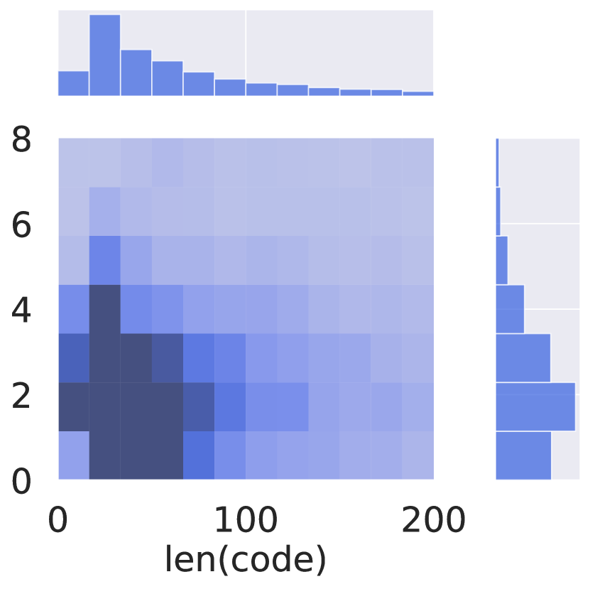
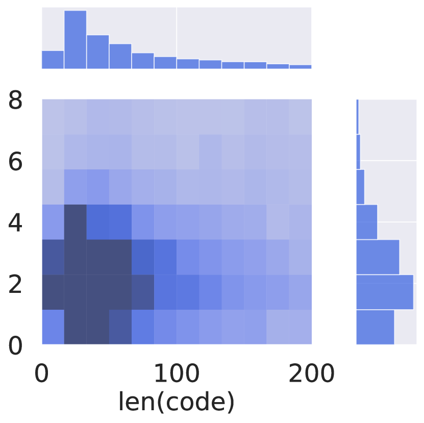
T				$\text{CP}\cap\text{T}$

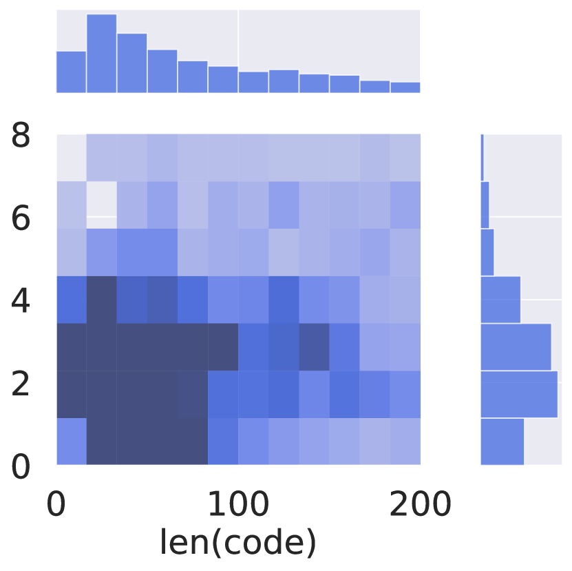
Figure 6: Distributions of the number of subtokens in code (x-axis) and the number of subtokens in names (y-axis) in our method naming dataset.

Appendix D Experiments Details

This section presents details of our experiments to support their reproducibility.

Computing infrastructure. We run our experiments on a machine with four NVIDIA 1080-TI GPUs and two Intel Xeon E5-2620 v4 CPUs.

Estimated runtime of models. The approximate model training time are: DeepComHybrid 7 days; Seq2Seq 4 hours; Transformer 10 hours; Code2Seq 4 hours; Code2Vec 15 minutes. The evaluation time is around 1–10 minutes per model per evaluation set.

Number of parameters. The number of parameters in each model are: DeepComHybrid 15.6M; Seq2Seq 31.3M; Transformer 68.2M; Code2Seq 5.7M; Code2Vec 33.1M.

Random seeds. The random seed used for preparing the dataset (performing in-project and cross-project splits) is: 7. The random seeds used for the three times of training are: 4182, 99243, 3705.

Reproducibility of prior work. We used the replication packages provided in the original papers of the models when possible. We made (small) updates to all models to: (1) upgrade outdated data processing code (because of our dataset contains samples with new programming language features that were not considered in the past); (2) export evaluation results in the format compatible with our scripts. We integrated these updates in our replication package.

Appendix E Additional Experiment Results

We present the following additional tables and figures to help characterize our experiments results and support our findings:

• Evaluation results on the Val and TestS sets.

  • comment generation: Table 15.

  • method naming: Table 16.

• Bar plots of the automatic metrics per sample.

  • comment generation:

    • on the TestC sets: Figure 13.

    • on the Val and TestS sets: Figure 14.

  • method naming:

    • on the TestC sets: Figure 15.

    • on the Val and TestS sets: Figure 16.

Train	MP	CP	MP	T	CP	T
Test	$\text{MP}\cap\text{CP}$		$\text{MP}\cap\text{T}$		$\text{CP}\cap\text{T}$
$\blacktriangledown$ BLEU [%]
DeepComHybrid	37.8	10.4	β48.8	38.5	10.5	36.8
Seq2Seq	48.7	α12.6	59.2	β50.3	12.5	46.4
Transformer	52.8	α12.9	63.2	53.5	13.3	49.1
$\blacktriangledown$ METEOR [%]
DeepComHybrid	46.4	17.1	δ55.6	45.5	17.2	44.0
Seq2Seq	57.4	γ19.9	65.5	δ56.9	ϵ20.1	53.3
Transformer	61.5	γ20.0	69.3	59.9	ϵ20.3	55.8
$\blacktriangledown$ ROUGE-L [%]
DeepComHybrid	51.0	22.8	59.3	49.6	22.5	48.5
Seq2Seq	62.6	28.2	69.7	61.4	28.0	58.6
Transformer	66.1	29.0	72.8	63.9	29.0	60.8
$\blacktriangledown$ EM [%]
DeepComHybrid	22.4	ζη0.5	36.1	26.8	ικ1.0	26.0
Seq2Seq	31.5	ζθ0.6	46.6	38.9	ιλ0.8	35.4
Transformer	34.7	ηθ0.8	50.4	41.9	κλ1.2	38.2

Table 9: Comment generation models’ results with filtering near-duplicates using the $\mathtt{same\_code}$ configuration, on TestC sets.

Train	MP	CP	MP	T	CP	T
Test	$\text{MP}\cap\text{CP}$		$\text{MP}\cap\text{T}$		$\text{CP}\cap\text{T}$
$\blacktriangledown$ Precision [%]
Code2Vec	31.7	16.8	29.8	17.3	10.3	16.4
Code2Seq	50.1	42.4	43.9	40.5	36.2	39.1
$\blacktriangledown$ Recall [%]
Code2Vec	α26.8	11.5	β25.2	13.0	7.2	12.1
Code2Seq	34.7	α27.1	28.3	β25.5	22.4	24.9
$\blacktriangledown$ F1 [%]
Code2Vec	28.1	12.9	26.5	14.3	8.0	13.3
Code2Seq	39.9	31.9	33.3	30.3	26.5	29.4
$\blacktriangledown$ EM [%]
Code2Vec	γ0.1	γ0.0	0.5	0.1	δ0.0	δ0.1
Code2Seq	2.7	0.9	0.9	1.4	0.8	2.1

Table 12: Method naming models’ results with filtering near-duplicates using the $\mathtt{same\_summary}$ configuration, on TestC sets.

Train	MP	CP	MP	T	CP	T
Test	$\text{MP}\cap\text{CP}$		$\text{MP}\cap\text{T}$		$\text{CP}\cap\text{T}$
$\blacktriangledown$ BLEU [%]
DeepComHybrid	16.3	10.3	β13.5	10.7	9.5	δϵ11.2
Seq2Seq	24.4	α13.0	19.2	β13.8	γδ11.6	14.4
Transformer	26.8	α13.1	21.4	14.6	γϵ11.6	15.1
$\blacktriangledown$ METEOR [%]
DeepComHybrid	26.1	17.3	22.1	18.2	16.4	η19.1
Seq2Seq	36.1	ζ20.8	29.9	23.3	20.1	24.4
Transformer	39.1	ζ20.8	32.5	24.5	η19.3	25.4
$\blacktriangledown$ ROUGE-L [%]
DeepComHybrid	32.2	23.2	27.6	23.6	22.4	25.4
Seq2Seq	43.4	29.1	37.0	30.3	θ28.8	32.2
Transformer	46.0	29.9	39.6	31.6	θ28.7	33.3
$\blacktriangledown$ EM [%]
DeepComHybrid	0.9	ι0.0	0.9	ντ0.0	ρσ0.1	υϕ0.4
Seq2Seq	λ4.4	ικ0.3	μ2.2	νπ0.1	ρτυ0.2	χ0.9
Transformer	λ5.3	κ0.3	μ2.2	τπ0.1	στϕ0.2	χ1.2

Table 13: Comment generation models’ results with filtering near-duplicates using the $\mathtt{high\_similarity}$ configuration, on TestC sets.

Train	MP	CP	MP	T	CP	T
Test	$\text{MP}\cap\text{CP}$		$\text{MP}\cap\text{T}$		$\text{CP}\cap\text{T}$
BLEU
METEOR
ROUGE-L
EM

Figure 11: Results of comment generation models with filtering near-duplicates using the $\mathtt{high\_similarity}$ configuration, on TestC sets.

Train	MP	CP	MP	T	CP	T
Test	$\text{MP}\cap\text{CP}$		$\text{MP}\cap\text{T}$		$\text{CP}\cap\text{T}$
$\blacktriangledown$ Precision [%]
Code2Vec	26.5	15.2	26.2	15.2	10.3	14.8
Code2Seq	47.0	40.3	41.3	39.4	35.7	38.0
$\blacktriangledown$ Recall [%]
Code2Vec	22.1	10.5	21.7	11.3	7.1	10.9
Code2Seq	32.2	25.9	26.7	24.7	21.9	24.2
$\blacktriangledown$ F1 [%]
Code2Vec	23.3	11.7	23.0	12.5	8.0	12.0
Code2Seq	37.1	30.4	31.3	29.3	26.1	28.5
$\blacktriangledown$ EM [%]
Code2Vec	α0.1	α0.0	0.6	0.1	β0.0	β0.1
Code2Seq	2.5	1.0	1.0	1.7	0.9	2.3

Table 14: Method naming models’ results with filtering near-duplicates using the $\mathtt{high\_similarity}$ configuration, on TestC sets.

Train	MP	CP	MP	T	CP	T
Test	$\text{MP}\cap\text{CP}$		$\text{MP}\cap\text{T}$		$\text{CP}\cap\text{T}$
Precision
Recall
F1
EM

Figure 12: Results of method naming models with filtering near-duplicates using the $\mathtt{high\_similarity}$ configuration, on TestC sets.

Train	MP		CP		T
Test	Val	TestS	Val	TestS	Val	TestS
$\blacktriangledown$ BLEU [%]
DeepComHybrid	48.9	49.6	11.8	11.6	48.3	43.1
Seq2Seq	57.7	58.6	α13.7	β13.7	58.4	53.0
Transformer	61.5	62.5	α14.2	β14.2	62.2	56.4
$\blacktriangledown$ METEOR [%]
DeepComHybrid	56.6	57.2	17.9	18.4	55.0	50.1
Seq2Seq	65.1	66.0	γ19.9	δ21.2	64.8	59.4
Transformer	68.9	69.8	γ19.5	δ21.1	68.2	62.7
$\blacktriangledown$ ROUGE-L [%]
DeepComHybrid	60.3	60.9	22.4	24.1	58.3	53.9
Seq2Seq	69.5	70.0	ϵ27.3	ζ29.6	68.5	63.9
Transformer	72.7	73.3	ϵ27.4	ζ30.2	71.3	66.7
$\blacktriangledown$ EM [%]
DeepComHybrid	34.3	35.2	η3.4	θι1.6	36.5	31.0
Seq2Seq	42.3	43.5	2.2	θκ1.3	45.8	40.8
Transformer	45.7	46.9	η3.3	ικ1.8	50.5	44.4

Table 15: Comment generation models’ results on Val and TestS sets.

Train	MP	CP	MP	T	CP	T
Test	$\text{MP}\cap\text{CP}$		$\text{MP}\cap\text{T}$		$\text{CP}\cap\text{T}$
BLEU
METEOR
ROUGE-L
EM

Figure 13: Results of comment generation models on common test sets.

Train	MP		CP		T
Test	Val	TestS	Val	TestS	Val	TestS
BLEU
METEOR
ROUGE-L
EM

Figure 14: Results of comment generation models on validation and standard test sets.

Train	MP		CP		T
Test	Val	TestS	Val	TestS	Val	TestS
$\blacktriangledown$ Precision [%]
Code2Vec	61.9	62.3	14.6	18.6	63.1	57.7
Code2Seq	53.2	53.1	27.7	39.3	47.8	47.9
$\blacktriangledown$ Recall [%]
Code2Vec	60.4	60.7	13.7	16.3	61.3	56.0
Code2Seq	44.9	44.9	22.4	30.1	39.5	39.8
$\blacktriangledown$ F1 [%]
Code2Vec	60.5	60.9	13.7	16.6	61.6	56.3
Code2Seq	47.2	47.2	23.6	32.7	41.8	42.0
$\blacktriangledown$ EM [%]
Code2Vec	46.9	47.1	α8.9	β6.6	53.4	47.3
Code2Seq	20.2	19.7	α9.1	β8.0	17.0	15.8

Table 16: Method naming models’ results on Val and TestS sets.

Train	MP	CP	MP	T	CP	T
Test	$\text{MP}\cap\text{CP}$		$\text{MP}\cap\text{T}$		$\text{CP}\cap\text{T}$
Precision
Recall
F1
EM

Figure 15: Results of method naming models on common test sets.

Train	MP		CP		T
Test	Val	TestS	Val	TestS	Val	TestS
Precision
Recall
F1
EM

Figure 16: Results of method naming models on validation and standard test sets.

References

- Ahmad et al. (2020) Wasi Ahmad, Saikat Chakraborty, Baishakhi Ray, and Kai-Wei Chang. 2020. A transformer-based approach for source code summarization. In Annual Meeting of the Association for Computational Linguistics, pages 4998–5007.
- Ahmad et al. (2021) Wasi Ahmad, Saikat Chakraborty, Baishakhi Ray, and Kai-Wei Chang. 2021. Unified pre-training for program understanding and generation. In Conference of the North American Chapter of the Association for Computational Linguistics: Human Language Technologies, pages 2655–2668.
- Allamanis (2019) Miltiadis Allamanis. 2019. The adverse effects of code duplication in machine learning models of code. In International Symposium on New Ideas, New Paradigms, and Reflections on Programming and Software, pages 143–153.
- Allamanis et al. (2015) Miltiadis Allamanis, Earl T. Barr, Christian Bird, and Charles Sutton. 2015. Suggesting accurate method and class names. In Joint European Software Engineering Conference and Symposium on the Foundations of Software Engineering, pages 38–49.
- Allamanis et al. (2016) Miltiadis Allamanis, Hao Peng, and Charles Sutton. 2016. A convolutional attention network for extreme summarization of source code. In International Conference on Machine Learning, pages 2091–2100.
- Alon et al. (2019a) Uri Alon, Shaked Brody, Omer Levy, and Eran Yahav. 2019a. code2seq: Generating sequences from structured representations of code. In International Conference on Learning Representations.
- Alon et al. (2019b) Uri Alon, Meital Zilberstein, Omer Levy, and Eran Yahav. 2019b. code2vec: Learning distributed representations of code. Proceedings of the ACM on Programming Languages, 3(POPL):1–29.
- Banerjee and Lavie (2005) Satanjeev Banerjee and Alon Lavie. 2005. METEOR: An automatic metric for MT evaluation with improved correlation with human judgments. In Workshop on Intrinsic and Extrinsic Evaluation Measures for Machine Translation and/or Summarization, pages 65–72.
- Bender et al. (2021) Emily M. Bender, Timnit Gebru, Angelina McMillan-Major, and Shmargaret Shmitchell. 2021. On the dangers of stochastic parrots: Can language models be too big? In Conference on Fairness, Accountability, and Transparency, pages 610–623.
- Berg-Kirkpatrick et al. (2012) Taylor Berg-Kirkpatrick, David Burkett, and Dan Klein. 2012. An empirical investigation of statistical significance in NLP. In Joint Conference on Empirical Methods in Natural Language Processing and Computational Natural Language Learning, pages 995–1005.
- Cai et al. (2020) Ruichu Cai, Zhihao Liang, Boyan Xu, Zijian Li, Yuexing Hao, and Yao Chen. 2020. TAG : Type auxiliary guiding for code comment generation. In Annual Meeting of the Association for Computational Linguistics, pages 291–301.
- Chen et al. (2021) Mark Chen, Jerry Tworek, Heewoo Jun, Qiming Yuan, Henrique Ponde de Oliveira Pinto, Jared Kaplan, Harri Edwards, Yuri Burda, Nicholas Joseph, Greg Brockman, et al. 2021. Evaluating large language models trained on code. arXiv preprint arXiv:2107.03374.
- D’Ambros et al. (2012) Marco D’Ambros, Michele Lanza, and Romain Robbes. 2012. Evaluating defect prediction approaches: A benchmark and an extensive comparison. Empirical Software Engineering, 17(4-5):531–577.
- Feng et al. (2020) Zhangyin Feng, Daya Guo, Duyu Tang, Nan Duan, Xiaocheng Feng, Ming Gong, Linjun Shou, Bing Qin, Ting Liu, Daxin Jiang, and Ming Zhou. 2020. CodeBERT: A pre-trained model for programming and natural languages. In Findings of the Association for Computational Linguistics: EMNLP, pages 1536–1547.
- Fernandes et al. (2019) Patrick Fernandes, Miltiadis Allamanis, and Marc Brockschmidt. 2019. Structured neural summarization. In International Conference on Learning Representations.
- Fluri et al. (2007) Beat Fluri, Michael Würsch, and Harald C. Gall. 2007. Do code and comments co-evolve? on the relation between source code and comment changes. In Working Conference on Reverse Engineering, pages 70–79.
- Gros et al. (2020) David Gros, Hariharan Sezhiyan, Prem Devanbu, and Zhou Yu. 2020. Code to comment “translation”: data, metrics, baselining & evaluation. In Automated Software Engineering, pages 746–757.
- Guo et al. (2021) Daya Guo, Shuo Ren, Shuai Lu, Zhangyin Feng, Duyu Tang, Shujie Liu, Long Zhou, Nan Duan, Alexey Svyatkovskiy, Shengyu Fu, Michele Tufano, Shao Kun Deng, Colin Clement, Dawn Drain, Neel Sundaresan, Jian Yin, Daxin Jiang, and Ming Zhou. 2021. GraphCodeBERT: Pre-training code representations with data flow. In International Conference on Learning Representations.
- Høst and Østvold (2009) Einar W. Høst and Bjarte M. Østvold. 2009. Debugging method names. In European Conference on Object-Oriented Programming, pages 294–317.
- Hu et al. (2018a) Xing Hu, Ge Li, Xin Xia, David Lo, and Zhi Jin. 2018a. Deep code comment generation. In International Conference on Program Comprehension, pages 200–210.
- Hu et al. (2020) Xing Hu, Ge Li, Xin Xia, David Lo, and Zhi Jin. 2020. Deep code comment generation with hybrid lexical and syntactical information. Empirical Software Engineering, 25(3):2179–2217.
- Hu et al. (2018b) Xing Hu, Ge Li, Xin Xia, David Lo, Shuai Lu, and Zhi Jin. 2018b. Summarizing source code with transferred API knowledge. In International Joint Conference on Artificial Intelligence, pages 2269–2275.
- Iyer et al. (2016) Srinivasan Iyer, Ioannis Konstas, Alvin Cheung, and Luke Zettlemoyer. 2016. Summarizing source code using a neural attention model. In Annual Meeting of the Association for Computational Linguistics, pages 2073–2083.
- Kamei et al. (2016) Yasutaka Kamei, Takafumi Fukushima, Shane McIntosh, Kazuhiro Yamashita, Naoyasu Ubayashi, and Ahmed E. Hassan. 2016. Studying just-in-time defect prediction using cross-project models. Empirical Software Engineering, 21(5).
- Lawrie et al. (2006) Dawn Lawrie, Christopher Morrell, Henry Feild, and David Binkley. 2006. What’s in a name? a study of identifiers. In International Conference on Program Comprehension, pages 3–12.
- LeClair et al. (2020) Alexander LeClair, Sakib Haque, Lingfei Wu, and Collin McMillan. 2020. Improved code summarization via a graph neural network. In International Conference on Program Comprehension, page 184–195.
- LeClair et al. (2019) Alexander LeClair, Siyuan Jiang, and Collin McMillan. 2019. A neural model for generating natural language summaries of program subroutines. In International Conference on Software Engineering, pages 795–806.
- LeClair and McMillan (2019) Alexander LeClair and Collin McMillan. 2019. Recommendations for datasets for source code summarization. In Conference of the North American Chapter of the Association for Computational Linguistics: Human Language Technologies, pages 3931–3937.
- Liang and Zhu (2018) Yuding Liang and Kenny Qili Zhu. 2018. Automatic generation of text descriptive comments for code blocks. In AAAI Conference on Artificial Intelligence, pages 5229–5236.
- Lin et al. (2021) Bo Lin, Shangwen Wang, Kui Liu, Xiaoguang Mao, and Tegawendé F Bissyandé. 2021. Automated comment update: How far are we? In International Conference on Program Comprehension, pages 36–46.
- Lin and Och (2004a) Chin-Yew Lin and Franz Josef Och. 2004a. Automatic evaluation of machine translation quality using longest common subsequence and skip-bigram statistics. In Annual Meeting of the Association for Computational Linguistics, pages 605–612.
- Lin and Och (2004b) Chin-Yew Lin and Franz Josef Och. 2004b. ORANGE: A method for evaluating automatic evaluation metrics for machine translation. In International Conference on Computational Linguistics, pages 501–507.
- Liu et al. (2020) Zhongxin Liu, Xin Xia, Meng Yan, and Shanping Li. 2020. Automating just-in-time comment updating. In Automated Software Engineering, pages 585–597.
- Lutellier et al. (2020) Thibaud Lutellier, Hung Viet Pham, Lawrence Pang, Yitong Li, Moshi Wei, and Lin Tan. 2020. CoCoNuT: Combining context-aware neural translation models using ensemble for program repair. In International Symposium on Software Testing and Analysis, pages 101–114.
- Nguyen et al. (2020) Son Nguyen, Hung Phan, Trinh Le, and Tien N. Nguyen. 2020. Suggesting natural method names to check name consistencies. In International Conference on Software Engineering, page 1372–1384.
- Nie et al. (2018) Pengyu Nie, Junyi Jessy Li, Sarfraz Khurshid, Raymond J. Mooney, and Milos Gligoric. 2018. Natural language processing and program analysis for supporting todo comments as software evolves. In Workshop on Natural Language Processing for Software Engineering, pages 775–778.
- Padioleau et al. (2009) Yoann Padioleau, Lin Tan, and Yuanyuan Zhou. 2009. Listening to programmers—taxonomies and characteristics of comments in operating system code. In International Conference on Software Engineering, pages 331–341.
- Panthaplackel et al. (2021) Sheena Panthaplackel, Junyi Jessy Li, Milos Gligoric, and Raymond J. Mooney. 2021. Deep just-in-time inconsistency detection between comments and source code. In AAAI Conference on Artificial Intelligence, pages 427–435.
- Panthaplackel et al. (2020) Sheena Panthaplackel, Pengyu Nie, Milos Gligoric, Junyi Jessy Li, and Raymond J. Mooney. 2020. Learning to update natural language comments based on code changes. In Annual Meeting of the Association for Computational Linguistics, pages 1853–1868.
- Papineni et al. (2002) Kishore Papineni, Salim Roukos, Todd Ward, and Wei-Jing Zhu. 2002. BLEU: A method for automatic evaluation of machine translation. In Annual Meeting of the Association for Computational Linguistics, pages 311–318.
- Pascarella et al. (2019) Luca Pascarella, Magiel Bruntink, and Alberto Bacchelli. 2019. Classifying code comments in java software systems. Empirical Software Engineering, 24(3):1499–1537.
- Pradel et al. (2020) Michael Pradel, Vijayaraghavan Murali, Rebecca Qian, Mateusz Machalica, Erik Meijer, and Satish Chandra. 2020. Scaffle: Bug localization on millions of files. In International Symposium on Software Testing and Analysis, pages 225–236.
- Ratol and Robillard (2017) Inderjot Kaur Ratol and Martin P Robillard. 2017. Detecting fragile comments. In Automated Software Engineering, pages 112–122.
- Roy et al. (2009) Chanchal K. Roy, James R. Cordy, and Rainer Koschke. 2009. Comparison and evaluation of code clone detection techniques and tools: A qualitative approach. Science of Computer Programming, 74(7):470–495.
- Roy et al. (2021) Devjeet Roy, Sarah Fakhoury, and Venera Arnaoudova. 2021. Reassessing automatic evaluation metrics for code summarization tasks. In Joint European Software Engineering Conference and Symposium on the Foundations of Software Engineering, pages 1105–1116.
- Sajnani et al. (2016) Hitesh Sajnani, Vaibhav Saini, Jeffrey Svajlenko, Chanchal K Roy, and Cristina V Lopes. 2016. SourcererCC: Scaling code clone detection to big-code. In International Conference on Software Engineering, pages 1157–1168.
- Shalev-Shwartz (2012) Shai Shalev-Shwartz. 2012. Online learning and online convex optimization. Foundations and Trends in Machine Learning, 4(2):107–194.
- Tan et al. (2007) Lin Tan, Ding Yuan, Gopal Krishna, and Yuanyuan Zhou. 2007. /*icomment: Bugs or bad comments?*/. In Symposium on Operating Systems Principles, pages 145–158.
- Tan et al. (2015) Ming Tan, Lin Tan, Sashank Dara, and Caleb Mayeux. 2015. Online defect prediction for imbalanced data. In International Conference on Software Engineering, volume 2, pages 99–108.
- Tan et al. (2012) S. H. Tan, D. Marinov, L. Tan, and G. T. Leavens. 2012. @tcomment: Testing javadoc comments to detect comment-code inconsistencies. In International Symposium on Software Testing and Analysis, pages 260–269.
- Tu et al. (2018) Feifei Tu, Jiaxin Zhu, Qimu Zheng, and Minghui Zhou. 2018. Be careful of when: An empirical study on time-related misuse of issue tracking data. In Joint European Software Engineering Conference and Symposium on the Foundations of Software Engineering, pages 307–318.
- Wan et al. (2018) Yao Wan, Zhou Zhao, Min Yang, Guandong Xu, Haochao Ying, Jian Wu, and Philip S. Yu. 2018. Improving automatic source code summarization via deep reinforcement learning. In Automated Software Engineering, pages 397–407.
- Wang et al. (2016) Song Wang, Taiyue Liu, and Lin Tan. 2016. Automatically learning semantic features for defect prediction. In International Conference on Software Engineering, pages 297–308.
- Wang et al. (2021) Yue Wang, Weishi Wang, Shafiq Joty, and Steven C.H. Hoi. 2021. CodeT5: Identifier-aware unified pre-trained encoder-decoder models for code understanding and generation. In Empirical Methods in Natural Language Processing.
- Xu et al. (2018) Kun Xu, Lingfei Wu, Zhiguo Wang, Yansong Feng, and Vadim Sheinin. 2018. SQL-to-text generation with graph-to-sequence model. In Empirical Methods in Natural Language Processing, pages 931–936.
- Xu et al. (2019) Sihan Xu, Sen Zhang, Weijing Wang, Xinya Cao, Chenkai Guo, and Jing Xu. 2019. Method name suggestion with hierarchical attention networks. In Workshop on Partial Evaluation and Program Manipulation, pages 10–21.
- Yonai et al. (2019) Hiroshi Yonai, Yasuhiro Hayase, and Hiroyuki Kitagawa. 2019. Mercem: Method name recommendation based on call graph embedding. In Asia-Pacific Software Engineering Conference, pages 134–141.
- Zaidman et al. (2011) Andy Zaidman, Bart Van Rompaey, Arie Van Deursen, and Serge Demeyer. 2011. Studying the co-evolution of production and test code in open source and industrial developer test processes through repository mining. Empirical Software Engineering, 16(3):325–364.